Numerical Modeling of Kondratyev’s Long Waves Taking into Account Heredity

Abstract

The paper proposes a new mathematical model of economic cycles and crises, which generalizes the well-known model of Dubovsky S.V. The novelty of the proposed model lies in taking into account the effect of heredity (memory), as well as the introduction of harmonic functions responsible for the arrival of investments in fixed assets and new management technologies in innovation. The mathematical description is given using the Gerasimov-Caputo fractional derivatives, which are studied within the framework of the theory of fractional calculus. The mathematical model was investigated using the numerical method of Adams-Bashforth-Moulton (ABM), phase trajectories were constructed. It is shown that the proposed mathematical model can have both regular and chaotic regimes.

I Introduction

In [1], a literature review was carried out, about 260 sources, devoted to the application of fractional calculus in economics. It also reviewed the work of various authors who used fractional calculus to describe differential models of the economy, taking into account heredity or memory. Memory effects in an economic system manifest themselves in such a way that its current state depends on previous states or prehistory. Such effects can be taken into account when studying economic crises and cycles that arise under certain conditions, depending on the prehistory. Long waves of Kondratyev are not an exception [2]. They describe well the innovation systems that characterize the explosive technological growth (breakthrough) of the economy during the introduction of innovations, the stage of slowing down and the exit of innovation from the economy [3].

There are several mathematical models of Kondratyev’s cycles, the most common among them is the model of V.S. Dubovsky [4] and the model of Akaev A.A. [5]. We will focus on the model of V.S. Dubovsky, a generalization of which to the case of hereditarity was given by the authors in [6].

This work is a continuation of work [6]. In the model equation, a function was introduced that characterizes the influx of new management decisions into innovation, and a more accurate numerical method for analyzing the proposed model was used, in contrast to the explicit non-local finite-difference scheme [7].

II Some reduction from the theory of fractional calculus

Here we will consider the main definitions from the theory of fractional calculus, in more detail its aspects can be studied in the books [8, 9, 10].

Definition 1. Fractional Riemann-Liouville integral of order $\alpha$:

$$I_{0t}^{\alpha}x\left(\tau\right)=\frac{1}{{\Gamma\left(\alpha\right)}}\int\limits_{0}^{t}{\frac{{x\left(\tau\right)d\tau}}{{{{\left({t-\tau}\right)}^{1-\alpha}}}}},\alpha>0,t>0,$$ (1)

here $\Gamma\left(.\right)$  is the gamma function.

The operator (1) has the following properties:

$$I_{0t}^{0}x\left(\tau\right)=x\left(t\right),I_{0t}^{\alpha}I_{0}^{\beta}x\left(\tau\right)=I_{0t}^{\alpha+\beta}x\left(\tau\right),I_{0t}^{\alpha}I_{0}^{\beta}x\left(\tau\right)=I_{0}^{\beta}I_{0t}^{\alpha}x\left(\tau\right).$$

Definition 2. The fractional Gerasimov-Caputo derivative of order $\alpha$ has the form:

$$\partial_{0t}^{\alpha}x\left(\tau\right)=\left\{\begin{array}[]{l}\dfrac{1}{{\Gamma\left({m-\alpha}\right)}}\int\limits_{0}^{t}{\dfrac{{{x^{(m)}}\left(\tau\right)d\tau}}{{{{\left({t-\tau}\right)}^{\alpha+1-m}}}},0\leq m-1<\alpha<m,}\\ \dfrac{{{d^{m}}x\left(t\right)}}{{d{t^{m}}}},m\in N.\end{array}\right.$$ (2)

The operator (2) has the following properties[8]:

$$\partial_{0t}^{\alpha}I_{0t}^{\alpha}x\left(\tau\right)=x\left(t\right),I_{0t}^{\alpha}\partial_{0t}^{\alpha}x\left(\tau\right)-\sum\limits_{k=0}^{i-1}{\frac{{{x^{\left(k\right)}}\left(0\right){t^{k}}}}{{k!}}},t>0.$$

III Statement of the problem

Consider the following Cauchy problem:

$$\left\{\begin{array}[]{l}\partial_{0t}^{{\alpha_{1}}}x\left(\tau\right)=-\lambda nx\left(t\right)\left({x\left(t\right)-1}\right)\left({y\left(t\right)-{y^{*}}}\right)+{\delta_{1}}\cos\left({{\omega_{1}}t}\right),x\left(0\right)=a\\ \partial_{0t}^{{\alpha_{2}}}y\left(\tau\right)=n\left({1-n}\right){y^{2}}\left(t\right)\left({x\left(t\right)-{x^{*}}}\right)+{\delta_{2}}\cos\left({{\omega_{2}}t}\right),y\left(0\right)=b\end{array}\right.,$$ (3)

where $x\left(t\right)$ is the efficiency of innovation, the ratio of labor productivity at new jobs to average productivity at all jobs of all ages; $y\left(t\right)$ – efficiency of fixed assets (funds) organizations; $n$ – rate of accumulation, gross capital formation as a share of GDP; $\lambda$ – parameter that determines the size and duration of the cycles; $a,b$ – positive constants that determine the initial conditions; $t\in\left[{0,T}\right]$ – current time of the considered process; $T>0$ – simulation time; $\left({{x^{*}},{y^{*}}}\right)$ – coordinate of the equilibrium point of system (1); ${\delta_{1}},{\delta_{2}},{\omega_{1}},{\omega_{2}}$ – given positive constants; fractional operators in system (1) are determined from (2):

$$\partial_{0t}^{{\alpha_{1}}}x\left(\tau\right)=\frac{1}{{\Gamma\left({1-{\alpha_{1}}}\right)}}\int\limits_{0}^{t}{\frac{{\dot{x}\left(\tau\right)d\tau}}{{{{\left({t-\tau}\right)}^{{\alpha_{1}}}}}}},0<{\alpha_{1}}<1,\partial_{0t}^{{\alpha_{2}}}y\left(\tau\right)=\frac{1}{{\Gamma\left({1-{\alpha_{2}}}\right)}}\int\limits_{0}^{t}{\frac{{\dot{y}\left(\tau\right)d\tau}}{{{{\left({t-\tau}\right)}^{{\alpha_{2}}}}}}},0<{\alpha_{2}}<1.$$ (4)

Remark 1. System (3) describes Kondratyev’s long waves taking into account heredity. In the case when in system (3) ${\alpha_{1}}={\alpha_{2}}=1$ and ${\delta_{1}}={\delta_{2}}=0$ we obtain the Dubovskiy model, which was proposed and investigated S. V. Dubovsky in [4]. Therefore, the dynamical system (3) will be called the generalized Dubovsky model (GDM).

IV Adams-Bashforth-Moulton method

The ABM method is a type of numerical predictor-corrector method for solving differential equations. It has been studied and discussed in detail in the papers [11, 12, 13]. Let’s generalize this method for solving the Cauchy problem (3).

We will assume that the required functions $x\left(t\right),y\left(t\right)$ possess the required smoothness. On a uniform grid, we introduce the functions $x_{n+1}^{p},\,y_{n+1}^{p}$, $n=0,\ldots,\,N-1$, which will be determined by the Adams-Bashforth formula (predictor):

$$\left\{\begin{array}[]{l}x_{n+1}^{p}={x_{0}}+\dfrac{{{\tau^{{\alpha_{1}}}}}}{{\Gamma\left({{\alpha_{1}}+1}\right)}}\sum\limits_{j=0}^{n}{\theta_{j,n+1}^{1}\left({-\lambda n{x_{j}}\left({{x_{j}}-1}\right)\left({{y_{j}}-{y^{*}}}\right)+{\delta_{2}}\cos\left({{\omega_{2}}j\tau}\right)}\right),}\\ y_{n+1}^{p}={y_{0}}+\dfrac{{{\tau^{{\alpha_{2}}}}}}{{\Gamma\left({{\alpha_{2}}+1}\right)}}\sum\limits_{j=0}^{n}{\theta_{j,n+1}^{2}\left({n\left({1-n}\right)y_{j}^{2}\left({{x_{j}}-{x^{*}}}\right)+{\delta_{2}}\cos\left({{\omega_{2}}j\tau}\right)}\right),}\\ \theta_{j,n+1}^{i}={\left({n-j+1}\right)^{{\alpha_{i}}}}-{\left({n-j}\right)^{{\alpha_{i}}}},i=1,2.\end{array}\right.$$ (5)

Then, using the Adams-Moulton formula for the corrector, we get:

$$\left\{\begin{array}[]{l}{x_{n+1}}={x_{0}}+\dfrac{{{\tau^{{\alpha_{1}}}}}}{{\Gamma\left({{\alpha_{1}}+2}\right)}}\left(\begin{array}[]{l}\left({-\lambda nx_{n+1}^{p}\left({x_{n+1}^{p}-1}\right)\left({y_{n+1}^{p}-{y^{*}}}\right)+{\delta_{1}}\cos\left({{\omega_{1}}\tau\left({n+1}\right)}\right)}\right)+\\ +\sum\limits_{j=0}^{n}{\rho_{j,n+1}^{1}\left({-\lambda n{x_{j}}\left({{x_{j}}-1}\right)\left({{y_{j}}-{y^{*}}}\right)+{\delta_{1}}\cos\left({{\omega_{1}}j\tau}\right)}\right)}\end{array}\right),\\ {y_{n+1}}={y_{0}}+\dfrac{{{\tau^{{\alpha_{2}}}}}}{{\Gamma\left({{\alpha_{2}}+2}\right)}}\left(\begin{array}[]{l}\left({n\left({1-n}\right){{\left({y_{n+1}^{p}}\right)}^{2}}\left({x_{n+1}^{p}-{x^{*}}}\right)+{\delta_{2}}\cos\left({{\omega_{2}}\tau\left({n+1}\right)}\right)}\right)+\\ +\sum\limits_{j=0}^{n}{\rho_{j,n+1}^{2}\left({n\left({1-n}\right)y_{j}^{2}\left({{x_{j}}-{x^{*}}}\right)+{\delta_{2}}\cos\left({{\omega_{2}}j\tau}\right)}\right)}\end{array}\right),\end{array}\right.$$ (6)

where the weight factors in (6) are determined by the formula:

$$\rho_{j,n+1}^{i}=\left\{\begin{array}[]{l}{n^{{\alpha_{i}}+1}}-\left({n-{\alpha_{i}}}\right){\left({n+1}\right)^{{\alpha_{i}}}},\,j=0,\\ {\left({n-j+2}\right)^{{\alpha_{i}}+1}}+{\left({n-j}\right)^{{\alpha_{i}}+1}}-2{\left({n-j+1}\right)^{{\alpha_{i}}+1}},\,1\leq j\leq n,\\ 1,\,j=n+1,\\ i=1,2.\end{array}\right.$$

Theorem [12]. If $\partial_{0t}^{{\alpha_{i}}}{x_{i}}\left(\tau\right)\in{C^{2}}\left[{0,T}\right],\left({{x_{1}}=x\left(t\right),\,{x_{2}}=y\left(t\right),\,i=1,2}\right)$, then

$$\mathop{\max}\limits_{1\leq j\leq n}\left|{{x_{i}}\left({{t_{j}}}\right)-{x_{i,j}}}\right|=O\left({{h^{1+\mathop{\min}\limits_{i}{\alpha_{i}}}}}\right).$$ (7)

The proof of the theorem is based on the method of mathematical induction, and it is given in [12].

Remark 2. Note that in the case ${\alpha_{i}}=1$, taking into account (6), we obtain the classical ABM method of the second order of accuracy.

Remark 3. In [6], an explicit finite difference scheme was used for research, which has conditional convergence and stability. The ABM method scheme is devoid of these disadvantages.

V Research results

Let us examine how the computational accuracy of the methods behaves. To do this, we will use the double recalculation method (Runge’s rule) to estimate the error using the formula:

$$\xi_{x}^{i}=\frac{{\mathop{\max}\limits_{i}\left|{{x_{i}}-{x_{2i}}}\right|}}{{{2^{\mu}}-1}},\xi_{y}^{i}=\frac{{\mathop{\max}\limits_{i}\left|{{y_{i}}-{y_{2i}}}\right|}}{{{2^{\mu}}-1}},$$ (8)

where $\mu=1+\min\left({{\alpha_{1}},{\alpha_{2}}}\right)$ is the order of accuracy of the ABM method, $\xi_{x}^{i},\xi_{y}^{i}$ are errors at step ${\tau_{i}}$, ${x_{2i}},{y_{2i}}$ – numerical solutions at step ${{{\tau_{i}}}\mathord{\left/{\vphantom{{{\tau_{i}}}2}}\right.\kern 1.2pt}2}$.

The computational accuracy of $p$ is determined from the formula:

$${p_{x}}={\log_{2}}\left({{{\xi_{x}^{i}}\mathord{\left/{\vphantom{{\xi_{x}^{i}}{\xi_{x}^{i+1}}}}\right.\kern-1.2pt}{\xi_{x}^{i+1}}}}\right),{p_{y}}={\log_{2}}\left({{{\xi_{y}^{i}}\mathord{\left/{\vphantom{{\xi_{y}^{i}}{\xi_{y}^{i+1}}}}\right.\kern-1.2pt}{\xi_{y}^{i+1}}}}\right),$$ (9)

${\tau_{i}},{\tau_{i+1}}={{{\tau_{i}}}\mathord{\left/{\vphantom{{{\tau_{i}}}2}}\right.\kern-1.2pt}2}$ are grid steps, and $\xi_{x}^{i+1},\xi_{y}^{i+1}$ at step ${\tau_{i+1}}$.

Example 1. (Classical Dubovsky model).

Let’s consider a test case in the case ${\alpha_{1}}={\alpha_{2}}=1$. The values of the parameters for the Cauchy problem (3) are chosen as follows: ${\delta_{1}}={\delta_{2}}=1,{\omega_{1}}={\omega_{2}}=0.5,n=0.2,\lambda=1.5,x\left(0\right)=5,y\left(0\right)=4,{x^{*}}=1.35,{y^{*}}=0.5,t\in\left[{0,1}\right]$. The results of the numerical analysis are shown in Table 1.

Table 1: The classical Dubovsky model $\left({{\alpha_{1}}={\alpha_{2}}=1}\right)$

$N$	$\tau$	${\xi_{x}^{i}}$	${\xi_{y}^{i}}$	${p_{x}}$	${p_{y}}$
10	1/10	0.0397415350	0.0799740787	-	-
20	1/20	0.0060318953	0.0187709253	2.72	2.09
40	1/40	0.0010575820	0.0045870660	2.51	2.03
80	1/80	0.0002336673	0.0011345727	2.18	2.02
160	1/160	0.0000552493	0.0002821520	2.08	2.01
320	1/320	0.000013453	0.0000703530	2.04	2.00

Table 1 shows that with an increase in the calculated grid nodes, the computational accuracy ${p_{x}},{p_{y}}$ tend to $\mu=2$ is the order of accuracy of the ABM method. Consider another example that implements ODM.

Example 2. (Generalized Dubovsky model)

Consider the case ${\alpha_{1}}=0.9,{\alpha_{2}}=0.8$, the rest of the parameters are taken from the previous example. The simulation results are shown in Table 2.

Table 2: Generalized Dubovsky model $\left({{\alpha_{1}}=0.9,{\alpha_{2}}=0.8}\right)$

$N$	$\tau$	${\xi_{x}^{i}}$	${\xi_{y}^{i}}$	${p_{x}}$	${p_{y}}$
10	1/10	0.1171054420	0.2158809510	-	-
20	1/20	0.0235086005	0.0586392164	2.3165475629	1.8802982187
40	1/40	0.0041498810	0.0173332737	2.5020467762	1.7583216658
80	1/80	0.0009959756	0.0051032771	2.0588875967	1.7640482636
160	1/160	0.0002742665	0.0014889669	1.8605318928	1.7771123047
320	1/320	0.0000779949	0.0004308895	1.8141277492	1.7889216854

From Table 2 we see that the computational accuracy tends to the order of accuracy of the ABM method, which has a value of $\mu=1.8$.

The generalized mathematical model of Dubovsky (3) has both regular and chaotic modes. Let us show this using the numerical algorithm of the ABM method and construct phase trajectories for different values of the problem parameters.

Figure 1 shows the regular modes of the generalized mathematical model of Dubovsky. Figure 1a shows the phase trajectories constructed depending on different values of $\lambda$ and initial conditions $\left({{\delta_{1}}={\delta_{2}}=0}\right)$, which were taken from [4], that is, the classical Dubovsky model ${\alpha_{1}}={\alpha_{2}}=1$ is given.

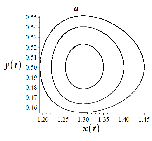
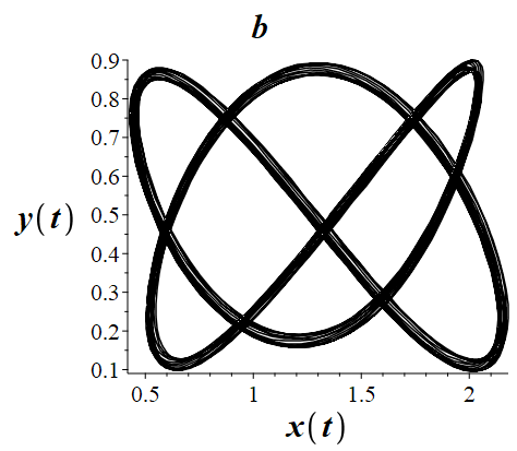
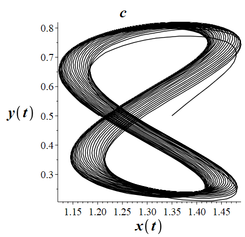
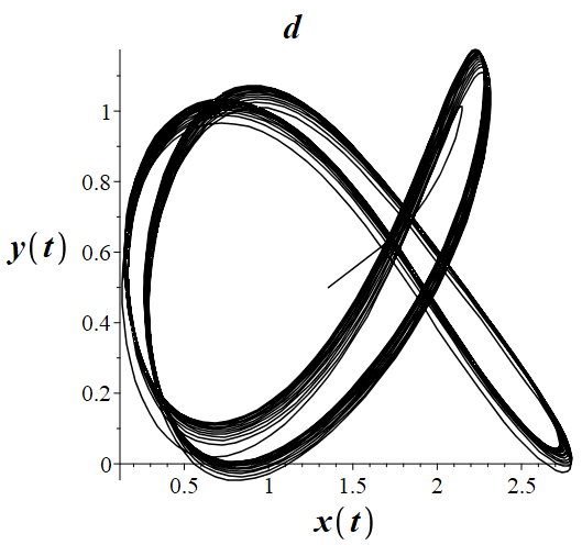
Figure 1: Regular modes

It can be seen that the phase trajectories in Figure 1a are in good agreement with the results of [4], which indicates the correctness of calculations using the ABM method. Figure 1b, c, d shows the phase trajectories obtained for various values of ${\alpha_{1}},{\alpha_{2}},{\delta_{1}},{\delta_{2}},{\omega_{1}},{\omega_{2}},\lambda$. We see that the phase trajectories are limit cycles, but of a more complex shape than in the classical case.

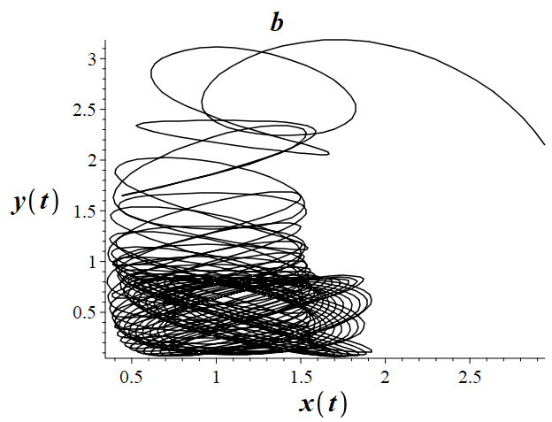
Figure 2: Chaotic modes

Figure 2 shows the phase trajectories that characterize chaotic regimes. Figure 2a is the origin of a chaotic attractor, Figure 2b is a chaotic attractor. Such modes need to be investigated in more detail, for example, by analogy with works [14, 15, 16]. Such a study will allow taking into account the necessary values of the model parameters for the existence of limit cycles.

VI Conclusion

In this paper, we have proposed a generalized Dubovsky model, taking into account the effects of heredity, as well as functions responsible for investment and management technologies. We examined the ABM method, investigated the accuracy of the method, and built phase trajectories. They showed that solutions can describe both regular regimes and chaotic regimes.

Of interest is the further study of the model in the following areas: the study of chaotic regimes, for example, using the spectra of the maximum Lyapunov exponents, the study of limit cycles, the determination of their lengths, for example, using the Poincaré sections, the economic interpretation of research results.

References

• Tarasov [2019] V. E. Tarasov, “On history of mathematical economics: Application of fractional calculus,” Mathematics 7, 06008 (2019), DOI:10.3390/math7060509.
• Alexander [2002] M. A. Alexander, The Kondratiev cycle: A generational interpretation (IUniverse, 2002).
• Makarov [2014] D. V. Makarov, “Economic and mathematical modeling innovation systems,” Vestnik KRAUNTs. Fiz.-mat. nauki 8, 66–70 (2014), DOI:10.18454/2079-6641-2014-8-1-66-70.
• Dubovsky [1995] S. V. Dubovsky, “The kondratiev cycle as an object of modelling,” Matem. Mod. 7, 65–74 (1995).
• Akayev [2008] A. A. Akayev, “Analysis of solutions of general equations of microeconomic dynamics,” Ekonomika i matematicheskie metody 44, 62–78 (2008).
• Makarov and Parovik [2016] D. I. Makarov and R. I. Parovik, “Modeling of the economic cycles using the theory of fractional calculus,” Journal of Internet Banking and Commerce 21 (2016).
• Parovik [2014] R. I. Parovik, “Numerical analysis some oscillation equations with fractional order derivatives,” Bulletin KRASEC. Physical and Mathematical Sciences 9, 34–38 (2014), DOI:10.18454/2313-0156-2014-9-2-34-38.
• Kilbas, Srivastava, and Trujillo [2006] A. A. Kilbas, H. M. Srivastava, and J. J. Trujillo, Theory and Applications of Fractional Differential Equations (Elsevier, 2006) p. 523.
• Oldham and Spanier [1974] K. B. Oldham and J. Spanier, The fractional calculus. Theory and applications of differentiation and integration to arbitrary order (Academic Press, 1974) p. 240.
• Miller and Ross [1993] K. S. Miller and B. Ross, An introduction to the fractional calculus and fractional differntial equations (A Wiley-Interscience publication, 1993) p. 384.
• Garrappa [2018] R. Garrappa, “Numerical solution of fractional differential equations: A survey and a software tutorial,” Mathematics 6 (2018), DOI:10.3390/math6020016.
• Yang and Liu [2006] C. Yang and F. Liu, “A computationally effective predictor-corrector method for simulating fractional-order dynamical control system,” ANZIAM J. 47, 168–184 (2006), DOI:10.21914/anziamj.v47i0.1037.
• Diethelm, Ford, and Freed [2002] K. Diethelm, N. J. Ford, and A. D. Freed, “A predictor-corrector approach for the numerical solution of fractional differential equations,” Nonlinear Dyn. 29, 3–22 (2002), DOI:10.1023/A:1016592219341.
• Parovik [2018] R. I. Parovik, “Research of the stability of some hereditary dynamic systems,” Journal of Physics: Conference Series 1141, 012079 (2018), DOI:10.1088/1742-6596/1141/1/012079.
• Cao [2020] Y. Cao, “Chaotic synchronization based on fractional order calculus financial system,” Chaos, Solitons & Fractals 130 (2020), DOI:10.1016/j.chaos.2019.109410.
• Diouf and Sene [2020] M. Diouf and N. Sene, “Analysis of the financial chaotic model with the fractional derivative operator,” Complexity 2020 (2020), DOI:10.1155/2020/9845031.