Model-Based Offline Planning with Trajectory Pruning

Abstract

The recent offline reinforcement learning (RL) studies have achieved much progress to make RL usable in real-world systems by learning policies from pre-collected datasets without environment interaction. Unfortunately, existing offline RL methods still face many practical challenges in real-world system control tasks, such as computational restriction during agent training and the requirement of extra control flexibility. The model-based planning framework provides an attractive alternative. However, most model-based planning algorithms are not designed for offline settings. Simply combining the ingredients of offline RL with existing methods either provides over-restrictive planning or leads to inferior performance. We propose a new light-weighted model-based offline planning framework, namely MOPP, which tackles the dilemma between the restrictions of offline learning and high-performance planning. MOPP encourages more aggressive trajectory rollout guided by the behavior policy learned from data, and prunes out problematic trajectories to avoid potential out-of-distribution samples. Experimental results show that MOPP provides competitive performance compared with existing model-based offline planning and RL approaches.

1 Introduction

Recent advances in offline reinforcement learning (RL) have taken an important step toward applying RL to real-world tasks. Although online RL algorithms have achieved great success in solving complex tasks such as games Silver et al. (2017) and robotic control Levine et al. (2016), they often require extensive interaction with the environment. This becomes a major obstacle for real-world applications, as collecting data with an unmatured policy via environment interaction can be expensive (e.g., robotics and healthcare) or dangerous (e.g., industrial control, autonomous driving). Fortunately, many real-world systems are designed to log or have sufficient pre-collected historical states and control sequences data. Offline RL tackles this challenge by training the agents offline using the logged dataset without interacting with the environment. The key insight of recent offline RL algorithms Fujimoto et al. (2019); Kumar et al. (2019); Wu et al. (2019); Yu et al. (2020) is to restrict policy learning stay “close” to the data distribution, which avoids the potential extrapolation error when evaluating on unknown out-of-distribution (OOD) samples.

However, implementing offline RL algorithms on real-world robotics and industrial control problems still faces some practical challenges. For example, many control agents have limited computational resources for policy learning, which require a light-weighted policy improvement procedure. Moreover, industrial control tasks often require extra control flexibility, such as occasionally changing reward signals due to altering system settings or certain devices, and involvement of state-based constraints due to safety considerations (e.g., restrict policy to avoid some unsafe states). Most existing offline RL algorithms need computationally extensive offline policy learning on a fixed task and do not offer any control flexibility.

Model-based planning framework provides an attractive solution to address the above challenges. The system dynamics can be learned offline based on the prior knowledge in the offline dataset. The policy optimization can be realized by leveraging model-predictive control (MPC) combined with a computationally efficient gradient-free trajectory optimizer such as the cross-entropy method (CEM) Botev et al. (2013) or model-predictive path integral (MPPI) control Williams et al. (2017). The planning process also allows easy integration with the change of reward signals or external state-based constraints during operation, without requiring re-training agents as needed in typical RL algorithms.

Most model-based planning methods are designed for online settings. Recent studies Wang and Ba (2020); Argenson and Dulac-Arnold (2021) have borrowed several ingredients of offline RL by learning a behavior cloning (BC) policy from the data to restrain trajectory rollouts during planning. This relieves OOD error during offline learning but unavoidably leads to over-restrictive planning. Limited by insufficient expressive power, behavior policies learned using BC often fit poorly on datasets generated by relatively random or multiple mixed data generating policies. Moreover, restricting trajectory rollouts by sampling near behavior policies also impacts the performance of trajectory optimizers (e.g., CEM, MPPI require reasonable state-action space coverage or diversity in order to find good actions), and hinders the full utilization of the generalizability of the dynamics model. Dynamic models may learn and generalize reasonably well in some low-density regions if the data pattern is simple and easy to learn. Strictly avoiding OOD samples may lead to over conservative planning which misses high reward actions.

We propose a new algorithmic framework, called Model-Based Offline Planning with Trajectory Prunning (MOPP), which allows sufficient yet safe trajectory rollouts and have superior performance compared with existing approaches. MOPP uses ensembles of expressive autoregressive dynamics models (ADM) Germain et al. (2015) to learn the behavior and dynamics from data to capture better prior knowledge about the system. To enforce better planning performance, MOPP encourages stronger exploration by allowing sampling from behavior policy with large deviation, as well as performing the greedy max-Q operation to select potentially high reward actions according to the Q-value function evaluated from the offline dataset. At the same time, to avoid undesirable OOD samples in trajectory rollouts, MOPP prunes out problematic trajectories with unknown state-action pairs detected by evaluating the uncertainty of the dynamics model. These strategies jointly result in an light-weighted and flexible algorithm that consistently outperforms the state-of-the-art model-based offline planning algorithm MBOP Argenson and Dulac-Arnold (2021), and also provides competitive performance as well as much better control flexibility compared with existing offline RL approaches.

2 Related Work

2.1 Offline reinforcement learning

Offline RL focuses on the setting that no interactive data collection is allowed during policy learning. The main difficulty of offline RL is the distributional shift Kumar et al. (2019), which occurs when the distribution induced by the learned policy deviates largely from the data distribution. Policies could make counterfactual queries on unknown OOD actions, causing overestimation of values that leads to non-rectifiable exploitation error during training.

Existing offline RL methods address this issue by following three main directions. Most model-free offline RL algorithms constrain the learned policy to stay close to a behavior policy through deviation clipping Fujimoto et al. (2019) or introducing additional divergence penalties (e.g., KL divergence, MMD or BC regularizer) Wu et al. (2019); Kumar et al. (2019); Fujimoto and Gu (2021); Xu et al. (2021). Other model-free offline RL algorithms instead learn a conservative, underestimated value function by modifying standard Bellman operator to avoid overly optimistic value estimates on OOD samples Kumar et al. (2020); Liu et al. (2020); Kostrikov et al. (2021); Buckman et al. (2020); Xu et al. (2022). Model-based offline RL methods Yu et al. (2020); Kidambi et al. (2020); Zhan et al. (2022), on the other hand, incorporate reward penalty based on the uncertainty of the dynamics model to handle the distributional shift issue. The underlying assumption is that the model will become increasingly inaccurate further from the behavior distribution, thus exhibits larger uncertainty. All these algorithms require a relatively intensive policy learning process as well as re-training for novel tasks, which make them less flexible for real-world control systems.

2.2 Model-based planning

The model-based planning framework provides a more flexible alternative for many real-world control scenarios. It does not need to learn an explicit policy, but instead, learns an approximated dynamics model of the environment and use a planning algorithm to find high return trajectories through this model. Online planning methods such as PETS Chua et al. (2018), POLO Lowrey et al. (2019), POPLIN Wang and Ba (2020), and PDDM Nagabandi et al. (2020) have shown good results using full state information in simulation and on real robotic tasks. These algorithms are generally built upon an MPC framework and use sample efficient random shooting algorithms such as CEM or MPPI for trajectory optimization. The recent MBOP Argenson and Dulac-Arnold (2021) further extends model-based planning to offline setting. MBOP is an extension of PDDM but learns a behavior policy as a prior for action sampling, and uses a value function to the extend planning horizon. The problem of MBOP is that its performance is strongly dependent on the learned behavior policy, which leads to over-restrictive planning and obstructs the full potential of the trajectory optimizer and the generalizability of the dynamics model. In this work, we propose MOPP to address the limitations of MBOP, which provides superior planning while avoids undesirable OOD samples in trajectory rollouts.

3 Preliminaries

We consider the Markov decision process (MDP) represented by a tuple as $(\mathcal{S},\mathcal{A},P,r,\gamma)$, where $\mathcal{S}$, $\mathcal{A}$ denote the state and action space, $P(s_{t+1}|s_{t},a_{t})$ the transition dynamics, $r(s_{t},a_{t})$ the reward function and $\gamma\in[0,1]$ the discounting factor. A policy $\pi(s)$ is a mapping from states to actions. We represent $R=\sum_{t=1}^{\infty}\gamma^{t}r(s_{t},a_{t})$ as the cumulative reward over an episode, which can be truncated to a specific horizon $H$ as $R_{H}$. Under offline setting, the algorithm only has access to a static dataset $\mathcal{B}$ generated by arbitrary unknown behavior policies $\pi_{b}$, and cannot interact further with the environment. One can use parameterized function approximators (e.g., neural networks) to learn the approximated environment dynamics $f_{m}(s_{t},a_{t})$ and behavior policy $f_{b}(s_{t})$ from the data. Our objective is to find an optimal policy $\pi^{*}(s_{t})=$ $\arg\max_{a\in\mathcal{A}}\sum_{t=1}^{H}\gamma^{t}r(s_{t},a_{t})$ given only dataset $\mathcal{B}$ that maximizes the finite-horizon cumulative reward with $\gamma=1$.

4 The MOPP Framework

MOPP is a model-based offline planning framework that tackles the fundamental dilemma between the restrictions of offline learning and high-performance planning. Planning by sampling strictly from behavior policy avoids potential OOD samples. The learned dynamics model can also be more accurate in high-density regions of the behavioral distribution. However, this also leads to over-restrictive planning, which forbids sufficient exploitation of the generalizability of the model as well as the information in the data. MOPP provides a novel solution to address this problem. It allows more aggressive sampling from behavior policy $f_{b}$ with boosted variance, and performs max-Q operation on sampled actions based on a Q-value function $Q_{b}$ evaluated based on behavioral data. This treatment can lead to potential OOD samples, so we simultaneously evaluate the uncertainty of the dynamics models to prune out problematic trajectory rollouts. To further enhance the performance, MOPP also uses highly expressive autoregressive dynamics model to learn the dynamics model $f_{m}$ and behavior policy $f_{b}$, as well as uses the value function to extend planning horizon and accelerate trajectory optimization.

4.1 Dynamics and Behavior Policy Learning

We use autoregressive dynamics model (ADM) Germain et al. (2015) to learn the probabilistic dynamics model $(r_{t},s_{t+1})=f_{m}(s_{t},a_{t})$ and behavior policy $a_{t}=f_{b}(s_{t})$. ADM is shown to have good performance in several offline RL problems due to its expressiveness and ability to capture non-unimodal dependencies in data Ghasemipour et al. (2021).

The ADM architecture used in our work is composed of several fully connected layers. Given the input $\boldsymbol{\mathrm{x}}$ (e.g., a state for $f_{b}$ or a state-action pair for $f_{m}$), an MLP first produces an embedding for the input, separate MLPs are then used to predict the mean and standard deviation of every dimension of the output. Let $o_{i}$ denote the $i$-th index of the predicted output $\boldsymbol{\mathrm{o}}$ and $\boldsymbol{\mathrm{o}}_{[<i]}$ represent a slice first up to and not including the $i$-th index following a given ordering. ADM decomposes the probability distribution of $\boldsymbol{\mathrm{o}}$ into a product of nested conditionals: $p(\boldsymbol{\mathrm{o}})=\prod_{i}^{I}p(o_{i}|\boldsymbol{\mathrm{x}},\boldsymbol{\mathrm{o}}_{[<i]})$. The parameters $\theta$ of the model $p(\boldsymbol{\mathrm{o}})$ can be learned by maximizing the log-likelihood on dataset $\mathcal{B}$: $L(\theta|\mathcal{B})=\sum_{\boldsymbol{\mathrm{x}}\in\mathcal{B}}\Big{[}\sum_{i=1}^{|\boldsymbol{\mathrm{o}}|}\log p(o_{i}|\boldsymbol{\mathrm{x}},\boldsymbol{\mathrm{o}}_{[<i]})\Big{]}$.

ADM assumes underlying conditional orderings of the data. Different orderings can potentially lead to different model behaviors. MOPP uses ensembles of $K$ ADMs with randomly permuted orderings for dynamics and behavior policy, which incorporates more diverse behaviors from each model to further enhance expressiveness.

4.2 Value Function Evaluation

Introducing a value function to extend the planning horizon in model-based planning algorithms have been shown to greatly accelerate and stabilize trajectory optimization in both online Lowrey et al. (2019) and offline Argenson and Dulac-Arnold (2021) settings. We follow this idea by learning a Q-value function $Q_{b}(s_{t},a_{t})$ using fitted Q evaluation (FQE) Le et al. (2019) with respect to actual behavior policy $\pi_{b}$ and $\gamma^{\prime}<1$:

A corresponding value function is further evaluated as $V_{b}(s_{t})=\mathbb{E}_{a\sim\pi_{b}}Q(s_{t},a)$. This provides a conservative estimate of values bond to behavioral distribution. MOPP adds $V_{b}$ to the cumulative returns of the trajectory rollouts to extend the planning horizon. This helps shorten horizon $H$ needed during planning. Besides, MOPP uses $Q_{b}$ to perform the max-Q operation and guide trajectory rollouts toward potentially high reward actions.

4.3 Offline Planning

MOPP is built upon the finite-horizon model predictive control (MPC) framework. It finds a locally optimal policy and a sequence of actions up to horizon $H$ based on the local knowledge of the dynamics model. At each step, the first action from the optimized sequence is executed. In MOPP, we solve a modified MPC problem which uses value estimate $V_{b}$ to extend the planning horizon:

$$\pi^{*}(s_{0})=\arg\max_{a_{0:H-1}}\mathbb{E}\Big{[}\sum_{t=0}^{H-1}\gamma^{t}r(s_{t},a_{t})+\gamma^{H}V_{b}(s_{H})\Big{]}$$ (2)

Obtaining the exact solution for the above problem can be rather costly, instead, we introduce a new guided trajectory rollout and pruning scheme, combined with an efficient gradient-free trajectory optimizer based on an extended version of MPPI Williams et al. (2017); Nagabandi et al. (2020).

Guided trajectory rollout. The key step in MOPP is to generate a set of proper action sequences to roll out trajectories that are used by the trajectory optimizer. Under offline settings, such trajectory rollouts can only be performed with the learned dynamics model $f_{m}$. Using randomly generated actions can lead to large exploitation errors during offline learning. MBOP uses a learned behavior policy as a prior to sample and roll out trajectories. This alleviates the OOD error but has several limitations. First, the learned behavior policy could have insufficient coverage on good actions in low-density regions or outside of the dataset distribution. This is common when the data are generated by low-performance behavior policies. Moreover, the dynamics model may generalize reasonably well in some low-density regions if the dynamics pattern is easy to learn. Strictly sampling from the behavior policy limits sufficient exploitation of the generalizability of the learned dynamics model. Finally, the lack of diversity in trajectories also hurts the performance of the trajectory optimizer.

MOPP also uses the behavior policy to guide trajectory rollouts, but with a higher degree of freedom. Let $\boldsymbol{\mu}^{a}(s_{t})=[\mu_{1}^{a}(s_{t}),\cdots,\mu_{|\mathcal{A}|}^{a}(s_{t})]^{T}$, $\boldsymbol{\sigma}^{a}(s_{t})=[\sigma_{1}^{a}(s_{t}),\cdots,\sigma_{|\mathcal{A}|}^{a}(s_{t})]^{T}$ denote the mean and standard deviation (std) of each dimension of the actions produced by the ADM behavior policy $f_{b}(s_{t})$. MOPP samples and selects an action at time step $t$ as:

where $\sigma_{M}>0$ is the std scaling parameter. We allow it to take larger values than $\max\boldsymbol{\sigma}^{a}$ to enable more aggressive sampling. In MBOP, the actions are sampled by adding a very small random noise on the outputs of a deterministic behavior policy, which assumes uniform variance across different action dimensions. By contrast, MOPP uses the means $\boldsymbol{\mu}^{a}$ and std $\boldsymbol{\sigma}^{a}$ boosted by $\sigma_{M}$ to sample actions ($\boldsymbol{\mu}^{a}$, $\boldsymbol{\sigma}^{a}$ from the ADM behavior policy $f_{b}$). This allows heterogeneous uncertainty levels across different action dimensions while preserves their relative relationship presented in data.

We further perform the max-Q operation on the sampled actions based on $Q_{b}$ to encourage potentially high reward actions. Note that $Q_{b}$ is evaluated entirely offline with respect to the behavior policy, which provides a conservative but relatively reliable long-term prior information. MOPP follows the treatment in PDDM and MBOP that mixes the obtained action $\hat{a}_{t}$ with the previous trajectory using a mixture coefficient $\beta$ to roll out trajectories with the dynamics model $f_{m}$. This produces a set of trajectory sequences $\boldsymbol{T}=\{T_{1},\dots,T_{N}\}$, with $T_{n}=\{(a_{t}^{n},s_{t}^{n})\}_{t=0}^{H-1},n\in\{1,\dots,N\}$.

Trajectory pruning. The previously generated trajectories in $\boldsymbol{T}$ may contain undesirable state-action pairs that are out-of-distribution or have large prediction errors using the dynamics model. Such samples need to be removed, but we also want to keep OOD samples at which the dynamics model can generalize well to extend the knowledge beyond the dataset $\mathcal{B}$. The uncertainty quantification method used in MOReL Kidambi et al. (2020) provides a nice fit for our purpose, which is evaluated as the prediction discrepancy of dynamics models $f_{m}^{l}$, $l\in 1,\dots,K$ in the ensemble: $\text{disc}(s,a)=\max_{i,j}\left\|f_{m}^{i}(s,a)-f_{m}^{j}(s,a)\right\|_{2}^{2}$.

Let $\boldsymbol{U}$ be the uncertainty matrix that holds the uncertainty measures $U_{n,t}=\text{disc}(s_{t}^{n},a_{t}^{n})$ for each step $t$ of trajectory $n$ in $\boldsymbol{T}$. MOPP filters the set of trajectories using the trajectory pruning procedure $TrajPrune(\boldsymbol{T},\boldsymbol{U})$. Denote $\boldsymbol{T}_{p}:=\{T_{n}|U_{n,t}<L,\forall t,n\}$, trajectory pruning returns a refined trajectory set for offline trajectory optimization as:

where $L$ is the uncertainty threshold, $N_{m}$ is the minimum number of trajectories used to run the trajectory optimizer (set as $N_{m}=0.2\lfloor N\rfloor$ in our implementation). The intuition of trajectory pruning is to remove undesirable state-action samples and produce a set of low uncertainty trajectories. MOPP first constructs a filtered trajectory set $\boldsymbol{T}_{p}$ that only contains trajectories with every state-action pair satisfying the uncertainty threshold. If $\boldsymbol{T}_{p}$ has less than $N_{m}$ trajectories, we sort the remaining trajectories in $\boldsymbol{T}-\boldsymbol{T}_{p}$ by the cumulative uncertainty (i.e. $\sum_{t}U_{n,t}$ with $T_{n}\in\boldsymbol{T}-\boldsymbol{T}_{p}$). The top $N_{m}-|\boldsymbol{T}_{p}|$ trajectories in the sorted set with the lowest overall uncertainty are added into $T_{p}$ as the final refined trajectory set.

Trajectory optimization. MOPP uses an extended version of the model predictive path integral (MPPI) Williams et al. (2017) trajectory optimizer that is used similarly in PDDM Nagabandi et al. (2020) and MBOP Argenson and Dulac-Arnold (2021). MOPP shoots out a set of trajectories $\boldsymbol{T}_{f}$ using the previous guided trajectory rollout and pruning procedure. Let $\boldsymbol{R}_{f}=\{R_{1},\dots,R_{|\boldsymbol{T}_{f}|}\}$ be the associated cumulative returns for trajectories in $\boldsymbol{T}_{f}$, the optimized action is obtained by re-weighting the actions of each trajectory according to their exponentiated returns:

$$A^{*}_{t}=\frac{\sum_{n=1}^{|\boldsymbol{T}_{f}|}\exp(\kappa R_{n})a_{t}^{n}}{\sum_{n=1}^{|\boldsymbol{T}_{f}|}\exp(\kappa R_{n})},\;\forall t=\{0,\dots,H-1\}$$ (5)

where $a_{t}^{n}$ is the action at step $t$ of trajectory $T_{n}\in\boldsymbol{T}_{f}$ and $\kappa$ is a re-weighting factor. The full algorithm is in Algorithm 1.

Algorithm 1 Complete algorithm of MOPP

0:  Offline dataset $\mathcal{B}$

1:  Train $Q_{b}$, $K_{1}$ dynamics models $f_{m}^{l}$ and $K_{2}$ behavior policies $f_{b}^{l}$ on $\mathcal{B}$. Initialize $A^{*}_{t}=0$, $\forall t\in\{0,\dots,H-1\}$.

2:  for $\tau=0...\infty$ do

3:     Observe $s_{\tau}$, initialize $\boldsymbol{T},\boldsymbol{R}=\emptyset$

4:     for $n=1,\dots,N$ do

5:        $s_{0}=s_{\tau}$, $R_{n}=0$, $T_{n}=\mathbf{null}$

6:        for $t=0\dots H-1$ do

7:           Sample action $\hat{a}_{t}$ using $f_{b}^{l}(s_{t})$ ($l$ randomly picked from $1\dots K_{2}$) according to Eq.(3)

8:           $\tilde{a}_{t}=(1-\beta)\hat{a}_{t}+{\beta}A^{*}_{t+1}$, ($A^{*}_{H}=A^{*}_{H-1}$)

9:           Append $(s_{t},\tilde{a}_{t})$ into trajectory $T_{n}$

10:           $s_{t+1}=f_{m}^{l^{\prime}}(s_{t},\tilde{a}_{t})^{s}$, $l^{\prime}$ randomly picked from $1\dots K_{1}$

11:           $R_{n}\leftarrow R_{n}+\frac{1}{K_{1}}\sum_{k=1}^{K_{1}}f_{m}^{k}(s_{t},\tilde{a}_{t})^{r}$

12:           $U_{n,t}=\max_{i,j}\left\|{f_{m}^{i}(s_{t},\tilde{a}_{t})-f_{m}^{j}(s_{t},\tilde{a}_{t})}\right\|_{2}^{2}$

13:        end for

14:        Compute $V_{b}(s_{H})=\sum_{i=1}^{K_{Q}}Q_{b}(s_{H},a_{i})/K_{Q}$, $\{a_{i}\}_{i=1}^{K_{Q}}$ are randomly sampled from $f_{b}^{l}(s_{H})$

15:        $R_{n}\leftarrow R_{n}+V_{b}(s_{H})$, $\boldsymbol{T}\leftarrow\boldsymbol{T}\cup\{T_{n}\}$, $\boldsymbol{R}\leftarrow\boldsymbol{R}\cup\{R_{n}\}$

16:     end for

17:     Compute $\boldsymbol{T}_{f}=TrajPrune(\boldsymbol{T},\boldsymbol{U})$ according to Eq.(4)

18:     Update $A^{*}_{t},\forall t=\{0,\dots,H-1\}$ using $\boldsymbol{T}_{f}$ and Eq.(5)

19:     Return optimized $a_{\tau}=A^{*}_{0}$

20:  end for

5 Experimental Results

		Model-based offline planning methods		Model-based offline RL methods
Dataset type	Environment	MBOP (MBOP $f_{b}^{\prime}$)	MOPP (ADM $f_{b}$)	MBPO	MOPO
random	halfcheetah	6.3$\pm$4.0 (0.0$\pm$0.0)	9.4$\pm$2.6 (2.2$\pm$2.2)	30.7$\pm$3.9	35.4$\pm$2.5
random	hopper	10.8$\pm$0.3 (9.0$\pm$0.2)	13.7$\pm$2.5 (9.8$\pm$0.7)	4.5$\pm$6.0	11.7$\pm$0.4
random	walker2d	8.1$\pm$5.5 (0.1$\pm$0.0)	6.3$\pm$0.1 (2.6$\pm$0.1)	8.6$\pm$8.1	13.6$\pm$2.6
medium	halfcheetah	44.6$\pm$0.8 (35.0$\pm$2.5)	44.7$\pm$2.6 (36.6$\pm$4.7)	28.3$\pm$22.7	42.3$\pm$1.6 4
medium	hopper	48.8$\pm$26.8 (48.1$\pm$26.2)	31.8$\pm$1.3 (30.0$\pm$0.8)	4.9$\pm$3.3	28.0$\pm$12.4
medium	walker2d	41.0$\pm$29.4 (15.4$\pm$24.7)	80.7$\pm$1.0 (15.6$\pm$22.5)	12.7$\pm$7.6	17.8$\pm$19.3
mixed	halfcheetah	42.3$\pm$0.9 (0.0$\pm$0.0)	43.1$\pm$4.3 (32.7$\pm$7.7)	47.3$\pm$12.6	53.1$\pm$2.0
mixed	hopper	12.4$\pm$5.8 (9.5$\pm$6.9)	32.3$\pm$5.9 (28.2$\pm$4.3)	49.8$\pm$30.4	67.5$\pm$24.7
mixed	walker2d	9.7$\pm$5.3 (11.5$\pm$7.3)	18.5$\pm$8.4 (12.9$\pm$5.7)	22.2$\pm$12.7	39.0$\pm$9.6
med-expert	halfcheetah	105.9$\pm$17.8 (90.8$\pm$26.9)	106.2$\pm$5.1 (37.6$\pm$6.5)	9.7$\pm$9.5	63.3$\pm$38.0
med-expert	hopper	55.1$\pm$44.3 (15$\pm$8.7)	95.4$\pm$28.0 (44.3$\pm$28.4)	56.0$\pm$34.5	23.7$\pm$6.0
med-expert	walker2d	70.2$\pm$36.2 (65.5$\pm$40.2)	92.9$\pm$14.1 (13.5$\pm$24.2)	7.6$\pm$3.7	44.6$\pm$12.9

Table 1: Results for D4RL MuJoCo tasks. The scores are normalized between 0 to 100 (0 and 100 correspond to a random policy and an expert SAC policy respectively). We report the mean scores and standard deviation (term after $\pm$) of each method. For MBOP and MOPP, we present the scores of the used behavior policies (MBOP $f_{b}^{\prime}$ and ADM $f_{b}$) in the parentheses.

We evaluate and compare the performance of MOPP with several state-of-the-art (SOTA) baselines on standard offline RL benchmark D4RL Fu et al. (2020). We conduct experiments on the widely-used MuJoCo tasks and the more complex Adroit hand manipulation tasks. All results are averaged based on 5 random seeds, with 20 episode runs per seed. In addition to performance comparison, we also conduct a comprehensive ablation study on each component in MOPP and evaluate its adaptability under varying objectives and constraints. Due to space limit, detailed experimental set-up, additional ablation on ADM behavior policy and dynamics model, as well as computational performance are included in the Appendix.

5.1 Comparative Evaluations

Performance on MoJoCo tasks. We evaluate the performance of MOPP on three tasks (halfcheetah, hopper and walker2d) and four dataset types (random, medium, mixed and med-expert) in the D4RL benchmark. We compare in Table 1 the performance of MOPP with several SOTA baselines, including model-based offline RL algorithms MBPO Janner et al. (2019) and MOPO Yu et al. (2020), as well as the SOTA model-based offline planning algorithm MBOP.

MOPP outperforms MBOP in most tasks, sometimes by a large margin. It is observed that MBOP is more dependent on its special behavior policy $a_{t}=f_{b}^{\prime}(s_{t},a_{t-1})$, which include previous step’s action as input. This will improve imitation performance under datasets generated by one or limited policies, as the next action may be correlated with the previous action, but could have negative impact on high-diversity or complex datasets (e.g., random and mixed). On the other hand, MOPP substantially outperforms its ADM behavior policy $f_{b}$ especially on the med-expert tasks, which shows great planning improvement upon a learned semi-performance policy.

Comparing with model-based offline RL methods MBPO and MOPO, we observe that MOPP performs better in medium and med-expert datasets, but less performant on higher-variance datasets such as random and mixed. Model-based offline RL methods can benefit from high-diversity datasets, in which they can learn better dynamics models and apply RL to find better policies. It should also be noted that training RL policies until convergence is costly and not adjustable after deployment. This will not be an issue for a light-weighted planning method like MOPP, as the planning process is executed in operation and suited well for controllers that require extra control flexibility. MOPP performs strongly in the med-expert dataset, which beats all other baselines and achieves close to or even higher scores compared with the expert SAC policy. This indicates that MOPP can effectively recover the performant data generating policies in the behavioral data and use planning to further enhance their performance.

Dataset	BC	BCQ	CQL	MOPO	MBOP	MOPP
pen-human	34.4	68.9	37.5	-0.6	53.4	73.5
hammer-human	1.5	0.5	4.4	0.3	14.8	2.8
door-human	0.5	0.0	9.9	-0.1	2.7	11.9
relocate-human	0.0	-0.1	0.2	-0.1	0.1	0.5
pen-cloned	56.9	44.0	39.2	4.6	63.2	73.2
hammer-cloned	0.8	0.4	2.1	0.4	4.2	4.9
door-cloned	-0.1	0.0	0.4	0.0	0.0	5.6
relocate-cloned	-0.1	-0.3	-0.1	-0.1	0.1	-0.1
pen-expert	85.1	114.9	107.0	3.7	105.5	149.5
hammer-expert	125.6	107.2	86.7	1.3	107.6	128.7
door-expert	34.9	99.0	101.5	0.0	101.2	105.3
relocate-expert	101.3	41.6	95.0	0.0	41.7	98.0

Table 2: Results for Adroit tasks. The scores are normalized between 0 to 100 (correspond to a random policy and an expert SAC policy).

Performance on Adroit tasks. We also evaluate the performance of MOPP in Table 2 on more complex Adroit high-dimensional robotic manipulation tasks with sparse reward, involving twirling a pen, hammering a nail, opening a door and picking/ moving a ball. The Adroit datasets are particularly hard, as the data are collected from a narrow expert data distributions (expert), human demonstrations (human), or a mixture of human demonstrations and imitation policies (cloned). Model-based offline RL methods are known to perform badly on such low-diversity datasets, as the dynamics models cannot be learned well (e.g., see results of MOPO). We compare MOPP with two more performant model-free offline RL algorithms, BCQ Fujimoto et al. (2019) and CQL Kumar et al. (2020). It is found that although MOPP is a model-based planning method, it performs surprisingly well in most of the cases. MOPP consistently outperforms the SOTA offline planning method MBOP, and in many tasks, it even outperforms the performant model-free offline RL baselines BCQ and CQL. The better performance of MOPP is a joint result of the inheritance of both an imitative behavior policy and more aggressive planning with the learned dynamics model.

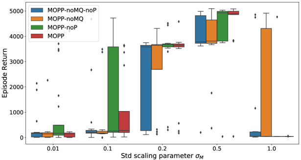
(a) Impacts of max-Q operation and trajectory pruning with different sampling aggressiveness ($\sigma_{M}$)

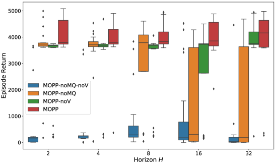
(b) Impacts of value function $V_{b}$ and max-Q operation with different planning horizon $H$

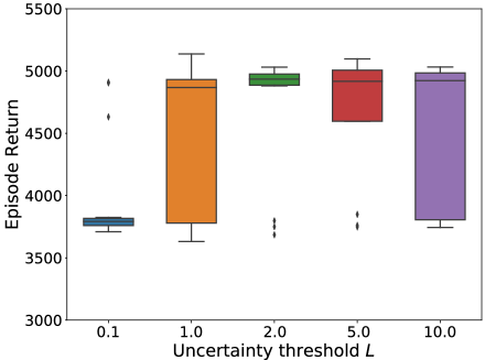
(c) Impact of uncertainty threshold $L$ ($\sigma_{M}=0.5$, $H=2$)

Figure 1: Ablation study on the walker2d-med-expert task. noMQ, noP, noV indicate MOPP without max-Q operation, trajectory pruning and value function $V_{b}$ respectively.

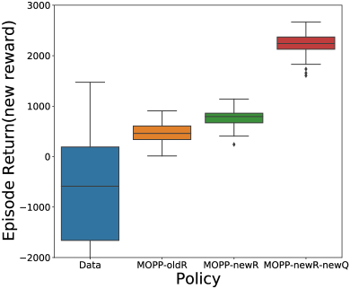
(a) Episode return under the new reward function

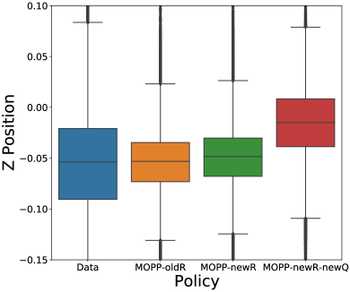
(b) The z-position of the optimized trajectories

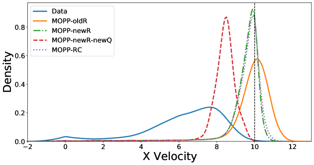
(c) Performance under x-velocity constraints.

Figure 2: Performance on halfcheetah-jump (a, b) and halfcheetah-constrained (c) tasks.

5.2 Ablation Study

We conduct ablation experiments on walker2d-med-expert task to understand the impact of key elements in MOPP. We first investigate in Figure 1(a) the level of sampling aggressiveness (controlled by std scaling parameter $\sigma_{M}$) on the performance of MOPP , as well as its relationship with the max-Q operation and trajectory pruning. It is observed that reasonably boosting the action sampling variance (e.g., increase $\sigma_{M}$ from $0.01$ to $0.5$) is beneficial. But overly aggressive exploration ($\sigma_{M}=1.0$) is detrimental, as it will introduce lots of undesired OOD samples during trajectory rollouts. When most trajectory rollouts are problematic, the trajectory pruning procedure is no longer effective, as there have to be at least $N_{m}$ trajectories in order to run the trajectory optimizer. When $\sigma_{M}$ is not too large, trajectory pruning is effective to control the planning variance and produces better performance, as is shown in the difference between MOPP-noP and MOPP under $\sigma_{M}=0.5$. Moreover, the max-Q operation in the guided trajectory rollout increases the sampling aggressiveness. When $\sigma_{M}$ is moderate, MOPP achieves a higher score than MOPP-noMQ. But when $\sigma_{M}=1.0$, the less aggressive MOPP-noMQ is the only variant of MOPP that is still possible to produce high episode returns. These suggest that carefully choosing the degree of sampling aggressiveness is important for MOPP to achieve the best performance.

We further examine the impacts of value function $V_{b}$ and max-Q operation on different planning horizons in Figure 1(b). It is observed that even with a very short horizon ($H=2$ and $4$), MOPP can attain good performance that is comparable to results using longer planning horizons. Moreover, MOPP achieves significantly higher scores compared with MOPP-noMQ-noV. We found that using max-Q operation on sampled actions provides stronger improvements, as MOPP-noMQ consistently perform worse than MOPP-noV. This might because that max-Q operation is performed at every step, while the value function is only added to the end of the cumulative return of a trajectory, thus providing stronger guidance on trajectory rollouts towards potentially high reward actions.

Finally, Figure 1(c) presents the impact of uncertainty threshold $L$ in trajectory pruning. We observe that both strictly avoid ($L=0.1$) or overly tolerant ($L=10.0$) unknown state-action pairs impact planning performance. Reasonably increase the tolerance of sample uncertainty ($L=2.0$) to allow sufficient exploration leads to the best result with low variance.

5.3 Evaluation on Control Flexibility

A major advantage of planning methods lies in their flexibility to incorporate varying objectives and extra constraints. These modifications can be easily incorporated in MOPP by revising the reward function or pruning out unqualified trajectory rollouts during operation. We construct two tasks to evaluated the control flexibility of MOPP:

• halfcheetah-jump: This task adds incentives on the z-position in the original reward function of halfcheetah, encouraging agent to run while jumping as high as possible.

• halfcheetah-constrained task adds a new constraint (x-velocity$\leq$10) to restrain agent from having very high x-velocity. Two ways are used to incorporate the constraint: 1) add reward penalty for x-velocity$>$10; 2) add penalties on the uncertainty measures $\boldsymbol{U}$ to allow trajectory pruning to filter out constraint violating trajectory rollouts.

Figure 2(a), (b) shows the performance of MOPP on the halfcheetah-jump task. By simply changing to the new reward function (MOPP-newR), MOPP is able to adapt and improve upon the average performance level in data and the original model (MOPP-oldR). The performance will be further improved by re-evaluating the Q-function (MOPP-newR-newQ). The offline evaluated value function $Q_{b}$ and the max-Q operation could have negative impact when the reward function is drastically different. In such cases, one only needs to re-evaluate a sub-component ($Q_{b}$ under the new reward) of MOPP to guarantee the best performance rather than re-train the whole model as in typical RL settings. Evaluating $Q_{b}$ via FQE is achieved by simple supervised learning, which is computationally very cheap compared with a costly RL procedure (see Appendix for discussion on computation performance).

Figure 2(c) presents the performance on the halfcheetah -constrained task. The original MOPP without constraint (MOPP-oldR) has lots of constraint violations (x-velocity$>$10). Incorporating a constraint penalty in reward (MOPP-newR) and pruning out constraint violating trajectories (MOPP-RC) achieve very similar performance. Both models effectively reduce constraint violations and have limited performance deterioration due to the extra constraint. Adding constraint penalty in the reward function while re-evaluating the $Q_{b}$ via FQE (MOPP-newR-newQ) leads to the safest policy.

6 Conclusion

We propose MOPP, a light-weighted model-based offline planning algorithm for real-world control tasks when online training is forbidden. MOPP is built upon an MPC framework that leverages behavior policies and dynamics models learned from an offline dataset to perform planning. MOPP avoids over-restrictive planning while enabling offline learning by encouraging more aggressive trajectory rollout guided by the learned behavior policy, and prunes out problematic trajectories by evaluating the uncertainty of dynamics models. Although MOPP is a planning method, benchmark experiments show that it provides competitive performance compared with the state-of-the-art offline RL and model-based planning methods.

Appendix

Appendix A Detailed Experiment Settings

A.1 Benchmark Datasets

We evaluate the performance of MOPP on the popular D4RL MuJoCo tasks (Halfcheetah, Hopper, Walker2d) and the more complex Adroit hand manipulation tasks (Pen, Hammer, Door, Relocate) Fu et al. [2020]. These tasks are visualized in Figure 4.

A.1.1 MoJoCo tasks

We test 12 problem settings in the D4RL MoJoCo benchmark, including three environments: halfcheetah, hopper, walker2d and four dataset types: random, medium, mixed and med-expert. The MoJoCo benchmark datasets are generated as follows:

• random: generated using a random policy to roll out 1M steps.

• medium: generated using a partially trained SAC policy Haarnoja et al. [2018] to roll out 1M steps.

• mixed: train an SAC policy until reaching a predefined threshold, and take the replay buffer as the dataset. This dataset is also termed medium-replay in the latest version of the D4RL paper.

• med-expert: generated by combining 1M samples from a expert policy and 1M samples from a partially trained policy.

A.1.2 Adroit tasks

The Adroit hand manipulation environment Rajeswaran et al. [2018] involves controlling a 24-DoF simulated Shadow Hand robot with twirling a pen (Pen), hammering a nail (Hammer), opening a door (Door) and picking up and moving a ball (Relocate). Adroit tasks are substantially more challenging than the MoJoCo tasks, as the dataset is collected from human demonstrations and fine-tuned online RL expert policies with narrow data distributions on sparse reward, high-dimensional control tasks. The Adroit tasks have three dataset types:

• human: contains a small amount of demonstration data from a human, 25 trajectories per task.

• expert: contains a larger amount of expert data from a fine-tuned online RL policy.

• cloned: generated by training an imitation policy on the demonstrations, running the policy, and mixing data at a 50-50 ratio with demonstrations.

A.2 Hyperparameters Used in the D4RL Benchmark Experiments

In Table 3, we present the hyperparameters used for runs of MOPP on the D4RL benchmark. We kept most hyperparameter settings close to MBOP Argenson and Dulac-Arnold [2021] to make our results comparable to those reported in the MBOP paper. In the ablation study, all the hyperparameters of MOPP are the same as that in Table 3 except the varied parameters in the ablation experiments. The hyperparameter $L$ is selected based on the 85th percentile value of the uncertainty measures computed from the offline dataset. In addition to the hyperparameters reported in the table, for all experiments, we use $N_{m}=0.2\lfloor N\rfloor$, $K_{1}=K_{2}=3$ and $K_{Q}=10$ (see Algorithm 1 in the main article for details).

MoJoCo HalfCheetah
Dataset	$H$	$\kappa$	$\beta$	$L$	$\sigma_{M}$	$N$
random	4	3	0	4	1.15	100
medium	2	3	0	5	0.45	100
mixed	4	3	0	5	0.5	100
med-expert	2	1	0	7	0.55	100
MoJoCo Hopper
Dataset	$H$	$\kappa$	$\beta$	$L$	$\sigma_{M}$	$N$
random	4	10	0	0.5	0.65	100
medium	4	0.3	0	1	0.25	100
mixed	4	0.3	0	1	0.6	100
med-expert	10	3	0	1	0.4	100
MoJoCo Walker2d
Dataset	$H$	$\kappa$	$\beta$	$L$	$\sigma_{M}$	$N$
random	8	0.3	0	8	0.05	1000
medium	2	0.1	0	7	0.55	1000
mixed	8	3	0	8	0.2	1000
med-expert	2	1	0	7	0.4	1000
Adroit Pen
Dataset	$H$	$\kappa$	$\beta$	$L$	$\sigma_{M}$	$N$
human	4	0.3	0	0.1	0.8	100
cloned	4	0.3	0	1.7	0.8	100
expert	4	0.03	0	4.4	0.8	100
Adroit Hammer
Dataset	$H$	$\kappa$	$\beta$	$L$	$\sigma_{M}$	$N$
human	4	0.3	0	0.3	1.0	100
cloned	4	0.3	0	0.5	0.8	100
expert	4	0.3	0	1.4	0.7	100
Adroit Door
Dataset	$H$	$\kappa$	$\beta$	$L$	$\sigma_{M}$	$N$
human	4	0.3	0	1.2	0.8	100
cloned	4	0.3	0	0.3	0.8	100
expert	4	0.03	0	0.1	0.7	100
Adroit Relocate
Dataset	$H$	$\kappa$	$\beta$	$L$	$\sigma_{M}$	$N$
human	4	0.3	0	1.0	0.8	100
cloned	4	0.3	0	0.4	0.8	100
expert	16	0.3	0	0.1	0.4	100

Table 3: Hyperparameters of MOPP used in the D4RL benchmark experiments

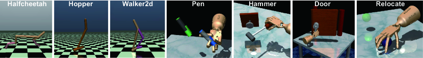
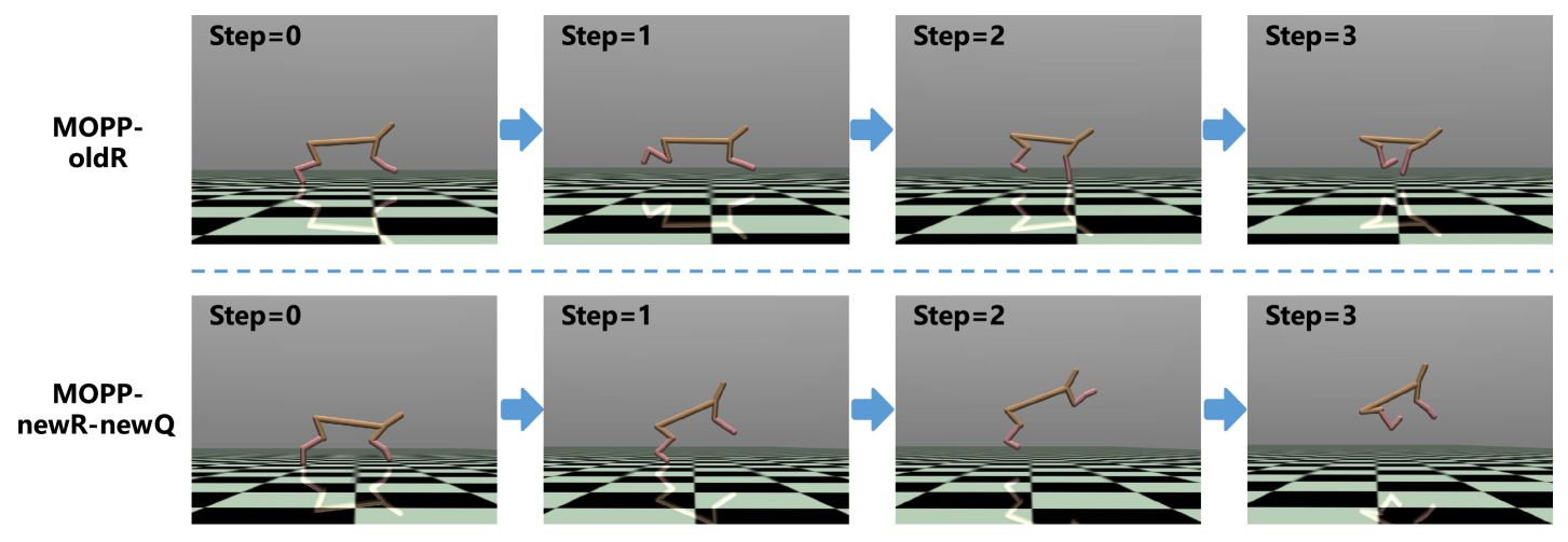
Figure 3: Visualization of the evaluated tasks

Figure 4: Illustrations of the original halfcheetah and the halfcheetah-jump tasks. The top row shows the results of MOPP with the original objective (MOPP-oldR). The bottom row shows the results obtained using MOPP with the new reward function and re-evaluated Q-function (MOPP-newR-newQ). It is observed that the halfcheetah agent using MOPP-newR-newQ adapts to the new objective that is running while jumping as high as possible.

A.3 Flexibility of Incorporating Varying Objectives and Constraints

We modify the original halfcheetah task and construct two new tasks (halfcheetah-jump and halfcheetah -constrained) to evaluate the flexibility and generalizibility of MOPP on new tasks with varying objectives and extra constraints. In both tasks, MOPP is trained using the entire 1M steps training replay buffer of SAC on the original halfcheetah task. We modify the reward function or introduce rollout constraints in MOPP during planning. To test for best performance and examine the impact of max-Q operation, we also report the results of MOPP with re-evaluated Q-functions under the new reward function via FQE. The results of MOPP and its variants of the new tasks are reported in Figure 2 in the main article. All results are computed based on 6 random seeds, with 20 episode runs per seed.

A.3.1 Control under varying objective

In the halfcheetah -jump task, we modify the objective of the original halfcheetah agent, which encourages the agent to have higher z-position, leading to a run and jump behavior. The modified reward function in the new objective is:

$$r^{\prime}=\alpha_{r}\cdot r+(1-\alpha_{r})\cdot 100\cdot z$$ (6)

where $r$ is the original reward of the halfcheetah task, and $z$ denotes the z-position of the halfcheetah agent. In our experiment, $\alpha_{r}$ is set as 0.4. Note that our halfcheetah-jump task is different from the one reported in the MOPO paper Yu et al. [2020] which sets the maximum velocity to be 3 in both behavior policy and its revised reward to only encourage the jump behavior.

A.3.2 Constrained control

In the halfcheetah- constrained task, we introduce a state-based constraint to the original halfcheetah task. We constrain the velocity along the x-axis ($v_{x}$) of the halfcheetah agent below a certain threshold (10 m/s). Two implementations are tested in our experiments:

• Reward penalization: Adding a reward penalty for $v_{x}>10$ in the reward function:

  $$r^{\prime}=\alpha_{c}\cdot r+(1-\alpha_{c})\cdot 100\cdot\min(10-v_{x},0)$$ (7)

  where $r$ is the original reward of the halfcheetah task and the weight $\alpha_{c}$ is set as 0.5 in the experiments.

• Rollout constraint: We filter out the trajectories that violate the state-based constraint during trajectory pruning in MOPP. This is achieved as a rollout constraint by adding penalties to the uncertainty measures $U_{n,t}$ of the constraint violating trajectory rollouts.

  $$U_{n,t}^{\prime}=U_{n,t}+100\cdot\max(v_{x}-10,0)$$ (8)

  Note that due to the existence of the minimum number of required trajectories $N_{m}$ to run the trajectory optimizer, it is possible that some unsafe trajectories will remain after trajectory pruning if most of the trajectory rollouts violate the constraint. The advantage of rollout constraint is that it does not alter the reward function, thus has no impact on the Q-function learned from the behavioral data.

Dataset type	Environment	MBOP (MBOP $f_{b}^{\prime}$)	MOPP-ADM $f_{m}$ (BC)	MOPP-ADM $f_{m}$ (ADM $f_{b}$)	MOPP-FC $f_{m}$ (BC)	MOPP-FC $f_{m}$ (ADM $f_{b}$)
random	halfcheetah	6.3$\pm$4.0 (0.0$\pm$0.0)	9.1$\pm$0.2 (2.2$\pm$2.2)	9.4$\pm$2.6 (2.2$\pm$2.2)	7.9 $\pm$ 0.3 (2.2$\pm$2.2)	7.9$\pm$0.3 (2.2$\pm$2.2)
random	hopper	10.8$\pm$0.3 (9.0$\pm$0.2)	11.9$\pm$0.1 (10.0$\pm$0.7)	13.7$\pm$2.5 (9.8$\pm$0.7)	11.8$\pm$0.2 (10.0$\pm$0.7)	12.1$\pm$0.2 (9.8$\pm$0.7)
random	walker2d	8.1$\pm$5.5 (0.1$\pm$0.0)	4.9$\pm$0.9 (6.2$\pm$2.2)	6.3$\pm$0.1 (2.6$\pm$0.1)	6.7$\pm$0.2 (6.2$\pm$2.2)	6.5$\pm$0.1 (2.6$\pm$0.1)
medium	halfcheetah	44.6$\pm$0.8 (35.0$\pm$2.5)	44.5$\pm$0.3 (36.7$\pm$4.1)	44.7$\pm$2.6 (36.6$\pm$4.7)	45.0$\pm$0.4(36.7$\pm$4.1)	45.1$\pm$0.3 (36.6$\pm$4.7)
medium	hopper	48.8$\pm$26.8 (48.1$\pm$26.2)	28.2$\pm$8.8 (30.4$\pm$0.9)	31.8$\pm$1.3 (30.0$\pm$0.8)	28.0$\pm$9.1 (30.4$\pm$0.9)	27.3$\pm$9.9 (30.0$\pm$0.8)
medium	walker2d	41.0$\pm$29.4 (15.4$\pm$24.7)	82.3$\pm$0.9 (15.0$\pm$19.8)	80.7$\pm$1.0 (15.6$\pm$22.5)	81.3$\pm$4.2 (15.0$\pm$19.8)	81.4$\pm$1.3 (15.6$\pm$22.5)
mixed	halfcheetah	42.3$\pm$0.9 (0.0$\pm$0.0)	41.4$\pm$1.9 (31.8$\pm$7.2)	43.1$\pm$4.3 (32.7$\pm$7.7)	40.8$\pm$0.8 (31.8$\pm$7.2)	40.3$\pm$0.7 (32.7$\pm$7.7)
mixed	hopper	12.4$\pm$5.8 (9.5$\pm$6.9)	30.6$\pm$2.7 (20.0$\pm$7.7)	32.3$\pm$5.9 (28.2$\pm$4.3)	30.5$\pm$2.9 (20.0$\pm$7.7)	28.0$\pm$0.9 (28.2$\pm$4.3)
mixed	walker2d	9.7$\pm$5.3 (11.5$\pm$7.3)	16.5$\pm$7.4 (12.9$\pm$4.5)	18.5$\pm$8.4 (12.9$\pm$5.7)	15.4$\pm$7.4 (12.9$\pm$4.5)	15.0$\pm$6.7 (12.9$\pm$5.7)
med-expert	halfcheetah	105.9$\pm$17.8 (90.8$\pm$26.9)	103.7$\pm$11.0 (37.6$\pm$6.5)	106.2$\pm$5.1 (37.6$\pm$6.5)	96.7$\pm$10.1 (37.6$\pm$6.5)	86.9$\pm$22.1 (37.6$\pm$6.5)
med-expert	hopper	55.1$\pm$44.3 (15$\pm$8.7)	94.4$\pm$31.6 (34.1$\pm$18.7)	95.4$\pm$28.0 (44.3$\pm$28.4)	103.9$\pm$23.8 (34.1$\pm$18.7)	51.6$\pm$36.0 (44.3$\pm$28.4)
med-expert	walker2d	70.2$\pm$36.2 (65.5$\pm$40.2)	88.3$\pm$38.8 (6.6$\pm$13.8)	92.9$\pm$14.1 (13.5$\pm$24.2)	87.9$\pm$38.8 (6.6$\pm$13.8)	85.6$\pm$10.6 (13.5$\pm$24.2)

Table 4: Ablation results on D4RL MuJoCo tasks for MOPP on using feed-forward (FC $f_{m}$) and ADM (ADM $f_{m}$) dynamics model as well as BC and ADM behavior policy $f_{b}$. The feed-forward dynamics model (FC $f_{m}$) is the same as that reported in MBOP Argenson and Dulac-Arnold [2021]. The scores are normalized between 0 to 100 (0 and 100 correspond to a random policy and an expert SAC policy respectively). The scores of the used behavior policies (MBOP $f_{b}^{\prime}$, BC and ADM $f_{b}$) in the parentheses. All results are computed based on 5 random seeds, with 20 episode runs per seed.

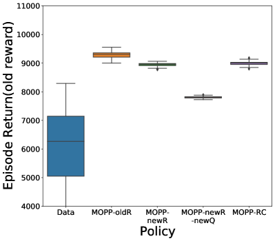
(a) Episode return under the original reward function

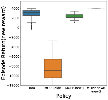
(b) Episode return under the new reward function

Figure 5: Additional results of MOPP on halfcheetah- constrained task

Figure 5 presents additional results on the episode returns of MOPP and its variants under the original and new reward function of the halfcheetah-constrained task. Adding additional constraints to ensure safety will sacrifice the episode return measured by the original reward function. We observe that MOPP-newR and MOPP-RC can effective reduce constraint violations and have limited performance deterioration under the existence of extra constraint. Adding the constraint penalty in reward function and re-evaluating the Q-function (MOPP-newR-newQ) achieves safest policy but have substantially drop in episode return measured by the old reward function, but it still has improved episode return as measured by the new reward function.

Appendix B Ablation on the ADM Dynamics Model and Behavior Policy

We also report in Table 4 the additional ablation results on the impacts of using feed-forward neural networks or ADM for dynamics model and behavior policy in MOPP. For the dynamics model in MOPP, we compare the same feed-forward network structure as used in MBOP Argenson and Dulac-Arnold [2021] (FC $f_{m}$) as well as our ADM dynamics model (ADM $f_{m}$). For the behavior policy, we report the results of the behavior policy used in MBOP (MBOP $f_{b}^{\prime}$), the standard BC policy and the ADM behavior policy $f_{b}$ used in MOPP.

As expected, the more expressive ADM dynamics model and behavior policies are found to have positive impact on the performance. Regarding the behavior policy, MBOP uses a special behavior policy that include the action of previous step as input $a_{t}=f_{b}^{\prime}(s_{t},a_{t-1})$, thus not directly comparable. This design will improve imitation performance under datasets generated by one or limited data generating policies, as the next action may be correlated with the previous action, but could have negative impact on high-diversity (e.g., random and mixed) or complex datasets. The more expressive ADM behavior policy $f_{b}$ outperforms BC policy in most tasks, except for the random dataset. As the expressiveness of a probabilistic model provides little help when fitting random actions. Under the same ADM dynamics model (ADM $f_{m}$), MOPP with ADM behavior policy $f_{b}$ consistently outperform the variant with BC policy. However, using ADM $f_{b}$ with feed-forward dynamics model (FC $f_{m}$) does not provide improved performance, perhaps due to less reliable trajectory rollout with the feed-forward dynamics model. Using the more expressive ADM dynamics model is observed to have larger impact on MOPP’s performance as compared to the different choice of behavior policy. MOPP with ADM $f_{m}$ achieves improved performance in the majority of tasks under both ADM $f_{b}$ and BC policy. Moreover, MOPP with ADM $f_{m}$ and $f_{b}$ achieves the best overall performance.

Appendix C Execution Speed

The execution speeds (control steps/second) of MOPP on the D4RL Walker2d and Hopper tasks are reported in Table 5. The tests are conducted on an Intel Xeon 2.2GHz CPU computer (no GPU involved) with simulator time included. It is observed that MOPP can easily achieve multiple controls within 1 second, which is useable for many robotics and industrial control tasks. Using longer planning horizons will increase the computation time. But we also observe in Table 5 that with a moderate planning horizon (e.g., $H=8$), MOPP is already able to achieve high episode returns by incorporating the value function $V_{b}$ and max-Q operation with $Q_{b}$. The execution speed of MOPP can be further speed up by reducing the number of trajectory rollouts $N$ or use a shorter planning horizon.

In the cases when the reward function is drastically changed during system operation, to guarantee the best model performance, it is suggested to re-evaluate the Q-value function based on the new reward function. In MOPP, the Q-value function is evaluated via FQE, which is performed by simple supervised learning and computationally cheap to train. Table 6 presents the computation time for Q-value evaluation under different size of behavioral data for HalfCheetah and Hopper tasks. The entire computation can be finished in a relatively short time with limited resources.

	Walker2d		Hopper
H	Freq.	Ep. return	Freq.	Ep. return
4	2.69	3885.2 $\pm$ 941.8	4.22	2539.6 $\pm$ 1051.7
8	2.13	4032.8 $\pm$ 450.8	3.25	2847.9 $\pm$ 992.6
16	1.50	4000.2 $\pm$ 643.8	2.41	2974.9 $\pm$ 1037.9

Table 5: Execution speeds (control frequency (Hz)) and episode returns of MOPP. Models are trained on med-expert dataset.

	HalfCheetah		Hopper
Data size	1,000,000	200,000	1,000,000	200,000
Time cost(min)	26.0	5.2	24.7	4.9

Table 6: Computation time of the Q-value function evaluation via FQE. Batch size: 512, epochs: 40. Tests are conducted on a quad-core CPU and 8 GB memory computer (no GPU involved).

Appendix D Model Configurations of MOPP

For all the D4RL MuJoCo and Adroit benchmark tasks, we use the following model configurations for MOPP.

D.1 ADM behavior policy and dynamics model

The ADM behavior policy $f_{b}$ and dynamics model $f_{m}$ share the same model configurations, which are set as follows:

• Embedding layer: (500,)

• FC layers for separate dimension of output: (200, 100)

• Number of networks in the ensemble: 3

• Learning rate: 0.001

• Training steps: 5e+5

• Optimizer: Adam

D.2 Q-value network $Q_{b}$

The model configurations of $Q_{b}$ are set as follows:

• FC layers: (500, 500)

• Learning rate: 0.001

• Training steps: 5e+5

• Optimizer: Adam

References

- Argenson and Dulac-Arnold [2021] Arthur Argenson and Gabriel Dulac-Arnold. Model-based offline planning. In International Conference on Learning Representations, 2021.
- Botev et al. [2013] Zdravko I Botev, Dirk P Kroese, Reuven Y Rubinstein, and Pierre L’Ecuyer. The cross-entropy method for optimization. In Handbook of statistics, volume 31, pages 35–59. Elsevier, 2013.
- Buckman et al. [2020] Jacob Buckman, Carles Gelada, and Marc G Bellemare. The importance of pessimism in fixed-dataset policy optimization. In International Conference on Learning Representations, 2020.
- Chua et al. [2018] Kurtland Chua, Roberto Calandra, Rowan McAllister, and Sergey Levine. Deep reinforcement learning in a handful of trials using probabilistic dynamics models. In Advances in Neural Information Processing Systems, pages 4754–4765, 2018.
- Fu et al. [2020] Justin Fu, Aviral Kumar, Ofir Nachum, George Tucker, and Sergey Levine. D4rl: Datasets for deep data-driven reinforcement learning. arXiv preprint arXiv:2004.07219, 2020.
- Fujimoto and Gu [2021] Scott Fujimoto and Shixiang Shane Gu. A minimalist approach to offline reinforcement learning. In Advances in Neural Information Processing Systems, 2021.
- Fujimoto et al. [2019] Scott Fujimoto, David Meger, and Doina Precup. Off-policy deep reinforcement learning without exploration. In International Conference on Machine Learning, pages 2052–2062. PMLR, 2019.
- Germain et al. [2015] Mathieu Germain, Karol Gregor, Iain Murray, and Hugo Larochelle. Made: Masked autoencoder for distribution estimation. In International Conference on Machine Learning, pages 881–889, 2015.
- Ghasemipour et al. [2021] Seyed Kamyar Seyed Ghasemipour, Dale Schuurmans, and Shixiang Shane Gu. Emaq: Expected-max q-learning operator for simple yet effective offline and online rl. In International Conference on Machine Learning, pages 3682–3691. PMLR, 2021.
- Haarnoja et al. [2018] Tuomas Haarnoja, Aurick Zhou, Pieter Abbeel, and Sergey Levine. Soft actor-critic: Off-policy maximum entropy deep reinforcement learning with a stochastic actor. In International Conference on Machine Learning, pages 1861–1870. PMLR, 2018.
- Janner et al. [2019] Michael Janner, Justin Fu, Marvin Zhang, and Sergey Levine. When to trust your model: Model-based policy optimization. In Advances in Neural Information Processing Systems, pages 12519–12530, 2019.
- Kidambi et al. [2020] Rahul Kidambi, Aravind Rajeswaran, Praneeth Netrapalli, and Thorsten Joachims. Morel: Model-based offline reinforcement learning. In Advances in Neural Information Processing Systems, pages 21810–21823, 2020.
- Kostrikov et al. [2021] Ilya Kostrikov, Rob Fergus, Jonathan Tompson, and Ofir Nachum. Offline reinforcement learning with fisher divergence critic regularization. In International Conference on Machine Learning, 2021.
- Kumar et al. [2019] Aviral Kumar, Justin Fu, Matthew Soh, George Tucker, and Sergey Levine. Stabilizing off-policy q-learning via bootstrapping error reduction. In Advances in Neural Information Processing Systems, pages 11761–11771, 2019.
- Kumar et al. [2020] Aviral Kumar, Aurick Zhou, George Tucker, and Sergey Levine. Conservative q-learning for offline reinforcement learning. In Advances in Neural Information Processing Systems, pages 1179–1191, 2020.
- Le et al. [2019] Hoang M Le, Cameron Voloshin, and Yisong Yue. Batch policy learning under constraints. In International Conference on Machine Learning, pages 3703–3712. PMLR, 2019.
- Levine et al. [2016] Sergey Levine, Chelsea Finn, Trevor Darrell, and Pieter Abbeel. End-to-end training of deep visuomotor policies. The Journal of Machine Learning Research, 17(1):1334–1373, 2016.
- Liu et al. [2020] Yao Liu, Adith Swaminathan, Alekh Agarwal, and Emma Brunskill. Provably good batch off-policy reinforcement learning without great exploration. In Advances in Neural Information Processing Systems, pages 1264–1274, 2020.
- Lowrey et al. [2019] Kendall Lowrey, Aravind Rajeswaran, Sham Kakade, Emanuel Todorov, and Igor Mordatch. Plan online, learn offline: Efficient learning and exploration via model-based control. In International Conference on Learning Representations, 2019.
- Nagabandi et al. [2020] Anusha Nagabandi, Kurt Konolige, Sergey Levine, and Vikash Kumar. Deep dynamics models for learning dexterous manipulation. In Conference on Robot Learning, pages 1101–1112. PMLR, 2020.
- Rajeswaran et al. [2018] Aravind Rajeswaran, Vikash Kumar, Abhishek Gupta, Giulia Vezzani, John Schulman, Emanuel Todorov, and Sergey Levine. Learning complex dexterous manipulation with deep reinforcement learning and demonstrations. In Proceedings of Robotics: Science and Systems, June 2018.
- Silver et al. [2017] David Silver, Julian Schrittwieser, Karen Simonyan, Ioannis Antonoglou, Aja Huang, Arthur Guez, Thomas Hubert, Lucas Baker, Matthew Lai, Adrian Bolton, et al. Mastering the game of go without human knowledge. nature, 550(7676):354–359, 2017.
- Wang and Ba [2020] Tingwu Wang and Jimmy Ba. Exploring model-based planning with policy networks. In International Conference on Learning Representations, 2020.
- Williams et al. [2017] Grady Williams, Andrew Aldrich, and Evangelos A Theodorou. Model predictive path integral control: From theory to parallel computation. Journal of Guidance, Control, and Dynamics, 40(2):344–357, 2017.
- Wu et al. [2019] Yifan Wu, George Tucker, and Ofir Nachum. Behavior regularized offline reinforcement learning. arXiv preprint arXiv:1911.11361, 2019.
- Xu et al. [2021] Haoran Xu, Xianyuan Zhan, Jianxiong Li, and Honglei Yin. Offline reinforcement learning with soft behavior regularization. arXiv preprint arXiv:2110.07395, 2021.
- Xu et al. [2022] Haoran Xu, Xianyuan Zhan, and Xiangyu Zhu. Constraints penalized q-learning for safe offline reinforcement learning. In Proceedings of the AAAI Conference on Artificial Intelligence, 2022.
- Yu et al. [2020] Tianhe Yu, Garrett Thomas, Lantao Yu, Stefano Ermon, James Zou, Sergey Levine, Chelsea Finn, and Tengyu Ma. Mopo: Model-based offline policy optimization. In Advances in Neural Information Processing Systems, pages 14129–14142, 2020.
- Zhan et al. [2022] Xianyuan Zhan, Haoran Xu, Yue Zhang, Yusen Huo, Xiangyu Zhu, Honglei Yin, and Yu Zheng. Deepthermal: Combustion optimization for thermal power generating units using offline reinforcement learning. In Proceedings of the AAAI Conference on Artificial Intelligence, 2022.