Regret Analysis of Distributed Online LQR Control
for Unknown LTI Systems

Abstract

Online optimization has recently opened avenues to study optimal control for time-varying cost functions that are unknown in advance. Inspired by this line of research, we study the distributed online linear quadratic regulator (LQR) problem for linear time-invariant (LTI) systems with unknown dynamics. Consider a multi-agent network where each agent is modeled as a LTI system. The network has a global time-varying quadratic cost, which may evolve adversarially and is only partially observed by each agent sequentially. The goal of the network is to collectively (i) estimate the unknown dynamics and (ii) compute local control sequences competitive to the best centralized policy in hindsight, which minimizes the sum of network costs over time. This problem is formulated as a regret minimization. We propose a distributed variant of the online LQR algorithm, where agents compute their system estimates during an exploration stage. Each agent then applies distributed online gradient descent on a semi-definite programming (SDP) whose feasible set is based on the agent system estimate. We prove that with high probability the regret bound of our proposed algorithm scales as $O(T^{2/3}\log T)$, implying the consensus of all agents over time. We also provide simulation results verifying our theoretical guarantee.

I Introduction

In recent years, there has been a significant interest on problems arising at the interface of control and machine learning. Among classical control problems, LQR control [1, 2, 3] is a prominent point in case. LQR control centers around LTI systems, where the control-state pairs introduce a quadratic cost with time-invariant parameters. When the dynamics of the LTI system is known, for finite-horizon and infinite-horizon problems, the optimal controllers have closed-form solutions, which can be derived by solving the corresponding Riccati equations.

Despite the excellent insights on the LQR problem provided by the classical control theory, in practical problems we might encounter two challenges. (I) The environment could change in an unpredictable way, which makes the cost parameters time-varying and unknown in advance (e.g., in variable-supply electricity production and building climate control with time-varying energy costs [4]). (II) Furthermore, the dynamics of the LTI system may be unknown. The former challenge has motivated research at the interface of online optimization and control, where online LQR problem is cast as a regret minimization and the performance of an online algorithm is compared to that of the best fixed control policy in hindsight. The regret metric is particularly meaningful in the online setting, where the cost parameters are unknown in advance. The focus of online LQR is on the finite-time performance from a learning-theory perspective (see details of this literature in item 4 of Subsection I-A). The latter challenge is addressed via adaptive control in general. In this case, the learner must strike a balance between exploration (estimating the system dynamics while preventing the cumulative cost from going unbounded) and exploitation (using the estimates to compete with the performance of the optimal controller) [5, 6, 7, 8].

In this work, we consider the distributed online LQR problem for a network of LTI systems with unknown dynamics. Each system is represented by an agent in the network that has a global time-varying quadratic cost. The cost sequence may evolve adversarially and is only partially observed by each agent sequentially. The goal of each agent is to generate a control sequence that is competitive to that of the best centralized policy in hindsight, formulated by regret. This setting can be applied for modeling the energy consumption in mobile sensor networks as described in Example 1. To address the problem, we propose a decentralized algorithm with two phases. In the exploration phase, each agent computes system estimates using the EXTRA algorithm [9], which is an iterative decentralized optimization method. In the exploitation phase, agents perform distributed online gradient descent on a SDP (whose feasible set is constructed by local system estimates) and extract the control policies accordingly. We prove that if every agent maintains a good balance between system identification (exploration) and online control (exploitation), the regret is bounded by $O(T^{2/3}\log T)$, where $T$ is the total number of iterations. This implies that the agents reach consensus and collectively compete with the best fixed controller in hindsight. Besides the exploration-exploitation trade-off, the main technical challenge is that the decentralized system identification step results in different SDPs across agents. This implies that the feasible set of SDP varies from one agent to another, and we cannot directly use distributed online optimization results on a common feasible set. We draw upon techniques from alternating projections to tackle this problem. Our technical proof is provided in the Appendix (Section VI). We also provide simulation results verifying our regret bound.

I-A Related Literature

(1) Distributed LQR Control: Distributed LQR has been widely studied in the control literature. A number of works focus on multi-agent systems with known, identical decoupled dynamics. In [10], a distributed control design is proposed by solving a single LQR problem whose size scales with the maximum degree of the graph capturing the network. The authors of [11] derive the necessary condition for an optimal distributed controller design, resulting in a non-convex optimization problem. The work of [12] addresses a multi-agent network, where the dynamics of each agent is a single integrator. The authors of [12] show that the computation of the optimal controller requires the knowledge of the graph and the initial information of all agents. Given the difficulty of precisely solving the optimal distributed controller, Jiao et al. [13] provide the sufficient conditions to obtain sub-optimal controllers. All of the aforementioned works need global information such as network topology to compute the controllers. On the other hand, Jiao et al. [14] propose a decentralized method to compute the controllers and show that the system will reach consensus. For the case of unknown dynamics, Alemzadeh et al. [15] propose a distributed Q-learning algorithm for dynamically decoupled systems. There are other works focusing on distributed control without assuming identical decoupled sub-systems. Fattahi et al. [16] study distributed controllers for unknown and sparse LTI systems. Furieri et al. [17] address model-free methods for distributed LQR problems and provide sample-complexity bounds for problems with local gradient dominance property (e.g., quadratically-invariant problems). The work of [18] investigates the convergence of distributed controllers to a global minimum for quadratically invariant problems with first-order methods.

(2) System Identification of LTI Systems: For solving LQR problems with unknown dynamics, we first need to learn the underlying system. To provide performance guarantee for the controller, it is important to explicitly quantify the uncertainty of the model estimate. The classical theory of system identification for LTI systems (e.g., [19, 20, 21, 22]) characterizes the asymptotic properties of the estimators. On the contrary, recent results in statistical learning focus on finite-time guarantees. In [23], it is shown that for fully observable systems, a least-squares estimator can learn the underlying dynamics from multiple trajectories. These results are later extended to the estimation using a single trajectory [24, 25]. For partially observable systems, estimators with polynomial sample complexities are provided in the literature (e.g., [26, 27, 28, 29]), and the work of [30] improves the sample complexity to be poly-logarithmic.

(3) Online LQR with Unknown Dynamics and Time-Invariant Costs: There is a recent line of research dealing with LQR control problems with unknown dynamics. Several techniques are proposed using (i) gradient estimation (e.g., [31, 32, 33, 34]), (ii) the estimation of dynamics matrices and derivation of the controller by considering the estimation uncertainty (e.g., [7, 23, 8, 35, 36, 37]), and (iii) wave-filtering [38, 39].

(4) Online Control with Time-Varying Costs: Recently, there has been a significant interest in studying linear dynamical systems with time-varying cost functions, where online learning techniques are applied. This literature investigates two scenarios: I) Known Systems: Cohen et al. [4] study the SDP relaxation for online LQR control and establish a regret bound of $O(\sqrt{T})$ for known LTI systems with time-varying quadratic costs. Agarwal et al. [40] propose the disturbance-action policy parameterization and reduce the online control problem to online convex optimization with memory. They show that for adversarial disturbances and arbitrary time-varying convex functions, the regret is $O(\sqrt{T})$. Agarwal et al. [41] consider the case of time-varying strongly-convex functions and improve the regret bound to $O(\text{poly}(\text{log}T))$. Simchowitz et al. [42] further extend the $O(\text{poly}(\text{log}T))$ regret bound to partially observable systems with semi-adversarial disturbances. Yu et al. [43] incorporate the idea of model predictive control into online LQR control with time-invariant cost function and correct noise predictions. Zhang et al. [44] extend this idea to the setup where costs are time-varying and accurate disturbance predictions are not accessible. Both of them provide the dynamic regret bound with a term shrinking exponentially with the prediction window. Our previous work [45] studies the distributed online LQR control with known dynamics and provides the regret bound of $O(\sqrt{T})$. II) Unknown Systems: For fully observable systems, Hazan et al. [46] derive the regret of $O(T^{2/3})$ for time-varying convex functions with adversarial noises. For partially observable systems, the work of [42] addresses the cases of (i) convex functions with adversarial noises and (ii) strongly-convex functions with semi-adversarial noises, and provide regret bounds of $O(T^{2/3})$ and $O(\sqrt{T})$, respectively. Lale et al. [47] establish an $O(\text{poly}(\text{log}T))$ regret bound for the case of stochastic perturbations, time-varying strongly-convex functions, and partially observed states.

Our work lies precisely at the interface of distributed LQR, online LQR and adaptive control, addressing distributed online LQR with unknown dynamics.

II Preliminaries and Problem Formulation

II-A Notation

$[n]$	The set $\{1,2,\ldots,n\}$ for any integer $n$
$\text{Tr}(\cdot)$	The trace operator
$\lVert\cdot\rVert$	Euclidean (spectral) norm of a vector (matrix)
$\lVert\cdot\rVert_{F}$	Frobenius norm of a matrix
$\mathrm{E}[\cdot]$	The expectation operator
$\Pi_{\mathcal{S}}[\cdot]$	The operator for the projection to set $\mathcal{S}$
$[\mathbf{A}]_{ij}$	The entry in the $i$-th row and $j$-th column of $\mathbf{A}$
$[\mathbf{A}]_{:,j}$	The $j$-th column of $\mathbf{A}$
$\mathbf{A}\bullet\mathbf{B}$	$\text{Tr}(\mathbf{A}^{\top}\mathbf{B})$
$\mathbf{A}\succeq\mathbf{B}$	$(\mathbf{A}-\mathbf{B})$ is positive semi-definite
$\mathbb{1}$	The vector of all ones
$\mathbf{e}_{i}$	The $i$-th basis vector
$\text{vec}(\mathbf{A})$	Vectorized version of the matrix $\mathbf{A}$

II-B Distributed Online LQR Control with Unknown Dynamics

We consider a multi-agent network of $m$ LTI systems, where the dynamics of agent $i$ is given as,

$$\mathbf{x}_{i,t+1}=\mathbf{A}\mathbf{x}_{i,t}+\mathbf{B}\mathbf{u}_{i,t}+\mathbf{w}_{i,t},\quad i\in[m]$$

and $\mathbf{x}_{i,t}\in\mathrm{R}^{d}$ and $\mathbf{u}_{i,t}\in\mathrm{R}^{k}$ represent agent $i$ state and control (or action) at time $t$, respectively. Furthermore, $\mathbf{A}\in\mathrm{R}^{d\times d}$, $\mathbf{B}\in\mathrm{R}^{d\times k}$, and $\mathbf{w}_{i,t}$ is a Gaussian noise with zero mean and covariance $\mathbf{W}\succeq\sigma^{2}\mathbf{I}$. The system parameters $(\mathbf{A},\mathbf{B})$ are unknown to all agents and need to be estimated. The noise sequence $\{\mathbf{w}_{i,t}\}$ is independent over time and agents. We also assume that $\lVert[\mathbf{A}\>\mathbf{B}]\rVert_{F}\leq\vartheta$ and let $n:=d+k$ for the presentation simplicity.

Departing from the classical LQR control, we consider the online distributed LQR problem, where the cost functions are unknown in advance. At round $t$, agent $i$ receives the state $\mathbf{x}_{i,t}$ and applies the action $\mathbf{u}_{i,t}$. Then, positive semi-definite cost matrices $\mathbf{Q}_{i,t}$ and $\mathbf{R}_{i,t}$ are revealed, and the agent incurs the cost $\mathbf{x}_{i,t}^{\top}\mathbf{Q}_{i,t}\mathbf{x}_{i,t}+\mathbf{u}_{i,t}^{\top}\mathbf{R}_{i,t}\mathbf{u}_{i,t}$. Throughout this paper, we assume that $\text{Tr}(\mathbf{Q}_{i,t}),\text{Tr}(\mathbf{R}_{i,t})\leq C$ for all $i,t$ and some $C>0$. Agent $i$ follows a policy that selects the control $\mathbf{u}_{i,t}$ based on the observed cost matrices $\mathbf{Q}_{i,1},\ldots,\mathbf{Q}_{i,t-1}$ and $\mathbf{R}_{i,1},\ldots,\mathbf{R}_{i,t-1}$, as well as the information received from its local neighborhood. This policy is not driven based on individual costs. On the contrary, agents follow a team goal through minimizing a cost collectively as we describe next.

Centralized Benchmark: In order to gauge the performance of a distributed online LQR algorithm, we require a centralized benchmark. In this paper, we focus on the finite-horizon problem, where for a centralized policy $\pi$, the cost after $T$ steps is given as

$$J_{T}(\pi)=\mathrm{E}\left[\sum_{t=1}^{T}{\mathbf{x}_{t}^{\pi}}^{\top}\mathbf{Q}_{t}\mathbf{x}_{t}^{\pi}+{\mathbf{u}_{t}^{\pi}}^{\top}\mathbf{R}_{t}\mathbf{u}_{t}^{\pi}\right],$$ (1)

where $\mathbf{Q}_{t}=\sum_{i=1}^{m}\mathbf{Q}_{i,t}$ and $\mathbf{R}_{t}=\sum_{i=1}^{m}\mathbf{R}_{i,t}$, and the expectation is over the possible randomness of the policy as well as the noise. The superscript $\pi$ in $\mathbf{u}_{t}^{\pi}$ and $\mathbf{x}_{t}^{\pi}$ alludes that the state-control pairs are chosen by the policy $\pi$, given full access to cost matrices of all agents. Notice that in the infinite-horizon version of the problem with time-invariant cost matrices $(\mathbf{Q},\mathbf{R})$, where the goal is to minimize $\lim_{T\rightarrow\infty}J_{T}(\pi)/T$, it is well-known that for a controllable LTI system $(\mathbf{A},\mathbf{B})$, the optimal policy is given by the constant linear feedback, i.e., $\mathbf{u}_{t}^{\pi}=\mathbf{K}\mathbf{x}_{t}^{\pi}$ for a matrix $\mathbf{K}\in\mathrm{R}^{k\times d}$.

Regret Definition: The goal of a distributed online LQR algorithm $\mathcal{A}$ is to mimic the performance of an ideal centralized algorithm that solves (1). The main two challenges are (i) the online nature of the problem, where cost matrices become available sequentially, and (ii) the distributed setup, where agent $i$ only receives information about the sequence $\{\mathbf{Q}_{i,t},\mathbf{R}_{i,t}\}$ while the cost is based on $\{\mathbf{Q}_{t},\mathbf{R}_{t}\}$. In this setting, each agent $j$ locally generates the control sequence $\{\mathbf{u}_{j,t}\}_{t=1}^{T}$, that is competitive to the best policy among a benchmark policy class $\Pi$. This can be formulated as minimizing the individual regret, which is defined as follows

$$\text{Regret}_{T}^{j}(\mathcal{A}):=J_{T}^{j}(\mathcal{A})-\min_{\pi\in\Pi}J_{T}(\pi),$$ (2)

for agent $j\in[m]$, where

$$J_{T}^{j}(\mathcal{A}) =\mathrm{E}\left[\sum_{t=1}^{T}{\mathbf{x}_{j,t}^{\mathcal{A}}}^{\top}\mathbf{Q}_{t}\mathbf{x}_{j,t}^{\mathcal{A}}+{\mathbf{u}_{j,t}^{\mathcal{A}}}^{\top}\mathbf{R}_{t}\mathbf{u}_{j,t}^{\mathcal{A}}\right].$$ (3)

A successful distributed algorithm is one that keeps the regret sublinear with respect to $T$. Of course, this also depends on the choice of the benchmark policy class $\Pi$, which is assumed to be the set of strongly stable policies (to be defined precisely in Section II-C). Since the underlying dynamics is unknown, agents have to find a good trade-off between exploration (estimating the system parameters) and exploitation (keeping the regret sublinear).

Network Structure: The underlying network topology is represented by a symmetric doubly stochastic matrix $\mathbf{P}$, i.e., all elements of $\mathbf{P}$ are non-negative and $\sum_{i=1}^{m}[\mathbf{P}]_{ji}=\sum_{j=1}^{m}[\mathbf{P}]_{ji}=1$. If $[\mathbf{P}]_{ji}>0$, agents $i$ and $j$ are neighbors; otherwise $[\mathbf{P}]_{ji}=0$. The network is assumed to be connected, i.e., for any two agents $i,j\in[m]$, there is a (potentially multi-hop) path from $i$ to $j$. We also assume $\mathbf{P}$ has a positive diagonal. Then, there exists a geometric mixing bound for $\mathbf{P}$ [48], such that $\sum_{j=1}^{m}\left|[\mathbf{P}^{k}]_{ji}-1/m\right|\leq\sqrt{m}\beta^{k},\>i\in[m],$ where $\beta$ is the second largest singular value of $\mathbf{P}$. Agents cannot share their observed cost functions with each other, but they can exchange a local parameter used for constructing the controllers. The communication is consistent with the structure of $\mathbf{P}$. We elaborate on this in the algorithm description.

Example 1.

Our framework can be used for minimizing the energy consumption in mobile sensor networks (MSNs) [49] in time-varying settings. Consider a MSN where at time $t$ the total mobility cost (or budget) of sensors is modeled by matrices $(\mathbf{Q}_{t},\mathbf{R}_{t})$. Each agent $i$ has a local budget of $(\mathbf{Q}_{i,t},\mathbf{R}_{i,t})$, but the team goal is to design actions that minimize the global network cost over time. Then, actions of this MSN should be guided to minimize the global cost in (1), though each sensor only has local information.

II-C Strong Stability and Sequential Strong Stability

We consider the set of strongly stable linear (i.e., $\mathbf{u}=\mathbf{K}\mathbf{x}$) controllers as the benchmark policy class. Following [4], we define the notion of strong stability as follows.

Definition 1.

(Strong Stability) A linear policy $\mathbf{K}$ is $(\kappa,\gamma)$-strongly stable (for $\kappa>0$ and $0<\gamma\leq 1$) for the LTI system $(\mathbf{A},\mathbf{B})$, if $\lVert\mathbf{K}\rVert\leq\kappa$, and there exist matrices $\mathbf{L}$ and $\mathbf{H}$ such that $\mathbf{A}+\mathbf{B}\mathbf{K}=\mathbf{H}\mathbf{L}\mathbf{H}^{-1}$, with $\lVert\mathbf{L}\rVert\leq 1-\gamma$ and $\lVert\mathbf{H}\rVert\|\mathbf{H}^{-1}\|\leq\kappa$.

Strong stability is a quantitative version of stability, in the sense that any stable policy is strongly stable for some $\kappa$ and $\gamma$, and vice versa [4]. A strongly stable policy ensures fast mixing and exponential convergence to a steady-state distribution. In particular, for the LTI system $\mathbf{x}_{t+1}=\mathbf{A}\mathbf{x}_{t}+\mathbf{B}\mathbf{u}_{t}+\mathbf{w}_{t}$, if a $(\kappa,\gamma)$-strongly stable policy $\mathbf{K}$ is applied ($\mathbf{u}_{t}=\mathbf{K}\mathbf{x}_{t}$), $\widehat{\mathbf{X}}_{t}$ (the state covariance matrix of $\mathbf{x}_{t}$) converges to $\mathbf{X}$ (the steady-state covariance matrix) with the following exponential rate

$$\lVert\widehat{\mathbf{X}}_{t}-\mathbf{X}\rVert\leq\kappa^{2}e^{-2\gamma t}\lVert\widehat{\mathbf{X}}_{0}-\mathbf{X}\rVert.$$

See Lemma 3.2 in [4] for details. The sequential nature of online LQR control requires another notion of strong stability, called sequential strong stability [4], defined as follows.

Definition 2.

(Sequential Strong Stability) A sequence of linear policies $\{\mathbf{K}_{t}\}_{t=1}^{T}$ is $(\kappa,\gamma)$-strongly stable if there exist matrices $\{\mathbf{H}_{t}\}_{t=1}^{T}$ and $\{\mathbf{L}_{t}\}_{t=1}^{T}$ such that $\mathbf{A}+\mathbf{B}\mathbf{K}_{t}=\mathbf{H}_{t}\mathbf{L}_{t}\mathbf{H}_{t}^{-1}$ for all $t$ with the following properties,

1. $\lVert\mathbf{L}_{t}\rVert\leq 1-\gamma$ and $\lVert\mathbf{K}_{t}\rVert\leq\kappa$.

2. $\lVert\mathbf{H}_{t}\rVert\leq\beta^{\prime}$ and $\lVert\mathbf{H}_{t}^{-1}\rVert\leq 1/\alpha^{\prime}$ with $\kappa=\beta^{\prime}/\alpha^{\prime}$.

3. $\lVert\mathbf{H}_{t+1}^{-1}\mathbf{H}_{t}\rVert\leq 1+\gamma/2$.

Sequential strong stability generalizes strong stability to the time-varying scenario, where a sequence of policies $\{\mathbf{K}_{t}\}_{t=1}^{T}$ is used. The convergence of steady-state covariance matrices induced by $\{\mathbf{K}_{t}\}_{t=1}^{T}$ is characterized as follows.

Lemma 1.

(Lemma 3.5 in [4]) Suppose a time-varying policy ($\mathbf{u}_{t}=\mathbf{K}_{t}\mathbf{x}_{t}$) is applied. Denote the steady-state covariance matrix of $\mathbf{K}_{t}$ as $\mathbf{X}_{t}$. If $\{\mathbf{K}_{t}\}$ are $(\kappa,\gamma)$-sequentially strongly stable and $\lVert\mathbf{X}_{t}-\mathbf{X}_{t-1}\rVert\leq\eta$, $\widehat{\mathbf{X}}_{t}$ (the state covariance matrix of $\mathbf{x}_{t}$) converges to $\mathbf{X}_{t}$ as follows

$$\lVert\widehat{\mathbf{X}}_{t+1}-\mathbf{X}_{t+1}\rVert\leq\kappa^{2}e^{-\gamma t}\lVert\widehat{\mathbf{X}}_{1}-\mathbf{X}_{1}\rVert+\frac{2\eta\kappa^{2}}{\gamma}.$$

II-D SDP Relaxation for LQR Control

For the following dynamical system

$$\mathbf{x}_{t+1}=\mathbf{A}\mathbf{x}_{t}+\mathbf{B}\mathbf{u}_{t}+\mathbf{w}_{t},\quad\mathbf{w}_{t}\sim\mathcal{N}(0,\mathbf{W}),$$

the infinite-horizon version of (1), i.e., $\text{minimize}\lim_{T\rightarrow\infty}J_{T}(\pi)/T,$ with fixed cost matrices $\mathbf{Q}$ and $\mathbf{R}$ can be relaxed via a SDP when the steady-state distribution exists. For $\nu>0$, the SDP relaxation is formulated as [4]

$$\begin{split}\text{minimize}\quad&J(\Sigma)=\begin{pmatrix}\mathbf{Q}&0\\ 0&\mathbf{R}\end{pmatrix}\bullet\Sigma\\ \text{subject to}\quad&\Sigma_{\mathbf{x}\mathbf{x}}=[\mathbf{A}\>\mathbf{B}]\Sigma[\mathbf{A}\>\mathbf{B}]^{\top}+\mathbf{W},\\ &\Sigma\succeq 0,\quad\text{Tr}(\Sigma)\leq\nu,\end{split}$$ (4)

where

$$\Sigma=\begin{pmatrix}\Sigma_{\mathbf{x}\mathbf{x}}&\Sigma_{\mathbf{x}\mathbf{u}}\\ \Sigma_{\mathbf{u}\mathbf{x}}&\Sigma_{\mathbf{u}\mathbf{u}}\end{pmatrix}.$$

Recall that in the online LQR problem, we deal with time-varying cost matrices $(\mathbf{Q}_{t},\mathbf{R}_{t})$, and for any $t\in[T]$, the above SDP yields different solutions. In fact, for any feasible solution $\Sigma$ of the above SDP, a strongly stable controller $\mathbf{K}=\Sigma_{\mathbf{x}\mathbf{u}}^{\top}\Sigma_{\mathbf{x}\mathbf{x}}^{-1}$ can be extracted. The steady-state covariance matrix induced by this controller is also feasible for the SDP and its cost is at most that of $\Sigma$ (see Theorem 4.2 in [4]). Moreover, for any (slowly-varying) sequence of feasible solutions to the SDP, the induced controller sequence is sequentially strongly-stable.

II-E Challenges of Distributed Online LQR for Unknown Dynamical Systems

The works of [4] and [45] tackle the centralized and decentralized online LQR, respectively. To keep the regret sublinear, the key idea in online LQR is to construct sequentially strongly stable controllers using online gradient descent (projected to the feasible set of SDP in (4)). However, in our work, given that system parameters $(\mathbf{A},\mathbf{B})$ are unknown, the agents must perform a system identification first. The system identification step results in two challenges: (i) an exploration-exploitation trade-off to keep the regret sublinear, and (ii) different SDPs across agents as a result of decentralized estimation. The latter is particularly challenging, because as we can see in (4), each agent only has a local estimate of $(\mathbf{A},\mathbf{B})$, so the SDPs will have different feasible sets across agents, and we cannot directly apply distributed online optimization results on a common feasible set (e.g., [50, 51]). In this work, we propose an algorithm (in the next section) for which we prove that an extracted controller based on a precise enough system estimates $(\widehat{\mathbf{A}},\widehat{\mathbf{B}})$ is strongly stable w.r.t. the system $(\mathbf{A},\mathbf{B})$.

III Algorithm and Theoretical Results

We now develop the distributed online LQR algorithm for unknown systems and study its theoretical regret bound.

III-A Algorithm

Our proposed method is outlined in Algorithm 1. In the first $T_{0}+1$ iterations, we need to collect data for the system identification. Suppose that each agent has access to a controller $\mathbf{K}_{0}$, which is $(\kappa_{0},\gamma_{0})$-strongly stable w.r.t. the system $(\mathbf{A},\mathbf{B})$. This controller can be different across agents, but for the presentation simplicity, we assume that agents use the same controller $\mathbf{K}_{0}$. The knowledge of such controller is a common assumption in centralized LQR (see e.g., [7, 8]). In this period, agent $i$ at time $t$ applies the control $\mathbf{u}_{i,t}\sim\mathcal{N}(\mathbf{K}_{0}\mathbf{x}_{i,t},2\sigma^{2}\kappa^{2}_{0}\cdot\mathbf{I})$, which prevents the state $\mathbf{x}_{i,t}$ from going unbounded (lines 2-7). For the next $T_{1}$ iterations, all agents perform the system identification step by solving a distributed least-squares (LS) problem. In this step, the global LS problem is formed using the data collected by all agents, where each agent local cost is only based on its own collected data. Here, we can use any iterative distributed optimization algorithm to get precise enough system estimates. We employ the EXTRA algorithm [9] since it achieves a geometric rate for strongly convex problems, and it can be implemented in a decentralized fashion (lines 8-16). After $T_{0}+T_{1}+1$ iterations, each agent $i$ at time $t$ runs a distributed online gradient descent on the SDP (4), where the local cost is defined w.r.t. matrices $\mathbf{Q}_{i,t}$ and $\mathbf{R}_{i,t}$, and the feasible set is defined w.r.t. system estimates $(\widehat{\mathbf{A}}_{i,t},\widehat{\mathbf{B}}_{i,t})$. A control matrix $\mathbf{K}_{i,t}$ is then extracted from the update of $\Sigma_{i,t}$ and is used to determine the action. In particular, $\mathbf{u}_{i,t}$ is sampled from a Gaussian distribution $\mathcal{N}(\mathbf{K}_{i,t}\mathbf{x}_{i,t},\mathbf{V}_{i,t})$, which entails $\mathrm{E}[\mathbf{u}_{i,t}|\mathcal{F}_{t}]=\mathbf{K}_{i,t}\mathbf{x}_{i,t}$, where $\mathcal{F}_{t}$ is the smallest $\sigma$-field containing the information about all agents up to time $t$ (lines 17-26). The choice of $\mathbf{V}_{i,t}$ is due to a technical reason. It ensures the fast convergence of the covariance matrix of $\mathbf{x}_{i,t}$ to the steady-state covariance matrix, when applying $\mathbf{K}_{i,t}$ to the underlying system $(\mathbf{A},\mathbf{B})$.

III-B Theoretical Result: Regret Bound

In this section, we present our main theoretical result. By applying Algorithm 1, we show that for a multi-agent network of unknown LTI systems (with a connected communication graph), the individual regret of an arbitrary agent is upper-bounded by $O(T^{2/3}\log T)$, which implies that the agents collectively perform as well as the best fixed controller in hindsight for large enough $T$.

Algorithm 1 Online Distributed LQR Control with Unknown Dynamics

1:  Require: number of agents $m$, doubly stochastic matrix $\mathbf{P}\in\mathrm{R}^{m\times m}$, parameter $\nu$, step size $\eta$, a $(\kappa_{0},\gamma_{0})$-strongly stable controller $\mathbf{K}_{0}$ w.r.t. system matrices $(\mathbf{A},\mathbf{B})$, covariance parameter of the noise $\sigma$, parameter $\vartheta$. Initialize: $\mathbf{x}_{i,1}=0,\forall i\in[m]$.

2:  for $t=1,2,\ldots,T_{0}+1$ do

3:     for $i=1,2,\ldots,m$ do

4:        Receive $\mathbf{x}_{i,t}$

5:        Perform action $\mathbf{u}_{i,t}\sim\mathcal{N}(\mathbf{K}_{0}\mathbf{x}_{i,t},2\sigma^{2}\kappa^{2}_{0}\cdot\mathbf{I})$

6:     end for

7:  end for

8:  After the first $(T_{0}+1)$ iterations, each agent $i$ uses the collected data to form the local function

$$f_{i}(\mathbf{A},\mathbf{B}):=\sum_{t=1}^{T_{0}}\lVert[\mathbf{A}\>\mathbf{B}]\mathbf{z}_{i,t}-\mathbf{x}_{i,t+1}\rVert^{2}+\frac{\sigma^{2}\vartheta^{-2}}{m}\lVert[\mathbf{A}\>\mathbf{B}]\rVert_{F}^{2},$$

where $\mathbf{z}_{i,t}=[\mathbf{x}_{i,t}^{\top}\>\mathbf{u}_{i,t}^{\top}]^{\top}$.

9:  Choose the step size $\alpha$ following the result in [9] and denote $\tilde{\mathbf{P}}:=\frac{\mathbf{I}+\mathbf{P}}{2}$. Denote by $\widehat{D}_{i}$ the agent $i$ vectorized system estimate $[\widehat{\mathbf{A}}_{i}\>\widehat{\mathbf{B}}_{i}]$. Apply EXTRA to solve the global LS problem $\sum_{i=1}^{m}f_{i}(\mathbf{A},\mathbf{B})$ in a distributed fashion.

10:  Randomly generate $\widehat{D}^{0}_{i}$ for all $i\in[m]$.

11:  $\forall i,\>\widehat{D}^{1}_{i}=\sum_{j=1}^{m}[\mathbf{P}]_{ji}\widehat{D}^{0}_{j}-\alpha\nabla f_{i}(\widehat{D}^{0}_{i}).$

12:  for $k=0,1,\ldots,T_{1}-1$ do

13:     for $i=1,2,\ldots,m$ do

14:        $\widehat{D}^{k+2}_{i}=\sum_{j=1}^{m}2[\tilde{\mathbf{P}}]_{ji}\widehat{D}^{k+1}_{j}-\sum_{j=1}^{m}[\tilde{\mathbf{P}}]_{ji}\widehat{D}^{k}_{j}-\alpha[\nabla f_{i}(\widehat{D}^{k+1}_{i})-\nabla f_{i}(\widehat{D}^{k}_{i})].$

15:     end for

16:  end for

17:  For all $i\in[m]$, transform the vectorized $\widehat{D}^{T_{1}+1}_{i}$ back to matrix form $[\widehat{\mathbf{A}}_{i,t}\>\widehat{\mathbf{B}}_{i,t}]$ for all $t\geq(T_{0}+1)+T_{1}$.

18:  Let $T_{s}:=(T_{0}+T_{1}+2)$.

19:  Initialize $\Sigma_{i,T_{s}}=\Sigma_{T_{s}}$ for any $i\in[m]$.

20:  for $t=T_{s},\ldots,T$ do

21:     for $i=1,2,\ldots,m$ do

22:        Receive $\mathbf{x}_{i,t}$

23:        Compute $\mathbf{K}_{i,t}=(\Sigma_{i,t})_{\mathbf{u}\mathbf{x}}(\Sigma_{i,t})_{\mathbf{x}\mathbf{x}}^{-1}$ and $\mathbf{V}_{i,t}=(\Sigma_{i,t})_{\mathbf{u}\mathbf{u}}-\mathbf{K}_{i,t}(\Sigma_{i,t})_{\mathbf{x}\mathbf{x}}\mathbf{K}_{i,t}^{\top}$

24:        Perform $\mathbf{u}_{i,t}\sim\mathcal{N}(\mathbf{K}_{i,t}\mathbf{x}_{i,t},\mathbf{V}_{i,t})$ and observe $\mathbf{Q}_{i,t},\mathbf{R}_{i,t}$

25:        $\Sigma_{i,t+1}=\Pi_{\mathcal{S}^{i}_{t+1}}\left[\sum\limits_{j=1}^{m}[\mathbf{P}]_{ji}\Sigma_{j,t}-\eta\begin{pmatrix}\mathbf{Q}_{i,t}&0\\ 0&\mathbf{R}_{i,t}\end{pmatrix}\right]$, where

$$\leavevmode\resizebox{368.57964pt}{}{ $\mathcal{S}^{i}_{t+1}:=\left\{\Sigma\in\mathrm{R}^{n\times n}\middle|\begin{tabular}[]{@{}l@{}}$\Sigma\succeq 0,\quad\text{Tr}(\Sigma)\leq\nu,$\\ $\Sigma_{\mathbf{x}\mathbf{x}}=\widehat{\mathbf{C}}_{i,t+1}\Sigma\widehat{\mathbf{C}}_{i,t+1}^{\top}+\mathbf{W}$\end{tabular}\right\}$},$$

and $\widehat{\mathbf{C}}_{i,t+1}=[\widehat{\mathbf{A}}_{i,t+1}~{}\widehat{\mathbf{B}}_{i,t+1}]$.

26:     end for

27:  end for

Theorem 2.

Assume that the network is connected, $\lVert[\mathbf{A}\>\mathbf{B}]\rVert_{F}\leq\vartheta$, $\text{Tr}(\mathbf{Q}_{i,t}),\text{Tr}(\mathbf{R}_{i,t})\leq C$, $\text{Tr}(\mathbf{W})\leq\lambda^{2}$ and $\mathbf{W}\succeq\sigma^{2}\mathbf{I}$. Given $\kappa\geq 1$ and $0\leq\gamma<1$, set $\nu=2\kappa^{4}\lambda^{2}/\gamma$ and step size $\eta=T^{-1/3}$. If we run Algorithm 1 with $T_{0}=T^{2/3}\log(T/\delta)$ and $T_{1}=O(\log(T^{1/3}))$, then with probability $(1-\delta)$, the individual regret of agent $j$ with respect to any $(\kappa,\gamma)$-strongly stable controller $\mathbf{K}^{s}$ is bounded as follows

$$\text{Regret}_{T}^{j}(\mathcal{A})=J^{j}_{T}(\mathcal{A})-J_{T}(\mathbf{K}^{s})=O(T^{2/3}\log T),~{}$$

for $T$ large enough.

The exact expression of the lower bound for $T$ is given in (44), and it depends on $m,n,\kappa,\gamma,\beta,\delta$. The details of the proof are provided in the Appendix, and Section III-C highlights the key technical challenges.

Remark 1.

For online LQR control with known dynamics, [4] and [45] prove regret bounds of $O(\sqrt{T})$ for centralized and distributed cases, respectively. However, in this work, since the system is unknown, agents need to compute system estimates first. This brings forward an exploration cost that increases the order of regret. In other words, agents objective is still to minimize the regret, but if they do not collect enough data, the estimation error propagates into the exploitation phase, yielding a larger regret (in orders of magnitude).

Remark 2.

For online control with unknown dynamics, both [46] and [42] consider the setup where costs are time-varying convex functions with adversarial noises, and they derive the regret bound of $O(T^{2/3})$ for fully observable systems and partially observable systems, respectively. In this work, we consider the distributed variant of online LQR control with stochastic noises and unknown dynamics. Our regret bound of $O(T^{2/3}\log T)$ is consistent with previous results on centralized problems in the convex setting (disregarding the log factor).

(a) The plot of individual regrets of all agents over time.

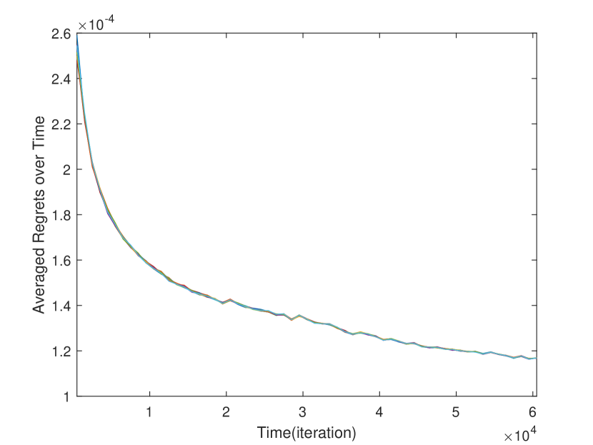
(b) The temporal average of regret converges to zero for all agents.

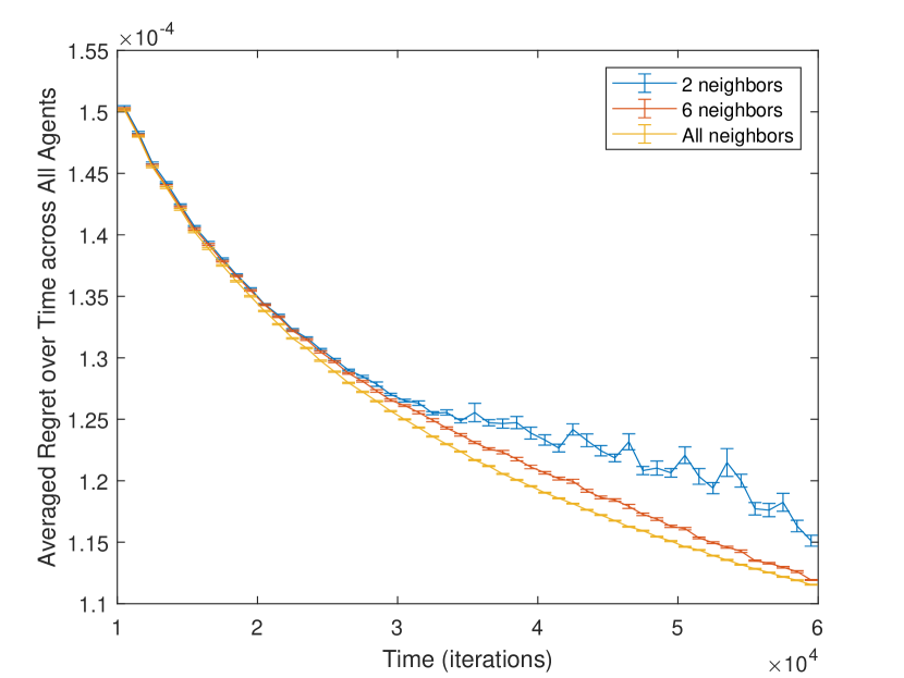
(c) The averaged regrets over time for different networks: more connectivity results in smaller regret.

Figure 1: The individual regrets of all agents are shown to be sublinear.

Remark 3.

The exact expression of regret (given in (43)) shows its dependence to $(1-\beta)^{-1}$, where $\beta$ is the second largest singular value of $\mathbf{P}$. This implies that when the network is well-connected (i.e., $\beta$ is smaller), the resulting bound is tighter. A smaller $\beta$ allows the Markov chain $\mathbf{P}$ to mix faster, which intuitively results in faster information propagation over the network of agents.

III-C Key Technical Challenges in the Proof

The regret can be decomposed into three terms, where each term must be small enough to bound the regret. In [4], two of these terms are bounded using the properties of strong stability and sequential strong stability, and one term is bounded using the standard regret bound for online gradient descent. In our setup, since $(\mathbf{A},\mathbf{B})$ is unknown, the agents cannot work with the ideal feasible set in (4), and as evident from line 25 of the algorithm, $\mathcal{S}^{i}_{t+1}$ is constructed only based on agent $i$ system estimate. This brings forward two challenges. (i) Agent $i$ constructs the controllers based on iterates $\Sigma_{i,t+1}$ that are not necessarily in the feasible set of (4), so we need to establish the stability properties of these controllers. (ii) The feasible sets are different across agents (i.e., $\mathcal{S}^{i}_{t+1}\neq\mathcal{S}^{j}_{t+1}$ for $i\neq j$), so we cannot directly apply distributed online optimization results on a common feasible set.

To tackle the first challenge, we first derive the bound on the precision of each agent system estimate based on the EXTRA algorithm (see Lemma 6) and combine that with statistical properties of centralized LS estimation using results of [8]. We then establish that if each agent system estimate is close enough to the true system, a strongly stable policy w.r.t. the system estimate is also strongly stable w.r.t. the true system (see Lemma 3 and Lemma 4). To address the second challenge, we use alternating projections to prove that a point in the feasible set of one agent is close enough to its projection to the feasible set of another agent, when estimates of these two agents are close. Then, in Theorem 9, we show the contribution of distributed online optimization to the regret. We finally put together these results to prove our regret bound.

IV Numerical Experiments

We now provide numerical simulations verifying the theoretical guarantee of our algorithm.

Experiment Setup: We first consider a network of $m=20$ agents, captured by a cyclic graph, where each agent has a self-weight of 0.6 and assigns the weight 0.2 to each of its two neighbors. The (hyper)-parameters are set as follows: $d=k=3$, $\kappa=1.5$, $\gamma=0.4$, $C=300$. We let matrices $\mathbf{A}=(1-2\gamma)\mathbf{I}$ and $\mathbf{B}=(\gamma/\kappa)\mathbf{I}$ to ensure the existence of a $(\kappa,\gamma)$-strongly stable controller. For time-varying cost matrices, we set $\mathbf{Q}_{i,t}$ (respectively, $\mathbf{R}_{i,t}$) as a diagonal matrix where each diagonal term is sampled from the uniform distribution over $[0,C/d]$ (respectively, $[0,C/k]$), so that $\text{Tr}(\mathbf{Q}_{i,t}),\text{Tr}(\mathbf{R}_{i,t})\leq C$. The disturbance $\mathbf{w}_{i,t}$ is sampled from a standard Gaussian distribution, and thus $\lambda^{2}=d=3$ and $\sigma^{2}=1$.

Simulation: We simulate Algorithm 1 for $T=1K,2K,3K,\ldots,60K$. For the benchmark, we set $\mathbf{K}^{s}$ as $(-\kappa)10^{-2}\mathbf{I}$ which is $(\kappa,\gamma)$-strongly stable w.r.t. $\mathbf{A},\mathbf{B}$, and the resulting cumulative cost is small enough to be the benchmark. For the projection on the feasible set, we apply Dykstra’s projection algorithm. Due to floating-point computations, $\mathbf{V}_{i,t}$ for action-sampling may not be positive semi-definite (PSD). Therefore, we address it by adding to $\mathbf{V}_{i,t}$ a small term ($(1e-15)\mathbf{I}$) to keep it PSD. The entire process is repeated for $50$ Monte-Carlo simulations, and in the figures we present the averaged plots.

Iterations	20K	30K	40K	50K	60K
Averaged Regret	1.424	1.34	1.248	1.201	1.168
Standard Error	0.0087	0.0097	0.0052	0.0032	0.0037

TABLE I: The mean and standard error of the averaged regret over time and agents ($\times 10^{-4}$).

Performance: I) Sublinearity of Regret: To verify the result of Theorem 2, in Fig. 1(b), we present the averaged regret over time (i.e., individual regret divided by $T$), which is clearly decreasing over time. In Table I, we tabulate the averaged regrets (over time and agents) as well as their standard errors computed from $50$ trials for $T=20K,30K,40K,50K,60K$. We can see that $50$ trials is enough to obtain a small standard error. II) Impact of Network Topology: To study the impact of network topology, we use three different networks: a cyclic graph with 2 neighbors (Net A), a cyclic graph with 6 neighbors (Net B) and a complete graph (Net C) where every entry of $\mathbf{P}$ is $\frac{1}{20}$. From Fig. 1(c), we can see that the regret increases when $\beta$ is smaller (Net A $>$ Net B $>$ Net C). This result is consistent with Remark 3 on the impact of $\beta$.

V Conclusion

In this paper, we considered the distributed online LQR problem with unknown LTI systems and time-varying quadratic cost functions. We developed a fully decentralized algorithm to estimate the unknown system and minimize the finite-horizon cost, which can be cast as a regret minimization. We proved that the individual regret, which is the performance of the control sequence of any agent compared to the best (linear and strongly stable) controller in hindsight, is upper bounded by $O(T^{2/3}\log T)$. Future directions include analyzing the dynamic regret defined w.r.t. the optimal (instantaneous) control policy in hindsight, investigating coupled time-varying cost functions, and analyzing the adversarial noise setup.

VI Appendix

Let us start with an outline of the appendix as follows.

1. In Section VI-A, we discuss the connection of strong stability for two close enough LTI systems. We further discuss the relation between the steady-state covariance matrices of these systems.

2. In Section VI-B, based on the results in [8] and the EXTRA algorithm [9], we quantify the precision of the system estimate of each agent.

3. As mentioned in the proof sketch, there is a term in the regret decomposition, related to distributed online optimization with different feasible sets across agents. In Section VI-C, we provide auxiliary lemmas to bound this term in Theorem 9.

4. In Section VI-D, we prove our main result (Theorem 2) by putting together the above results.

VI-A Strong Stability of Two Similar LTI Systems

Notice that we deal with a problem with unknown system dynamics, where each agent decides its control signal based on its own system estimates. Therefore, we should quantify how a strongly stable controller w.r.t. one system performs on another similar system, and how two steady-state covariance matrices of these two systems are related to each other.

Lemma 3.

A linear policy $\mathbf{K}$ which is $(\kappa,\gamma)$-strongly stable ($\kappa\geq 1$) for the LTI system $(\mathbf{A}_{1},\mathbf{B}_{1})$, is also $(\kappa,\gamma-2\kappa^{2}\epsilon)$-strongly stable for the LTI system $(\mathbf{A}_{2},\mathbf{B}_{2})$ if $\lVert[\mathbf{A}_{1}\>\mathbf{B}_{1}]-[\mathbf{A}_{2}\>\mathbf{B}_{2}]\rVert_{F}\leq\epsilon$ and $\epsilon<\frac{\gamma}{2\kappa^{2}}$.

Proof.

Based on the definition of strong stability, we have $\mathbf{A}_{1}+\mathbf{B}_{1}\mathbf{K}=\mathbf{H}\mathbf{L}\mathbf{H}^{-1}$ with $\lVert\mathbf{H}\rVert\lVert\mathbf{H}^{-1}\rVert\leq\kappa$ and $\lVert\mathbf{L}\rVert\leq 1-\gamma$. Therefore, we have

$$\begin{split}&\mathbf{A}_{2}+\mathbf{B}_{2}\mathbf{K}\\ =&\mathbf{A}_{1}+\mathbf{B}_{1}\mathbf{K}+(\mathbf{A}_{2}-\mathbf{A}_{1})+(\mathbf{B}_{2}-\mathbf{B}_{1})\mathbf{K}\\ =&\mathbf{H}\mathbf{L}\mathbf{H}^{-1}+\mathbf{H}\mathbf{H}^{-1}[(\mathbf{A}_{2}-\mathbf{A}_{1})+(\mathbf{B}_{2}-\mathbf{B}_{1})\mathbf{K}]\mathbf{H}\mathbf{H}^{-1}\\ =&\mathbf{H}\big{[}\mathbf{L}+\mathbf{H}^{-1}[(\mathbf{A}_{2}-\mathbf{A}_{1})+(\mathbf{B}_{2}-\mathbf{B}_{1})\mathbf{K}]\mathbf{H}\big{]}\mathbf{H}^{-1}.\end{split}$$

For the middle term, it can be shown that

$$\begin{split}&\lVert\mathbf{L}+\mathbf{H}^{-1}[(\mathbf{A}_{2}-\mathbf{A}_{1})+(\mathbf{B}_{2}-\mathbf{B}_{1})\mathbf{K}]\mathbf{H}\rVert\\ \leq&\lVert\mathbf{L}\rVert+\lVert\mathbf{H}^{-1}\rVert\lVert(\mathbf{A}_{2}-\mathbf{A}_{1})+(\mathbf{B}_{2}-\mathbf{B}_{1})\mathbf{K}\rVert\lVert\mathbf{H}\rVert\\ \leq&(1-\gamma)+\kappa(\lVert\mathbf{A}_{2}-\mathbf{A}_{1}\rVert+\lVert(\mathbf{B}_{2}-\mathbf{B}_{1})\mathbf{K}\rVert)\\ \leq&(1-\gamma)+\kappa(\epsilon+\epsilon\kappa)\\ \leq&(1-\gamma)+2\kappa^{2}\epsilon.\end{split}$$

Since $\gamma-2\kappa^{2}\epsilon>0$, based on the result above, we can see that the policy $\mathbf{K}$ is $(\kappa,\gamma-2\kappa^{2}\epsilon)$-strongly stable w.r.t. the LTI system $(\mathbf{A}_{2},\mathbf{B}_{2})$ as $\mathbf{A}_{2}+\mathbf{B}_{2}\mathbf{K}=\mathbf{H}\mathbf{L}_{2}\mathbf{H}^{-1}$ where $\mathbf{L}_{2}:=\mathbf{L}+\mathbf{H}^{-1}[(\mathbf{A}_{2}-\mathbf{A}_{1})+(\mathbf{B}_{2}-\mathbf{B}_{1})\mathbf{K}]\mathbf{H}$ and $\lVert\mathbf{L}_{2}\rVert\leq 1-(\gamma-2\kappa^{2}\epsilon)$. ∎

Lemma 4.

Given a linear policy $\mathbf{K}$ which is $(\kappa,\gamma)$-strongly stable ($\kappa\geq 1$) for the LTI system $(\mathbf{A}_{1},\mathbf{B}_{1})$, if $\lVert[\mathbf{A}_{1}\>\mathbf{B}_{1}]-[\mathbf{A}_{2}\>\mathbf{B}_{2}]\rVert_{F}\leq\epsilon$ and $\epsilon<\frac{\gamma}{2\kappa^{2}}$, we have that

$$\mathbf{X}_{1}\succeq\mathbf{X}_{2}-4\kappa^{6}\text{Tr}(\mathbf{W})\frac{\epsilon[1-(\gamma-2\kappa^{2}\epsilon)]}{(\gamma-2\kappa^{2}\epsilon)(1-(1-\gamma)^{2})}\cdot\mathbf{I},$$

where $\mathbf{X}_{1}(\text{respectively},\mathbf{X}_{2})$ is the steady-state covariance matrix obtained by applying the controller $\mathbf{u}_{t}=\mathbf{K}\mathbf{x}_{t}$ on the system $\mathbf{x}_{t+1}=\mathbf{A}_{1}\mathbf{x}_{t}+\mathbf{B}_{1}\mathbf{u}_{t}+\mathbf{w}_{t}$ (respectively, $\mathbf{x}_{t+1}=\mathbf{A}_{2}\mathbf{x}_{t}+\mathbf{B}_{2}\mathbf{u}_{t}+\mathbf{w}_{t}$).

Proof.

Based on Lemma 3, we know that the policy $\mathbf{K}$ is $(\kappa,\gamma)$ and $(\kappa,\gamma-2\kappa^{2}\epsilon)$-strongly stable for the systems $(\mathbf{A}_{1},\mathbf{B}_{1})$ and $(\mathbf{A}_{2},\mathbf{B}_{2})$, respectively. We then have

$$\begin{split}\mathbf{X}_{1}&=(\mathbf{A}_{1}+\mathbf{B}_{1}\mathbf{K})\mathbf{X}_{1}(\mathbf{A}_{1}+\mathbf{B}_{1}\mathbf{K})^{\top}+\mathbf{W},\\ \mathbf{X}_{2}&=(\mathbf{A}_{2}+\mathbf{B}_{2}\mathbf{K})\mathbf{X}_{2}(\mathbf{A}_{2}+\mathbf{B}_{2}\mathbf{K})^{\top}+\mathbf{W}.\end{split}$$

Denoting $\Delta:=\mathbf{X}_{1}-\mathbf{X}_{2}$, we get

$$\begin{split}&\mathbf{X}_{2}+\Delta\\ =&(\mathbf{A}_{1}+\mathbf{B}_{1}\mathbf{K})(\mathbf{X}_{2}+\Delta)(\mathbf{A}_{1}+\mathbf{B}_{1}\mathbf{K})^{\top}+\mathbf{W}\\ =&(\mathbf{A}_{2}+\mathbf{B}_{2}\mathbf{K})\mathbf{X}_{2}(\mathbf{A}_{2}+\mathbf{B}_{2}\mathbf{K})^{\top}\\ +&[(\mathbf{A}_{1}+\mathbf{B}_{1}\mathbf{K})-(\mathbf{A}_{2}+\mathbf{B}_{2}\mathbf{K})]\mathbf{X}_{2}(\mathbf{A}_{2}+\mathbf{B}_{2}\mathbf{K})^{\top}\\ +&(\mathbf{A}_{2}+\mathbf{B}_{2}\mathbf{K})\mathbf{X}_{2}[(\mathbf{A}_{1}+\mathbf{B}_{1}\mathbf{K})-(\mathbf{A}_{2}+\mathbf{B}_{2}\mathbf{K})]^{\top}\\ +&[\mathbf{A}_{1}-\mathbf{A}_{2}+(\mathbf{B}_{1}-\mathbf{B}_{2})\mathbf{K}]\mathbf{X}_{2}[\mathbf{A}_{1}-\mathbf{A}_{2}+(\mathbf{B}_{1}-\mathbf{B}_{2})\mathbf{K}]^{\top}\\ +&(\mathbf{A}_{1}+\mathbf{B}_{1}\mathbf{K})\Delta(\mathbf{A}_{1}+\mathbf{B}_{1}\mathbf{K})^{\top}+\mathbf{W}.\end{split}$$

From the equation above, we have

$$\begin{split}&\Delta\\ =&[(\mathbf{A}_{1}+\mathbf{B}_{1}\mathbf{K})-(\mathbf{A}_{2}+\mathbf{B}_{2}\mathbf{K})]\mathbf{X}_{2}(\mathbf{A}_{2}+\mathbf{B}_{2}\mathbf{K})^{\top}\\ +&(\mathbf{A}_{2}+\mathbf{B}_{2}\mathbf{K})\mathbf{X}_{2}[(\mathbf{A}_{1}+\mathbf{B}_{1}\mathbf{K})-(\mathbf{A}_{2}+\mathbf{B}_{2}\mathbf{K})]^{\top}\\ +&[\mathbf{A}_{1}-\mathbf{A}_{2}+(\mathbf{B}_{1}-\mathbf{B}_{2})\mathbf{K}]\mathbf{X}_{2}[\mathbf{A}_{1}-\mathbf{A}_{2}+(\mathbf{B}_{1}-\mathbf{B}_{2})\mathbf{K}]^{\top}\\ +&(\mathbf{A}_{1}+\mathbf{B}_{1}\mathbf{K})\Delta(\mathbf{A}_{1}+\mathbf{B}_{1}\mathbf{K})^{\top}\\ \succeq&[(\mathbf{A}_{1}+\mathbf{B}_{1}\mathbf{K})-(\mathbf{A}_{2}+\mathbf{B}_{2}\mathbf{K})]\mathbf{X}_{2}(\mathbf{A}_{2}+\mathbf{B}_{2}\mathbf{K})^{\top}\\ +&(\mathbf{A}_{2}+\mathbf{B}_{2}\mathbf{K})\mathbf{X}_{2}[(\mathbf{A}_{1}+\mathbf{B}_{1}\mathbf{K})-(\mathbf{A}_{2}+\mathbf{B}_{2}\mathbf{K})]^{\top}\\ +&(\mathbf{A}_{1}+\mathbf{B}_{1}\mathbf{K})\Delta(\mathbf{A}_{1}+\mathbf{B}_{1}\mathbf{K})^{\top}.\end{split}$$

Denoting

$$\begin{split}\Psi&:=[(\mathbf{A}_{1}+\mathbf{B}_{1}\mathbf{K})-(\mathbf{A}_{2}+\mathbf{B}_{2}\mathbf{K})]\mathbf{X}_{2}(\mathbf{A}_{2}+\mathbf{B}_{2}\mathbf{K})^{\top}\\ +&(\mathbf{A}_{2}+\mathbf{B}_{2}\mathbf{K})\mathbf{X}_{2}[(\mathbf{A}_{1}+\mathbf{B}_{1}\mathbf{K})-(\mathbf{A}_{2}+\mathbf{B}_{2}\mathbf{K})]^{\top}\end{split}$$

and applying the inequality above recursively, we get

$$\begin{split}\Delta&\succeq\Psi+(\mathbf{A}_{1}+\mathbf{B}_{1}\mathbf{K})\Psi(\mathbf{A}_{1}+\mathbf{B}_{1}\mathbf{K})^{\top}+\ldots\\ &+(\mathbf{A}_{1}+\mathbf{B}_{1}\mathbf{K})^{n}\Psi((\mathbf{A}_{1}+\mathbf{B}_{1}\mathbf{K})^{\top})^{n}\\ &+(\mathbf{A}_{1}+\mathbf{B}_{1}\mathbf{K})^{n+1}\Delta((\mathbf{A}_{1}+\mathbf{B}_{1}\mathbf{K})^{\top})^{n+1}.\end{split}$$

As $n\rightarrow\infty$, the spectral norm of the right hand side is upper bounded by $\kappa^{2}\lVert\Psi\rVert/[1-(1-\gamma)^{2}]$, which implies

$$\Delta\succeq\frac{-\kappa^{2}\lVert\Psi\rVert}{1-(1-\gamma)^{2}}\mathbf{I}.$$ (5)

We also have

$$\begin{split}\lVert\Psi\rVert\leq&2\lVert(\mathbf{A}_{1}+\mathbf{B}_{1}\mathbf{K})-(\mathbf{A}_{2}+\mathbf{B}_{2}\mathbf{K})\rVert\lVert\mathbf{X}_{2}\rVert\lVert\mathbf{A}_{2}+\mathbf{B}_{2}\mathbf{K}\rVert\\ \leq&2(2\kappa\epsilon)[\kappa(1-(\gamma-2\kappa^{2}\epsilon))]\lVert\mathbf{X}_{2}\rVert\\ \leq&4\kappa^{2}\epsilon(1-(\gamma-2\kappa^{2}\epsilon))\frac{\kappa^{2}}{\gamma-2\kappa^{2}\epsilon}\text{Tr}(\mathbf{W}),\end{split}$$

where the second inequality is due to the strong stability of $\mathbf{K}$ w.r.t. $(\mathbf{A}_{2},\mathbf{B}_{2})$ and the third inequality is derived by applying Lemma 3.3 in [4]. Substituting the above upper bound into (5), the result is proved. ∎

Corollary 5.

Given a linear policy $\mathbf{K}$ which is $(\kappa,\gamma)$-strongly stable ($\kappa\geq 1$) for the LTI system $(\mathbf{A}_{1},\mathbf{B}_{1})$, if $\lVert[\mathbf{A}_{1}\>\mathbf{B}_{1}]-[\mathbf{A}_{2}\>\mathbf{B}_{2}]\rVert_{F}\leq\epsilon$ and $\epsilon\leq\frac{\gamma}{4\kappa^{2}}$, we have the following result:

$$\mathbf{X}_{1}\succeq\mathbf{X}_{2}-\xi\epsilon\cdot\mathbf{I},$$

where $\xi:=\text{Tr}(\mathbf{W})\frac{4\kappa^{6}}{\gamma^{2}}$.

VI-B Precision of the System Estimates

Since the final regret bound depends on the precision of all agents system estimates, in this section we show that with a specific choice of $T_{0}$ (iterations for collecting data), $T_{1}$ (iterations for performing EXTRA) and $T$, the precision of each agent estimate and the distance between any two agents estimates are upper bounded by $O(T^{-1/3})$.

Lemma 6.

Assume $\lVert[\mathbf{A}\>\mathbf{B}]\rVert_{F}\leq\vartheta$ and apply Algorithm 1 with $T_{0}=T^{2/3}\log(T/\delta)$ and $T_{1}=O(\log(T^{1/3}))$ and $T_{0}\geq\max\{200(\log(12^{n})+\log(\frac{3m}{\delta})),4\varrho+6m+3d\}$, where $\varrho:=\frac{m144\vartheta^{2}\kappa_{0}^{4}}{\gamma_{0}^{2}}(1+\vartheta^{2}\kappa_{0}^{2})$. Then, for $t,t^{\prime}\in\{T_{s},\ldots,T\}$ and $i,j\in[m]$, with probability $(1-\delta)$, we have

$$\lVert[\widehat{\mathbf{A}}_{i,t}\>\widehat{\mathbf{B}}_{i,t}]-[\mathbf{A}\>\mathbf{B}]\rVert_{F}\leq(1+\frac{38\sqrt{2}n}{\sqrt{m}})T^{-1/3},$$

and

$$\lVert[\widehat{\mathbf{A}}_{i,t}\>\widehat{\mathbf{B}}_{i,t}]-[\widehat{\mathbf{A}}_{j,t^{\prime}}\>\widehat{\mathbf{B}}_{j,t^{\prime}}]\rVert_{F}\leq 2T^{-1/3}.$$

Proof.

Let $V_{0}:=\sum_{i=1}^{m}\sum_{t=1}^{T_{0}}\mathbf{z}_{i,t}\mathbf{z}_{i,t}^{\top}$. Based on Theorem 20 in [8], we have the following relationships:

• With probability at least $(1-\delta/3)$,

  $$\text{Tr}(V_{0})\leq(mT_{0})\frac{144\sigma^{2}\kappa_{0}^{4}}{\gamma_{0}^{2}}(n+k\vartheta^{2}\kappa_{0}^{2})\log(\frac{6mT_{0}}{\delta}).$$ (6)

• With probability at least $(1-\delta/3)$, based on our choice of $T_{0}$, we have that

  $$V_{0}\succeq\frac{mT_{0}\sigma^{2}}{80}\mathbf{I}.$$ (7)

• By solving the following LS problem

  $$\min_{[\mathbf{A},\mathbf{B}]}\sum_{i=1}^{m}\sum_{t=1}^{T_{0}}\lVert[\mathbf{A}\>\mathbf{B}]\mathbf{z}_{i,t}-\mathbf{x}_{i,t+1}\rVert^{2}+\sigma^{2}\vartheta^{-2}\lVert[\mathbf{A}\>\mathbf{B}]\rVert^{2},$$

  where the estimates $[\widehat{\mathbf{A}}\>\widehat{\mathbf{B}}]=(\sum_{i=1}^{m}\sum_{t=1}^{T_{0}}\mathbf{x}_{i,t+1}\mathbf{z}_{i,t}^{\top})V^{-1}$ and $V=V_{0}+\sigma^{2}\vartheta^{-2}\mathbf{I}$, we have with probability at least $(1-\delta/3)$ (based on our choice of $T_{0}$)

  $$\text{Tr}(\widehat{\Delta}V\widehat{\Delta}^{\top})\leq 18\sigma^{2}n^{2}\log(T_{0}/\delta),$$ (8)

  where $\widehat{\Delta}=[\widehat{\mathbf{A}}\>\widehat{\mathbf{B}}]-[\mathbf{A}\>\mathbf{B}]$.

Combining (7) and (8), we get

$$\lVert\widehat{\Delta}\rVert_{F}\leq\frac{38n}{\sqrt{m}}\sqrt{\frac{\log(T_{0}/\delta)}{T_{0}}}.$$

Since $T_{0}=T^{2/3}\log(T/\delta)$, we have

$$\lVert\widehat{\Delta}\rVert_{F}\leq\frac{38\sqrt{2}n}{\sqrt{m}}T^{-1/3}.$$ (9)

After the first $(T_{0}+1)$ iterations, we apply the EXTRA algorithm [9], and based on Theorem 3.7 in [9], we have the upper bound of the distance between $(\widehat{\mathbf{A}}_{i,t},\widehat{\mathbf{B}}_{i,t})$ (agent $i$ estimation at iteration $t$) and $(\widehat{\mathbf{A}},\widehat{\mathbf{B}})$, the solution of the global function $f(\mathbf{A},\mathbf{B})=\sum_{i=1}^{m}f_{i}(\mathbf{A},\mathbf{B})$ as follows. There exists $0<\tau<1$ such that

$$\lVert[\widehat{\mathbf{A}}_{i,t}\>\widehat{\mathbf{B}}_{i,t}]-[\widehat{\mathbf{A}}\>\widehat{\mathbf{B}}]\rVert_{F}\leq\phi\tau^{t-(T_{0}+1)},\;\forall i,$$ (10)

where $\phi$ is a constant. Based on (9), (10) and our choice of $T_{1}$ ($T_{1}=(-\log\tau)^{-1}\log(\phi T^{1/3})$), for $t\in[T_{s},\ldots,T]$ and $i,j\in[m]$, we have

$$\begin{split}\lVert[\widehat{\mathbf{A}}_{i,t}\>\widehat{\mathbf{B}}_{i,t}]-[\mathbf{A}\>\mathbf{B}]\rVert_{F}&\leq\lVert[\widehat{\mathbf{A}}_{i,t}\>\widehat{\mathbf{B}}_{i,t}]-[\widehat{\mathbf{A}}\>\widehat{\mathbf{B}}]\rVert_{F}+\lVert\widehat{\Delta}\rVert_{F}\\ \leq&(1+\frac{38\sqrt{2}n}{\sqrt{m}})T^{-1/3},\end{split}$$ (11)

and

$$\begin{split}&\lVert[\widehat{\mathbf{A}}_{i,t}\>\widehat{\mathbf{B}}_{i,t}]-[\widehat{\mathbf{A}}_{j,t^{\prime}}\>\widehat{\mathbf{B}}_{j,t^{\prime}}]\rVert_{F}\\ \leq&\lVert[\widehat{\mathbf{A}}_{i,t}\>\widehat{\mathbf{B}}_{i,t}]-[\widehat{\mathbf{A}}\>\widehat{\mathbf{B}}]\rVert_{F}+\lVert[\widehat{\mathbf{A}}_{j,t^{\prime}}\>\widehat{\mathbf{B}}_{j,t^{\prime}}]-[\widehat{\mathbf{A}}\>\widehat{\mathbf{B}}]\rVert_{F}\\ \leq&2T^{-1/3}.\end{split}$$ (12)

∎

VI-C Bound of the Distributed Online SDP

From the line 25 of Algorithm 1, we can see that the feasible set of SDP for each agent is based on the agent system estimate, so we cannot directly apply distributed online optimization results on a common feasible set. Here, we provide auxiliary results to bound the error due to distributed online optimization. In Lemma 8, we use alternating projections to prove that a point in the feasible set of one agent is close enough to its projection to the feasible set of another agent, when estimates of these two agents are close. Then, in Theorem 9, we show the contribution of distributed online optimization to the regret.

Lemma 7.

Consider an affine set $\mathcal{H}=\{\mathbf{x}|\mathbf{E}\mathbf{x}=\mathbf{w}\}$, where $\mathbf{E}\in\mathbf{R}^{m\times n}$ is full row rank and $n>m$. For two points $\mathbf{p}_{1},\mathbf{p}_{2}$, we have the following relationships.
(i) $\lVert\Pi_{\mathcal{H}}(\mathbf{p}_{1})-\Pi_{\mathcal{H}}(\mathbf{p}_{2})\rVert<\lVert\mathbf{p}_{1}-\mathbf{p}_{2}\rVert$ if $(\mathbf{p}_{1}-\mathbf{p}_{2})$ is not in the null space of $\mathbf{E}$.
(ii) $\lVert\mathbf{p}_{1}-\Pi_{\mathcal{H}}(\mathbf{p}_{1})\rVert=\lVert\mathbf{p}_{2}-\Pi_{\mathcal{H}}(\mathbf{p}_{2})\rVert$ if $(\mathbf{p}_{1}-\mathbf{p}_{2})$ is in the null space of $\mathbf{E}$.

Proof.

The orthogonal projection to affine set has the following closed-form [52]

$$\Pi_{\mathcal{H}}(\mathbf{p}_{1})=[\mathbf{I}-\mathbf{E}^{\top}(\mathbf{E}\mathbf{E}^{\top})^{-1}\mathbf{E}]\mathbf{p}_{1}+\mathbf{E}^{\top}(\mathbf{E}\mathbf{E}^{\top})^{-1}\mathbf{w}.$$ (13)

The proof then follows immediately. ∎

Lemma 8.

Suppose two system estimates $(\widehat{\mathbf{A}}_{1},\widehat{\mathbf{B}}_{1})$ and $(\widehat{\mathbf{A}}_{2},\widehat{\mathbf{B}}_{2})$ such that $\lVert[\widehat{\mathbf{A}}_{1}\;\widehat{\mathbf{B}}_{1}]-[\widehat{\mathbf{A}}_{2}\;\widehat{\mathbf{B}}_{2}]\rVert_{F}\leq\epsilon_{1}$, and $\lVert[\widehat{\mathbf{A}}_{1}\;\widehat{\mathbf{B}}_{1}]-[\mathbf{A}\;\mathbf{B}]\rVert_{F},\lVert[\widehat{\mathbf{A}}_{2}\;\widehat{\mathbf{B}}_{2}]-[\mathbf{A}\;\mathbf{B}]\rVert_{F}\leq\epsilon_{2}$. Let us denote $\mathcal{D}:=\{\Sigma|\Sigma\succeq 0,\text{Tr}(\Sigma)\leq\nu\}$ and represent

$$\mathcal{H}_{1} :=\{\Sigma_{\mathbf{x}\mathbf{x}}=\widehat{\mathbf{C}}_{1}\Sigma\widehat{\mathbf{C}}_{1}^{\top}+\mathbf{W}\}~{}~{}~{}~{}\widehat{\mathbf{C}}_{1}:=[\widehat{\mathbf{A}}_{1}\;\widehat{\mathbf{B}}_{1}]$$

$$\mathcal{H}_{2} :=\{\Sigma_{\mathbf{x}\mathbf{x}}=\widehat{\mathbf{C}}_{2}\Sigma\widehat{\mathbf{C}}_{2}^{\top}+\mathbf{W}\}~{}~{}~{}~{}\widehat{\mathbf{C}}_{2}:=[\widehat{\mathbf{A}}_{2}\;\widehat{\mathbf{B}}_{2}].$$

Let us also define $\mathcal{S}_{1}:=\mathcal{D}\cap\mathcal{H}_{1}$ and $\mathcal{S}_{2}:=\mathcal{D}\cap\mathcal{H}_{2}$, respectively. Then, for any point $\Sigma_{1}\in\mathcal{S}_{1}$, we have that $\lVert\Sigma_{1}-\Pi_{\mathcal{S}_{2}}(\Sigma_{1})\rVert$ is $O(\epsilon_{1})$.

Proof.

We can see that $\mathcal{H}_{1}$ can we written as

$$\begin{bmatrix}\mathbf{I}&\mathbf{0}\end{bmatrix}\Sigma\begin{bmatrix}\mathbf{I}\\ \mathbf{0}\end{bmatrix}=\widehat{\mathbf{C}}_{1}\Sigma\widehat{\mathbf{C}}_{1}^{\top}+\mathbf{W}.$$

Denoting $\mathbf{D}:=[\mathbf{I}\;\mathbf{0}]$, we have the vectorized version of the linear system above as

$$(\mathbf{D}\otimes\mathbf{D}-\widehat{\mathbf{C}}_{1}\otimes\widehat{\mathbf{C}}_{1})\text{vec}(\Sigma)=\text{vec}(\mathbf{W}),$$

and we let $\mathbf{E}_{1}:=\mathbf{D}\otimes\mathbf{D}-\widehat{\mathbf{C}}_{1}\otimes\widehat{\mathbf{C}}_{1}$. Similarly, we can write $\mathcal{H}_{2}$ as $(\mathbf{E}_{2})\text{vec}(\Sigma)=\text{vec}(\mathbf{W})$. For the rest of the proof, we consider $\Sigma_{1}$ as $\text{vec}(\Sigma_{1})$. Supposing both $\mathbf{E}_{1}$ and $\mathbf{E}_{2}$ are full row rank and applying (13), for any point $\Sigma_{1}\in\mathcal{S}_{1}$ we have

$$\begin{split}&\Sigma_{1}-\Pi_{\mathcal{H}_{2}}(\Sigma_{1})=\mathbf{E}_{2}^{\top}(\mathbf{E}_{2}\mathbf{E}_{2}^{\top})^{-1}(\mathbf{E}_{2}-\mathbf{E}_{1})\Sigma_{1}.\end{split}$$ (14)

We know that $\Sigma_{1}\in\mathcal{S}_{1}$ and $[\widehat{\mathbf{A}}_{2}\;\widehat{\mathbf{B}}_{2}]$ has a finite norm, so there exists a constant upper-bounding $\lVert\mathbf{E}_{2}^{\top}(\mathbf{E}_{2}\mathbf{E}_{2}^{\top})^{-1}\rVert\lVert\Sigma_{1}\rVert$. To show $\lVert\Sigma_{1}-\Pi_{\mathcal{H}_{2}}(\Sigma_{1})\rVert$ is $O(\epsilon_{1})$, it is sufficient to show $\lVert\mathbf{E}_{1}-\mathbf{E}_{2}\rVert$ is $O(\epsilon_{1})$. Based on the expressions of $\mathbf{E}_{1}$ and $\mathbf{E}_{2}$, we have that

$$\begin{split}&\lVert\mathbf{E}_{2}-\mathbf{E}_{1}\rVert\\ =&\lVert\widehat{\mathbf{C}}_{2}\otimes\widehat{\mathbf{C}}_{2}-\widehat{\mathbf{C}}_{1}\otimes\widehat{\mathbf{C}}_{1}\rVert\\ \leq&\lVert\widehat{\mathbf{C}}_{2}\otimes\widehat{\mathbf{C}}_{2}-\widehat{\mathbf{C}}_{2}\otimes\widehat{\mathbf{C}}_{1}+\widehat{\mathbf{C}}_{2}\otimes\widehat{\mathbf{C}}_{1}-\widehat{\mathbf{C}}_{1}\otimes\widehat{\mathbf{C}}_{1}\rVert_{F}\\ \leq&(\lVert\widehat{\mathbf{C}}_{1}\rVert_{F}+\lVert\widehat{\mathbf{C}}_{2}\rVert_{F})\lVert\widehat{\mathbf{C}}_{2}-\widehat{\mathbf{C}}_{1}\rVert_{F},\end{split}$$ (15)

which shows that $\lVert\mathbf{E}_{2}-\mathbf{E}_{1}\rVert$ is $O(\epsilon_{1})$ due to the assumption that $\lVert\widehat{\mathbf{C}}_{2}-\widehat{\mathbf{C}}_{1}\rVert_{F}=\epsilon_{1}$. Therefore, we conclude that there exists a constant $\theta$ such that $\lVert\Sigma_{1}-\Pi_{\mathcal{H}_{2}}(\Sigma_{1})\rVert\leq\theta\epsilon_{1}$.

$\mathcal{S}_{1}$ and $\mathcal{S}_{2}$ are both non-empty and neither is a singleton. For any point $\Sigma_{1}\in\mathcal{S}_{1}$, if $\Pi_{\mathcal{H}_{2}}(\Sigma_{1})\in\mathcal{D}$, by (14) and Pythagorean theorem, we have

$$\lVert\Sigma_{1}-\Pi_{\mathcal{S}_{2}}(\Sigma_{1})\rVert\leq\lVert\Sigma_{1}-\Pi_{\mathcal{H}_{2}}(\Sigma_{1})\rVert\leq\theta\epsilon_{1},$$ (16)

and the claim of lemma holds immediately. If $\Pi_{\mathcal{H}_{2}}(\Sigma_{1})\notin\mathcal{D}$, we consider the process of applying alternating projections for $\Sigma_{1}$ on $\mathcal{S}_{2}$. Let $\mathbf{y}_{0}=\Sigma_{1}$ and consider the following iterates

$$\Pi_{\mathcal{D}}(\mathbf{a}_{k-1})=\mathbf{y}_{k}~{}~{}~{}~{}\Pi_{\mathcal{H}_{2}}(\mathbf{y}_{k})=\mathbf{a}_{k},\>k=1,2,3,\ldots,$$ (17)

where we denote the limit point by $\Sigma_{1}^{\prime}$. For the above sequences, based on the definition of projection we have

$$\lVert\mathbf{y}_{k+1}-\mathbf{a}_{k}\rVert^{2}=\lVert\mathbf{y}_{k+1}-\mathbf{a}_{k+1}\rVert^{2}+\lVert\mathbf{a}_{k+1}-\mathbf{a}_{k}\rVert^{2},$$

which implies

$$\begin{split}\lVert\mathbf{y}_{k+1}-\mathbf{a}_{k+1}\rVert^{2}&=\lVert\mathbf{y}_{k+1}-\mathbf{a}_{k}\rVert^{2}-\lVert\mathbf{a}_{k+1}-\mathbf{a}_{k}\rVert^{2}\\ &\leq\lVert\mathbf{y}_{k}-\mathbf{a}_{k}\rVert^{2}-\lVert\mathbf{a}_{k+1}-\mathbf{a}_{k}\rVert^{2}.\end{split}$$ (18)

Without loss of generality, we assume $\lVert\mathbf{a}_{k+1}-\mathbf{a}_{k}\rVert>0$ for all $k$. If $\lVert\mathbf{a}_{k+1}-\mathbf{a}_{k}\rVert=0$ at $k=\tilde{k}$, the sequence has converged in a finite number of steps (i.e., $\mathbf{a}_{k}=\mathbf{y}_{k}=\Sigma_{1}^{\prime}$ for $k\geq\tilde{k}$), and the following proof still holds. Assuming $\lVert\mathbf{a}_{k+1}-\mathbf{a}_{k}\rVert>0$, we can see from (18) that

$$\lVert\Sigma_{1}-\mathbf{a}_{0}\rVert=\lVert\mathbf{y}_{0}-\mathbf{a}_{0}\rVert>\lVert\mathbf{y}_{k}-\mathbf{a}_{k}\rVert,\>k=1,2,\ldots$$ (19)

If for any $k>0$, $(\Sigma_{1}-\mathbf{y}_{k})$ is in the null space of $\mathbf{E}_{2}$, by Lemma 7 we have

$$\lVert\Sigma_{1}-\mathbf{a}_{0}\rVert=\lVert\Sigma_{1}-\Pi_{\mathcal{H}_{2}}(\Sigma_{1})\rVert=\lVert\mathbf{y}_{k}-\Pi_{\mathcal{H}_{2}}(\mathbf{y}_{k})\rVert,$$

which contradicts (19). Therefore, we conclude that $(\Sigma_{1}-\mathbf{y}_{k})$ is not in the null space of $\mathbf{E}_{2}$. Then, by Lemma 7, there exists a constant $0\leq\varphi_{k}<1$ such that

$$\lVert\Pi_{\mathcal{H}_{2}}(\Sigma_{1})-\Pi_{\mathcal{H}_{2}}(\mathbf{y}_{k})\rVert\leq\varphi_{k}\lVert\Sigma_{1}-\mathbf{y}_{k}\rVert.$$ (20)

Now, define $k_{0}:=\lceil\log_{\rho}\frac{\theta\epsilon_{1}}{\lVert\Sigma_{1}-\Sigma_{1}^{\prime}\rVert}\rceil$, where $\rho$ denotes the linear convergence rate of alternating projections between two closed convex sets [53]. In view of (20), we have

$$\lVert\Pi_{\mathcal{H}_{2}}(\Sigma_{1})-\Pi_{\mathcal{H}_{2}}(\mathbf{y}_{k})\rVert\leq\varphi\lVert\Sigma_{1}-\mathbf{y}_{k}\rVert,\>k\leq k_{0},$$ (21)

where $\varphi:=\max\{\varphi_{1},\varphi_{2},\ldots,\varphi_{k_{0}}\}<1$. Also, the linear convergence rate along with our choice of $k_{0}$ guarantees

$$\lVert\mathbf{a}_{k_{0}}-\Sigma_{1}^{\prime}\rVert=\lVert\Pi_{\mathcal{H}_{2}}(\mathbf{y}_{k_{0}})-\Sigma_{1}^{\prime}\rVert\leq\rho^{k_{0}}\lVert\Sigma_{1}-\Sigma_{1}^{\prime}\rVert\leq\theta\epsilon_{1}.$$

Recalling (17) and combining (21) with above, we get

$$\begin{split}&\lVert\Sigma_{1}-\Pi_{\mathcal{S}_{2}}(\Sigma_{1})\rVert\leq\lVert\Sigma_{1}-\Sigma_{1}^{\prime}\rVert\\ =&\lVert\Sigma_{1}-\Pi_{\mathcal{H}_{2}}(\Sigma_{1})+\Pi_{\mathcal{H}_{2}}(\Sigma_{1})-\Pi_{\mathcal{H}_{2}}(\mathbf{y}_{k_{0}})+\Pi_{\mathcal{H}_{2}}(\mathbf{y}_{k_{0}})-\Sigma_{1}^{\prime}\rVert\\ \leq&\theta\epsilon_{1}+\varphi\lVert\Sigma_{1}-\mathbf{y}_{k_{0}}\rVert+\theta\epsilon_{1}\\ =&2\theta\epsilon_{1}+\varphi\lVert\Pi_{\mathcal{D}}(\Sigma_{1})-\Pi_{\mathcal{D}}(\mathbf{a}_{k_{0}-1})\rVert\\ \leq&2\theta\epsilon_{1}+\varphi\lVert\Sigma_{1}-\mathbf{a}_{k_{0}-1}\rVert\\ =&2\theta\epsilon_{1}+\varphi\lVert\Sigma_{1}-\Pi_{\mathcal{H}_{2}}(\Sigma_{1})+\Pi_{\mathcal{H}_{2}}(\Sigma_{1})-\Pi_{\mathcal{H}_{2}}(\mathbf{y}_{k_{0}-1})\rVert\\ \leq&2\theta\epsilon_{1}+\varphi\theta\epsilon_{1}+\varphi^{2}\lVert\Sigma_{1}-\mathbf{y}_{k_{0}-1}\rVert.\end{split}$$

Iteratively repeating above, we obtain

$$\begin{split}\lVert\Sigma_{1}-\Pi_{\mathcal{S}_{2}}(\Sigma_{1})\rVert&\leq 2\theta\epsilon_{1}(1+\sum_{i=1}^{k_{0}}\varphi^{i})+\varphi^{k_{0}+1}\lVert\Sigma_{1}-\mathbf{y}_{0}\rVert\\ &\leq\frac{2\theta\epsilon_{1}}{1-\varphi},\end{split}$$ (22)

since $\lVert\Sigma_{1}-\mathbf{y}_{0}\rVert=0$ based on the initialization of (17). From (16) and (22), we conclude that there exists a constant $\zeta$ such that $\lVert\Sigma_{1}-\Pi_{\mathcal{S}_{2}}(\Sigma_{1})\rVert\leq\zeta\epsilon_{1}$. ∎

Theorem 9.

Let Algorithm 1 run with step size $\eta>0$ under the conditions of Theorem 2. Define

$$\mathcal{S}:=\Big{\{}\Sigma\succeq 0\Big{|}\text{Tr}(\Sigma)\leq\nu\quad\Sigma_{\mathbf{x}\mathbf{x}}=[\mathbf{A}\>\mathbf{B}]\Sigma[\mathbf{A}\>\mathbf{B}]^{\top}+\mathbf{W}\Big{\}}.$$

Then, for any $\Sigma\in\mathcal{S}$, the following quantity

$$\sum_{t=T_{s}}^{T}\begin{pmatrix}\mathbf{Q}_{t}&0\\ 0&\mathbf{R}_{t}\end{pmatrix}\bullet\Sigma_{j,t}-\sum_{t=T_{s}}^{T}\begin{pmatrix}\mathbf{Q}_{t}&0\\ 0&\mathbf{R}_{t}\end{pmatrix}\bullet\Sigma,$$

is $O(T^{2/3}+T\eta+\frac{T^{1/3}}{\eta})$ for any $j\in[m]$.

Proof.

For the presentation simplicity let

$$f^{i}_{t}(\Sigma):=\begin{pmatrix}\mathbf{Q}_{i,t}&0\\ 0&\mathbf{R}_{i,t}\end{pmatrix}\bullet\Sigma~{}~{}~{}~{}~{}f_{t}(\Sigma):=\sum_{i=1}^{m}f^{i}_{t}(\Sigma),$$

and define $g^{i}_{t}:=\nabla f^{i}_{t}$. Observe that $\lVert g^{i}_{t}\rVert_{F}\leq 2C$ since $\text{Tr}(\mathbf{Q}_{i,t})\leq C$ and $\text{Tr}(\mathbf{R}_{i,t})\leq C$. For the rest of the proof, with a slight abuse of notation, we use the vectorized versions of matrices $\Sigma_{i,t}$, $\Sigma$, and $g^{i}_{t}$ using the same notation. We then have

$$\begin{split}\tilde{\Sigma}_{i,t+1}&=\sum_{j=1}^{m}[\mathbf{P}]_{ji}\Sigma_{j,t}-\eta g^{i}_{t}\\ \Sigma_{i,t+1}&=\Pi_{\mathcal{S}^{i}_{t+1}}(\tilde{\Sigma}_{i,t+1}).\end{split}$$ (23)

Define $r^{i}_{t}:=\Sigma_{i,t}-\tilde{\Sigma}_{i,t}$. For $t\in[T_{s},\ldots,T]$ we can bound $r^{i}_{t+1}$ as follows:

$$\begin{split}\vphantom{\sum_{j=1}^{m}}\lVert r^{i}_{t+1}\rVert=&\lVert\tilde{\Sigma}_{i,t+1}-\Pi_{\mathcal{S}^{i}_{t+1}}(\tilde{\Sigma}_{i,t+1})\rVert\\ \vphantom{\sum_{j=1}^{m}}\leq&\Big{\|}\tilde{\Sigma}_{i,t+1}-\sum_{j=1}^{m}[\mathbf{P}]_{ji}\Pi_{\mathcal{S}^{i}_{t+1}}(\Sigma_{j,t})\Big{\|}\\ \vphantom{\sum_{j=1}^{m}}=&\Big{\|}\sum_{j=1}^{m}[\mathbf{P}]_{ji}[\Sigma_{j,t}-\Pi_{\mathcal{S}^{i}_{t+1}}(\Sigma_{j,t})]-\eta g^{i}_{t}\Big{\|}\\ \leq&\zeta 2T^{-1/3}+\eta\lVert g^{i}_{t}\rVert\leq 2\zeta T^{-1/3}+2\eta C,\end{split}$$ (24)

where the first inequality is due to the properties of projection to a convex set, and the second inequality can be derived by applying Lemma 6 and Lemma 8 with $\epsilon_{1}=2T^{-1/3}$. For the sake of simplicity, we define the following matrices

$$\begin{split}\mathbf{\Sigma}_{t}&:=[\Sigma_{1,t},\ldots,\Sigma_{m,t}],\;\tilde{\mathbf{\Sigma}}_{t}:=[\tilde{\Sigma}_{1,t},\ldots,\tilde{\Sigma}_{m,t}]\\ G_{t}&:=[g^{1}_{t},\ldots,g^{m}_{t}],\;~{}~{}~{}~{}~{}R_{t}:=[r^{1}_{t},\ldots,r^{m}_{t}].\end{split}$$ (25)

Then, for the iterate $\Sigma_{t}:=\frac{1}{m}\sum_{i=1}^{m}\Sigma_{i,t}$, we have the following relationship

$$\begin{split}\Sigma_{t+1}&=\frac{1}{m}\mathbf{\Sigma}_{t+1}\mathbb{1}=\frac{1}{m}(\mathbf{\Sigma}_{t}\mathbf{P}-\eta G_{t}+R_{t+1})\mathbb{1}\\ &=\frac{1}{m}\mathbf{\Sigma}_{t}\mathbb{1}-\frac{\eta}{m}G_{t}\mathbb{1}+\frac{1}{m}R_{t+1}\mathbb{1}\\ &=\Sigma_{t}-\frac{\eta}{m}\sum_{i=1}^{m}g^{i}_{t}+\frac{1}{m}\sum_{i=1}^{m}r^{i}_{t+1}.\end{split}$$ (26)

For any $\Sigma\in\mathcal{S}$ we have that

$$\begin{split}&\lVert\Sigma_{t+1}-\Sigma\rVert^{2}=\lVert\Sigma_{t}-\Sigma\rVert^{2}+\frac{1}{m^{2}}\Big{\|}\sum_{i=1}^{m}(r^{i}_{t+1}-\eta g^{i}_{t})\Big{\|}^{2}\\ &~{}~{}~{}~{}~{}~{}-\frac{2\eta}{m}\sum_{i=1}^{m}\langle\Sigma_{t}-\Sigma,g^{i}_{t}\rangle+\frac{2}{m}\sum_{i=1}^{m}\langle\Sigma_{t}-\Sigma,r^{i}_{t+1}\rangle.\end{split}$$ (27)

We now derive an upper bound of (27) for $t\in[T_{s},\ldots,T]$. Based on (24) and the fact that $\lVert g^{i}_{t}\rVert\leq 2C$, we have that

$$\begin{split}\frac{1}{m^{2}}\Big{\|}\sum_{i=1}^{m}(r^{i}_{t+1}-\eta g^{i}_{t})\Big{\|}^{2}\leq&\frac{1}{m^{2}}\left[\sum_{i=1}^{m}(\lVert r^{i}_{t+1}\rVert+\eta\lVert g^{i}_{t}\rVert)\right]^{2}\\ \leq&(2\zeta T^{-1/3}+4\eta C)^{2}.\end{split}$$ (28)

Based on the definition of $f^{i}_{t}(\Sigma)$, we have that

$$\sum_{i=1}^{m}\langle\Sigma-\Sigma_{t},g^{i}_{t}\rangle=\sum_{i=1}^{m}f^{i}_{t}(\Sigma)-f^{i}_{t}(\Sigma_{t})=f_{t}(\Sigma)-f_{t}(\Sigma_{t}).$$ (29)

For the term $\langle\Sigma_{t}-\Sigma,r^{i}_{t+1}\rangle$, we derive the upper bound as follows

$$\begin{split}&\langle\Sigma_{t}-\Sigma,r^{i}_{t+1}\rangle=\langle\Sigma_{t}-\tilde{\Sigma}_{i,t+1},r^{i}_{t+1}\rangle+\langle\tilde{\Sigma}_{i,t+1}-\Sigma,r^{i}_{t+1}\rangle\\ &~{}~{}~{}~{}~{}~{}~{}\leq\lVert\Sigma_{t}-\tilde{\Sigma}_{i,t+1}\rVert\lVert r^{i}_{t+1}\rVert+\langle\Pi_{\mathcal{S}^{i}_{t+1}}(\Sigma)-\Sigma,r^{i}_{t+1}\rangle\\ &~{}~{}~{}~{}~{}~{}~{}+\langle\tilde{\Sigma}_{i,t+1}-\Pi_{\mathcal{S}^{i}_{t+1}}(\Sigma),r^{i}_{t+1}\rangle\\ &~{}~{}~{}~{}~{}~{}~{}\leq\lVert\Sigma_{t}-\tilde{\Sigma}_{i,t+1}\rVert\lVert r^{i}_{t+1}\rVert+\langle\Pi_{\mathcal{S}^{i}_{t+1}}(\Sigma)-\Sigma,r^{i}_{t+1}\rangle\\ &~{}~{}~{}~{}~{}~{}~{}\leq\lVert r^{i}_{t+1}\rVert\big{(}\lVert\Sigma_{t}-\tilde{\Sigma}_{i,t+1}\rVert+\lVert\Pi_{\mathcal{S}^{i}_{t+1}}(\Sigma)-\Sigma\rVert\big{)}\\ &~{}~{}~{}~{}~{}~{}~{}\leq 2\big{(}\zeta T^{-1/3}+\eta C\big{)}\big{(}\lVert\Sigma_{t}-\tilde{\Sigma}_{i,t+1}\rVert+\zeta^{\prime}T^{-1/3}\big{)},\end{split}$$ (30)

where the second inequality is due to the fact that $\langle\tilde{\Sigma}^{i}_{t+1}-\Pi_{\mathcal{S}^{i}_{t+1}}(\Sigma),r^{i}_{t+1}\rangle$ is non-positive based on the properties of a projection operator, and the last inequality is based on (24) as well as Lemma 8 with $\epsilon_{1}=(1+\frac{38\sqrt{2}n}{\sqrt{m}})T^{-1/3}$ and $\zeta^{\prime}:=\zeta(1+\frac{38\sqrt{2}n}{\sqrt{m}})$.

Substituting (28), (29) and (30) into (27) and rearranging it, we can get

$$\begin{split}&f_{t}(\Sigma_{t})-f_{t}(\Sigma)\leq\frac{m}{\eta}(\zeta T^{-1/3}+2\eta C)^{2}\\ &~{}~{}~{}~{}~{}~{}+\frac{m}{2\eta}\big{(}\lVert\Sigma_{t}-\Sigma\rVert^{2}-\lVert\Sigma_{t+1}-\Sigma\rVert^{2}\big{)}\\ &~{}~{}~{}~{}~{}~{}+\frac{2\zeta T^{-1/3}+2\eta C}{\eta}\sum_{i=1}^{m}\big{(}\lVert\Sigma_{t}-\tilde{\Sigma}_{i,t+1}\rVert+\zeta^{\prime}T^{-1/3}\big{)}.\end{split}$$ (31)

Adding and subtracting $f_{t}(\Sigma_{j,t})$ on the left hand side and observing that $f_{t}$ is Lipschitz continuous with the constant $2mC$, we get for any $j\in[m]$

$$\begin{split}&f_{t}(\Sigma_{j,t})-f_{t}(\Sigma)\leq\frac{m}{\eta}(\zeta T^{-1/3}+2\eta C)^{2}\\ &~{}~{}~{}~{}~{}~{}+\frac{m}{2\eta}\big{(}\lVert\Sigma_{t}-\Sigma\rVert^{2}-\lVert\Sigma_{t+1}-\Sigma\rVert^{2}\big{)}\\ &~{}~{}~{}~{}~{}~{}+\frac{2\zeta T^{-1/3}+2\eta C}{\eta}\sum_{i=1}^{m}\big{(}\lVert\Sigma_{t}-\tilde{\Sigma}_{i,t+1}\rVert+\zeta^{\prime}T^{-1/3}\big{)}\\ &~{}~{}~{}~{}~{}~{}+2mC\lVert\Sigma_{j,t}-\Sigma_{t}\rVert\end{split}$$ (32)

Applying Lemma 10 on (32) and summing it over $t\in[T_{s},\ldots,T]$, we have

$$\begin{split}&\sum_{t=T_{s}}^{T}f_{t}(\Sigma_{j,t})-f_{t}(\Sigma)\leq\frac{mT}{\eta}(\zeta T^{-1/3}+2\eta C)^{2}\\ &+\frac{2\zeta T^{-1/3}+2\eta C}{\eta}mT\big{(}(2\zeta T^{-1/3}+4\eta C)\frac{\sqrt{m}}{1-\beta}+\zeta^{\prime}T^{-1/3}\big{)}\\ &+2mCT(2\zeta T^{-1/3}+4\eta C)\frac{\sqrt{m}}{1-\beta}+\frac{m}{2\eta}\lVert\Sigma_{T_{s}}-\Sigma\rVert^{2},\end{split}$$ (33)

which is $O(T^{2/3}+T\eta+\frac{T^{1/3}}{\eta})$. If $\eta$ is $O(T^{-1/3})$, the above bound is $O(T^{2/3})$. ∎

Lemma 10.

Let Algorithm 1 run with step size $\eta>0$ and define $\Sigma_{t}:=\frac{1}{m}\sum_{i=1}^{m}\Sigma_{i,t}$. Under the conditions of Theorem 2, we have that

$$\begin{split}\lVert\Sigma_{t}-\Sigma_{i,t}\rVert\leq(2\zeta T^{-1/3}+4\eta C)\frac{\sqrt{m}}{1-\beta},\end{split}$$

for $t\in[T_{s}+1,\ldots,T]$, and

$$\begin{split}&\lVert\Sigma_{t}-\tilde{\Sigma}_{i,t+1}\rVert\leq(2\zeta T^{-1/3}+4\eta C)\frac{\sqrt{m}}{1-\beta},\end{split}$$

for $t\in[T_{s},\ldots,T]$.

Proof.

Using the notations defined in (25), we have the following relation $\mathbf{\Sigma}_{t}=\mathbf{\Sigma}_{t-1}\mathbf{P}-\eta G_{t-1}+R_{t}$. Unwinding the equation, we get

$$\mathbf{\Sigma}_{t}=\mathbf{\Sigma}_{T_{s}}\mathbf{P}^{t-T_{s}}-\eta\sum_{k=1}^{t-T_{s}}G_{t-k}\mathbf{P}^{k-1}+\sum_{k=1}^{t-T_{s}}R_{t-k+1}\mathbf{P}^{k-1}.$$ (34)

Since $\mathbf{P}$ is doubly stochastic, we have $\mathbf{P}^{k}\mathbb{1}=\mathbb{1}$ for all $k\geq 1$. Using (24), the geometric mixing bound of $\mathbf{P}$, and the gradient norm bound of $2C$, we get

$$\begin{split}&\lVert\Sigma_{t}-\Sigma_{i,t}\rVert=\lVert\mathbf{\Sigma}_{t}(\frac{1}{m}\mathbb{1}-\mathbf{e}_{i})\rVert\\ \leq&\lVert\Sigma_{T_{s}}-\mathbf{\Sigma}_{T_{s}}[\mathbf{P}^{t-T_{s}}]_{:,i}\rVert+\eta\sum_{k=1}^{t-T_{s}}\lVert G_{t-k}(\frac{1}{m}\mathbb{1}-[\mathbf{P}^{k-1}]_{:,i})\rVert\\ +&\sum_{k=1}^{t-T_{s}}\lVert R_{t-k+1}(\frac{1}{m}\mathbb{1}-[\mathbf{P}^{k-1}]_{:,i})\rVert\\ \leq&\eta\sum_{k=1}^{t-T_{s}}2C\sqrt{m}\beta^{k-1}+\sum_{k=1}^{t-T_{s}}(2\zeta T^{-1/3}+2\eta C)\sqrt{m}\beta^{k-1}\\ \leq&(2\zeta T^{-1/3}+4\eta C)\frac{\sqrt{m}}{1-\beta},\end{split}$$

where $\lVert\Sigma_{T_{s}}-\mathbf{\Sigma}_{T_{s}}[\mathbf{P}^{t-T_{s}}]_{:,i}\rVert=0$ by the initialization. By the same token,

$$\begin{split}&\lVert\Sigma_{t}-\tilde{\Sigma}_{i,t+1}\rVert=\lVert\frac{1}{m}\mathbf{\Sigma}_{t}\mathbb{1}-(\mathbf{\Sigma}_{t}\mathbf{P}-\eta G_{t})\mathbf{e}_{i}\rVert\\ =&\lVert\mathbf{\Sigma}_{t}(\frac{1}{m}\mathbb{1}-\mathbf{P}\mathbf{e}_{i})+\eta G_{t}\mathbf{e}_{i}\rVert\\ \leq&\lVert\Sigma_{T_{s}}-\mathbf{\Sigma}_{T_{s}}[\mathbf{P}^{t-T_{s}+1}]_{:,i}\rVert+\eta\sum_{k=1}^{t-T_{s}}\lVert G_{t-k}(\frac{1}{m}\mathbb{1}-[\mathbf{P}^{k}]_{:,i})\rVert\\ +&\sum_{k=1}^{t-T_{s}}\lVert R_{t-k+1}(\frac{1}{m}\mathbb{1}-[\mathbf{P}^{k}]_{:,i})\rVert+\lVert\eta g^{i}_{t}\rVert\\ \leq&2\eta C+\eta\sum_{k=1}^{t-T_{s}}2C\sqrt{m}\beta^{k}+\sum_{k=1}^{t-T_{s}}(2\zeta T^{-1/3}+2\eta C)\sqrt{m}\beta^{k}\\ \leq&\sum_{k=0}^{t-T_{s}}(2\zeta T^{-1/3}+4\eta C)\sqrt{m}\beta^{k}\\ \leq&(2\zeta T^{-1/3}+4\eta C)\frac{\sqrt{m}}{1-\beta}.\end{split}$$

∎

VI-D Bound of the Individual Regret

Proof of Theorem 2: Based on Algorithm 1, the first $(T_{0}+T_{1}+1)$ iterations are used to collect data and obtain the system estimates. The regret of this part is at most $O(T_{0}+T_{1}+1)$, where $T_{0}$ and $T_{1}$ are specified in Lemma 6. Let us now denote

$$\mathbf{L}_{i,t}:=\begin{pmatrix}\mathbf{Q}_{i,t}&0\\ 0&\mathbf{R}_{i,t}\end{pmatrix}~{}~{}~{}~{}\text{and}~{}~{}~{}~{}\mathbf{L}_{t}:=\begin{pmatrix}\mathbf{Q}_{t}&0\\ 0&\mathbf{R}_{t}\end{pmatrix},$$

where $\mathbf{L}_{t}=\sum_{i=1}^{m}\mathbf{L}_{i,t}$. Also let,

$$\widehat{\Sigma}_{j,t} :=\mathrm{E}\left[[\mathbf{x}_{j,t}^{\top}\>\mathbf{u}_{j,t}^{\top}]^{\top}[\mathbf{x}_{j,t}^{\top}\>\mathbf{u}_{j,t}^{\top}]\right]$$

$$\widehat{\Sigma}_{t}^{s} :=\mathrm{E}\left[[\mathbf{x}_{t}^{s\top}\>\mathbf{u}_{t}^{s\top}]^{\top}[\mathbf{x}_{t}^{s\top}\>\mathbf{u}_{t}^{s\top}]\right],$$

where $\mathbf{u}_{t}^{s}=\mathbf{K}^{s}\mathbf{x}_{t}^{s}$ (the control sequence generated by the benchmark controller $\mathbf{K}^{s}$ and the corresponding state sequence). Recalling $T_{s}=T_{0}+T_{1}+2$, we write the regret as

$$\begin{split}&\sum_{t=T_{s}}^{T}\mathbf{L}_{t}\bullet\widehat{\Sigma}_{j,t}-\sum_{t=T_{s}}^{T}\mathbf{L}_{t}\bullet\widehat{\Sigma}_{t}^{s}=\sum_{t=T_{s}}^{T}\mathbf{L}_{t}\bullet(\widehat{\Sigma}_{j,t}-\Sigma_{j,t})\\ +&~{}~{}~{}~{}~{}~{}~{}\sum_{t=T_{s}}^{T}\mathbf{L}_{t}\bullet(\Sigma_{j,t}-\Sigma^{s})+\sum_{t=T_{s}}^{T}\mathbf{L}_{t}\bullet(\Sigma^{s}-\widehat{\Sigma}_{t}^{s}),\end{split}$$ (35)

where $\Sigma^{s}$ is the steady-state covariance matrix induced by $\mathbf{K}^{s}$, and $\Sigma_{j,t}$ is generated by Algorithm 1. Now, we show how each term in (35) is bounded.

(I) For the term $\sum_{t=T_{s}}^{T}\mathbf{L}_{t}\bullet\Sigma_{j,t}-\sum_{t=T_{s}}^{T}\mathbf{L}_{t}\bullet\Sigma^{s}$:
We know $\mathbf{K}^{s}$ is $(\kappa,\gamma)$-strongly stable w.r.t. $(\mathbf{A},\mathbf{B})$, and based on Lemma 3.3 in [4], it can be shown that $\text{Tr}(\Sigma^{s})=\text{Tr}(\Sigma^{s}_{\mathbf{x}\mathbf{x}})+\text{Tr}(\Sigma^{s}_{\mathbf{u}\mathbf{u}})\leq 2\kappa^{4}\lambda^{2}/\gamma=\nu$, which ensures that $\Sigma^{s}$ is feasible to $\mathcal{S}$. From Theorem 9, we have

$$\begin{split}&\sum_{t=T_{s}}^{T}\mathbf{L}_{t}\bullet\Sigma_{j,t}-\sum_{t=T_{s}}^{T}\mathbf{L}_{t}\bullet\Sigma^{s}\leq\frac{mT}{\eta}(\zeta T^{-1/3}+2\eta C)^{2}\\ +&\frac{2\zeta T^{-1/3}+2\eta C}{\eta}mT\big{(}(2\zeta T^{-1/3}+4\eta C)\frac{\sqrt{m}}{1-\beta}+\zeta^{\prime}T^{-1/3}\big{)}\\ +&2mCT(2\zeta T^{-1/3}+4\eta C)\frac{\sqrt{m}}{1-\beta}+\frac{m}{2\eta}\lVert\Sigma_{T_{s}}-\Sigma\rVert^{2}.\end{split}$$ (36)

(II) For the term $\sum_{t=T_{s}}^{T}\mathbf{L}_{t}\bullet(\widehat{\Sigma}_{j,t}-\Sigma_{j,t})$:
Based on Lemma 6, we have for $t\in[T_{s},\ldots,T]$,

$$\lVert[\widehat{\mathbf{A}}_{j,t}\>\widehat{\mathbf{B}}_{j,t}]-[\mathbf{A}\>\mathbf{B}]\rVert_{F}\leq\epsilon:=(1+\frac{38\sqrt{2}n}{\sqrt{m}})T^{-1/3},$$

with probability at least $1-\delta$. Let $\bar{\kappa}:=\frac{\sqrt{\nu}}{\sigma}$ and $\bar{\gamma}:=\frac{1}{2\bar{\kappa}^{2}}$. Based on Lemma 4.3 in [4], it can be shown that $\mathbf{K}_{j,t}$ is $(\bar{\kappa},\bar{\gamma})$-strongly stable w.r.t. $(\widehat{\mathbf{A}}_{j,t},\widehat{\mathbf{B}}_{j,t})$, and it is $(\bar{\kappa},\frac{\bar{\gamma}}{2})$-strongly stable w.r.t. $(\mathbf{A},\mathbf{B})$ based on Lemma 3 and our choice of $T$ such that $\epsilon\leq\frac{\bar{\gamma}}{4\bar{\kappa}^{2}}$. Based on Corollary 5, we get

$$\mathbf{X}_{j,t}^{1}\succeq\mathbf{X}_{j,t}^{2}-\xi\epsilon\cdot\mathbf{I},$$

where $\mathbf{X}^{1}_{j,t}$ and $\mathbf{X}^{2}_{j,t}$ are the steady-state covariance matrices of applying $\mathbf{K}_{j,t}$ on the linear systems $(\widehat{\mathbf{A}}_{j,t},\widehat{\mathbf{B}}_{j,t})$ and $(\mathbf{A},\mathbf{B})$, respectively. $\xi$ is $\text{Tr}(\mathbf{W})\frac{4\bar{\kappa}^{6}}{\bar{\gamma}^{2}}$. From Algorithm 1, we have

$$\begin{split}\Sigma_{j,t}=&\begin{pmatrix}(\Sigma_{j,t})_{\mathbf{x}\mathbf{x}}&(\Sigma_{j,t})_{\mathbf{x}\mathbf{u}}\\ (\Sigma_{j,t})_{\mathbf{u}\mathbf{x}}&(\Sigma_{j,t})_{\mathbf{u}\mathbf{u}}\end{pmatrix}\\ =&\begin{pmatrix}(\Sigma_{j,t})_{\mathbf{x}\mathbf{x}}&(\Sigma_{j,t})_{\mathbf{x}\mathbf{x}}\mathbf{K}_{j,t}^{\top}\\ \mathbf{K}_{j,t}(\Sigma_{j,t})_{\mathbf{x}\mathbf{x}}&\mathbf{K}_{j,t}(\Sigma_{j,t})_{\mathbf{x}\mathbf{x}}\mathbf{K}_{j,t}^{\top}\end{pmatrix}+\begin{pmatrix}0&0\\ 0&\mathbf{V}_{j,t}\end{pmatrix}\end{split}$$

and

$$\begin{split}\widehat{\Sigma}_{j,t}=\begin{pmatrix}(\widehat{\Sigma}_{j,t})_{\mathbf{x}\mathbf{x}}&(\widehat{\Sigma}_{j,t})_{\mathbf{x}\mathbf{x}}\mathbf{K}_{j,t}^{\top}\\ \mathbf{K}_{j,t}(\widehat{\Sigma}_{j,t})_{\mathbf{x}\mathbf{x}}&\mathbf{K}_{j,t}(\widehat{\Sigma}_{j,t})_{\mathbf{x}\mathbf{x}}\mathbf{K}_{j,t}^{\top}\end{pmatrix}+\begin{pmatrix}0&0\\ 0&\mathbf{V}_{j,t}\end{pmatrix}.\end{split}$$

Based on above we have

$$\begin{split}&\mathbf{L}_{i,t}\bullet(\widehat{\Sigma}_{j,t}-\Sigma_{j,t})\\ =&(\mathbf{Q}_{i,t}+\mathbf{K}_{j,t}^{\top}\mathbf{R}_{i,t}\mathbf{K}_{j,t})\bullet\big{(}(\widehat{\Sigma}_{j,t})_{\mathbf{x}\mathbf{x}}-(\Sigma_{j,t})_{\mathbf{x}\mathbf{x}}\big{)}\\ \leq&(\mathbf{Q}_{i,t}+\mathbf{K}_{j,t}^{\top}\mathbf{R}_{i,t}\mathbf{K}_{j,t})\bullet\big{(}(\widehat{\Sigma}_{j,t})_{\mathbf{x}\mathbf{x}}-\mathbf{X}^{1}_{j,t}\big{)}\\ \leq&(\mathbf{Q}_{i,t}+\mathbf{K}_{j,t}^{\top}\mathbf{R}_{i,t}\mathbf{K}_{j,t})\bullet\big{(}(\widehat{\Sigma}_{j,t})_{\mathbf{x}\mathbf{x}}-\mathbf{X}^{2}_{j,t}+\xi\epsilon\cdot\mathbf{I}\big{)}\\ \leq&\text{Tr}(\mathbf{Q}_{i,t}+\mathbf{K}_{j,t}^{\top}\mathbf{R}_{i,t}\mathbf{K}_{j,t})\big{(}\lVert(\widehat{\Sigma}_{j,t})_{\mathbf{x}\mathbf{x}}-\mathbf{X}^{2}_{j,t}\rVert+\xi\epsilon\big{)}\\ \leq&C(1+\bar{\kappa}^{2})\big{(}\lVert(\widehat{\Sigma}_{j,t})_{\mathbf{x}\mathbf{x}}-\mathbf{X}^{2}_{j,t}\rVert+\xi\epsilon\big{)},\end{split}$$ (37)

where the first inequality can be derived based on the proof of Theorem 4.2 in [4], and the last inequality comes from the fact that $\text{Tr}(\mathbf{Q}_{i,t}),\text{Tr}(\mathbf{R}_{i,t})\leq C$ and $\lVert\mathbf{K}_{j,t}\rVert\leq\bar{\kappa}$.

Based on Lemma 10 and (24), we can derive

$$\lVert\Sigma_{j,t+1}-\Sigma_{j,t}\rVert\leq\frac{3\sqrt{m}}{1-\beta}(2\zeta T^{-1/3}+4\eta C).$$

Choose $\eta$ and $T$ to ensure $\lVert\Sigma_{j,t+1}-\Sigma_{j,t}\rVert\leq\frac{\bar{\gamma}\sigma^{2}}{2}$; it can then be shown that $\{\mathbf{K}_{j,t}\}_{t\geq(T_{s})}$ are $(\bar{\kappa},\bar{\gamma}/2)$-sequentially strongly stable w.r.t. $(\mathbf{A},\mathbf{B})$ based on the similar derivation of Lemma 4.4 in [4]. Then, we have

$$\begin{split}\lVert(\widehat{\Sigma}_{j,t})_{\mathbf{x}\mathbf{x}}-\mathbf{X}^{2}_{j,t}\rVert\leq&\bar{\kappa}^{2}e^{-\frac{\bar{\gamma}}{2}(t-T_{s})}\lVert(\widehat{\Sigma}_{j,T_{s}})_{\mathbf{x}\mathbf{x}}-\mathbf{X}^{2}_{j,T_{s}}\rVert\\ +&\frac{4\bar{\kappa}^{2}}{\bar{\gamma}}\frac{3\sqrt{m}}{1-\beta}(2\zeta T^{-1/3}+4\eta C).\end{split}$$ (38)

Substituting (38) into (37) and summing over $t\in[T_{s},\ldots,T]$, we can get

$$\begin{split}&\sum_{t=T_{s}}^{T}\mathbf{L}_{i,t}\bullet(\widehat{\Sigma}_{j,t}-\Sigma_{j,t})\\ \leq&C(1+\bar{\kappa}^{2})\bar{\kappa}^{2}\lVert(\widehat{\Sigma}_{j,T_{s}})_{\mathbf{x}\mathbf{x}}-\mathbf{X}^{2}_{j,T_{s}}\rVert\sum_{t=T_{s}}^{T}e^{-\frac{\bar{\gamma}}{2}(t-T_{s})}\\ +&\sum_{t=T_{s}}^{T}C(1+\bar{\kappa}^{2})(\xi\epsilon)\\ +&\sum_{t=T_{s}}^{T}C(1+\bar{\kappa}^{2})\frac{4\bar{\kappa}^{2}}{\bar{\gamma}}\frac{3\sqrt{m}}{1-\beta}(2\zeta T^{-1/3}+4\eta C)\\ \leq&C(1+\bar{\kappa}^{2})(\bar{\kappa}^{2}+\frac{2\bar{\kappa}^{2}}{\bar{\gamma}})\lVert(\widehat{\Sigma}_{j,T_{s}})_{\mathbf{x}\mathbf{x}}-\mathbf{X}^{2}_{j,T_{s}}\rVert\\ +&C(1+\bar{\kappa}^{2})(\xi\epsilon)T\\ +&C(1+\bar{\kappa}^{2})\frac{4\bar{\kappa}^{2}}{\bar{\gamma}}\frac{3\sqrt{m}}{1-\beta}(2\zeta T^{-1/3}+4\eta C)T,\end{split}$$ (39)

where the second inequality comes from the fact that $\sum_{t=1}^{T}e^{-\alpha t}\leq\int_{0}^{\infty}e^{-\alpha t}dt=1/\alpha$ for $\alpha>0$. Summing (39) over $i$, the result is obtained.

(III) For the term $\sum_{t=T_{s}}^{T}\mathbf{L}_{t}\bullet(\Sigma^{s}-\widehat{\Sigma}_{t}^{s})$:
By denoting $\Sigma^{s}=\begin{pmatrix}\Sigma^{s}_{\mathbf{x}\mathbf{x}}&\Sigma^{s}_{\mathbf{x}\mathbf{x}}\mathbf{K}^{s\top}\\ \mathbf{K}^{s}\Sigma^{s}_{\mathbf{x}\mathbf{x}}&\mathbf{K}^{s}\Sigma^{s}_{\mathbf{x}\mathbf{x}}\mathbf{K}^{s\top}\end{pmatrix}$ and $\widehat{\Sigma}^{s}_{t}=\begin{pmatrix}(\widehat{\Sigma}^{s}_{t})_{\mathbf{x}\mathbf{x}}&(\widehat{\Sigma}^{s}_{t})_{\mathbf{x}\mathbf{x}}\mathbf{K}^{s\top}\\ \mathbf{K}^{s}(\widehat{\Sigma}^{s}_{t})_{\mathbf{x}\mathbf{x}}&\mathbf{K}^{s}(\widehat{\Sigma}^{s}_{t})_{\mathbf{x}\mathbf{x}}\mathbf{K}^{s\top}\end{pmatrix}$, we have

$$\begin{split}&\mathbf{L}_{t}\bullet(\Sigma^{s}-\widehat{\Sigma}^{s}_{t})\\ =&\sum_{i=1}^{m}(\mathbf{Q}_{i,t}+\mathbf{K}^{s}\mathbf{R}_{i,t}\mathbf{K}^{s\top})\bullet\left(\Sigma^{s}_{\mathbf{x}\mathbf{x}}-(\widehat{\Sigma}^{s}_{t})_{\mathbf{x}\mathbf{x}}\right)\\ \leq&\sum_{i=1}^{m}\text{Tr}(\mathbf{Q}_{i,t}+\mathbf{K}^{s}\mathbf{R}_{i,t}\mathbf{K}^{s\top})\lVert\Sigma^{s}_{\mathbf{x}\mathbf{x}}-(\widehat{\Sigma}^{s}_{t})_{\mathbf{x}\mathbf{x}}\rVert\\ \leq&mC(1+\kappa^{2})\lVert\Sigma^{s}_{\mathbf{x}\mathbf{x}}-(\widehat{\Sigma}^{s}_{t})_{\mathbf{x}\mathbf{x}}\rVert,\end{split}$$ (40)

where the second inequality comes from the fact that $\text{Tr}(\mathbf{Q}_{i,t}),\text{Tr}(\mathbf{R}_{i,t})\leq C$ and $\mathbf{K}^{s}$ is $(\kappa,\gamma)$-strongly stable. Based on Lemma 3.2 in [4], we get

$$\lVert(\widehat{\Sigma}^{s}_{t})_{\mathbf{x}\mathbf{x}}-\Sigma^{s}_{\mathbf{x}\mathbf{x}}\rVert\leq\kappa^{2}e^{-2\gamma(t-T_{s})}\lVert(\widehat{\Sigma}^{s}_{T_{s}})_{\mathbf{x}\mathbf{x}}-\Sigma^{s}_{\mathbf{x}\mathbf{x}}\rVert.$$ (41)

Substituting (41) into (40) and summing over $t\in[T_{s},\ldots,T]$, we have

$$\begin{split}&\sum_{t=T_{s}}^{T}\mathbf{L}_{t}\bullet(\Sigma^{s}-\widehat{\Sigma}_{t}^{s})\\ \leq&mC(1+\kappa^{2})\kappa^{2}\lVert(\widehat{\Sigma}^{s}_{T_{s}})_{\mathbf{x}\mathbf{x}}-\Sigma^{s}_{\mathbf{x}\mathbf{x}}\rVert\sum_{t=T_{s}}^{T}e^{-2\gamma(t-T_{s})}\\ \leq&\frac{mC(\kappa^{2}+\kappa^{4})(1+2\gamma)}{2\gamma}\lVert(\widehat{\Sigma}^{s}_{T_{s}})_{\mathbf{x}\mathbf{x}}-\Sigma^{s}_{\mathbf{x}\mathbf{x}}\rVert.\end{split}$$ (42)

Substituting (36), (39) and (42) into (35), we get

$$\begin{split}&\sum_{t=T_{s}}^{T}\mathbf{L}_{t}\bullet\widehat{\Sigma}_{j,t}-\sum_{t=T_{s}}^{T}\mathbf{L}_{t}\bullet\widehat{\Sigma}_{t}^{s}\leq\frac{mT}{\eta}(\zeta T^{-1/3}+2\eta C)^{2}\\ +&\frac{2\zeta T^{-1/3}+2\eta C}{\eta}mT\big{(}(2\zeta T^{-1/3}+4\eta C)\frac{\sqrt{m}}{1-\beta}+\zeta^{\prime}T^{-1/3}\big{)}\\ +&2mCT(2\zeta T^{-1/3}+4\eta C)\frac{\sqrt{m}}{1-\beta}+\frac{m}{2\eta}\lVert\Sigma_{T_{s}}-\Sigma\rVert^{2}\\ +&mC(1+\bar{\kappa}^{2})(\bar{\kappa}^{2}+\frac{2\bar{\kappa}^{2}}{\bar{\gamma}})\lVert(\widehat{\Sigma}_{j,T_{s}})_{\mathbf{x}\mathbf{x}}-\mathbf{X}^{2}_{j,T_{s}}\rVert\\ +&mC(1+\bar{\kappa}^{2})\xi(1+\frac{38\sqrt{2}n}{\sqrt{m}})T^{2/3}\\ +&mC(1+\bar{\kappa}^{2})\frac{4\bar{\kappa}^{2}}{\bar{\gamma}}\frac{3\sqrt{m}}{1-\beta}(2\zeta T^{-1/3}+4\eta C)T\\ +&\frac{mC(\kappa^{2}+\kappa^{4})(1+2\gamma)}{2\gamma}\lVert(\widehat{\Sigma}^{s}_{T_{s}})_{\mathbf{x}\mathbf{x}}-\Sigma^{s}_{\mathbf{x}\mathbf{x}}\rVert.\end{split}$$ (43)

By setting $\eta=T^{-1/3}$, we can observe (43) is $O(T^{2/3})$. Together with the linear regret in the first $(T_{0}+T_{1}+1)$ iterations, which is $O(T^{2/3}\log T)$, we conclude that the total regret is $O(T^{2/3}\log T)$. Note that $T$ is chosen such that the conditions of Lemma 6 are satisfied; $(1+\frac{38\sqrt{2}n}{\sqrt{m}})T^{-1/3}\leq\frac{\bar{\gamma}}{4\bar{\kappa}^{2}}$; $\frac{3\sqrt{m}}{1-\beta}(2\zeta+4C)T^{-1/3}\leq\frac{\bar{\gamma}\sigma^{2}}{2}$.

∎

Ting-Jui Chang received the B.S. degree in electrical and computer engineering from National Chiao Tung University, Taiwan, in 2016, and the M.S. degrees in computer engineering from Texas A&M University (TAMU), USA, in 2018. He is currently working toward the Ph.D. degree in industrial engineering at Northeastern University. His research interests include distributed learning and optimization, decentralized and online control.

Shahin Shahrampour received the Ph.D. degree in Electrical and Systems Engineering, the M.A. degree in Statistics (The Wharton School), and the M.S.E. degree in Electrical Engineering, all from the University of Pennsylvania, in 2015, 2014, and 2012, respectively. He is currently an Assistant Professor in the Department of Mechanical and Industrial Engineering at Northeastern University. His research interests include machine learning, optimization, sequential decision-making, and distributed learning, with a focus on developing computationally efficient methods for data analytics. He is a Senior Member of the IEEE.

References

• [1] B. D. O. Anderson, J. B. Moore, and B. P. Molinari, “Linear optimal control,” IEEE Transactions on Systems, Man, and Cybernetics, vol. SMC-2, no. 4, pp. 559–559, 1972.
• [2] D. P. Bertsekas, Dynamic programming and optimal control, vol. 1, no. 2.
• [3] K. Zhou, J. C. Doyle, K. Glover et al., Robust and optimal control.   Prentice hall New Jersey, 1996, vol. 40.
• [4] A. Cohen, A. Hasidim, T. Koren, N. Lazic, Y. Mansour, and K. Talwar, “Online linear quadratic control,” in International Conference on Machine Learning (ICML), 2018, pp. 1029–1038.
• [5] Y. Abbasi-Yadkori and C. Szepesvári, “Regret bounds for the adaptive control of linear quadratic systems,” in Annual Conference on Learning Theory (COLT).   JMLR Workshop and Conference Proceedings, 2011, pp. 1–26.
• [6] M. Ibrahimi, A. Javanmard, and B. V. Roy, “Efficient reinforcement learning for high dimensional linear quadratic systems,” in Advances in Neural Information Processing Systems (NeurIPS, 2012, pp. 2636–2644.
• [7] S. Dean, H. Mania, N. Matni, B. Recht, and S. Tu, “Regret bounds for robust adaptive control of the linear quadratic regulator,” in International Conference on Neural Information Processing Systems (NeurIPS), 2018, pp. 4192–4201.
• [8] A. Cohen, T. Koren, and Y. Mansour, “Learning linear-quadratic regulators efficiently with only $\sqrt{T}$ regret,” in International Conference on Machine Learning (ICML).   PMLR, 2019, pp. 1300–1309.
• [9] W. Shi, Q. Ling, G. Wu, and W. Yin, “Extra: An exact first-order algorithm for decentralized consensus optimization,” SIAM Journal on Optimization, vol. 25, no. 2, pp. 944–966, 2015.
• [10] F. Borrelli and T. Keviczky, “Distributed lqr design for identical dynamically decoupled systems,” IEEE Transactions on Automatic Control, vol. 53, no. 8, pp. 1901–1912, 2008.
• [11] A. Mosebach and J. Lunze, “Synchronization of autonomous agents by an optimal networked controller,” in European Control Conference (ECC), 2014, pp. 208–213.
• [12] Y. Cao and W. Ren, “Optimal linear-consensus algorithms: An lqr perspective,” IEEE Transactions on Systems, Man, and Cybernetics, Part B (Cybernetics), vol. 40, no. 3, pp. 819–830, 2010.
• [13] J. Jiao, H. L. Trentelman, and M. K. Camlibel, “A suboptimality approach to distributed linear quadratic optimal control,” IEEE Transactions on Automatic Control, vol. 65, no. 3, pp. 1218–1225, 2020.
• [14] ——, “Distributed linear quadratic optimal control: Compute locally and act globally,” IEEE Control Systems Letters, vol. 4, no. 1, pp. 67–72, 2020.
• [15] S. Alemzadeh and M. Mesbahi, “Distributed q-learning for dynamically decoupled systems,” in American Control Conference (ACC), 2019, pp. 772–777.
• [16] S. Fattahi, N. Matni, and S. Sojoudi, “Efficient learning of distributed linear-quadratic control policies,” SIAM Journal on Control and Optimization, vol. 58, no. 5, pp. 2927–2951, 2020.
• [17] L. Furieri, Y. Zheng, and M. Kamgarpour, “Learning the globally optimal distributed lq regulator,” in Learning for Dynamics and Control (L4DC), 2020, pp. 287–297.
• [18] L. Furieri and M. Kamgarpour, “First order methods for globally optimal distributed controllers beyond quadratic invariance,” in American Control Conference (ACC), 2020, pp. 4588–4593.
• [19] K. J. Åström and P. Eykhoff, “System identification—a survey,” Automatica, vol. 7, no. 2, pp. 123–162, 1971.
• [20] L. Ljung, “System identification,” Wiley encyclopedia of electrical and electronics engineering, pp. 1–19, 1999.
• [21] H.-F. Chen and L. Guo, Identification and stochastic adaptive control.   Springer Science & Business Media, 2012.
• [22] G. C. Goodwin, G. GC, and P. RL, “Dynamic system identification. experiment design and data analysis.” 1977.
• [23] S. Dean, H. Mania, N. Matni, B. Recht, and S. Tu, “On the sample complexity of the linear quadratic regulator,” Foundations of Computational Mathematics, pp. 1–47, 2019.
• [24] M. Simchowitz, H. Mania, S. Tu, M. I. Jordan, and B. Recht, “Learning without mixing: Towards a sharp analysis of linear system identification,” in Conference On Learning Theory (COLT).   PMLR, 2018, pp. 439–473.
• [25] T. Sarkar and A. Rakhlin, “Near optimal finite time identification of arbitrary linear dynamical systems,” in International Conference on Machine Learning (ICML).   PMLR, 2019, pp. 5610–5618.
• [26] S. Oymak and N. Ozay, “Non-asymptotic identification of lti systems from a single trajectory,” in American control conference (ACC), 2019, pp. 5655–5661.
• [27] T. Sarkar, A. Rakhlin, and M. A. Dahleh, “Finite time lti system identification,” Journal of Machine Learning Research, vol. 22, pp. 1–61, 2021.
• [28] A. Tsiamis and G. J. Pappas, “Finite sample analysis of stochastic system identification,” in IEEE Conference on Decision and Control (CDC), 2019, pp. 3648–3654.
• [29] M. Simchowitz, R. Boczar, and B. Recht, “Learning linear dynamical systems with semi-parametric least squares,” in Conference on Learning Theory (COLT).   PMLR, 2019, pp. 2714–2802.
• [30] S. Fattahi, “Learning partially observed linear dynamical systems from logarithmic number of samples,” in Learning for Dynamics and Control (L4DC).   PMLR, 2021, pp. 60–72.
• [31] M. Fazel, R. Ge, S. Kakade, and M. Mesbahi, “Global convergence of policy gradient methods for the linear quadratic regulator,” in International Conference on Machine Learning (ICML), 2018, pp. 1467–1476.
• [32] D. Malik, A. Pananjady, K. Bhatia, K. Khamaru, P. Bartlett, and M. Wainwright, “Derivative-free methods for policy optimization: Guarantees for linear quadratic systems,” in International Conference on Artificial Intelligence and Statistics (AISTATS).   PMLR, 2019, pp. 2916–2925.
• [33] H. Mohammadi, M. Soltanolkotabi, and M. R. Jovanović, “On the linear convergence of random search for discrete-time lqr,” IEEE Control Systems Letters, vol. 5, no. 3, pp. 989–994, 2021.
• [34] H. Mohammadi, M. Soltanolkotabi, and M. R. Jovanovic, “Random search for learning the linear quadratic regulator,” in American Control Conference (ACC), 2020, pp. 4798–4803.
• [35] A. Cassel, A. Cohen, and T. Koren, “Logarithmic regret for learning linear quadratic regulators efficiently,” in International Conference on Machine Learning (ICML).   PMLR, 2020, pp. 1328–1337.
• [36] M. Simchowitz and D. Foster, “Naive exploration is optimal for online lqr,” in International Conference on Machine Learning (ICML).   PMLR, 2020, pp. 8937–8948.
• [37] S. Lale, K. Azizzadenesheli, B. Hassibi, and A. Anandkumar, “Explore more and improve regret in linear quadratic regulators,” arXiv preprint arXiv:2007.12291, 2020.
• [38] E. Hazan, K. Singh, and C. Zhang, “Learning linear dynamical systems via spectral filtering,” in Advances in Neural Information Processing Systems (NeurIPS), 2017, pp. 6702–6712.
• [39] S. Arora, E. Hazan, H. Lee, K. Singh, C. Zhang, and Y. Zhang, “Towards provable control for unknown linear dynamical systems,” 2018.
• [40] N. Agarwal, B. Bullins, E. Hazan, S. M. Kakade, and K. Singh, “Online control with adversarial disturbances,” in International Conference on Machine Learning (ICML), 2019, pp. 154–165.
• [41] N. Agarwal, E. Hazan, and K. Singh, “Logarithmic regret for online control,” in Advances in Neural Information Processing Systems (NeurIPS), 2019, pp. 10 175–10 184.
• [42] M. Simchowitz, K. Singh, and E. Hazan, “Improper learning for non-stochastic control,” in Conference on Learning Theory (COLT).   PMLR, 2020, pp. 3320–3436.
• [43] C. Yu, G. Shi, S.-J. Chung, Y. Yue, and A. Wierman, “The power of predictions in online control,” Advances in Neural Information Processing Systems (NeurIPS), vol. 33, 2020.
• [44] R. Zhang, Y. Li, and N. Li, “On the regret analysis of online lqr control with predictions,” in American Control Conference (ACC), 2021, pp. 697–703.
• [45] T.-J. Chang and S. Shahrampour, “Distributed online linear quadratic control for linear time-invariant systems,” in American Control Conference (ACC), 2021, pp. 923–928.
• [46] E. Hazan, S. Kakade, and K. Singh, “The nonstochastic control problem,” in Algorithmic Learning Theory (ALT), 2020, pp. 408–421.
• [47] S. Lale, K. Azizzadenesheli, B. Hassibi, and A. Anandkumar, “Logarithmic regret bound in partially observable linear dynamical systems,” Advances in Neural Information Processing Systems (NeurIPS), vol. 33, pp. 20 876–20 888, 2020.
• [48] J. S. Liu, Monte Carlo strategies in scientific computing.   Springer Science & Business Media, 2008.
• [49] G. Guo, Y. Zhao, and G. Yang, “Cooperation of multiple mobile sensors with minimum energy cost for mobility and communication,” Information Sciences, vol. 254, pp. 69–82, 2014.
• [50] F. Yan, S. Sundaram, S. Vishwanathan, and Y. Qi, “Distributed autonomous online learning: Regrets and intrinsic privacy-preserving properties,” IEEE Transactions on Knowledge and Data Engineering, vol. 25, no. 11, pp. 2483–2493, 2012.
• [51] S. Shahrampour and A. Jadbabaie, “Distributed online optimization in dynamic environments using mirror descent,” IEEE Transactions on Automatic Control, vol. 63, no. 3, pp. 714–725, 2018.
• [52] C. D. Meyer, Matrix analysis and applied linear algebra.   SIAM, 2000, vol. 71.
• [53] H. H. Bauschke and J. M. Borwein, “On the convergence of von neumann’s alternating projection algorithm for two sets,” Set-Valued Analysis, vol. 1, no. 2, pp. 185–212, 1993.