A FETI approach to domain decomposition for meshfree discretizations of nonlocal problems

Abstract

We propose a domain decomposition method for the efficient simulation of nonlocal problems. Our approach is based on a multi-domain formulation of a nonlocal diffusion problem where the subdomains share “nonlocal” interfaces of the size of the nonlocal horizon. This system of nonlocal equations is first rewritten in terms of minimization of a nonlocal energy, then discretized with a meshfree approximation and finally solved via a Lagrange multiplier approach in a way that resembles the finite element tearing and interconnect method. Specifically, we propose a distributed projected gradient algorithm for the solution of the Lagrange multiplier system, whose unknowns determine the nonlocal interface conditions between subdomains. Several two-dimensional numerical tests illustrate the strong and weak scalability of our algorithm, which outperforms the standard approach to the distributed numerical solution of the problem. This work is the first rigorous numerical study in a two-dimensional multi-domain setting for nonlocal operators with finite horizon and, as such, it is a fundamental step towards increasing the use of nonlocal models in large scale simulations.

1 Introduction

Nonlocal models have become alternatives to classical, differential equation models to describe phenomena where long-range interactions at small scales affect the global behavior of the solution. In particular, they are the models of choice in several scientific and engineering applications where multiscale effects, anomalous behavior, and discontinuities in the solutions must be taken into account for reliable predictions. Applications of interest include, fracture mechanics [27, 21], subsurface flow [6, 26], image processing [11, 20], stochastic processes [13, 23], and many others.

The multiscale nature of nonlocal models manifests itself in the form of integral operators that embed length-scales in their definition. In their simplest form, they can be defined as

$$\mathcal{L}u({\bf x})=2\int_{B_{\delta}({\bf x})}(u({\bf y})-u({\bf x})){\gamma}({\bf x},{\bf y})\,d{\bf y},$$

where $B_{\delta}({\bf x})$ is a norm-induced ball (e.g. Euclidean) centered at ${\bf x}$ of radius $\delta$, also known as horizon, that determines the extent of the nonlocal, long-range interactions, described by the kernel $\gamma$. The integral form also allows for discontinuities in the solutions, which means that regularity requirements are much less strict than for partial differential equations (PDEs) [16].

However, despite their modelling generality, the use of nonlocal models is still hindered by several mathematical and computational challenges. In this paper we focus on the prohibitively expensive computational cost, particularly apparent when the ratio between horizon and discretization length becomes large. Moreover, we explore the treatment of virtual nonlocal interfaces, which, for nonlocal problems, is still in its infancy [5, 8]. Specifically, we propose a new substructuring-based domain decomposition (DD) approach for meshfree discretizations of nonlocal equations that resembles non-overlapping substructuring DD approaches for PDEs.

The first approach to nonlocal DD can be found in [3]; here, the authors consider a substructuring scheme based on the solution of a Schur complement problem in a two-domain configuration. As such, this work, while rigorous, does not address issues such as scalability, performance, and numerical treatment of floating sub-domains. In [9] the authors introduce a rigorous multi-domain DD formulation, but they do not pursue a specific algorithm for its numerical solution nor do they present a numerical study.

In this paper, we consider a meshfree discretization of the multi-domain formulation introduced in [9] and propose to solve the multi-domain system via a Lagrange multiplier approach, in a way that resembles the finite element tearing and interconnect (FETI) method [18]. Our main contributions are summarized below.

• We introduce a meshfree discretization of the multi-domain DD formulation described in [9] and propose a solution method based on a Lagrange-multiplier approach.

• Following FETI’s literature, we design an iterative solver for the solution of Lagrange-multiplier system that asymptotically converges in a constant number of iterations.

• We show the improved performance of nonlocal FETI compared to standard parallel solvers for the single-domain problem.

• We perform several weak and strong scalability studies that illustrate the efficiency of the proposed approach.

We highlight the fact that this is the first rigorous DD numerical study in a two-dimensional multi-domain setting for nonlocal operators with finite nonlocal interactions. As such, this work is the first step towards increasing the use of finite-horizon nonlocal models in large-scale simulations.

Furthermore, the impact of this work extends beyond nonlocal models and finds applicability in meshfree discretizations of PDEs. In fact, when the latter are characterized by long stencils [7], their discretization matrices feature a wide bandwidth, proportional to the number of degrees of freedom involved in the discretization of a certain point in the domain. This situation resembles nonlocal interactions, that result in discretization matrices whose bandwidth is proportional to the radius of interactions. The approach proposed in this work extends to long-stencil meshfree PDE discretizations in a straightforward manner and its implementation is part of our current work.

Outline of the paper

In Section 2 we introduce the notation used throughout the paper and review important aspects of the multi-domain formulation introduced in [9]. In Section 3 we first introduce the FETI formulation and its meshfree discretization and then provide implementation details regarding the parallel projected gradient algorithm used in our computational tests. In Section 4 we illustrate the performance of the proposed algorithm with several two-dimensional tests. In particular, we show strong and weak scaling results and compare the performance of our algorithm with a standard parallel solver for the single-domain problem. Finally, in Section 5 we summarize our contributions and propose future research guidelines.

2 Notation and previous work

Let $\gamma({\bf x},{\bf y})$ be an integrable symmetric nonnegative kernel, i.e., $\gamma({\bf x},{\bf y})=\gamma({\bf y},{\bf x})$ for ${\bf x},\,{\bf y}\in\mathbb{R}^{d}$, with bounded support in the norm-induced ball of radius $\delta$, i.e. $\text{supp}(\gamma({\bf x},\cdot))=\{{\bf y}:|{\bf x}-{\bf y}|_{\ell^{p}}\leq\delta\}$. We refer to $\delta>0$ as the horizon and let $p\in[1,\infty]$. Let $\Omega\in{\mathbb{R}^{d}}$ be an open bounded domain. We define its associated interaction domain as the set of points outside $\Omega$ that interact with points inside $\Omega$, i.e.

$$\Gamma=\{{\bf y}\in{\mathbb{R}^{d}}\setminus\Omega\,:\,\exists\;{\bf x}\in\Omega\;\;\hbox{such that}\;\;|{\bf x}-{\bf y}|_{\ell^{p}}\leq\delta\;\}.$$ (1)

The nonlocal Laplacian is then given by

$$\mathcal{L}u({\bf x})=2\int_{\Omega\cup{\Gamma}}(u({\bf y})-u({\bf x})){\gamma}({\bf x},{\bf y})\,d{\bf y}.$$ (2)

We define the strong form of a nonlocal volume-constrained Poisson problem [12, 16] as follows: given $f:{\Omega}\to\mathbb{R}$ and $g:\Gamma\to\mathbb{R}$, find $u:\Omega\cup{\Gamma}\to\mathbb{R}$ such that

$$\begin{cases}\displaystyle-\mathcal{L}u({\bf x})=f({\bf x})&{\bf x}\in\Omega,\\[5.69054pt] u({\bf x})=g({\bf x})&{\bf x}\in\Gamma.\end{cases}$$ (3)

Here, the second equation is the nonlocal counterpart of a Dirichlet boundary condition for PDEs and, as such, it is referred to as Dirichlet volume constraint. In this work, without loss of generality, we only consider Dirichlet constraints as the extension to Neumann constraints does not affect the proposed algorithm.

With the purpose of introducing a weak form for problem (3), we define the function spaces

$$W =\{w\in L^{2}(\Omega\cup\Gamma):|||w|||<\infty\}, W^{0} =\{w\in W:w|_{\Gamma}=0\},$$ (4)

where

$$|||w|||^{2}=\int_{\Omega\cup\Gamma}\int_{\Omega\cup\Gamma}|w({\bf y})-w({\bf x})|^{2}\gamma({\bf x},{\bf y})d{\bf y}d{\bf x}+\|w\|^{2}_{L^{2}(\Omega\cup\Gamma)}.$$

For $u,v\in W$, we define the bilinear form $\mathcal{A}(\cdot,\cdot)$ and linear functional $\mathcal{F}(\cdot)$ as

$$\mathcal{A}(u,v) =\int_{\Omega\cup\Gamma}\int_{\Omega\cup\Gamma}\big{(}u({\bf y})-u({\bf x})\big{)}\big{(}v({\bf y})-v({\bf x})\big{)}\gamma({\bf x},{\bf y})d{\bf y}d{\bf x}$$ (5)

$$\mathcal{F}(v) =\int_{\Omega}v({\bf x})f({\bf x})d{\bf x}.$$ (6)

Then, the weak formulation of (3) is given by: given $f\in W^{\prime}$, $g\in W_{\Gamma}$, and a kernel $\gamma$, find $u\in W$ such that

$$\mathcal{A}(u,v)=\mathcal{F}(v)\quad\forall\,v\in W^{0}\qquad\mbox{subject to $u|_{\Gamma}=g$},$$ (7)

where $W^{\prime}$ denotes the dual space of bounded linear functionals on $W^{0}$ with respect to the standard $L^{2}$ duality pairing and $W_{\Gamma}$ denotes the nonlocal trace space defined as $W_{\Gamma}=\{w|_{\Gamma}\,\,:\,\,w\in W\}$. For more details, including well posedness of (7), see, e.g., [12, 14, 16].

2.1 A substructuring-based domain-decomposition method for nonlocal problems

We briefly review the multi-domain formulation presented in [9], only highlighting the aspects that are relevant for our work and keeping the same notation for consistency.

First, we illustrate how to decompose the domain $\Omega$, taking into account the presence of nonlocal interactions. We start from a non-overlapping, covering subdivision of $\Omega$ into $N$ subdomains $\{\widetilde{\Omega}_{n}\}_{n=1}^{N}$, as illustrated in Figure 1, left, and then add the overlaps necessary for the nonlocal interactions. For each subdomain we define the subdomain

$$\Omega_{n}=\left\{{\bf x}\in\widetilde{\Omega}_{n}\,\,\,:\,\,\,|{\bf y}-{\bf x}|>\frac{\delta}{2}\quad\forall\,{\bf y}\in\Omega\setminus\widetilde{\Omega}_{n}\right\};$$ (8)

as illustrated in Figure 1, right, for $p=\infty$. We also subdivide the interaction domain $\Gamma$ accordingly, into a set of overlapping, covering subdomains

$$\Gamma_{n}=\big{\{}{\bf x}\in\Gamma\,:\,\exists\;{\bf y}\in\Omega_{n}\;\;\hbox{such that}\;\;|{\bf y}-{\bf x}|\leq\delta\;\big{\}}\qquad\mbox{for $n=1,\ldots,N$}$$ (9)

and introduce the set of interaction domains

$$\widehat{\Gamma}_{n}=\big{\{}{\bf x}\in\Omega\setminus\Omega_{n}\,:\,\exists\;{\bf y}\in\Omega_{n}\;\;\hbox{such that}\;\;|{\bf y}-{\bf x}|\leq\delta\;\big{\}}\qquad\mbox{for $n=1,\ldots,N$}.$$ (10)

As a result, for each $n$, $\Gamma_{n}\cup\widehat{\Gamma}_{n}$ consists of all the strips of thickness $\delta$ that surround $\Omega_{n}$, including in some instances a portion of $\Gamma$. This construction results in the following overlapping decomposition of $\Omega\cup\Gamma$:

$$\Omega\cup\Gamma=\cup_{n=1}^{N}\Omega_{n}\cup\widehat{\Gamma}_{n}\cup\Gamma_{n}.$$ (11)

As it is common for DD methods, we divide the set of subdomains $\{\Omega_{n}\cup\widehat{\Gamma}_{n}\cup\Gamma\}_{n=1}^{N}$ into two classes: floating subdomains if $\Gamma_{n}=\emptyset$ and non-floating subdomains if $\Gamma_{n}\neq\emptyset$. In the former case, the domain is endowed with a purely Neumann nonlocal volume constraint so that its associated nonlocal problem is singular, i.e. has a non-trivial nullspace. In practical contexts, the set of floating subdomains is always non-empty, making the treatment of the associated singular problems critical.

Figure 1: On the left, a non-overlapping covering subdivision of $\Omega$ (yellow) and the interaction domain $\Gamma$ (red). On the right, the associated decomposition that accounts for nonlocal interactions. Green regions correspond to $\bigcup_{n=1}^{N}\widehat{\Gamma}_{n}$ and blue regions highlight portions of $\Gamma$ that are shared by two subdomains.

Based on the decomposition above, we define the multi-domain system; this is composed of $N$ equations defined on $\Omega_{n}\cup\widehat{\Gamma}_{n}\cup\Gamma_{n}$, $n=1,\ldots,N$. In order to deal with the fact that the domains above are overlapping, we introduce the following generalized indicator functions

$$\zeta_{\mathcal{A}}({\bf x},{\bf y})=\sum_{n=1}^{N}\mathcal{X}_{\Omega_{n}\cup\widehat{\Gamma}_{n}\cup\Gamma_{n}}({\bf x})\mathcal{X}_{\Omega_{n}\cup\widehat{\Gamma}_{n}\cup\Gamma_{n}}({\bf y})\quad\mbox{and}\quad\zeta_{\mathcal{F}}({\bf x})=\displaystyle\sum_{n=1}^{N}\mathcal{X}_{\Omega_{n}\cup\widehat{\Gamma}_{n}}({\bf x}).$$ (12)

In practice, the piecewise integer-valued function $\zeta_{\mathcal{A}}$ counts how many times, i.e., for how many values of $n$, ${\bf x}$ and ${\bf y}$ belong to $\Omega_{n}\cup\widehat{\Gamma}_{n}\cup\Gamma_{n}$. The same considerations hold for $\zeta_{\mathcal{F}}$. We use these functions to define the bilinear forms and linear functionals associated with each sub-problem; their presence will guarantee that the contributions of overlapping parts of the domains are properly balanced.

Let $u_{n}$ and $v_{n}$, $n=1,\ldots,N$, be defined on $\Omega_{n}\cup\widehat{\Gamma}_{n}\cup\Gamma_{n}$, we define the subdomain bilinear form and linear functional as follows

$$\mathcal{A}_{n}(u_{n},v_{n})$$ (13)

$$=\int\limits_{\Omega_{n}\cup\widehat{\Gamma}_{n}\cup\Gamma_{n}}\,\,\int\limits_{\Omega_{n}\cup\widehat{\Gamma}_{n}\cup\Gamma_{n}}\zeta_{\mathcal{A}}({\bf x},{\bf y})^{-1}\big{(}u_{n}({\bf y})-u_{n}({\bf x})\big{)}\big{(}v_{n}({\bf y})-v_{n}({\bf x})\big{)}\gamma({\bf x},{\bf y})d{\bf y}d{\bf x},$$

where the integrals over $\Gamma_{n}$ vanish for floating domains, and

$$\mathcal{F}_{n}(v_{n})=\int_{\Omega_{n}\cup\widehat{\Gamma}_{n}}\zeta_{\mathcal{F}}({\bf x})^{-1}v_{n}({\bf x})f({\bf x})d{\bf x}.$$ (14)

We then formulate the domain-decomposition or multi-domain system as follows: given $f\in W^{\prime}$, $g\in W_{\Gamma}$, and a kernel $\gamma$, for $n=1,\ldots,N$, find $u_{n}\in W_{n}$ such that

$$\mathcal{A}_{n}(u_{n},v_{n})=\mathcal{F}_{n}(v_{n})\quad\;\;\;\forall\,v_{n}\in\widetilde{W}_{n}\quad\mbox{subject to}$$ (15)

$$\left\{\begin{aligned} \left(u_{n}-u_{n^{\prime}}\right)|_{\widehat{\Gamma}_{n}\cap\widehat{\Gamma}_{n^{\prime}}}&=0&&{\rm for}\,\,n<n^{\prime}\\ \left(u_{n}-g\right)|_{\Gamma_{n}}&=0,\end{aligned}\right.$$

where the last condition only applies to non-floating subdomains. For $n=1,\ldots,N$, the function spaces in (15) are defined as follows:

$$W_{n} =\{w\in L^{2}(\Omega_{n}\cup\widehat{\Gamma}_{n}\cup\Gamma_{n}):|||w|||_{n}<\infty\},$$ (16)

$${W_{n}^{0}} =\{w\in W_{n}:w|_{\Gamma_{n}}=0\},$$ (17)

where $|||w|||_{n}^{2}=\mathcal{A}_{n}(w,w)+\|w\|^{2}_{L^{2}(\Omega_{n}\cup\Gamma_{n}\cup\widehat{\Gamma}_{n})}$, and

$$\widetilde{W}_{n}=\left\{\begin{aligned} &W_{n}^{0}\quad\mbox{if $\Gamma_{n}\neq\emptyset$},\,\,\,\,\mbox{(non-floating subdomains)}\\ &W_{n}\quad\mbox{if $\Gamma_{n}=\emptyset$},\,\,\,\,\mbox{(floating subdomains).}\end{aligned}\right.$$ (18)

Paper [9] proves that the multi-domain system (15) is equivalent to the single-domain system (7). In the next section we rewrite each sub-problem in (15) as an energy-minimization problem and propose a Lagrange-multiplier approach for its solution.

3 A meshfree substructuring approach

Borrowing the idea of finite element tearing and interconnect (FETI) first proposed by [18], we solve the nonlocal domain decomposition problem (15) using a Lagrange-multiplier iterative substructuring method. We first rewrite problems (7) and (15) as an energy-minimization problem, then introduce a meshfree discretization, and finally propose a solution method.

The energy functional corresponding to (7) is given by

$$\mathcal{E}(u) =\frac{1}{2}\mathcal{A}(u,u)-\mathcal{F}(u)$$

$$=\frac{1}{2}\int_{\Omega\cup\Gamma}\int_{\Omega\cup\Gamma}\big{(}u({\bf y})-u({\bf x})\big{)}^{2}\gamma({\bf x},{\bf y})d{\bf y}d{\bf x}-\int_{\Omega}u({\bf x})f({\bf x})d{\bf x}$$

subject to the Dirichlet volume constraint $u|_{\Gamma}=g$.

Let a meshfree discretization be given by nodes $\Lambda=\{{\bf x}_{i}\}_{i=1}^{s}\subset\Omega$ and nodes $\Lambda^{\Gamma}=\{x_{i}^{\Gamma}\}_{i=1}^{b}\subset\Gamma$. Then the energy functional can be approximated as

$$\mathcal{E}(u) \approx\widetilde{\mathcal{E}}(u)$$

$$=\frac{1}{2}\sum_{i=1}^{s}\sum_{j=1}^{s}(u({\bf x}_{j})-u({\bf x}_{i}))^{2}\gamma({\bf x}_{i},{\bf x}_{j})\omega_{i}\omega_{j}$$

$$\quad+\sum_{i=1}^{s}\sum_{j=1}^{b}(u({\bf x}_{j}^{\Gamma})-u({\bf x}_{i}))^{2}\gamma({\bf x}_{i},{\bf x}_{j}^{\Gamma})\omega_{i}\omega_{j}^{\Gamma}$$

$$\quad+\frac{1}{2}\sum_{i=1}^{b}\sum_{j=1}^{b}(u({\bf x}_{j}^{\Gamma})-u({\bf x}_{i}^{\Gamma}))^{2}\gamma({\bf x}_{i}^{\Gamma},{\bf x}_{j}^{\Gamma})\omega_{i}^{\Gamma}\omega_{j}^{\Gamma}$$

$$\quad-\sum_{i=1}^{s}u({\bf x}_{i})f({\bf x}_{i})\omega_{i},$$

where $\{\omega_{i}\}_{i=1}^{s}$ and $\{\omega_{i}^{\Gamma}\}_{i=1}^{b}$ are numerical quadrature weights. By taking into account the Dirichlet volume condition on $\Gamma$, this can equivalently be written as

$$\widetilde{\mathcal{E}}(\mathbf{u})=\frac{1}{2}\mathbf{u}^{T}A\mathbf{u}-\mathbf{f}\cdot\mathbf{u}+const,\\$$ (19)

with stiffness matrix $A$, load vector $\mathbf{f}$ and solution vector $\mathbf{u}$, i.e.

$$[\mathbf{u}]_{i} =u({\bf x}_{i}), i \in\Lambda,$$

$$[A]_{ij} =\delta_{ij}2\sum_{k=1}^{s}\gamma({\bf x}_{i},{\bf x}_{k})\omega_{i}\omega_{k}-2\gamma({\bf x}_{i},{\bf x}_{j})\omega_{i}\omega_{j}+\delta_{ij}2\sum_{k=1}^{b}\gamma({\bf x}_{i},{\bf x}_{k}^{\Gamma})\omega_{i}\omega_{k}^{\Gamma}, i,j \in\Lambda,$$

$$[\mathbf{f}]_{i} =\omega_{i}f({\bf x}_{i})-2\sum_{j=1}^{b}g({\bf x}_{j}^{\Gamma})\gamma({\bf x}_{i},{\bf x}_{j}^{\Gamma})\omega_{i}\omega_{j}^{\Gamma}, i \in\Lambda.$$

Equivalently, this corresponds to solving the linear system

$$A\mathbf{u}=\mathbf{f}.$$ (20)

In a similar fashion, note that solving problem (15) is equivalent to minimizing the energy functionals

$$\mathcal{E}_{n}(u_{n})= \frac{1}{2}\int_{\Omega_{n}\cup\widehat{\Gamma}_{n}\cup\Gamma_{n}}\int_{\Omega_{n}\cup\widehat{\Gamma}_{n}\cup\Gamma_{n}}\zeta_{\mathcal{A}}({\bf x},{\bf y})^{-1}(u_{n}({\bf y})-u_{n}({\bf x}))^{2}\gamma({\bf x},{\bf y})d{\bf y}d{\bf x}$$

$$-\int_{\Omega_{n}\cup\widehat{\Gamma}_{n}}\zeta_{F}({\bf x})^{-1}u_{n}({\bf x})f({\bf x})d{\bf x}\qquad\qquad\qquad\textrm{for }n=1,\dots,N,$$ (21)

subject to the nonlocal continuity constraints

$$\left(u_{n}-u_{n^{\prime}}\right)|_{\widehat{\Gamma}_{n}\cap\widehat{\Gamma}_{n^{\prime}}} =0 \textrm{for }1\leq n<n^{\prime}\leq N,$$

and Dirichlet volume constraints

$$\left(u_{n}-g\right)|_{\Gamma_{n}}=0.$$

Denote in turn $\Lambda_{n}:=\{{\bf x}_{i}^{n}\}_{i=1}^{s_{n}}:=\Lambda\cap(\Omega_{n}\cup\widehat{\Gamma}_{n})$ and $\Lambda_{\Gamma_{n}}:=\{{\bf x}_{i}^{\Gamma_{n}}\}_{i=1}^{b_{n}}:=\Lambda\cap\Gamma_{n}$ the nodes of the meshfree discretization of the subdomain $\Omega_{n}\cup\widehat{\Gamma}_{n}$ and $\Gamma_{n}$ respectively. Then we can discretize the energy functionals and constraints as

$$\left\{\begin{aligned} \mathcal{E}_{n}(u_{n})&\approx\widetilde{\mathcal{E}}_{n}(u_{n})\\ &=\frac{1}{2}\sum_{i=1}^{s_{n}}\sum_{j=1}^{s_{n}}\zeta_{\mathcal{A}}({\bf x}_{i}^{n},{\bf x}_{j}^{n})^{-1}(u_{n}({\bf x}_{j}^{n})-u_{n}({\bf x}_{i}^{n}))^{2}\gamma({\bf x}_{i}^{n},{\bf x}_{j}^{n})\omega_{i}^{n}\omega_{j}^{n}\\ &\quad+\sum_{i=1}^{s_{n}}\sum_{j=1}^{b_{n}}\zeta_{\mathcal{A}}({\bf x}_{i}^{n},{\bf x}_{j}^{\Gamma_{n}})^{-1}(u_{n}({\bf x}_{j}^{\Gamma_{n}})-u_{n}({\bf x}_{i}^{n}))^{2}\gamma({\bf x}_{i}^{n},{\bf x}_{j}^{\Gamma_{n}})\omega_{i}^{n}\omega_{j}^{\Gamma_{n}}\\ &\quad+\frac{1}{2}\sum_{i=1}^{b_{n}}\sum_{j=1}^{b_{n}}\zeta_{\mathcal{A}}({\bf x}_{i}^{\Gamma_{n}},{\bf x}_{j}^{\Gamma_{n}})^{-1}(u_{n}({\bf x}_{j}^{\Gamma_{n}})-u_{n}({\bf x}_{i}^{\Gamma_{n}}))^{2}\gamma({\bf x}_{i}^{\Gamma_{n}},{\bf x}_{j}^{\Gamma_{n}})\omega_{i}^{\Gamma_{n}}\omega_{j}^{\Gamma_{n}}\\ &\quad-\sum_{i=1}^{s_{n}}\zeta_{F}({\bf x}_{i}^{n})^{-1}u_{n}({\bf x}_{i}^{n})f({\bf x}_{i}^{n})\omega_{i}^{n},\\ u_{n}(\mathbf{x})&=u_{n^{\prime}}(\mathbf{x})\qquad\mathbf{x}\in(\widehat{\Gamma}_{n}\cap\widehat{\Gamma}_{n^{\prime}})\cap(\Lambda_{n}\cap\Lambda_{n^{\prime}}),\end{aligned}\right.$$ (22)

where $\{\omega_{i}^{n}\}_{i=1}^{s_{n}}$ and $\{\omega_{i}^{\Gamma_{n}}\}_{i=1}^{s_{n}}$ are a set of numerical quadrature weights. Taking into account the Dirichlet volume condition on $\Gamma_{n}$, we simplify the expressions in (22) with the following matrix notation:

$$\left\{\begin{aligned} &\widetilde{\mathcal{E}}_{n}(\mathbf{u}_{n})=\frac{1}{2}\mathbf{u}_{n}^{T}A_{n}\mathbf{u}_{n}-\mathbf{f}_{n}\cdot\mathbf{u}_{n}+const,\\ &M_{nn^{\prime}}\mathbf{u}_{n}-M_{n^{\prime}n}\mathbf{u}_{n^{\prime}}=\mathbf{0},\quad\textrm{for }n<n^{\prime},\end{aligned}\right.$$ (23)

where $\mathbf{u}_{n}\in\mathbb{R}^{s_{n}}$ is the vector with $[\mathbf{u}_{n}]_{i}=u_{n}({\bf x}_{i}^{n})$ and the entries of stiffness matrix $A_{n}\in\mathbb{R}^{s_{n}\times s_{n}}$ and of the vector $\mathbf{f}_{n}\in\mathbb{R}^{s_{n}}$ are given by

$$[A_{n}]_{ij} =\delta_{ij}2\sum_{k=1}^{s}\zeta_{\mathcal{A}}({\bf x}_{i}^{n},{\bf x}_{k}^{n})^{-1}\gamma({\bf x}_{i}^{n},{\bf x}_{k}^{n})\omega_{i}^{n}\omega_{k}^{n}$$

$$\quad-2\zeta_{\mathcal{A}}({\bf x}_{i}^{n},{\bf x}_{j}^{n})^{-1}\gamma({\bf x}_{i}^{n},{\bf x}_{j}^{n})\omega_{i}^{n}\omega_{j}^{n}$$

$$\quad+\delta_{ij}2\sum_{k=1}^{b}\zeta_{\mathcal{A}}({\bf x}_{i}^{n},{\bf x}_{k}^{\Gamma_{n}})^{-1}\gamma({\bf x}_{i}^{n},{\bf x}_{k}^{\Gamma_{n}})\omega_{i}^{n}\omega_{k}^{\Gamma_{n}}, i,j \in\Lambda_{n},$$

$$[\mathbf{f}_{n}]_{i} =\zeta_{F}({\bf x}_{i}^{n})^{-1}f({\bf x}_{i}^{n})\omega_{i}^{n}-\sum_{j=1}^{b}\zeta_{\mathcal{A}}({\bf x}_{i}^{n},{\bf x}_{j}^{\Gamma_{n}})^{-1}g({\bf x}_{j}^{\Gamma_{n}})\gamma({\bf x}_{i}^{n},{\bf x}_{j}^{\Gamma})\omega_{i}^{n}\omega_{j}^{\Gamma_{n}}, i \in\Lambda_{n}.$$

Let $p_{nn^{\prime}}$ denote the number of degrees of freedom in $\Lambda_{n}\cap\Lambda_{n^{\prime}}$. Then, the matrix $M_{nn^{\prime}}\in\mathbb{R}^{p_{nn^{\prime}}\times s_{n}}$ selects the nodes of subdomain $n$ that are in the overlapping region with subdomain $n^{\prime}$.

To determine the solution to the constrained minimization problem (23) with a Lagrange-multiplier approach, we introduce the multiplier $\boldsymbol{\lambda}\in\mathbb{R}^{q}$, where $q$ is number of the nonlocal continuity constraints in total, $q:=\sum_{n=1}^{N}\sum_{n^{\prime}=n+1}^{N}p_{nn^{\prime}}$. Following the procedure and the notation illustrated in [22], Chapter 4, for Lagrange-multiplier based substructuring algorithms, we rewrite the multi-domain system (23) as the following system of global extended matrix equations:

$$\left(\begin{array}[]{cc}A_{\epsilon\epsilon}&M^{T}\\ M&0\end{array}\right)\left(\begin{array}[]{c}\mathbf{u}_{\epsilon}\\ \boldsymbol{\lambda}\end{array}\right)=\left(\begin{array}[]{c}\mathbf{f}_{\epsilon}\\ \mathbf{0}\end{array}\right)$$ (30)

where the extended stiffness matrix $A_{\epsilon\epsilon}$, displacement $\mathbf{u}_{\epsilon}$ and right-hand side $\mathbf{f}_{\epsilon}$ are defined as

$$A_{\epsilon\epsilon} =\left(\begin{array}[]{ccccc}A_{1}&&&&\\ &A_{2}&&&\\ &&\ddots&&\\ &&&&A_{N}\\ \end{array}\right), \mathbf{u}_{\epsilon} =\left(\begin{array}[]{c}\mathbf{u}_{1}\\ \mathbf{u}_{2}\\ \vdots\\ \mathbf{u}_{N}\\ \end{array}\right), \mathbf{f}_{\epsilon} =\left(\begin{array}[]{c}\mathbf{f}_{1}\\ \mathbf{f}_{2}\\ \vdots\\ \mathbf{f}_{N}\\ \end{array}\right).$$

Equivalently, $A_{\epsilon\epsilon}$ can be written as

$$A_{\epsilon\epsilon}=\sum_{n=1}^{N}(R^{P}_{n})^{T}A_{n}R^{P}_{n},$$ (31)

where $R^{P}_{n}=\left(\boldsymbol{0}\ldots I_{s_{n}}\ldots\boldsymbol{0}\right)$ is the restriction from the global extended primal space, and $I_{k}$ is the identity matrix of size $k$.

Let $s_{\epsilon}:=\sum_{n=1}^{N}s_{n}$ denote the number of degrees of freedom of the extended system $A_{\epsilon\epsilon}$. Then the matrix $M\in\mathbb{R}^{q\times s_{\epsilon}}$ is defined in such a way that the continuity constraints in the second equation in (23) are satisfied. Since the stiffness matrices of the floating subdomains are singular, the resulting extended stiffness matrix $A_{\epsilon\epsilon}$ is singular if the set of floating subdomains is non-empty. Let the matrix $Z_{n}\in\mathbb{R}^{s_{n}\times z_{n}}$ denote the matrix whose columns span the nullspace of the subdomain stiffness matrix $A_{n}$. If subdomain $n$ is a non-floating subdomain, let $Z_{n}$ be a column vector of all zeros and $z_{n}=1$. Then we define a block matrix $Z\in\mathbb{R}^{s_{\epsilon}\times z}$ with $z=\sum_{n=1}^{N}z_{n}$ as

$$Z =\sum_{n=1}^{N}(R^{P}_{n})^{T}Z_{n}R^{C}_{n}$$ (32)

with $R^{C}_{n}=\left(\boldsymbol{0}\ldots I_{z_{n}}\ldots\boldsymbol{0}\right)^{T}$ the restriction from the global coarse index space. The matrix $M$ is given by

$$M=\sum_{n=1}^{N}(R^{D}_{n})^{T}M_{n}R^{P}_{n},$$ (33)

where

$$(R^{D}_{n})^{T} =\left(\begin{array}[]{cccccccc}\boldsymbol{0}&&&&&&&\\ I_{p_{n1}}&&&&&&&\\ \boldsymbol{0}&\boldsymbol{0}&&&&&&\\ &I_{p_{n2}}&&&&&&\\ &\boldsymbol{0}&\ddots&&&&&\\ &&&\boldsymbol{0}&&&&\\ &&&I_{p_{n,n-1}}&&&&\\ &&&\boldsymbol{0}&&&&\\ &&&&I_{p_{n,n+1}}&&&\\ &&&&&\ddots&&\\ &&&&&&I_{p_{n,N}}&\\ &&&&&&&\boldsymbol{0}\\ \end{array}\right),\;$$

$$M_{n} =\left(\begin{array}[]{c}-M_{n1}\\ \vdots\\ -M_{n,n-1}\\ M_{n,n+1}\\ \dots\\ M_{n,N}\\ \end{array}\right).$$

Hence, $R^{D}_{n}\in\mathbb{R}^{q_{n}\times q}$ is the restriction from the global dual index space and $M_{n}\in\mathbb{R}^{q_{n}\times s_{n}}$, where $q_{n}=\sum_{n^{\prime}=1}^{N}p_{n,n^{\prime}}$.

With implementation in mind, we note that matrices $A_{n}$, $M_{n}$ and $Z_{n}$, as well as vectors $\mathbf{u}_{n}$ and $\mathbf{f}_{n}$ are local to subdomain $n$. Matrices $R^{P}_{n}$, $R^{C}_{n}$ and $R^{D}_{n}$ describe the injection into global index spaces and hence encode information exchange between subdomains.

3.1 Reduced system for the Lagrange multiplier and its solution

In this section we show how to derive a reduced system for the Lagrange multiplier $\boldsymbol{\lambda}$ and describe an iterative method for its numerical solution.

By projecting the first equation of (30) onto the nullspace, the following compatibility condition is derived:

$$Z^{T}(\mathbf{f}_{\epsilon}-M^{T}\boldsymbol{\lambda})=\mathbf{0}\quad\Leftrightarrow\quad G^{T}\boldsymbol{\lambda}=\mathbf{g},$$ (34)

where $Z$ is the matrix that spans the nullspace of $A_{\epsilon\epsilon}$, $G:=MZ$ and $\mathbf{g}:=Z^{T}\mathbf{f}_{\epsilon}$. By using the condition $G^{T}{\boldsymbol{\lambda}}=\mathbf{g}$, the generalized solution to the first block row in (30) can be written as

$$\mathbf{u}_{\epsilon}=A^{\dagger}_{\epsilon\epsilon}(\mathbf{f}_{\epsilon}-M^{T}\boldsymbol{\lambda})+Z\boldsymbol{\alpha},$$ (35)

where $\boldsymbol{\alpha}\in\mathbb{R}^{d}$ is yet to be determined vector and the symbol $\dagger$ denotes the Moore-Penrose pseudoinverse. By substituting (35) into the continuity constraints equation in (30) we obtain

$$K\boldsymbol{\lambda}-G\boldsymbol{\alpha}=\mathbf{e},$$ (36)

where $K=MA_{\epsilon\epsilon}^{\dagger}M^{T}$ and $\mathbf{e}=MA_{\epsilon\epsilon}^{\dagger}\mathbf{f}_{\epsilon}$. The term $G\boldsymbol{\alpha}$ can be further eliminated by applying the projection $P_{0}:=I-G(G^{T}G)^{\dagger}G^{T}$. Therefore, together with the compatibility equation, the reduced system for the Lagrange multiplier $\boldsymbol{\lambda}$ can be written as

$$\left\{\begin{array}[]{rcl}P_{0}K\boldsymbol{\lambda}&=&P_{0}\mathbf{e}\\ G^{T}\boldsymbol{\lambda}&=&\mathbf{g}.\end{array}\right.$$ (39)

To solve the reduced system $(\ref{eqn:reduced_system})$, we utilize the preconditioned iterative parallel algorithm reported in Algorithm 1. We describe the choice of the preconditioner in Section 3.1.1 and the extension of the standard iterative solver to the parallel setting in Section 3.1.2.

3.1.1 A preconditioner based on the Schur complement

We exploit the diagonal block structure of $A_{\epsilon\epsilon}$ and equation (33) to write the matrix $K$ as

$$K =MA_{\epsilon\epsilon}^{\dagger}M^{T}$$

$$=\left(\sum_{n=1}^{N}(R^{D}_{n})^{T}M_{n}R^{P}_{n}\right)\left(\sum_{n=1}^{N}(R^{P}_{n})^{T}A_{n}^{\dagger}R^{P}_{n}\right)\left(\sum_{n=1}^{N}(R^{P}_{n})^{T}M_{n}^{T}R^{D}_{n}\right)$$

$$=\sum_{n=1}^{N}(R^{D}_{n})^{T}M_{n}A_{n}^{\dagger}M_{n}^{T}R^{D}_{n},$$ (40)

where we have used (31), (33) and the fact that $R^{P}_{n}(R_{n^{\prime}}^{P})^{T}=\delta_{nn^{\prime}}I_{s_{n}}$. Without loss of generality, we assume that the columns of each matrix $M_{n}$ are ordered in such a way that the interior nodes precede the interface nodes on $\widehat{\Gamma}_{n}$, i.e.,

$$M_{n}=[M_{n}^{(\Omega_{n})}\quad M_{n}^{(\widehat{\Gamma}_{n})}]=[0\quad M_{n}^{(\widehat{\Gamma}_{n})}],$$

where $M_{n}^{(\Omega_{n})}=0$ because the continuity constraints only involve boundary nodes. Similarly, matrix $A_{n}$ can also be written as

$$A_{n} =\left(\begin{array}[]{cc}A_{n}^{(\Omega_{n}\Omega_{n})}A_{n}^{(\Omega_{n}\widehat{\Gamma}_{n})}\\ A_{n}^{(\widehat{\Gamma}_{n}\Omega_{n})}A_{n}^{(\widehat{\Gamma}_{n}\widehat{\Gamma}_{n})}\end{array}\right).$$

Using (40) the matrix $K$ can then be written as

$$K =\sum_{n=1}^{N}(R^{D}_{n})^{T}[0\quad M_{n}^{(\widehat{\Gamma}_{n})}]A_{n}^{\dagger}[0\quad M_{n}^{(\widehat{\Gamma}_{n})}]^{T}R^{D}_{n}$$

$$=\sum_{n=1}^{N}(R^{D}_{n})^{T}M^{(\widehat{\Gamma}_{n})}_{n}S_{n}^{\dagger}M^{(\widehat{\Gamma}_{n})^{T}}_{n}R^{D}_{n},$$

where $S_{n}$, the Schur complement with respect to boundary nodes of $A_{n}$, is defined as

$$S_{n}=A_{n}^{(\widehat{\Gamma}_{n}\widehat{\Gamma}_{n})}-A_{n}^{(\widehat{\Gamma}_{n}\Omega_{n})}A_{n}^{(\Omega_{n}\Omega_{n})^{-1}}A_{n}^{(\Omega_{n}\widehat{\Gamma}_{n})}.$$

Since $(M_{n}^{(\widehat{\Gamma}_{n})})^{T}R^{D}_{n}$ restricts, up to a sign change, to the Lagrange multipliers associated with subdomain $n$, the structure of $K$ motivates the following Schur complement-based preconditioner $Q$ [22]:

$$Q=\sum_{n=1}^{N}(R^{D}_{n})^{T}M^{(\widehat{\Gamma}_{n})}_{n}S_{n}M^{(\widehat{\Gamma}_{n})^{T}}_{n}R^{D}_{n}.$$ (41)

This preconditioner is commonly named the Dirichlet preconditioner.

3.1.2 The distributed projected gradient algorithm

For an arbitrary global vector $\boldsymbol{\lambda}$, the matrix-vector multiplication $\boldsymbol{\mu}=K\boldsymbol{\lambda}$ with the global matrix $K$ can be written using (40) as

$$\boldsymbol{\mu}= \sum_{n=1}^{N}(R^{D}_{n})^{T}M_{n}A_{n}^{\dagger}M_{n}^{T}R^{D}_{n}\boldsymbol{\lambda},$$

or equivalently

$$R^{D}_{n^{\prime}}\boldsymbol{\mu}= \sum_{n=1}^{N}(R^{D}_{n^{\prime}}(R^{D}_{n})^{T})M_{n}A_{n}^{\dagger}M_{n}^{T}(R^{D}_{n}\boldsymbol{\lambda}).$$

Moreover, if we set $\boldsymbol{\lambda}_{n}:=R^{D}_{n}\boldsymbol{\lambda}$ and $\boldsymbol{\mu}_{n}:=R^{D}_{n}\boldsymbol{\mu}$ for the local parts of $\boldsymbol{\lambda}$ and $\boldsymbol{\mu}$ respectively, and $K_{n}:=M_{n}A^{\dagger}_{n}M^{T}_{n}$, we obtain

$$\boldsymbol{\mu}_{n^{\prime}}= \sum_{n=1}^{N}(R^{D}_{n^{\prime}}(R^{D}_{n})^{T})K_{n}\boldsymbol{\lambda}_{n}.$$ (42)

Except for neighboring subdomains $n$ and $n^{\prime}$, the product $R^{D}_{n^{\prime}}(R^{D}_{n})^{T}$ is zero. Hence, the sum can be understood in terms of a halo exchange.

Therefore, the global matrix-vector product can be expressed in terms of local matrix-vector product with $K_{n}$ and a round of neighborhood communication. Similarly, the action of the preconditioner $Q$ reduces to a multiplication with $Q_{n}:=M_{n}^{(B)}S_{n}M^{(B)^{T}}_{n}$ and accumulation over neighboring subdomains.

Due to (33), (32) and $R^{P}_{n}(R^{P}_{n^{\prime}})^{T}=\delta_{nn^{\prime}}I_{s_{n}}$, we have that

$$G =MZ=\sum_{n=1}^{N}(R^{D}_{n})^{T}M_{n}Z_{n}R^{C}_{n},$$

and hence

$$G^{T}\boldsymbol{\lambda} =\sum_{n=1}^{N}(R^{C}_{n})^{T}Z_{n}^{T}M_{n}^{T}(R^{D}_{n}\boldsymbol{\lambda})$$

$$=\sum_{n=1}^{N}(R^{C}_{n})^{T}Z_{n}^{T}M_{n}^{T}\boldsymbol{\lambda}_{n}.$$

We elect to solve the coarse-grid problem $G^{T}G$ redundantly on all ranks. Alternatively, one could solve it only on a subset of the subdomains, or even a single rank, and then scatter the solution back to all subdomains. Therefore, the sum in the above expression can be interpreted as a global reduction of the results of the local matrix-vector products $Z_{n}^{T}M_{n}\boldsymbol{\lambda}_{n}$.

Thus, the action of the projection $P_{0}$ on a vector $\boldsymbol{\lambda}$ can be written as

$$\boldsymbol{\mu} :=P_{0}\boldsymbol{\lambda}$$

$$=\boldsymbol{\lambda}-G(G^{T}G)^{\dagger}G^{T}\boldsymbol{\lambda}$$

$$=\boldsymbol{\lambda}-\left(\sum_{n=1}^{N}(R^{D}_{n})^{T}M_{n}Z_{n}R^{C}_{n}\right)(G^{T}G)^{\dagger}\left(\sum_{n=1}^{N}(R^{C}_{n})^{T}Z_{n}^{T}M_{n}^{T}\boldsymbol{\lambda}_{n}\right)$$

and, consequently,

$$\boldsymbol{\mu}_{n^{\prime}} =\boldsymbol{\lambda}_{n^{\prime}}-\left(\sum_{n=1}^{N}R^{D}_{n^{\prime}}(R^{D}_{n})^{T}M_{n}Z_{n}R^{C}_{n}\right)(G^{T}G)^{\dagger}\left(\sum_{n=1}^{N}(R^{C}_{n})^{T}Z_{n}^{T}M_{n}^{T}\boldsymbol{\lambda}_{n}\right).$$ (43)

In order to avoid another halo exchange during the repeated apply of $P_{0}$, we precompute the action of

$$\widetilde{G}_{n^{\prime}} :=R^{D}_{n^{\prime}}G=\sum_{n=1}^{N}R^{D}_{n^{\prime}}(R^{D}_{n})^{T}M_{n}Z_{n}R^{C}_{n}.$$

In our distributed preconditioned projected gradient algorithm we use the notation $\xleftarrow{R^{D}_{n}}$ and $\xleftarrow{R^{D}_{n}}$ to represent the operations of $\sum_{n=1}^{N}R^{D}_{n^{\prime}}(R^{D}_{n})^{T}$ and $\sum_{n=1}^{N}(R^{C}_{n})^{T}$ as described in (42) and (43) respectively. In our implementation these halo exchanges are realized using MPI_Irecv and MPI_Isend. Furthermore, inner products of distributed vectors need to be computed. Using MPI_Allreduce in practice, the global reductions are denoted by $\xleftarrow{\textrm{reduction}}$ in Algorithm 1.

1

2for each processor $n$ do

3       assemble local matrices $A_{n},\mathbf{f}_{n},M_{n},Z_{n}$ and preconditioner $Q_{n}$;

4       assemble and compute $(G^{T}G)^{\dagger}$ and $\widetilde{G_{n}}$;

5       $g_{n}=Z_{n}^{T}\mathbf{f}_{n},\quad\mathbf{e}_{n}=M_{n}A^{\dagger}_{n}f_{n},\quad G_{n}=M_{n}Z_{n},\quad K_{n}=M_{n}A_{n}^{\dagger}M_{n}^{T}$;

6       Calculate distributed initial guess $\boldsymbol{\lambda}_{n}=\widetilde{G}_{n}(G^{T}G)^{\dagger}g_{n}$;

7       $\mathbf{x}_{n}=K_{n}\boldsymbol{\lambda}_{n},\quad\mathbf{x}_{n}\xleftarrow{R^{D}_{n}}\mathbf{x}_{n}$ ;

8       $\mathbf{r}_{n}=\mathbf{e}_{n}-\mathbf{x}_{n},\quad\mathbf{z}_{n}=Q\mathbf{r}_{n},\quad\mathbf{z}_{n}\xleftarrow{R^{D}_{n}}\mathbf{z}_{n}$ ;

9       $\mathbf{z}^{\prime}_{n}=G_{n}^{T}\mathbf{z}_{n},\quad\mathbf{z}^{\prime}_{n}\xleftarrow{R^{C}_{n}}\mathbf{z}^{\prime}_{n},\quad\mathbf{y}_{n}=\mathbf{z}_{n}-\widetilde{G}_{n}(G^{T}G)^{\dagger}\mathbf{z}^{\prime}_{n}$ ;

10       $\mathbf{p}_{n}=\mathbf{y}_{n},\quad\alpha\xleftarrow{\textrm{reduction}}\mathbf{r}^{T}_{n}\mathbf{y}_{n};$

11repeat

12       for each processor $n$ do

13             $\mathbf{x}_{n}=K_{n}\mathbf{p}_{n},\quad\mathbf{x}_{n}\xleftarrow{R^{D}_{n}}\mathbf{x}_{n}$;

14             $\mathbf{x}^{\prime}_{n}=G_{n}^{T}\mathbf{x}_{n},\quad\mathbf{x}^{\prime}_{n}\xleftarrow{R^{C}_{n}}\mathbf{x}^{\prime}_{n},\quad\mathbf{x}_{n}=\mathbf{x}_{n}-\widetilde{G}_{n}(G^{T}G)^{\dagger}\mathbf{x}^{\prime}_{n}$ ;

15             $\beta\xleftarrow{\textrm{reduction}}\mathbf{p}^{T}_{n}\mathbf{x}_{n},\quad\mathbf{r}^{+}_{n}=\mathbf{r}_{n}-\frac{\alpha}{\beta}\mathbf{p}_{n},\quad\boldsymbol{\lambda}_{n}=\boldsymbol{\lambda}_{n}+\frac{\alpha}{\beta}\mathbf{p}_{n}$ ;

16            $\mathbf{z}_{n}=Q_{n}\mathbf{r}^{+}_{n},\quad\mathbf{z}_{n}\xleftarrow{R^{D}_{n}}\mathbf{z}_{n}$ ;

17            

18            $\mathbf{z}^{\prime}_{n}=G_{n}^{T}\mathbf{z}_{n},\quad\mathbf{z}^{\prime}_{n}\xleftarrow{R^{C}_{n}}\mathbf{z}^{\prime}_{n},\quad\mathbf{y}^{+}_{n}=\mathbf{z}_{n}-\widetilde{G}_{n}(G^{T}G)^{\dagger}\mathbf{z}^{\prime}_{n}$ ;

19            

20            $\alpha^{+}\xleftarrow{\textrm{reduction}}(\mathbf{r}^{+}_{n})^{T}\mathbf{y}^{+}_{n},\quad\mathbf{p}_{n}=\mathbf{y}_{n}^{+}+\frac{\alpha^{+}}{\alpha}\mathbf{p}_{n}$ 

21            $\mathbf{y}_{n}\leftarrow\mathbf{y}_{n}^{+},\quad\mathbf{r}_{n}\leftarrow\mathbf{r}_{n}^{+},\quad\alpha\leftarrow\alpha^{+}$

22      

23until $r^{T}y$ is small enough;

Algorithm 1 Distributed Preconditioned Projected CG

4 Numerical experiments

In this section we illustrate the efficiency and scalability of our approach with several two-dimensional numerical tests. We first provide details regarding the problem setting and discretization, the hardware used in our simulations, and the expected scalability properties of our algorithm.

Problem setting

Let $\Omega=[0,1]^{2}$ and let $B_{\delta}({\bf x})=\{|{\bf x}-{\bf y}|_{\ell^{\infty}}\leq\delta\}$, i.e. we consider square nonlocal neighborhoods. In all our tests we consider the kernel $\gamma({\bf x},{\bf y})=C|{\bf x}-{\bf y}|^{-1}$ with scaling constant $C\sim\delta^{-3}$, and the manufactured solution $u({\bf x})={\bf x}_{1}^{2}+{\bf x}_{2}^{2}$ for which the corresponding forcing term is given by $f({\bf x})=-4$.

For the meshfree discretization described in Section 3, we consider $L\times L$, $L\in\mathbb{N}^{+}$, uniformly spaced particles in $\Omega$, resulting in a particle spacing of $h=L^{-1}$. Each particle interacts with the square neighborhood $B_{\delta}({\bf x})$, of $(2m+1)\times(2m+1)$ particles, where $m\in\mathbb{N}^{+}$, i.e. $\delta=mh=m/L$. In what follows, we always choose a zero initial guess and solve the problem in primal variables (20) to a relative tolerance of 1e$-5$. The solve times discussed below exclude the setup costs.

Computational resources

All experiments were performed on the Solo cluster at Sandia National Laboratories [1]. Solo consists of 374 nodes with dual socket 2.1 GHz Intel Broadwell CPUs. Each node has 36 cores and 128 GB of RAM. Solo uses an Intel Omni-Path interconnect.

Expected scalability properties

We distribute the problem over $p\times p$ subdomains, so that each subdomain consists of $s_{i}=(L/p)^{2}$ particles. Since every particle interacts with $(2m+1)^{2}$ particles, the subdomain matrices $A_{i}$ have

$$\operatorname{nnz}(A_{i})\sim\left(\frac{Lm}{p}\right)^{2}\sim\left(\frac{L^{2}\delta}{p}\right)^{2}$$

entries. The condition number $\kappa$ of the global linear system $A$ defined in (19) scales like

$$\kappa\sim\delta^{-2},$$

as can be seen by comparing this particular case of a meshfree discretization with finite elements on a uniform mesh [2, 3, 4].

Therefore, we expect

$$I_{\text{Krylov}}\sim\sqrt{\kappa}\sim 1/\delta\sim\frac{L}{m}$$ (44)

iterations when using a Krylov method to solve the equations involving $A$. The cost per iteration, however, will be proportional to the cost of a local matrix-vector product, i.e. $\operatorname{nnz}(A_{i})$, so that overall solve time $T_{\text{Krylov}}$ of an unpreconditioned Krylov method such as the conjugate gradient method will scale like

$$T_{\text{Krylov}}\sim I_{\text{Krylov}}\operatorname{nnz}(A_{i}) \sim\left(\frac{L^{2}}{p}\right)^{2}\delta\sim\left(\frac{L}{p}\right)^{2}Lm.$$ (45)

We are contrasting this scaling with the proposed domain decomposition solvers. Solve times are dominated by the projected CG iteration. Each matrix-vector product involving the operator $P_{o}K$ involves the parallel solution of one linear system per subdomain. We are employing a direct solver in this step, meaning that the cost per operator apply will at most be

$$s_{i}^{2}\sim\left(\frac{L}{p}\right)^{4}.$$

It will transpire from numerical experiments that the DD methods display a number of iterations that admits a bound $I_{\text{DD}}(L/p)$, where $I_{\text{DD}}(\cdot)$ is monotonically increasing in its argument. This leads us to expect overall solve times proportional to

$$T_{\text{DD}}\sim\leavevmode\nobreak\ I_{\text{DD}}(L/p)\left(\left(\frac{L}{p}\right)^{4}+\log p\right).$$ (46)

Here, the additional $\log p$ contribution is due to the projection step, which involves global communication.

Further implementation details of the methods such as the used solvers will be discussed below.

4.1 Weak scaling with constant $m$

In a first weak scaling experiment, we fix the number of particle interactions $m=4$ and vary $L$ and $p$ proportionally, resulting in constant memory footprint per subdomain. We first solve the resulting (single-domain) linear equations using the conjugate gradient method, since it is a commonly exercised solver for nonlocal problems, e.g. [25], and therefore a reasonable baseline for comparison. Here, we distribute the rows of the global matrix according to the non-overlapping partition of $\Omega\cup\Gamma$. Timings and iteration counts are displayed in Figure 2.

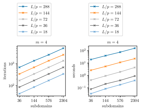
Figure 2: Weak scaling of CG with constant $m=4$ and $p\sim L$.

As expected from equations (44) and (45), it can be observed that the number of iterations and, consequently, the overall solve times scale like $I_{\text{Krylov}}\sim T_{\text{Krylov}}\sim L\sim p$. In particular, this shows that a Krylov method without adequate preconditioning will not result in a scalable solver.

We next turn to the proposed substructuring solver. The subdomain problems are factored using a Cholesky decomposition, provided by CHOLMOD [10].

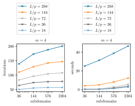
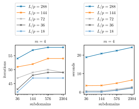
Figure 3: Weak scaling of the substructuring solver with constant $m=4$ and $p\sim L$. Top: No preconditioner, Cholesky solver in the operator. Bottom: Dirichlet preconditioner, Cholesky solvers in the operator and preconditioner.

We show the number of iterations of the projected CG method and overall solve times in the top row of Figure 3. The number of iterations appears to approach an asymptotic value that depends on $L/p$. Although the number of subdomains increases by a factor of $64$, the solve time increases at most by a factor of 1.85, which is in line with the predicted behavior in (46).

Next, we precondition the reduced system with the Dirichlet preconditioner described above. We also use a Cholesky factorization for the involved interior solves. Again, iterations and solve times are shown in the bottom row of Figure 3. The number of iterations varies between 42 and 58, and is asymptotically independent of the problem size and the number of subdomains. Similarly, the overall solve time is close to constant as the problem size is increased, but depends on the size of the subdomain problems. Clearly, use of the Dirichlet preconditioner leads to improvements in terms of iteration count and solve time compared to the unpreconditioned DD solver.

The memory cost of computing two Cholesky factorizations can be significant, in particular for large number of particle interactions $m$. It is therefore natural to attempt to reuse the factorization of the interior when solving the subdomain problem, or to replace the direct solvers with an iterative method. While using an inexact solve for the subdomains within the operator can easily lead to difficulties with regards to convergence towards the correct solution, we can replace the solve on the subdomain interior within the Dirichlet preconditioner with 5 iterations of CG and repeat the weak scaling experiment. The results in Figure 4 show a minor slow-down in the solve, but the overall scaling of the method is unaffected. We also show timings for $m=8$.

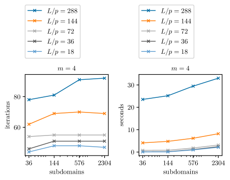
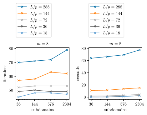
Figure 4: Weak scaling of the substructuring solver with constant $m$ (top: $m=4$, bottom: $m=8$) and $p\sim L$ and Cholesky solver in the operator and 5 iterations of CG in the Dirichlet preconditioner.

By selecting the problem with 2304 subdomains and $L/p=288$ for comparison between the four presented solver options, we observe that the CG solve took 157.16 seconds, while the domain decomposition solver takes 46.5s without preconditioner, 24.2s with Cholesky-Dirichlet preconditioner and 33s with CG-Dirichlet preconditioner. Based on the scaling estimates, speedups larger than 6.5x can be expected for bigger problems.

4.2 Weak scaling with constant $\delta$

In a second set of experiments, we fix the interaction length $\delta$ and vary the problem size $L$. This implies that the number of entries per matrix row will increase as $L$ increases. In order to keep the memory cost of the subdomain matrices $A_{i}$ under control, this means that the number of subdomains per direction needs to scale like $p\sim L^{2}$.

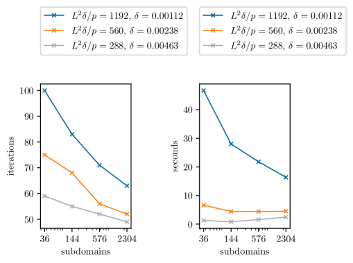
Figure 5: Weak scaling of the substructuring solver with constant $\delta$ and $p\sim L^{2}$.

Iteration counts and timings results for the DD method with CG-Dirichlet preconditioner are shown in Figure 5. Since $L/p\sim 1/L$, we observe decreasing iteration counts and solve times, as predicted by (46).

4.3 Strong scaling

In a final set of experiments, we explore the strong scaling properties of the substructuring solver. For a fixed choice of $L$, $m$ and $\delta=m/L$, we vary the number of subdomains per direction $p$. The resulting timings for $m=4$ and $m=8$ are shown in Figure 6. As observed, the strong scaling is almost optimal. For $m=4$, we see the strong scaling performance taper off as the number of subdomains is increased by 16. This can be explained by the fact that while computation is indeed divided by a factor of 16, communication is not and will start to dominate in the strong scaling limit. Naturally, for $m=8$ the amount of computation is higher, which explains the higher solve times compared to $m=4$, but also the better strong scaling behavior.

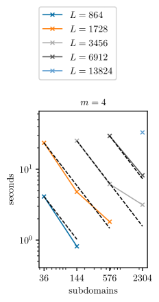
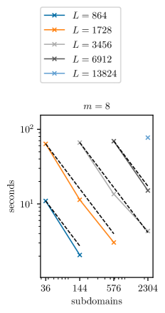
Figure 6: Strong scaling of the substructuring solver with constant $L$, $m$ and $\delta=m/L$. The dashed lines are the ideal strong scaling.

5 Conclusion

We have presented a domain decomposition technique for the efficient numerical solution of nonlocal diffusion problems. Our method, based on a meshfree discretization of the variational multi-domain formulation that was previously introduced in [9], solves the discretized problem in a FETI fashion and exploits effective preconditioning techniques introduced for local domain-decomposition problems.

Our rigorous numerical studies highlight the fact that the proposed approach outperforms commonly used parallel solvers. In fact, based on the scaling estimates derived in Section 4 and the corresponding numerical studies, we expect speedups (with respect to standard single-domain solvers) larger than 6.5x on problems of increasing size. Furthermore, our tests in Sections 4.1–4.3 show excellent scalability properties that confirm our theoretical estimates.

This work is the first rigorous numerical study in a two-dimensional multi-domain setting for nonlocal operators with finite horizon and, as such, it represents a fundamental step towards increasing the usability of nonlocal models in large scale simulations. It is possible to generalize the proposed technique to any linear nonlocal problem, including nonlocal elasticity, in a straightforward way just by adapting the discretization matrices associated with the sub-problems. Furthermore, due to the similarities between discretized nonlocal problems and systems resulting from long-stencil meshfree discretizations of PDEs, the impact of this work extends beyond nonlocal problems, as our algorithm can be applied without modifications to meshfree discretizations of PDEs.

References

• [1] Sandia National Labs High-Performance Computing. https://hpc.sandia.gov/HPC%20Production%20Clusters/index.html. Accessed: May 5, 2021.
• [2] B. Aksoylu and T. Mengesha. Results on nonlocal boundary value problems. Numerical functional analysis and optimization, 31(12):1301–1317, 2010.
• [3] B. Aksoylu and M. Parks. Variational theory and domain decomposition for nonlocal problems. Applied Mathematics and Computation, 217(14):6498–6515, 2011.
• [4] B. Aksoylu and Z. Unlu. Conditioning analysis of nonlocal integral operators in fractional sobolev spaces. SIAM Journal on Numerical Analysis, 52(2):653–677, 2014.
• [5] B. Alali and M. Gunzburger. Peridynamics and material interfaces. Journal of Elasticity, 120(2):225–248, 2015.
• [6] D. Benson, S. Wheatcraft, and M. Meerschaert. Application of a fractional advection-dispersion equation. Water Resources Research, 36(6):1403–1412, 2000.
• [7] M. Bessa, J. Foster, T. Belytschko, and W. Liu. A meshfree unification: Reproducing kernel peridynamics. Computational Mechanics, 53(6):1251–1264, 2014.
• [8] G. Capodaglio, M. D’Elia, P. Bochev, and M. Gunzburger. An energy-based coupling approach to nonlocal interface problems. Computers and Fluids, 207:104593, 2020.
• [9] G. Capodaglio, M. D’Elia, M. Gunzburger, P. Bochev, M. Klar, and C. Vollmann. A general framework for substructuring-based domain decomposition methods for models having nonlocal interactions. arXiv preprint arXiv:2008.11780, 2021.
• [10] Y. Chen, T. A. Davis, W. W. Hager, and S. Rajamanickam. Algorithm 887: Cholmod, supernodal sparse cholesky factorization and update/downdate. ACM Trans. Math. Softw., 35(3), Oct. 2008.
• [11] M. D’Elia, J. De los Reyes, and A. M. Trujillo. Bilevel parameter optimization for nonlocal image denoising models. arXiv1912.02347, 2019.
• [12] M. D’Elia, Q. Du, C. Glusa, X. Tian, and Z. Zhou. Numerical methods for nonlocal and fractional models. ACTA Numerica, 29, 2020.
• [13] M. D’Elia, Q. Du, M. Gunzburger, and R. Lehoucq. Nonlocal convection-diffusion problems on bounded domains and finite-range jump processes. Computational Methods in Applied Mathematics, 29:71–103, 2017.
• [14] M. D’Elia, M. Gulian, H. Olson, and G. E. Karniadakis. A unified theory of fractional, nonlocal, and weighted nonlocal vector calculus. arXiv:2005.07686, 2020.
• [15] M. D’Elia, X. Tian, and Y. Yu. A physically-consistent, flexible and efficient strategy to convert local boundary conditions into nonlocal volume constraints. SIAM Journal of Scientific Computing, 42(4):A1935–A1949, 2020.
• [16] Q. Du, M. Gunzburger, R. Lehoucq, and K. Zhou. Analysis and approximation of nonlocal diffusion problems with volume constraints. SIAM review, 54:667–696, 2012.
• [17] Q. Du, M. Gunzburger, R. Lehoucq, and K. Zhou. Analysis and approximation of nonlocal diffusion problems with volume constraints. SIAM Review, 54(4):667–696, 2012.
• [18] C. Farhat and F.-X. Roux. A method of finite element tearing and interconnecting and its parallel solution algorithm. International journal for numerical methods in engineering, 32(6):1205–1227, 1991.
• [19] M. Felsinger, M. Kassmann, and P. Voigt. The Dirichlet problem for nonlocal operators. Mathematische Zeitschrift, 279:779–809, 2015.
• [20] G. Gilboa and S. Osher. Nonlocal linear image regularization and supervised segmentation. Multiscale Model. Simul., 6:595–630, 2007.
• [21] Y. D. Ha and F. Bobaru. Characteristics of dynamic brittle fracture captured with peridynamics. Engineering Fracture Mechanics, 78(6):1156–1168, 2011.
• [22] T. Mathew. Domain decomposition methods for the numerical solution of partial differential equations, volume 61. Springer Science & Business Media, 2008.
• [23] M. Meerschaert and A. Sikorskii. Stochastic models for fractional calculus. Studies in mathematics, Gruyter, 2012.
• [24] T. Mengesha and Q. Du. Analysis of a scalar nonlocal peridynamic model with a sign changing kernel. Discrete & Continuous Dynamical Systems-B, 18(5):1415–1437, 2013.
• [25] M. Parks, D. Littlewood, J. Mitchell, and S. Silling. Peridigm users’ guide. Sandia National Laboratories, SANDIA REPORT(2012-7800):2012–7800, September 2012.
• [26] R. Schumer, D. Benson, M. Meerschaert, and B. Baeumer. Multiscaling fractional advection-dispersion equations and their solutions. Water Resources Research, 39(1):1022–1032, 2003.
• [27] S. A. Silling. Reformulation of elasticity theory for discontinuities and long-range forces. Journal of the Mechanics and Physics of Solids, 48(1):175–209, 2000.
• [28] X. Xu, M. D’Elia, and J. Foster. A machine-learning framework for peridynamic material models with physical constraints. Preprint arXiv:2101.01095, 2021.
• [29] X. Xu and J. T. Foster. Deriving peridynamic influence functions for one-dimensional elastic materials with periodic microstructure. arXiv preprint arXiv:2003.05520, 2020.
• [30] H. You, Y. Yu, S. Silling, and M. D’Elia. Data-driven learning of nonlocal models: from high-fidelity simulations to constitutive laws. arXiv:2012.04157, 2020.
• [31] H. You, Y. Yu, N. Trask, M. Gulian, and M. D’Elia. Data-driven learning of robust nonlocal physics from high-fidelity synthetic data. arXiv preprint arXiv:2005.10076, 2020.