An End-to-End Framework for Molecular Conformation Generation
via Bilevel Programming

Abstract

Predicting molecular conformations (or 3D structures) from molecular graphs is a fundamental problem in many applications. Most existing approaches are usually divided into two steps by first predicting the distances between atoms and then generating a 3D structure through optimizing a distance geometry problem. However, the distances predicted with such two-stage approaches may not be able to consistently preserve the geometry of local atomic neighborhoods, making the generated structures unsatisfying. In this paper, we propose an end-to-end solution for molecular conformation prediction called ConfVAE based on the conditional variational autoencoder framework. Specifically, the molecular graph is first encoded in a latent space, and then the 3D structures are generated by solving a principled bilevel optimization program. Extensive experiments on several benchmark data sets prove the effectiveness of our proposed approach over existing state-of-the-art approaches. Code is available at https://github.com/MinkaiXu/ConfVAE-ICML21.

1 Introduction

Recently we have witnessed much success of deep learning for molecule modeling in a variety of applications ranging from molecule property prediction (Gilmer et al., 2017) and molecule generation (You et al., 2018; Shi et al., 2020b) to retrosynthesis planning (Shi et al., 2020a). In these applications, molecules are generally represented as graphs with atoms as nodes and covalent chemical bonds as edges. Although this is empirically effective, in reality molecules are better represented as 3D structures (also known as conformations), where each atom is characterized by 3D Cartesian coordinates. Such 3D structures are also more intrinsic and informative, determining many chemical and biological properties such as chemical sensing and therapeutic interactions with proteins.

However, determining the 3D structures from experiments is challenging and costly. Effectively predicting valid and low-energy conformations has been a very important and active topic in computational chemistry. Traditional computational approaches are typically based on Markov chain Monte Carlo (MCMC) or molecular dynamics (MD) (De Vivo et al., 2016) to propose conformations combined with simulations to assign energies through cheap empirical potentials or expensive quantum chemical simulations (Ballard et al., 2015). Recently, there is growing interest in developing machine learning approaches (Mansimov et al., 2019; Simm & Hernández-Lobato, 2020; Xu et al., 2021) to model the conditional distribution $p({\bm{R}}|{\mathcal{G}})$ of stable conformations ${\bm{R}}$ given the molecular graph ${\mathcal{G}}$ by training on a collection of molecules with available stable conformations. Specifically, two recent works (Simm & Hernández-Lobato, 2020; Xu et al., 2021) propose to first predict the distances between atoms and then generate molecular conformations based on the predicted distances by solving a distance geometry problem (Liberti et al., 2014). Such approaches based on distance geometry effectively take into account the rotation and translation invariance of molecular conformations and have hence achieved very promising performance.

However, there is still a significant limitation for these two-stage approaches, which predict the distances and conformations separately: the predicted distances might not be able to properly preserve the 3D geometry of local atomic neighborhoods. Some invalid combinations of distances could be assigned a high likelihood according to the distance prediction model. The errors in these distances could be significantly exaggerated by the distance geometry program of the second stage, yielding unrealistic outlier samples of 3D structures. This is not surprising as the distance prediction model is trained by maximizing the factorized likelihood of distances while our end goal is to predict valid and stable conformations. We propose to effectively address this issue with an end-to-end solution which directly predicts the conformation given the molecular graph. Indeed, in a related problem of predicting 3D structures of proteins (a.k.a. protein structure prediction) based on amino-acid sequences, the recent huge success of the AlphaFold2 algorithm shows the importance and effectiveness of developing an end-to-end solution compared to the previous AlphaFold algorithm (though exact details of AlphaFold2 algorithm are still lacking) (Senior et al., 2020a; Jumper et al., 2020).

In this paper, we propose such an end-to-end solution called ConfVAE for molecular conformation generation, based on bilevel programming. To model the rotational and translational invariance of conformations, we still take the pairwise distances among atoms as intermediate variables. However, instead of learning to predict distances by minimizing errors in the space of distance, we formulate the whole problem as bilevel programming (Franceschi et al., 2018), with the distance prediction problem and the distance geometry problem for conformation generation being simultaneously optimized. The whole framework is built on the conditional variational autoencoder (VAE) framework (Kingma & Welling, 2013), in which the molecular graph is first encoded into the VAE latent space, and the conformations are generated based on the latent variable and molecular graph. During training, we iteratively sample a set of distances from the distance prediction model, generate the 3D structures by minimizing an inner objective (defined by the distance geometry problem), and then update the distance prediction model by optimizing the outer objective, i.e., the likelihood directly defined on the conformations.

To the best of our knowledge, ConfVAE is the first method for molecular conformation generation which can be trained in an end-to-end fashion and at the same time keep the property of rotational and translational invariance. Extensive experiments demonstrate the superior performance of the proposed method over existing state-of-the-art approaches on several widely used benchmarks including conformation generation and distance distribution modeling. We also verify that the end-to-end objective is of vital importance for generating realistic and meaningful conformations.

2 Background

2.1 Problem Definition

Notations. Following existing work (Simm & Hernández-Lobato, 2020; Xu et al., 2021), each molecule is represented as an attributed atom-bond graph ${\mathcal{G}}=\langle{\mathcal{V}},{\mathcal{E}}\rangle$, where ${\mathcal{V}}$ is the set of vertices representing atoms and ${\mathcal{E}}$ is the set of edges representing inter-atomic bonds. Each node $v$ in ${\mathcal{V}}$ describes the chosen atomic features such as element type. Each edge $e_{uv}$ in ${\mathcal{E}}$ describes the corresponding chemical bond connecting $u$ and $v$, and is labeled with its bond type. Since the distances of bonds existing in the molecular graph are not sufficient to determine an unique conformation (e.g.due to so-called internal rotations around the axis of the bond), we adopt the common pre-processing methodology in existing works (Simm & Hernández-Lobato, 2020; Xu et al., 2021) to expand the graphs by incorporating auxiliary edges, which force multi-hop distance constraint eliminating some ambiguities in the 3D conformation, as elaborated in Appendix A.

For the geometry ${\bm{R}}$, each atom in ${\mathcal{V}}$ is represented by a 3D coordinate vector ${\bm{r}}\in{\mathbb{R}}^{3}$, and the full set of positions $\{{\bm{r}}_{v}\}_{v\in{\mathcal{V}}}$ is represented by the matrix ${\bm{R}}\in{\mathbb{R}}^{|{\mathcal{V}}|\times 3}$. Let $d_{uv}$ denote the Euclidean distance $\|{\bm{r}}_{u}-{\bm{r}}_{v}\|_{2}$ between the $u^{th}$ and $v^{th}$ atom, then all the distances between connected nodes $\{d_{uv}\}_{e_{uv}\in{\mathcal{E}}}$ can be summarized as a vector ${\bm{d}}\in{\mathbb{R}}^{|{\mathcal{E}}|}$.

Problem Definition. The problem of molecular conformation generation is a conditional generation process, where the goal is to model the conditional distribution of molecular conformations ${\bm{R}}$ given the graph ${\mathcal{G}}$, i.e., $p({\bm{R}}|{\mathcal{G}})$.

2.2 Bilevel Optimization

Bilevel programs are defined as optimization problems where a set of variables involved in the (outer) objective function are obtained by solving another (inner) optimization problem (Colson et al., 2007). Formally, given the outer objective function $F$ and the inner objective $H$, and the corresponding outer and inner variables $\theta$ and $w$, a bilevel program can be formulated by

$$\min_{{\theta}}F(w_{\theta})\ \ \text{such that}\ \ w_{\theta}\in\arg\min_{w}H(w,\theta).$$ (1)

Bilevel programs have shown effectiveness in a variety of situations such as hyperparameter optimization, adversarial and multi-task learning, as well as meta-learning (Maclaurin et al., 2015; Bengio, 2000; Bennett et al., 2006; Flamary et al., 2014; Muñoz-González et al., 2017; Franceschi et al., 2018).

Typically solving equation 1 is intractable since the solution sets of $w_{\theta}$ may not be available in closed form (Bengio, 2000). A common approach is to replace the exact minimizer of the inner object $H$ with an approximation solution, which can be obtained through an iterative optimization dynamics $\Phi$ such as stochastic gradient descent (SGD) (Domke, 2012; Maclaurin et al., 2015; Franceschi et al., 2017). Starting from the initial parameter $w_{0}$, we can get the approximate solution $w_{\theta,T}$ by running $T$ iterations of the inner optimization dynamics $\Phi$, i.e., $w_{\theta,T}=\Phi(w_{\theta,T-1},\theta)=\Phi(\Phi(w_{\theta,T-2},\theta),\theta)$, and so on. In the general case where $\theta$ and $w$ are real-valued and the objectives and optimization dynamics is smooth, the gradient of the object $F(w_{\theta,T})$ w.r.t. $\theta$, named hypergradient $\nabla_{\theta}F(w_{\theta,T})$, can be computed by:

$$\nabla_{\theta}F(w_{\theta,T})=\partial_{w}F(w_{\theta,T})\nabla_{\theta}w_{\theta,T}$$ (2)

where $\partial$ denotes the partial derivative to compute the Jacobian on immediate variables while $\nabla$ denotes a total derivative taking into account the recursive calls to $F$. The above gradient can be efficiently calculated by unrolling the optimization dynamics with back-propagation, i.e., reverse-mode automatic differentiation (Griewank & Walther, 2008), where we repeatedly substitute $w_{\Phi,t}=\Phi(w_{\theta,t-1},\theta)$ and apply the chain rule.

3 Implicit Distance Geometry

In this section we elaborate on the proposed end-to-end framework. We first present a high-level description of our bilevel formulation in Sec. 3.1. Then we present the model schematic and training objectives in Sec. 3.2. Finally we show how to learn the model via hypergradient descent in Sec. 3.3 and how to draw samples in Sec. 3.4.

3.1 Overview

Since a molecule can have multiple stable conformations, we model the distribution of conformations ${\bm{R}}$ conditioning on molecular graph ${\mathcal{G}}$ (i.e. $p({\bm{R}}|{\mathcal{G}})$) with a conditional variational autoencoder (CVAE) (Kingma & Welling, 2013), in which a latent variable $z$ is introduced to model the uncertainty in molecule conformation generation. The CVAE model includes a prior distribution of latent variable $p_{\psi}(z|{\mathcal{G}})$ and a decoder $p_{\theta}({\bm{R}}|z,{\mathcal{G}})$ to capture the conditional distribution of ${\bm{R}}$ given $z$. During training, we also involve an additional inference model (encoder) $q_{\phi}(z|{\bm{R}},{\mathcal{G}})$. The encoder and decoder are jointly trained to maximize the evidence lower bound (ELBO) of the data log-likelihood:

$$\log P({\bm{R}}|{\mathcal{G}})\geq \mathbb{E}_{z\sim q_{\phi}(z|{\bm{R}},\mathcal{G})}\left[\log p_{\theta}({\bm{R}}|z,\mathcal{G})\right]$$ (3)

$$-D_{\mathrm{KL}}\left[q_{\phi}(z|{\bm{R}},\mathcal{G})\|p_{\psi}(z|\mathcal{G})\right]$$

$$\triangleq {\mathcal{L}}_{ELBO}(\theta,\phi,\psi),$$

The ELBO can be interpreted as the sum of the negative reconstruction error ${\mathcal{L}}_{recon}$ (the first term) and a latent space prior regularizer ${\mathcal{L}}_{prior}$ (the second term). In practice, $q_{\phi}(z|{\bm{R}},\mathcal{G})$ and $p_{\psi}(z|\mathcal{G})$ are all modeled as diagonal Gaussians $N(z|\mu_{\phi}({\bm{R}},\mathcal{G}),\sigma_{\phi}({\bm{R}},\mathcal{G}))$ and $N(z|\mu_{\psi}({\mathcal{G}}),\sigma_{\psi}({\mathcal{G}}))$, whose mean and standard deviation are predicted by graph neural networks. To efficiently optimize the ELBO during training, sampling from $q_{\phi}(z|{\bm{R}},\mathcal{G})$ is done by reparametrizing $z$ as $z_{\phi}=\mu_{\phi}({\bm{R}},\mathcal{G})+\sigma_{\phi}({\bm{R}},\mathcal{G})\cdot\epsilon$, where $\epsilon\sim{\mathcal{N}}({\bm{0}},{\bm{I}})$.

With similar encoder and prior models, the key differences among different methods lie in the architecture and learning method of the decoder (generator) model $p_{\theta}({\bm{R}}|z,\mathcal{G})$, i.e., how to parameterize the decoder and train it with respect to the reconstruction loss ${\mathcal{L}}_{recon}$. Let $D_{\theta}(z,{\mathcal{G}})$ denote the decoder function taking prior $z$ and graph ${\mathcal{G}}$ to obtain a distance vector, we now elaborate how we formulate the optimization problem of the decoder as a bilevel program:

Inner objective: Directly generating conformations as Cartesian coordinates heavily depends on the arbitrary rotation and translation. Therefore, previous effective approaches (Simm & Hernández-Lobato, 2020; Xu et al., 2021) instead make the decoder generate inter-atomic distances ${\bm{d}}$, i.e., ${\bm{d}}_{\theta,\phi}=D_{\theta}(z_{\phi},{\mathcal{G}})$. The distances ${\bm{d}}$ are taken as intermediate variables to generate conformations, which are invariant to rotation and translation. To generate a conformation ${\bm{R}}$, one needs to first generate the set of distances ${\bm{d}}$, and then post-process ${\bm{d}}$ to obtain the 3D positions ${\bm{R}}$, by solving a distance geometry optimization problem:

$${\bm{R}}_{\theta,\phi} =\arg\min_{\bm{R}}H({\bm{R}},D_{\theta}(z_{\phi},{\mathcal{G}}))$$ (4)

$$=\arg\min_{\bm{R}}H({\bm{R}},{\bm{d}}_{\theta,\phi})$$

$$=\arg\min_{\bm{R}}\Big{\{}\sum_{e_{uv}\in{\mathcal{E}}}\big{(}\|{\bm{r}}_{u}-{\bm{r}}_{v}\|_{2}-d_{uv}\big{)}^{2}\Big{\}},$$

which we take as the inner loop objective.

Outer objective: Ultimately, we are interested in directly minimizing the generalization error on 3D structures to make the generated conformation consistent with the ground-truth up to rotation and translation. The post-alignment Root-Mean-Square Deviation (RMSD) is a widely used metric for this purpose. To calculate this metric, another conformation $\hat{{\bm{R}}}$ is first obtained by an alignment function $\hat{{\bm{R}}}=A({\bm{R}},{\bm{R}}^{*})$, which rotates and translates the reference conformation ${\bm{R}}^{*}$ to have the smallest distance to the generated one ${\bm{R}}$ according to the RMSD metric:

$$\operatorname{RMSD}({\bm{R}},\hat{{\bm{R}}})=\Big{(}\frac{1}{n}\sum_{i=1}^{n}\|{\bm{R}}_{i}-\hat{{\bm{R}}_{i}}\|^{2}\Big{)}^{\frac{1}{2}}.$$ (5)

where $n$ is the number of atoms. Then the reconstruction objective ${\mathcal{L}}_{recon}$ can be written as:

$$F({\bm{R}}_{\theta,\phi}) =\log p_{\theta}({\bm{R}}|z,\mathcal{G})$$ (6)

$$=-\sum_{i=1}^{n}\sum_{j=1}^{3}\left({\bm{R}}_{ij}-A({\bm{R}},{\bm{R}}^{*})_{ij}\right)^{2},$$

which is the outer loop objective for computing the reconstruction loss and maximize the log-likelihood.

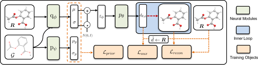
Figure 1: The overall framework of ConfVAE. At training time, given the graph ${\mathcal{G}}$ and conformation ${\bm{R}}$, we: 1) compute the distributions of $q_{\phi}(z|{\mathcal{G}},{\bm{R}})$ and $p_{\psi}(z|{\mathcal{G}})$, and calculate ${\mathcal{L}}_{prior}$; 2) sample $z$ from $q_{\phi}$ by reparameterization, and feed it into the decoder (generator) $p_{\theta}$ to generate inter-atomic distances ${\bm{d}}$, after which we can obtain an auxiliary objective ${\mathcal{L}}_{aux}$ from the true distances $\hat{{\bm{d}}}$ derived from ${\bm{R}}$; 3) run the inner loop (distance geometry) to recover the 3D structure from ${\bm{d}}$, and compute the reconstruction RMSD loss ${\mathcal{L}}_{recon}$. The model is trained end-to-end by optimizing the sum of three object components ${\mathcal{L}}_{prior}$, ${\mathcal{L}}_{aux}$ and ${\mathcal{L}}_{recon}$.

Bilevel program: Now we can consider equation 4 and equation 6 as the inner and outer objectives of a bilevel programming problem. In this formulation, the outer objective aims to model the true conditional distribution $p({\bm{R}}|{\mathcal{G}})$, and the inner objective solves for the conformation given a set of predicted distances. By taking the expectation over latent variable $z$, the resulting bilevel program for calculating the reconstruction term ${\mathcal{L}}_{recon}$in equation 3 can be written as:

$$\max_{\theta,\phi}\mathbb{E}_{z\sim q_{\phi}(z|{\bm{R}},\mathcal{G})}\left[F({\bm{R}}_{\theta,\phi},\theta)\right]$$ (7)

such $$\text{that }{\bm{R}}_{\theta,\phi}=\arg\min_{\bm{R}}H({\bm{R}},D_{\theta}(z_{\phi},{\mathcal{G}})).$$ (8)

The derived bilevel problem is still challenging because: 1) the solution of conformation structure in the inner problem is not available in closed form; 2) computing this expectation exactly over the continuous latent space is intractable. Thus, in practice we compute an empirical estimation of the output with a variational inference model and the reparametrization trick. We elaborate on how we address these issues in the following parts.

3.2 Generative Model

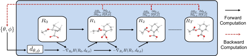
Figure 2: Schematic illustration of the forward and backward computational graph through the inner loop (distance geometry optimization). We repeatedly update ${\bm{R}}$ with the gradient $\nabla_{\bm{R}}H$ during the forward computation, and accumulate hypergradients $\nabla_{\theta,\phi}{\bm{R}}$ to update parameters $\theta$ and $\phi$ from backward computation.

We now have the tools needed to define our conditional generative model of molecular conformation. The cornerstone of all modules (encoder, prior and decoder) is message-passing neural networks (MPNNs) (Gilmer et al., 2017), which is a variant of graph neural networks that achieves state-of-the-art performance in representation learning for molecules (Scarselli et al., 2008; Bruna et al., 2013; Duvenaud et al., 2015; Kipf & Welling, 2016; Kearnes et al., 2016; Schütt et al., 2017). The MPNN directly operates on the graph representation ${\mathcal{G}}$ and is invariant to graph isomorphism. In each convolutional (message passing) layer, atomic embeddings are updated by aggregating the information from neighboring nodes.

For the encoder $q_{\phi}(z|{\bm{R}},{\mathcal{G}})$ and prior $p_{\psi}(z|{\mathcal{G}})$, we use the same MPNN architecture as Mansimov et al. (2019); Simm & Hernández-Lobato (2020). Since bilevel optimization has a relatively high memory cost, we use an ordinary differential equation (ODE)-based continuous normalizing flow (Chen et al., 2018) (CNF) for the decoder $p_{\theta}({\bm{R}}|z,{\mathcal{G}})$, which has constant memory cost. We describe the details of our decoder model below.

Decoder Architecture. As illustrated in Sec. 3.1, our decoder is composed of two cascaded levels: a distance prediction model $D_{\theta}(z,{\mathcal{G}})$ that decodes $z$ back into a set of distances ${\bm{d}}$, and a differentiable distance geometry procedure to recover geometry ${\bm{R}}$ from distances ${\bm{d}}$. The model $D_{\theta}(z,{\mathcal{G}})$ is implemented as a conditional extension of the CNF which transforms noise variables ${\bm{d}}(t_{0})$ (also the initial distances in the CNF ODE trajectory) sampled from the prior distribution ${\mathcal{N}}({\bm{0}},{\bm{I}})$ to final distances ${\bm{d}}={\bm{d}}(t_{1})$. The transformation is conditioned on the latent variable $z$ as well as the graph ${\mathcal{G}}$:

$${\bm{d}} =D_{\theta}(z,{\mathcal{G}})$$ (9)

$$={\bm{d}}(t_{0})+\int_{t_{0}}^{t_{1}}g_{\theta}({\bm{d}}(t),t,{\mathcal{G}},z){\operatorname{d}}t,$$

where $g_{\theta}$ is an MPNN that defines the continuous-time dynamics of the flow $D_{\theta}$ conditioned on $z$ and ${\mathcal{G}}$. Note that, given the true distances ${\bm{d}}(t_{1})={\bm{d}}$, ${\bm{d}}(t_{0})$ can also be easily computed by reversing the continuous dynamics $D_{\theta}$: $D_{\theta}^{-1}(z,{\mathcal{G}})={\bm{d}}(t_{1})+\int_{t_{1}}^{t_{0}}g_{\theta}({\bm{d}}(t),t,z,{\mathcal{G}}){\operatorname{d}}t$. And thus the exact conditional log-likelihood of distances given ${\mathcal{G}}$ can be computed by:

$$\mathcal{L}_{aux} =\log{p_{\theta}({\bm{d}}|z,{\mathcal{G}})}$$ (10)

$$=\log{p({\bm{d}}(t_{0}))}-\int_{t_{0}}^{t_{1}}\operatorname{Tr}\left(\frac{\partial g_{\theta}}{\partial{\bm{d}}(t)}\right){\operatorname{d}}t.$$

An ODE solver can then be applied to estimate the gradients on parameters for optimization. In practice, ${\mathcal{L}}_{aux}$ can be taken as an auxiliary objective defined on distances to supervise the training. In summary, the training objective can be interpreted as the sum of three parts:

$${\mathcal{L}}(\theta,\phi,\psi)={\mathcal{L}}_{recon}+\lambda{\mathcal{L}}_{prior}+\alpha{\mathcal{L}}_{aux},$$ (11)

where $\lambda$ and $\alpha$ are hyperparameters to reweight each component. The overall framework is illustrated in Fig. 1.

3.3 End-to-end Learning via Hypergradient Descent

We now discuss how to optimize the bilevel problem defined by equation 8 and equation 7 through a practical algorithm. The inner problem in equation 8 is a classic distance geometry problem about how to infer 3D coordinates from pairwise distances (Anand & Huang, 2018; Simm & Hernández-Lobato, 2020; Xu et al., 2021). Others have used a semi-definite program (SDP) to infer protein structure from nuclear magnetic resonance data (Alipanahi et al., 2013), or an Alternating Direction Method of Multipliers (ADMM) algorithm to fold the protein into the 3D Cartesian coordinates (Anand & Huang, 2018). In this initial work we choose gradient descent (GD), with tractable learning dynamics $\Phi$, to approximately solve for the geometry:

$${\bm{R}}_{{\theta,\phi},t+1}=\Phi({\bm{R}}_{{\theta,\phi},t},{\bm{d}}_{\theta,\phi})={\bm{R}}_{{\theta,\phi},t}-\eta\nabla H({\bm{R}}_{{\theta,\phi},t},{\bm{d}}_{\theta,\phi}),$$ (12)

where $\eta$ is the learning rate and ${\bm{d}}_{\theta,\phi}$ is the distance set generated from the distance prediction model. Under appropriate assumptions and for a number of updates $t\rightarrow\infty$, GD can converge to a proper geometry ${\bm{R}}_{\theta,\phi}$ that depends on the predicted pairwise distances (Bottou, 2010).

Now we consider how to calculate the hypergradient $\nabla_{\theta,\phi}\mathbb{E}_{z\sim q_{\phi}(z|{\bm{R}},\mathcal{G})}\left[F({\bm{R}}_{\theta,\phi})\right]$ from the outer loop reconstruction objective (equation 7) to train the model. Let ${\bm{R}}_{{\theta,\phi},T}$ denote the conformation generated by approximately solving for the distance geometry with $T$ steps gradient descent. Now we can write the hypergradient as:

$$\nabla_{\theta,\phi}\mathbb{E} {}_{z\sim q_{\phi}(z|{\bm{R}},\mathcal{G})}\left[F({\bm{R}}_{{\theta,\phi},T})\right]$$ (13)

$$=\mathbb{E}_{z\sim q_{\phi}(z|{\bm{R}},\mathcal{G})}\partial_{{\bm{R}}}\left[F({\bm{R}}_{{\theta,\phi},T})\right]\nabla_{\theta,\phi}{\bm{R}}_{{\theta,\phi},T},$$

where the gradient $\nabla_{\theta,\phi}{\bm{R}}_{\theta,\phi,T}$ can be computed by fully unrolling the dynamics of inner loop from $R_{T}$ to $R_{0}$. Specifically, in the forward computation, successive geometries ${\bm{R}}_{0,\cdots,T}$ resulting from the optimization dynamics are cached. In the backward call, the cached geometries are used to compute gradients in a series of Vector-Jacobian Products (VJPs). During the reverse computation, the gradient starting from the $\partial_{{\bm{R}}_{T}}F$ can be propagated to the intermediate geometries $R_{t}$ through $\nabla_{{\bm{R}}_{t}}{\bm{R}}_{t+1}$:

$$\nabla_{{\bm{R}}_{t}}{\bm{R}}_{t+1} =\nabla_{{\bm{R}}_{t}}\big{(}{\bm{R}}_{t}-\eta\nabla_{{\bm{R}}_{t}}H({\bm{d}}_{\phi,\theta},{\bm{R}}_{t})\big{)}$$ (14)

$$=1-\eta\nabla^{2}_{{\bm{R}}_{t}}H({\bm{d}}_{\phi,\theta},{\bm{R}}_{t})$$

where $\nabla^{2}_{{\bm{R}}_{t}}$ denotes the Hessian w.r.t. ${{\bm{R}}_{t}}$. With iteratively computed derivatives $\nabla_{{\bm{R}}_{t}}{\bm{R}}_{T}$, the adjoints on ${\bm{d}}_{\phi,\theta}$ can be computed in forms of VJPs and further backpropagated to the parameters of encoder $q_{\phi}$ and decoder $p_{\theta}$. Formally, $\nabla_{\bm{d}}{\bm{R}}_{T}$ is computed by:

$$\nabla_{{\bm{d}}_{\theta,\psi}}{\bm{R}}_{T} =\sum_{t=T-1}^{0}[\nabla_{{\bm{R}}_{t+1}}{\bm{R}}_{T}]\nabla_{{\bm{d}}}{\bm{R}}_{t+1}$$ (15)

$$=-\eta\sum_{t=T-1}^{0}[\nabla_{{\bm{R}}_{t+1}}{\bm{R}}_{T}]\nabla_{{\bm{d}}}\big{(}\nabla_{{\bm{R}}_{t}}H({\bm{d}}_{\phi,\theta},{\bm{R}}_{t})\big{)},$$

where $\nabla_{{\bm{R}}_{t+1}}{\bm{R}}_{T}$ can be substituted by equation 14. The computation can be done efficiently with reverse-mode automatic differentiation software such as PyTorch (Paszke et al., 2019). A schematic illustration of the forward and backward computational graph through distance geometry is presented in Fig. 2. We provide a detailed algorithm of the training procedure in Appendix. B.

3.4 Sampling

Given the graph ${\mathcal{G}}$, to generate a conformation ${\bm{R}}$, we first draw the latent variable $\tilde{z}$ from the prior distribution $p_{\psi}(z|{\mathcal{G}})$. Then we sample the random initial distances ${\bm{d}}(t_{0})$ from a Gaussian distribution, then pass $\tilde{{\bm{d}}}(t_{0})$ through the invertible Neural ODE $G_{\theta}$ conditioned on $\tilde{z}$ and ${\mathcal{G}}$ to obtain the distance set $\tilde{{\bm{d}}}=G_{\theta}(\tilde{{\bm{d}}}(t_{0});z,{\mathcal{G}})$. Then we produce the conformation ${\bm{R}}$ by solving the distance geometry optimization problem $\arg\min_{\bm{R}}H({\bm{R}},{\bm{d}}_{\theta,\phi})$ as defined in equation 4.

Table 1: Comparison of different methods on the conformation generation task. Top $5$ rows: deep generative models for molecular conformation generation. Bottom $6$ rows: different methods with an additional rule-based force field to further optimize the generated structures. We report the COV and MAT scores, where Mean and Median are calculated over different molecular graphs in the test set of GEOM. In practice, the size of the generated set is sampled as two times of the reference set following Xu et al. (2021).

[b] Dataset GEOM-QM9 GEOM-Drugs Metric COV^∗ (%) MAT (Å) COV^∗ (%) MAT (Å) Mean Median Mean Median Mean Median Mean Median CVGAE 8.52 5.62 0.7810 0.7811 0.00 0.00 2.5225 2.4680 GraphDG 55.09 56.47 0.4649 0.4298 7.76 0.00 1.9840 2.0108 CGCF 69.60 70.64 0.3915 0.3986 49.92 41.07 1.2698 1.3064 ConfVAE- 75.57 80.76 0.3873 0.3850 51.24 46.36 1.2487 1.2609 ConfVAE 77.98 82.82 0.3778 0.3770 52.59 56.41 1.2330 1.2270 RDKit 79.94 87.20 0.3238 0.3195 65.43 70.00 1.0962 1.0877 CVGAE + FF 63.10 60.95 0.3939 0.4297 83.08 95.21 0.9829 0.9177 GraphDG + FF 70.67 70.82 0.4168 0.3609 84.68 93.94 0.9129 0.9090 CGCF + FF 73.52 72.75 0.3131 0.3251 92.28 98.15 0.7740 0.7338 ConfVAE- + FF 77.95 79.14 0.2851 0.2817 91.48 99.21 0.7743 0.7436 ConfVAE + FF 81.46 83.80 0.2702 0.2709 91.88 100.00 0.7634 0.7312

• For COV, the threshold $\delta$ is set as $0.5\mathrm{\AA}$ for QM9 and $1.25\mathrm{\AA}$ for Drugs following Xu et al. (2021).

4 Experiments

4.1 Experiment Setup

Evaluation Tasks. Following previous work on conformation generation (Mansimov et al., 2019; Simm & Hernández-Lobato, 2020; Xu et al., 2021), we conduct extensive experiments by comparing our method with the state-of-the-art baseline models on several standard tasks. Conformation Generation is formulated by Xu et al. (2021), who concentrate on the models’ capacity to generate realistic and diverse molecular conformations. Distance distribution modeling is first proposed by Simm & Hernández-Lobato (2020), who evaluate whether the methods can model the underlying distribution of distances.

Baselines. We compared our proposed model with the following state-of-the-art conformation generation methods. CVGAE (Mansimov et al., 2019) is a conditional VAE-based model, which applied a few layers of graph neural networks to learn the atom representation from the molecular graph, and then directly predicts the 3D coordinates. GraphDG (Simm & Hernández-Lobato, 2020) also employs the conditional VAE framework. Instead of directly generating the conformations in 3D coordinates, they instead learn the distribution over distances. Then the distances are converted into conformations with a distance geometry algorithm. CGCF (Xu et al., 2021), another two-stage method, uses continuous normalizing flows to predict the atomic pairwise distances. Following the baselines, we also compare our model with RDKit (Riniker & Landrum, 2015), a classical distance geometry approach built upon an extensive calculation collection of edge lengths by computational chemistry.

Featurization and Implementation. The MPNNs used for the encoder, prior and decoder are all implemented as Graph Isomorphism Networks (Xu et al., 2018; Hu et al., 2019). For the input features of the graph representation, we only derive the atom and bond types from molecular graphs. As a default setup, the MPNNs are all implemented with $3$ layers, and the hidden embedding dimension is set as $256$. For the training of ConfVAE, we train the model on a single Tesla V100 GPU with a batch size of $128$ and a learning rate of $0.001$ until convergence, with Adam (Kingma & Welling, 2013) as the optimizer.

4.2 Conformation Generation

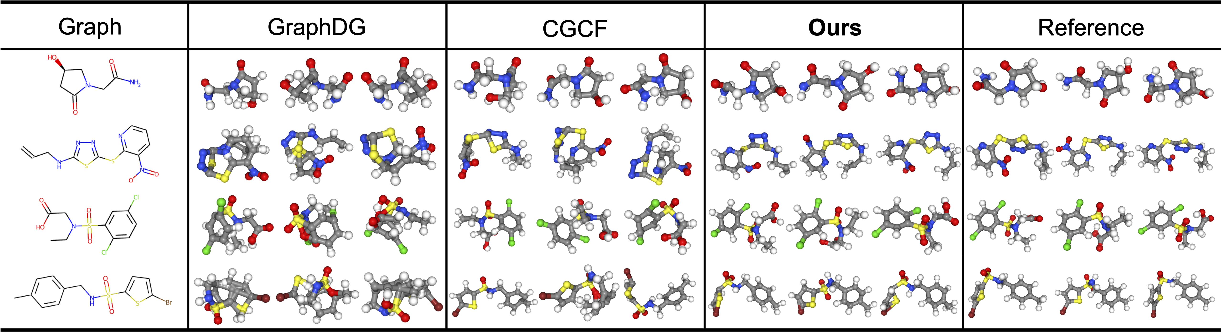
Figure 3: Visualization of generated conformations from state-of-the-art baselines, our method and the reference set, where four molecular graphs are randomly taken from the test set of GEOM-Drugs. C, O, H, S and Cl are colored gray, red, white, yellow and green respectively.

Datasets. Following Xu et al. (2021), we use the recent proposed GEOM-Drugs and GEOM-Drugs  (Axelrod & Gomez-Bombarelli, 2020) datasets for the conformation generation task. The Geometric Ensemble Of Molecules (GEOM) dataset contains millions of high-quality stable conformations, which is suitable for the conformation generation task. The GEOM-Drugs dataset consists of generally medium-sized organic compounds, containing an average of 44.2 atoms. We follow the setting from Xu et al. (2021) to randomly take 50000 conformation-molecule pairs as the training set, and another 9161 conformations (covering 100 molecular graphs) as the test split. By contrast, GEOM-QM9 is a much smaller dataset limited to small molecules with 9 heavy atoms. Similarly, we randomly draw 50000 conformation-molecule pairs to constitute the training set, and another 17813 conformations covering 150 molecular graphs as the test set.

Evaluation metrics. In this task we hope the generated samples to be of both high quality and diversity. We follow previous work (Hawkins, 2017; Mansimov et al., 2019; Xu et al., 2021) to calculate the RMSD of the heavy atoms between generated samples and reference ones. Given the generated conformation ${\bm{R}}$ and the reference ${\bm{R}}^{*}$, we take the same alignment function $A({\bm{R}},{\bm{R}}^{*})$ defined in equation 5 to obtain the aligned conformation $\hat{{\bm{R}}}$, and then calculate the evaluation metric by $\operatorname{RMSD}({\bm{R}},\hat{{\bm{R}}})=\Big{(}\frac{1}{n}\sum_{i=1}^{n}\|{\bm{R}}_{i}-\hat{{\bm{R}}_{i}}\|^{2}\Big{)}^{\frac{1}{2}}$, where $n$ is the number of heavy atoms. Built upon the RMSD metric, Xu et al. (2021) defined Coverage (COV) and Matching (MAT) scores to measure the diversity and quality respectively. COV counts the fraction of conformations in the reference set that are covered by at least one conformation in the generated set:

$$\operatorname{COV}( {\mathbb{S}}_{g}({\mathcal{G}}),{\mathbb{S}}_{r}({\mathcal{G}}))=$$ (16)

$$\frac{1}{|{\mathbb{S}}_{r}|}\Big{|}\Big{\{}{\bm{R}}\in{\mathbb{S}}_{r}\big{|}\operatorname{RMSD}({\bm{R}},{\bm{R}}^{\prime})<\delta,\exists{\bm{R}}^{\prime}\in{\mathbb{S}}_{g}\Big{\}}\Big{|}.$$

where ${\mathbb{S}}_{g}({\mathcal{G}})$ and ${\mathbb{S}}_{r}({\mathcal{G}})$ denote the generated and the reference conformations set respectively. Typically, a higher COV score indicates a better diversity performance to cover the complex true distribution.

While COV is able to detect mode-collapse, there is no guarantee for the quality of generated samples. Thus, the MAT score is defined as a complement metric that concentrates on the quality (Xu et al., 2021):

$$\operatorname{MAT}({\mathbb{S}}_{g}({\mathcal{G}}),{\mathbb{S}}_{r}({\mathcal{G}}))=\frac{1}{|{\mathbb{S}}_{r}|}\sum_{{\bm{R}}^{\prime}\in{\mathbb{S}}_{r}}\min_{{\bm{R}}\in{\mathbb{S}}_{g}}\operatorname{RMSD}({\bm{R}},{\bm{R}}^{\prime}).$$ (17)

Generally, more realistic generated samples lead to a lower MAT score.

Results. We calculate the COV and MAT evaluations on both GEOM-QM9 and GEOM-Drugs datasets for all baselines, and summarize the results in Tab. 1. We visualize several representative examples in Fig. 3. Our ConfVAE outperforms all existing strong baselines with an obvious margin (top $5$ rows). By incorporating an end-to-end training objective via bilevel optimization, we consistently achieved a better result on all four metrics. By contrast, current state-of-the-art models GraphDG and CGCF suffer much worse performance due to the two-stage generation process, where the extra error caused by the distance geometry cannot be taken into account during training. CVGAE enjoys the same training and testing objective, but still shows inferior performance since it fails to keep the vital translation and rotation invariant property.

Similar to previous work (Mansimov et al., 2019; Xu et al., 2021), we also further test all models by incorporating a rule-based empirical force field (Halgren, 1996b) and compare the performance with the classic RDKit toolkit. Specifically, we first generate the conformations with the generative models as initial structures, and then utilize the force field to further optimize the generated structures. The additional results are reported in Tab. 1 (bottom $6$ rows). As shown in the table, ConfVAE still achieves the best results among all generative models. More importantly, our method outperforms RDKit on $7$ out of $8$ evaluations and achieves competitive results on the other one, making our method the first generative model that already practically useful for real-world applications.

Ablation Study. So far we have demonstrated the superior performance of the proposed method. However, because we adopt a slightly different architecture, it remains unclear where the effectiveness comes from. In this part, we carefully conduct an ablation study by removing the bilevel component defined in equation 7 during training, i.e., remove ${\mathcal{L}}_{recon}$ and learn the model with only ${\mathcal{L}}_{aux}$ and ${\mathcal{L}}_{prior}$. We denote this variant of ConfVAE as ConfVAE-. and summarize the additional results in Tab. 1.

As shown in the table, removing the bilevel component hurts performance. These results verify that only learning from distances will introduce an extra bias for the generated conformations, and our end-to-end method for directly learning on the 3D structure helps to overcome this issue. Another observation is that as a combination of flow-based and VAE-based model, ConfVAE- still achieves significantly better results than the Flow-based CGCF and VAE-based GraphDG, with exactly the same training and sampling process. This result indicates that incorporating both global ($z$) and local ${\bm{d}}(t_{0})$ latent variables will contribute to the generated conformations, which can help to capture both the global and local geometric structure and atomic interactions.

Table 2: Comparison of different models on the distance distribution modeling task. We compare the marginals ($p(d_{uv}|{\mathcal{G}})$), pairs ($p(d_{uv},d_{ij}|{\mathcal{G}})$) and joint distribution ($p({\bm{d}}|{\mathcal{G}})$) of edges connecting C and O atoms. We report the Median and Mean of the MMD metric. Molecular graphs ${\mathcal{G}}$ are taken from the test set of ISO17.

	Single		Pair		All
	Mean	Median	Mean	Median	Mean	Median
RDKit	3.4513	3.1602	3.8452	3.6287	4.0866	3.7519
CVGAE	4.1789	4.1762	4.9184	5.1856	5.9747	5.9928
GraphDG	0.7645	0.2346	0.8920	0.3287	1.1949	0.5485
CGCF	0.4490	0.1786	0.5509	0.2734	0.8703	0.4447
ConfVAE-	0.2551	0.1352	0.2719	0.1742	0.2968	0.2132
ConfVAE	0.1809	0.1153	0.1946	0.1455	0.2113	0.2047

4.3 Distance Distribution Modeling

Dataset. For the distances modeling task, we follow Simm & Hernández-Lobato (2020); Xu et al. (2021) and use the ISO17 dataset (Simm & Hernández-Lobato, 2020). ISO17 is constructed from the snapshots of ab initio molecular dynamics simulations, where the coordinates are not just equilibrium conformations but are samples that reflect the underlying density around equilibrium states. We follow previous work to split ISO17 into a training set with 167 molecules and a test set with the other 30 molecules.

Evaluation metrics. To obtain a distribution over distances from a distribution over conformations, we sample a set of conformations $R$ and then calculate the corresponding atomic lengths between C and O atoms (H atoms are usually ignored). Let $p(d_{uv}|{\mathcal{G}})$ denote the conditional distribution of distances on each edge $e_{uv}$ given a molecular graph ${\mathcal{G}}$. To evaluate the distance distributions, we use the maximum mean discrepancy (MMD) (Gretton et al., 2012) to the ground-truth distributions. More specifically, we evaluate against the ground truth the MMD of marginal distributions of each individual edge’s distance $p(d_{uv}|{\mathcal{G}})$, pairs of distances $p(d_{uv},d_{ij}|{\mathcal{G}})$ and the joint distance $p({\bm{d}}|{\mathcal{G}})$. For this benchmark, the size of the generated sample set is the same as the reference set.

Results. The results of MMDs are summarized in Tab. 2. The statistics show that the generated distance distribution of ConfVAE is significantly closer to the ground-truth distribution compared with the baseline models. These results demonstrate that our method can not only generate realistic conformations, but also model the density around equilibrium states. By contrast, though RDKit shows competitive performance for conformation generation, it seems to struggle with the distribution modeling benchmark. This is because RDKit is only designed to find the equilibrium states by using the empirical force field (Halgren, 1996a), and thus it lacks the capacity to capture the underlying distribution. The further ablation study between ConfVAE and ConfVAE- also verifies the effectiveness of the bilevel optimization components.

5 Related Work

In recent years, deep learning has shown significant progress for 3D structure generation. There have been works using neural networks to derive energy prediction models, which then are taken as faster alternatives to quantum mechanics-based energy calculations (Schütt et al., 2017; Smith et al., 2017) for molecular dynamics simulation or molecule optimization (Wang et al., 2020). However, though accelerated by neural networks, these approaches are still time-consuming due to the lengthy sampling process. Recently, (Gebauer et al., 2019) and (Hoffmann & Noé, 2019) provide methods to generate new 3D molecules with deep generative models, while (Simm et al., 2020a) and (Simm et al., 2020b) employ reinforcement learning to search the vast geometric space. However, none of these methods is designed to generate the conformations from the molecular graph structure, making them orthogonal to our framework. (Gogineni et al., 2020) proposes TorsionNet, which uses RL for conformation search by determining torsional angles, and takes a classical force field for state transition and reward evaluation. However, this model is specifically designed for larger molecules, and incapable of modeling other complex geometric structures such as bond angles and lengths. Therefore, it is also not comparable in our setting.

Many other works (Lemke & Peter, 2019; AlQuraishi, 2019; Ingraham et al., 2019; Noé et al., 2019) also learn to directly predict 3D structures, but focus on the protein folding problem. Specifically, Senior et al. (2020b); Jumper et al. (2020) significantly advance this field with an end-to-end attention-based model called AlphaFold. Unfortunately, proteins are amino-acid sequences with low chemical diversity, much larger scale and for which abundant structural exists while general molecules are highly structured graphs with a variety of cycles and much broader chemical composition, making it unclear whether these methods are transferable to the general conformation generation task.

6 Conclusion

In this paper, we propose ConfVAE, an end-to-end framework for molecular conformation generation via bilevel programming. Our generative model can overcome significant errors of previous two-stage models, thanks to the end-to-end training based on bilevel programming, while keeping the property of rotational and translational invariance. Experimental results demonstrate the superior performance of our method over all state-of-the-art baselines on several standard benchmarks. Future work includes combining our bilevel optimization framework with other kinds of generative models, and extending our method to other challenging structures such as proteins.

Appendix A Data Preprocess

Inspired by classic molecular distance geometry (Crippen et al., 1988), in our framework we also generate the confirmations by taking the inter-atomic distances as the intermediate variables, which enables the invariant property to rotation and translation. In practice, the chemical bonds existing in the molecular graph are not sufficient to determine a conformation, and thus we follow existing works (Simm & Hernández-Lobato, 2020; Xu et al., 2021) to first expand the graphs by extending auxiliary edges. Specifically, the atoms that are $2$ or $3$ hops away are connected with virtual bonds, labeled differently from the real bonds in the vanilla molecule. These extra bonds contribute to reducing the degrees of freedom in the 3D coordinates and characterizing the unique graph, with the edges between $2$-hop neighbors helping to fix the angles between atoms, and those between $3$-hop neighbors fixing dihedral angles.

Appendix B Training Algorithm

Algorithm 1 Training Algorithm of ConfVAE.

Input: objective reweighting coefficients $\alpha$ and $\lambda$; the inner loop optimization iterations $T$ and learning rate $\eta$; alignment function $A(\cdot,\cdot)$; data samples $\{{\mathcal{G}}_{t},{\bm{R}}^{*}_{t}\}$.
Initial: prior $p_{\psi}(z|{\mathcal{G}})$, decoder $p_{\theta}({\bm{R}}|z,{\mathcal{G}})$ and its dynamics defined as $g_{\theta}$, encoder $q_{\phi}(z|{\bm{R}},{\mathcal{G}})$

  while $\theta,\phi,\psi$ have not converged do

     $\mu,\sigma\leftarrow q_{\phi}(z|{\mathcal{G}}_{t},{\bm{R}}^{*}_{t})$

     $z\leftarrow\epsilon\odot\sigma+\mu$ {Reparameterization}

     $\mu_{q},\sigma_{q}\leftarrow p_{\psi}(z|{\mathcal{G}}_{t})$

     $\mathcal{L}_{prior}=\frac{1}{2}\log\frac{\sigma}{\sigma_{q}}-\frac{\sigma_{q}^{2}+(\mu_{q}-\mu)^{2}}{2\sigma^{2}}$

     ${\bm{d}}^{*}\leftarrow{\bm{R}}^{*}_{t}$ {Calculate ${\bm{d}}$ from ${\bm{R}}^{*}$}

     ${\bm{d}}^{*}_{0}=D_{\theta}^{-1}(z,{\mathcal{G}})={\bm{d}}^{*}+\int_{t_{1}}^{t_{0}}g_{\theta}({\bm{d}}^{*}(t),t,{\mathcal{G}},z){\operatorname{d}}t$

     $\mathcal{L}_{aux}=\log{p({\bm{d}}^{*}_{0})}-\int_{t_{0}}^{t_{1}}\operatorname{Tr}\left(\frac{\partial g_{\theta}}{\partial{\bm{d}}(t)}\right){\operatorname{d}}t$

     Initialize ${\bm{R}}_{0}$, sample ${\bm{d}}(t_{0})\sim{\mathcal{N}}({\bm{0}},{\bm{I}})$

     ${\bm{d}}=D_{\theta}(z,{\mathcal{G}})={\bm{d}}(t_{0})+\int_{t_{0}}^{t_{1}}g_{\theta}({\bm{d}}(t),t,{\mathcal{G}},z){\operatorname{d}}t$

     for $t=1,2,\cdots,T$ do

        ${\bm{R}}_{t+1}={\bm{R}}_{t}-\eta\nabla H({\bm{R}}_{t},{\bm{d}})$ {Inner loop}

     end for

     ${\bm{R}}\leftarrow{\bm{R}}_{T}$

     $\mathcal{L}_{recon}=-\sum_{i=1}^{n}\sum_{j=1}^{3}\left({\bm{R}}_{ij}-A({\bm{R}},{\bm{R}}^{*})_{ij}\right)^{2}$

     $\mathcal{L}={\mathcal{L}}_{recon}+\lambda{\mathcal{L}}_{prior}+\alpha{\mathcal{L}}_{aux}$

     $\theta,\phi,\psi\leftarrow\operatorname{Adam}(\mathcal{L};\theta,\phi,\psi)$

  end while

  return $q_{\phi}$, $p_{\theta}$, $p_{\psi}$

Appendix C Additional Comparisons

C.1 Property Prediction

This task is first proposed in Simm & Hernández-Lobato (2020), which estimates the expected molecular properties for molecular graphs by a set of generated conformations. This task can further demonstrate the effectiveness and quality of generated samples, and is important for many real-world applications such as drug and material design.

Dataset. Following Simm & Hernández-Lobato (2020), we also employ the ISO17 dataset. More details about the dataset can be found in Sec. 4.3.

Evaluation metrics. For comparison, we calculate the ensemble properties of each molecular graph by averaging over a set of generated conformations. Specifically, we calculate the total electronic energy $E_{\text{elec}}$, the energy of HOMO $\epsilon_{\text{HOMO}}$ and the LUMO $\epsilon_{\text{LUMO}}$, and the dipole moment $\mu$, using the quantum chemical calculation package Psi4 (Smith et al., 2020). In practice, we generate $50$ samples from different methods to estimate the property, and report median error of averaged properties to measure the accuracy of predicted properties. Similar to Simm & Hernández-Lobato (2020), we exclude CVGAE from this analysis due to its poor generated quality.

Results. The results are shown in Tab. 3. As shown in the table, ConfVAE outperforms all other generative models, and shows competitive results compared with RDKit. Close observation indicates that CGCF struggles with this task since the generated conformations suffer a extremely high variance. By contrast, our proposed method enjoys the best performance thanks to the high quality of generated samples.

Table 3: Median difference in averaged properties between ground-truth and generated conformations from different methods. Unit: $E_{\text{elec}}$(kJ/mol), $\epsilon_{\text{HOMO}}$(eV), $\epsilon_{\text{LUMO}}$(eV), $\mu$(debye).

	$E_{elec}$	$\epsilon_{\text{HOMO}}$	$\epsilon_{\text{LUMO}}$	$\mu$
RDKit	42.7	0.08	0.15	0.29
GraphDG	58.0	0.10	0.09	0.33
CGCF	208.2	0.80	1.11	0.46
ConfVAE	40.2	0.10	0.08	0.29

C.2 More Results of Coverage Score

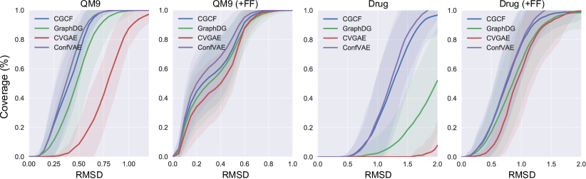
Figure 4: Curves of the Coverage score with different thresholds $\delta$ on GEOM-QM9 (left two) and GEOM-Drugs (right two) datasets. The first and third curves evaluates the generated conformations from different generative models, while the other two are further optimized with the empirical force field.

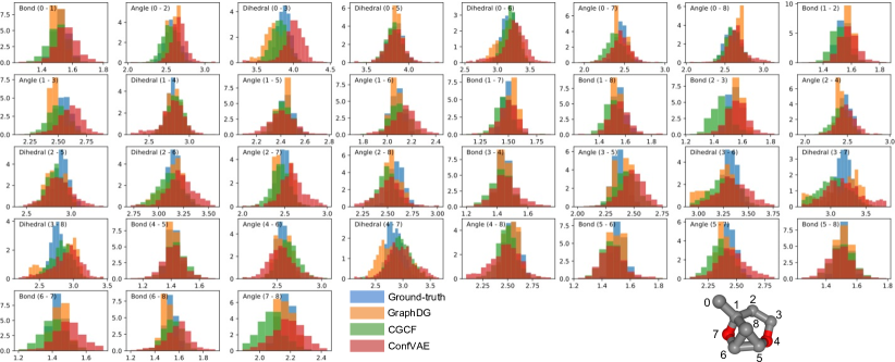
Figure 5: Marginal distributions $p(d_{uv}|{\mathcal{G}})$ of ground-truth and generated conformations from generative models. We study the edges between C and O atoms, and omit the H atoms for clarity. In each subplot, the annotation ($u-v$) denotes the corresponding atoms connected by the chemical bond $d_{uv}$.

In this section, we give more results about Coverage score with different thresholds $\delta$. The details about the COV score can be found in Sec. 4.2. Results are shown in Fig. 4. As shown in the figure, ConfVAE consistently achieves better performance than previous state-of-the-art models, which demonstrates our proposed method is capable to generate more realistic samples.

C.3 Visualization of Distributions

In Fig. 5, we investigate the accuracy of generated conformations by visualizing the marginal distributions $p(d_{uv}|{\mathcal{G}})$ for all pairwise distances between C and O atoms of a molecular graph in the ISO17 test set. As shown in the figure, though primarily designed for learning the 3D structures via an end-to-end framework, our method can still make a much better estimation of the distance distributions than the state-of-the-art model for molecular geometry modeling. As a representative element of the pairwise property between atoms, the inter-atomic distances demonstrate the capacity of our model to capture the inter-atomic interactions.

References

- Alipanahi et al. (2013) Alipanahi, B., Krislock, N., Ghodsi, A., Wolkowicz, H., Donaldson, L., and Li, M. Determining protein structures from noesy distance constraints by semidefinite programming. Journal of Computational Biology, 20(4):296–310, 2013.
- AlQuraishi (2019) AlQuraishi, M. End-to-end differentiable learning of protein structure. Cell systems, 8(4):292–301, 2019.
- Anand & Huang (2018) Anand, N. and Huang, P.-S. Generative modeling for protein structures. In Proceedings of the 32nd International Conference on Neural Information Processing Systems, pp. 7505–7516, 2018.
- Axelrod & Gomez-Bombarelli (2020) Axelrod, S. and Gomez-Bombarelli, R. Geom: Energy-annotated molecular conformations for property prediction and molecular generation. arXiv preprint arXiv:2006.05531, 2020.
- Ballard et al. (2015) Ballard, A. J., Martiniani, S., Stevenson, J. D., Somani, S., and Wales, D. J. Exploiting the potential energy landscape to sample free energy. Wiley Interdisciplinary Reviews: Computational Molecular Science, 5(3):273–289, 2015.
- Bengio (2000) Bengio, Y. Gradient-based optimization of hyperparameters. Neural computation, 12(8):1889–1900, 2000.
- Bennett et al. (2006) Bennett, K. P., Hu, J., Ji, X., Kunapuli, G., and Pang, J.-S. Model selection via bilevel optimization. In The 2006 IEEE International Joint Conference on Neural Network Proceedings, pp. 1922–1929. IEEE, 2006.
- Bottou (2010) Bottou, L. Large-scale machine learning with stochastic gradient descent. In Proceedings of COMPSTAT’2010, pp. 177–186. Springer, 2010.
- Bruna et al. (2013) Bruna, J., Zaremba, W., Szlam, A., and LeCun, Y. Spectral networks and locally connected networks on graphs. arXiv preprint arXiv:1312.6203, 2013.
- Chen et al. (2018) Chen, R. T., Rubanova, Y., Bettencourt, J., and Duvenaud, D. K. Neural ordinary differential equations. In Advances in neural information processing systems, pp. 6571–6583, 2018.
- Colson et al. (2007) Colson, B., Marcotte, P., and Savard, G. An overview of bilevel optimization. Annals of operations research, 153(1):235–256, 2007.
- Crippen et al. (1988) Crippen, G. M., Havel, T. F., et al. Distance geometry and molecular conformation, volume 74. Research Studies Press Taunton, 1988.
- De Vivo et al. (2016) De Vivo, M., Masetti, M., Bottegoni, G., and Cavalli, A. Role of molecular dynamics and related methods in drug discovery. Journal of medicinal chemistry, 59(9):4035–4061, 2016.
- Domke (2012) Domke, J. Generic methods for optimization-based modeling. In Artificial Intelligence and Statistics, pp. 318–326, 2012.
- Duvenaud et al. (2015) Duvenaud, D., Maclaurin, D., Aguilera-Iparraguirre, J., Gómez-Bombarelli, R., Hirzel, T., Aspuru-Guzik, A., and Adams, R. P. Convolutional networks on graphs for learning molecular fingerprints. arXiv preprint arXiv:1509.09292, 2015.
- Flamary et al. (2014) Flamary, R., Rakotomamonjy, A., and Gasso, G. Learning constrained task similarities in graphregularized multi-task learning. Regularization, Optimization, Kernels, and Support Vector Machines, pp. 103, 2014.
- Franceschi et al. (2017) Franceschi, L., Donini, M., Frasconi, P., and Pontil, M. Forward and reverse gradient-based hyperparameter optimization. arXiv preprint arXiv:1703.01785, 2017.
- Franceschi et al. (2018) Franceschi, L., Frasconi, P., Salzo, S., Grazzi, R., and Pontil, M. Bilevel programming for hyperparameter optimization and meta-learning. arXiv preprint arXiv:1806.04910, 2018.
- Gebauer et al. (2019) Gebauer, N., Gastegger, M., and Schütt, K. Symmetry-adapted generation of 3d point sets for the targeted discovery of molecules. In Advances in Neural Information Processing Systems, pp. 7566–7578, 2019.
- Gilmer et al. (2017) Gilmer, J., Schoenholz, S. S., Riley, P. F., Vinyals, O., and Dahl, G. E. Neural message passing for quantum chemistry. arXiv preprint arXiv:1704.01212, 2017.
- Gogineni et al. (2020) Gogineni, T., Xu, Z., Punzalan, E., Jiang, R., Kammeraad, J., Tewari, A., and Zimmerman, P. Torsionnet: A reinforcement learning approach to sequential conformer search. arXiv preprint arXiv:2006.07078, 2020.
- Gretton et al. (2012) Gretton, A., Borgwardt, K. M., Rasch, M. J., Schölkopf, B., and Smola, A. A kernel two-sample test. The Journal of Machine Learning Research, 13(1):723–773, 2012.
- Griewank & Walther (2008) Griewank, A. and Walther, A. Evaluating derivatives: principles and techniques of algorithmic differentiation. SIAM, 2008.
- Halgren (1996a) Halgren, T. A. Merck molecular force field. i. basis, form, scope, parameterization, and performance of mmff94. Journal of computational chemistry, 17(5-6):490–519, 1996a.
- Halgren (1996b) Halgren, T. A. Merck molecular force field. v. extension of mmff94 using experimental data, additional computational data, and empirical rules. Journal of Computational Chemistry, 17(5-6):616–641, 1996b.
- Hawkins (2017) Hawkins, P. C. Conformation generation: the state of the art. Journal of Chemical Information and Modeling, 57(8):1747–1756, 2017.
- Hoffmann & Noé (2019) Hoffmann, M. and Noé, F. Generating valid euclidean distance matrices. arXiv preprint arXiv:1910.03131, 2019.
- Hu et al. (2019) Hu, W., Liu, B., Gomes, J., Zitnik, M., Liang, P., Pande, V., and Leskovec, J. Strategies for pre-training graph neural networks. arXiv preprint arXiv:1905.12265, 2019.
- Ingraham et al. (2019) Ingraham, J., Riesselman, A. J., Sander, C., and Marks, D. S. Learning protein structure with a differentiable simulator. In International Conference on Learning Representations, 2019.
- Jumper et al. (2020) Jumper, J., Evans, R., Pritzel, A., Green, T., Figurnov, M., Tunyasuvunakool, K., Ronneberger, O., Bates, R., Zidek, A., Bridgland, A., et al. High accuracy protein structure prediction using deep learning. Fourteenth Critical Assessment of Techniques for Protein Structure Prediction (Abstract Book), 22:24, 2020.
- Kearnes et al. (2016) Kearnes, S., McCloskey, K., Berndl, M., Pande, V., and Riley, P. Molecular graph convolutions: moving beyond fingerprints. Journal of computer-aided molecular design, 30(8):595–608, 2016.
- Kingma & Welling (2013) Kingma, D. P. and Welling, M. Auto-encoding variational bayes. arXiv preprint arXiv:1312.6114, 2013.
- Kipf & Welling (2016) Kipf, T. N. and Welling, M. Semi-supervised classification with graph convolutional networks. arXiv preprint arXiv:1609.02907, 2016.
- Lemke & Peter (2019) Lemke, T. and Peter, C. Encodermap: Dimensionality reduction and generation of molecule conformations. Journal of chemical theory and computation, 15(2):1209–1215, 2019.
- Liberti et al. (2014) Liberti, L., Lavor, C., Maculan, N., and Mucherino, A. Euclidean distance geometry and applications. SIAM review, 56(1):3–69, 2014.
- Maclaurin et al. (2015) Maclaurin, D., Duvenaud, D., and Adams, R. Gradient-based hyperparameter optimization through reversible learning. In International Conference on Machine Learning, pp. 2113–2122, 2015.
- Mansimov et al. (2019) Mansimov, E., Mahmood, O., Kang, S., and Cho, K. Molecular geometry prediction using a deep generative graph neural network. arXiv preprint arXiv:1904.00314, 2019.
- Muñoz-González et al. (2017) Muñoz-González, L., Biggio, B., Demontis, A., Paudice, A., Wongrassamee, V., Lupu, E. C., and Roli, F. Towards poisoning of deep learning algorithms with back-gradient optimization. In Proceedings of the 10th ACM Workshop on Artificial Intelligence and Security, pp. 27–38, 2017.
- Noé et al. (2019) Noé, F., Olsson, S., Köhler, J., and Wu, H. Boltzmann generators: Sampling equilibrium states of many-body systems with deep learning. Science, 365(6457):eaaw1147, 2019.
- Paszke et al. (2019) Paszke, A., Gross, S., Massa, F., Lerer, A., Bradbury, J., Chanan, G., Killeen, T., Lin, Z., Gimelshein, N., Antiga, L., et al. Pytorch: An imperative style, high-performance deep learning library. arXiv preprint arXiv:1912.01703, 2019.
- Riniker & Landrum (2015) Riniker, S. and Landrum, G. A. Better informed distance geometry: using what we know to improve conformation generation. Journal of chemical information and modeling, 55(12):2562–2574, 2015.
- Scarselli et al. (2008) Scarselli, F., Gori, M., Tsoi, A. C., Hagenbuchner, M., and Monfardini, G. The graph neural network model. IEEE transactions on neural networks, 20(1):61–80, 2008.
- Schütt et al. (2017) Schütt, K., Kindermans, P.-J., Felix, H. E. S., Chmiela, S., Tkatchenko, A., and Müller, K.-R. Schnet: A continuous-filter convolutional neural network for modeling quantum interactions. In Advances in neural information processing systems, pp. 991–1001, 2017.
- Senior et al. (2020a) Senior, A. W., Evans, R., Jumper, J., Kirkpatrick, J., Sifre, L., Green, T., Qin, C., Žídek, A., Nelson, A. W., Bridgland, A., et al. Improved protein structure prediction using potentials from deep learning. Nature, 577(7792):706–710, 2020a.
- Senior et al. (2020b) Senior, A. W., Evans, R., Jumper, J., Kirkpatrick, J., Sifre, L., Green, T., Qin, C., Žídek, A., Nelson, A. W., Bridgland, A., et al. Improved protein structure prediction using potentials from deep learning. Nature, 577(7792):706–710, 2020b.
- Shi et al. (2020a) Shi, C., Xu, M., Guo, H., Zhang, M., and Tang, J. A graph to graphs framework for retrosynthesis prediction. In International Conference on Machine Learning, pp. 8818–8827. PMLR, 2020a.
- Shi et al. (2020b) Shi, C., Xu, M., Zhu, Z., Zhang, W., Zhang, M., and Tang, J. Graphaf: a flow-based autoregressive model for molecular graph generation. arXiv preprint arXiv:2001.09382, 2020b.
- Simm et al. (2020a) Simm, G., Pinsler, R., and Hernández-Lobato, J. M. Reinforcement learning for molecular design guided by quantum mechanics. In International Conference on Machine Learning, pp. 8959–8969. PMLR, 2020a.
- Simm & Hernández-Lobato (2020) Simm, G. N. and Hernández-Lobato, J. M. A generative model for molecular distance geometry. In International Conference on Machine Learning, 2020.
- Simm et al. (2020b) Simm, G. N., Pinsler, R., Csányi, G., and Hernández-Lobato, J. M. Symmetry-aware actor-critic for 3d molecular design. arXiv preprint arXiv:2011.12747, 2020b.
- Smith et al. (2020) Smith, D. G., Burns, L. A., Simmonett, A. C., Parrish, R. M., Schieber, M. C., Galvelis, R., Kraus, P., Kruse, H., Di Remigio, R., Alenaizan, A., et al. Psi4 1.4: Open-source software for high-throughput quantum chemistry. The Journal of chemical physics, 152(18):184108, 2020.
- Smith et al. (2017) Smith, J. S., Isayev, O., and Roitberg, A. E. Ani-1: an extensible neural network potential with dft accuracy at force field computational cost. Chemical science, 8(4):3192–3203, 2017.
- Wang et al. (2020) Wang, W., Yang, T., Harris, W. H., Gomez-Bombarelli, R., and Gómez-Bombarelli, R. Active learning and neural network potentials accelerate molecular screening of ether-based solvate ionic liquids. Chemical Communications, 56(63):8920, aug 2020. ISSN 1359-7345. URL https://pubs.rsc.org/en/content/articlehtml/2020/cc/d0cc03512bhttps://pubs.rsc.org/en/content/articlelanding/2020/cc/d0cc03512bhttp://pubs.rsc.org/en/Content/ArticleLanding/2020/CC/D0CC03512B.
- Xu et al. (2018) Xu, K., Hu, W., Leskovec, J., and Jegelka, S. How powerful are graph neural networks? arXiv preprint arXiv:1810.00826, 2018.
- Xu et al. (2021) Xu, M., Luo, S., Bengio, Y., Peng, J., and Tang, J. Learning neural generative dynamics for molecular conformation generation. In International Conference on Learning Representations, 2021. URL https://openreview.net/forum?id=pAbm1qfheGk.
- You et al. (2018) You, J., Liu, B., Ying, Z., Pande, V., and Leskovec, J. Graph convolutional policy network for goal-directed molecular graph generation. In Advances in neural information processing systems, pp. 6410–6421, 2018.