Composite Localization for Human Pose Estimation

Abstract

The existing human pose estimation methods are confronted with inaccurate long-distance regression or high computational cost due to the complex learning objectives. This work proposes a novel deep learning framework for human pose estimation called composite localization to divide the complex learning objective into two simpler ones: a sparse heatmap to find the keypoint’s approximate location and two short-distance offsetmaps to obtain its final precise coordinates. To realize the framework, we construct two types of composite localization networks: CLNet-ResNet and CLNet-Hourglass. We evaluate the networks on three benchmark datasets, including the Leeds Sports Pose dataset, the MPII Human Pose dataset, and the COCO keypoints detection dataset. The experimental results show that our CLNet-ResNet50 outperforms SimpleBaseline by 1.14% with about 1/2 GFLOPs. Our CLNet-Hourglass outperforms the original stacked-hourglass by 4.45% on COCO.

Index Terms—  Human pose estimation, Deep learning, Regression-based method, Heatmap-based method

1 Introduction

Human pose estimation, predicting a person’s body part or joint positions from an image or a video, is fundamental in computer vision with plenty of applications in human-computer interaction, action recognition, and other practical tasks. Recently, deep neural networks have surpassed the previous methods based on hand-crafted features by significantly improving the prediction accuracy in human pose estimation [1, 2, 3, 4].

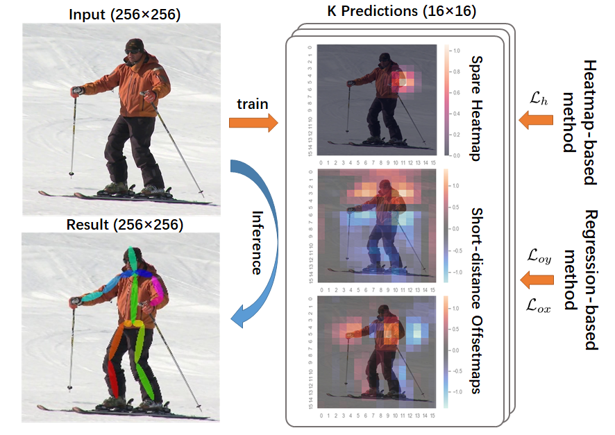
Fig. 1: Illustration of composite localization framework.

The human pose estimation based on deep learning can be divided into regression-based and heatmap-based methods. The regression-based method can predict the coordinates of keypoints in an end-to-end fashion but may sacrifice prediction accuracy due to the long-range information in the whole image [1, 5, 6]. The heatmap-based method predicts the probability of different keypoints on specific pixels and forms a heatmap to present the probabilities [7, 8, 9, 10, 11, 12], which usually produce higher prediction accuracy but require more computational resources for predicting the dense heatmap. Both types of methods have merits and limitations, such as inaccurate regression or high computational cost and complexity due to the complex learning objectives like long-distance regression or dense heatmap prediction. There are also a handful of studies that have attempted to combine the two types of methods, but they often fail to achieve satisfactory accuracy because they also ignore the complexity of learning objectives [13].

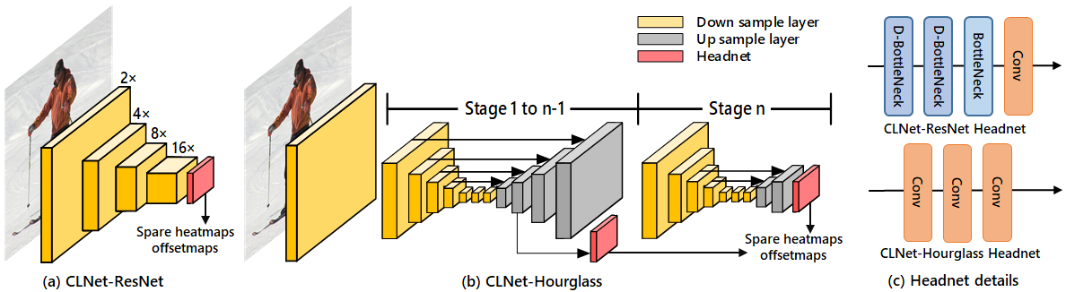
Fig. 2: Illustration of CLNet-ResNet and CLNet-Hourglass. ”D-BottleNeck” stands for the dilated bottleneck in  [14].

In this work, we find that the coordinates of keypoints can be divided into two simpler expressions: an approximate location and the corresponding short-distance regression. Accordingly, using a low-resolution heatmap (sparse heatmap) represents approximate locations to narrow the regression range. At the same time, regression-based method can be carried out short-distance regression from the approximate position. Such two simple objectives are suitable for neural networks to learn rather than a complex one [15]. Based on this, we propose a composite localization framework to predict sparse heatmaps and short-distance offsetmaps simultaneously. The main contributions can be summarized as follows: 1) We propose a composite localization framework (CL) for human pose estimation based on the two simple objectives and design the appropriate loss to improve performance. 2) We construct two types of composite localization networks, CLNet-ResNet and CLNet-Hourglass, based on our modified ResNet and Hourglass to show that our framework can be simply added to an existing model. 3) We evaluate CLNets on three benchmark datasets and show that CLNets achieve start-of-the-art performance and prove the rationality of framework design by sufficient ablation experiments.

2 Related Work

Early studies of human pose estimation have limited practical applications, primarily because they rely heavily on hand-crafted features [16]. Most recent work is based on deep learning and can be roughly divided into regression-based and heatmap-based methods. There are also some works trying to combine these two ideas for better performance.

Regression-based Method The first human pose estimation based on deep learning, DeepPose [1], proposes a cascaded deep neural network with extracting information evenly from the whole image to regress keypoints. Carreira et al. [5] use a self-correcting model to expand the expression ability of hierarchical feature extractors. Sun et al. [6] use bones to reparameterize the pose representation and joint connection structure to encode the long-range interactions in the specific posture. Although these methods improve the regression accuracy, they are still learning the complex goal of long-distance regression.

Heatmap-based Method Shortly after DeepPose was published, Tompson et al. [8] use heatmaps to represent the probabilities of keypoints in different locations. The stacked Hourglass architecture proposed by Newell et al. [9] uses repeated encode-decode structures with multiple supervision on intermediate heatmaps to improve the accuracy of the final prediction results. Many models [10, 17, 11, 12] continuously improve the performance of the classic stacked Hourglass network. Xiao et al. [3] propose simple but effective baseline methods, named SimpleBaseline. Chen et al. [18] use a two-stage strategy to further optimize the model for difficult samples. Sun et al. [4] maintain the high resolution of the model by training multi-resolution subnetworks. Although these models have good performance, learning complex dense heatmaps require complex network architecture and computational cost.

Composite Method A handful of works are also introduced to combine the regression-based and heatmap-based methods to overcome these methods’ shortcomings. Sun et al. [13] estimate the positions of keypoints as the integrals of all positions in the heatmaps to preserve the end-to-end differentiability. Papandreou et al. [2] solve a binary classification problem for each position, and all the positive locations need to predict offsets towards the keypoints.

3 Proposed Method

3.1 Composite Localization

As shown in Figure 1, the composite localization framework uses a sparse heatmap to find an approximate position and two corresponding offsetmaps to carry out short-distance regression.

Suppose the original image size is $W\times H$, the number of keypoints is $K$, and the sizes of sparse heatmaps and short-distance offsetmaps are $W^{\prime}\times H^{\prime}$. There are the following relationships: $W^{\prime}=\left\lfloor W/S\right\rfloor$ and $H^{\prime}=\left\lfloor H/S\right\rfloor$, where $S$ is the downsampling stride. Thus, each location in sparse heatmaps or short-distance offsetmaps corresponds to a patch of the original image with $S\times S$ size.

Sparse Heatmap For $K$ keypoints, there are $K$ sparse heatmaps, $\{\mathbf{H_{1}},\mathbf{H_{2}},...,\mathbf{H_{K}}\}$. Suppose the ground truth location of the $k$th keypoint in the original image is defined as $\mathbf{g}^{k}=(g_{x}^{k},g_{y}^{k}),g_{x}^{k}\in\{1...W\},g_{y}^{k}\in\{1...H\}$. The value at $\mathbf{p^{\prime}}=(p^{\prime}_{x},p^{\prime}_{y}),p^{\prime}_{x}\in\{1...W^{\prime}\},p^{\prime}_{y}\in\{1...H^{\prime}\}$ in $\mathbf{H_{k}}$ is defined as,

$$\mathbf{H_{k}}(\mathbf{p^{\prime}})=exp\begin{pmatrix}\frac{-\left\|t(\mathbf{p^{\prime}})-\mathbf{g}^{k}\right\|_{2}}{2\sigma^{2}}\end{pmatrix},$$ (1)

where $t(\mathbf{p^{\prime}})$ translates the location $\mathbf{p^{\prime}}=(p^{\prime}_{x},p^{\prime}_{y})$ in $\mathbf{H_{k}}$ to the center coordinates of the corresponding patch in the original image, which can be expressed as,

$$t(\mathbf{p^{\prime}})=\begin{pmatrix}(p^{\prime}_{x}-C)\times S,(p^{\prime}_{y}-C)\times S\end{pmatrix},$$ (2)

where $C$ is a deviation constant, equals to 0.5.

					val2017						test-dev2017
Method	Backbone	Pretrain	Input Size	GFLOPs	AP	$AP^{50}$	$AP^{75}$	$AP^{M}$	$AP^{L}$	AR	AP	$AP^{50}$	$AP^{75}$	$AP^{M}$	$AP^{L}$	AR
Hourglass  [9]	8 stacked hourglass	N	256$\times$192	14.3	71.9	91.0	80.0	69.3	77.1	77.5	-	-	-	-	-	-
CPN [18]	ResNet50	Y	256$\times$192	6.2	69.2	88.0	76.2	65.8	75.6	-	-	-	-	-	-	-
SimpleBaseline [3]	ResNet50	Y	256$\times$192	8.9	70.4	88.6	78.3	67.1	77.2	76.3	-	-	-	-	-	-
HRNet [4]	HRNet-W48	Y	256$\times$192	14.6	75.1	90.6	82.2	71.5	81.8	80.4	-	-	-	-	-	-
Integral Pose Regression [13]	ResNet101	Y	256$\times$256	11.0	-	-	-	-	-	-	67.8	88.2	74.8	63.9	74.0	-
Cai et al. [5]	ResNet50	N	256$\times$192	6.4	74.7	91.4	81.5	71.0	80.2	80.0	72.5	93.0	81.3	69.9	76.5	78.8
CLNet-ResNet	ResNet50	Y	256$\times$192	4.2	71.2	88.8	78.5	67.4	77.8	78.2	-	-	-	-	-	-
CLNet-Hourglass	8 stacked hourglass	N	256$\times$192	26.5	75.1	89.4	81.8	71.7	81.6	82.0	-	-	-	-	-	-
G-RMI [2]	ResNet101	Y	353$\times$257	57.0	-	-	-	-	-	-	64.9	85.5	71.3	62.3	70.0	69.7
CPN [18]	ResNet-Inception	Y	384$\times$288	-	72.2	89.2	78.6	68.1	79.3	-	72.1	91.4	80.0	68.7	77.2	78.5
SimpleBaseline [3]	ResNet152	Y	384$\times$288	35.6	74.3	89.6	81.1	70.5	81.6	79.7	73.7	91.9	82.8	71.3	80.0	79.0
HRNet [4]	HRNet-W32	Y	384$\times$288	16.0	75.8	90.6	82.5	72.0	82.7	80.9	74.9	92.5	82.8	71.3	80.9	80.1
HRNet [4]	HRNet-W48	Y	384$\times$288	32.9	76.3	90.8	82.9	72.3	83.4	81.2	75.5	92.5	83.3	71.9	81.5	80.5
CLNet-ResNet	ResNet50	Y	384$\times$288	9.5	73.4	89.1	79.9	69.4	80.0	79.7	-	-	-	-	-	-
CLNet-ResNet	ResNet101	Y	384$\times$288	17.7	74.2	89.3	80.5	70.2	81.0	80.5	-	-	-	-	-	-
CLNet-ResNet	ResNet152	Y	384$\times$288	25.9	74.9	89.7	81.4	70.9	81.9	81.1	74.1	91.5	81.5	70.4	80.1	80.3
CLNet-Hourglass	8 stacked hourglass	N	384$\times$256	52.9	76.5	89.8	82.8	72.9	82.9	82.6	75.8	91.7	83.2	72.4	81.4	82.0

Table 1: Comparisons of results on COCO val2017 and test-dev2017 set.

Short-distance Offsetmaps For $K$ keypoints, there are $2K$ offsetmaps, $\{\mathbf{O_{1}},\mathbf{O_{2}},...,\mathbf{O_{K}},\mathbf{O_{K+1}},...,\mathbf{O_{2K}}\}$, where the first $K$ and the last $K$ offsetmaps predict y-offsets and x-offsets, respectively. Similarly, for the ground truth location $\mathbf{g}^{k}$, the value at $\mathbf{p^{\prime}}=(p^{\prime}_{x},p^{\prime}_{y})$ in $\mathbf{O_{k}}$ and $\mathbf{O_{K+k}}$ can be defined as,

$$\left\{\begin{matrix}\mathbf{O_{k}}(\mathbf{p^{\prime}})&=\left(g_{y}^{k}-(p^{\prime}_{y}-C)\times S\right)/S,\\ \mathbf{O_{K+k}}(\mathbf{p^{\prime}})&=\left(g_{x}^{k}-(p^{\prime}_{x}-C)\times S\right)/S,\end{matrix}\right.$$ (3)

where $C$ and $S$ have the same meaning as above.

3.2 Network Design

We construct two networks to test the effectiveness and generalizability of our CL framework: CLNet-ResNet and CLNet-Hourglass.

CLNet-ResNet uses ResNet’s first four feature extraction stages [19] as its network backbone, as shown in Figure 2 (a). Inspired by Detnet [14], we sequentially add two dilated bottleneck layers, one bottleneck layer, and one convolutional layer to build the head subnetwork in CLNet-ResNet.

CLNet-Hourglass uses the classic stacked Hourglass [9] as its network backbone. As shown in Figure 2 (b), CLNet-Hourglass removes some up-sampling layers in the final stage and generates the predictions with appropriate resolution through the head subnetwork in each stage. The head subnetwork consists of three convolutional layers in series.

3.3 Loss Function Design

For sparse heatmap, let $\mathbf{H}_{k}$ and $\mathbf{\hat{H}}_{k}$ be the $k$th ground truth target and the $k$th keypoint prediction, respectively. The loss could be defined as,

$$\mathcal{L}_{h}=\frac{1}{K}\sum_{k=1}^{K}f(\mathbf{H}_{k},\hat{\mathbf{H}}_{k}),$$ (4)

where $f(\cdot)$ is the mean square error loss.

Offsetmaps only needs to learn about short-distance regression within a general region provided by sparse heatmaps, and its loss function can be expressed as follows,

$$\left\{\begin{matrix}\mathcal{L}_{oy}=\frac{1}{K}\sum_{k=1}^{K}\left(\frac{1}{N_{\mathbf{\Omega}}}\sum_{p^{\prime}\in\mathbf{\Omega}}g(\mathbf{O}_{k}(g^{\prime}),\hat{\mathbf{O}}_{k}(g^{\prime}))\right),\\ \mathcal{L}_{ox}=\frac{1}{K}\sum_{k=1}^{K}\left(\frac{1}{N_{\mathbf{\Omega}}}\sum_{p^{\prime}\in\mathbf{\Omega}}g(\mathbf{O}_{K+k}(g^{\prime}),\hat{\mathbf{O}}_{K+k}(g^{\prime}))\right),\end{matrix}\right.$$ (5)

where $\mathbf{\Omega}$ indicates $\hat{\mathbf{H}_{k}}(p^{\prime})\geq\tau$ with using threshold $\tau$ to control the range of regression. $g(\cdot)$ represents the smooth L1 loss. Note that the region may contain the approximate location of the keypoint and the location around it, which allows short-regression from adjacent approximate locations to improve the robustness of the model.

The overall loss function is,

$$\mathcal{L}=\omega_{h}\mathcal{L}_{h}+\mathcal{\omega}_{o}(\mathcal{L}_{oy}+\mathcal{L}_{ox}),$$ (6)

where $\omega_{h}$ and $\omega_{o}$ are the two parts’ weights..

3.4 Inference

There are three steps to parse sparse heatmaps and short-distance offsetmaps into 2d coordinates vector. For the $k$th keypoint, 1) the locations with high activation value ($\geq\tau$) in $\mathbf{H}_{k}$ were selected, and their center points were used as the initial locations of regression. 2) The values of $\mathbf{O}_{k}$ and $\mathbf{O}_{K+k}$ in the corresponding locations are used as y-offset and x-offset to obtain the $k$th keypoint’s coordinates. 3) The predicted coordinates are weighted average according to their activation values on $\mathbf{H}_{k}$ to obtain a final predicted coordinate about the $k$th keypoint.

4 Experiments

	Head	Sho.	Elb.	Wri.	Hip	Knee	Ank.	PCKh@0.5
Tompson et al. [7]	95.8	90.3	80.5	74.3	77.6	69.7	62.8	79.6
Carreira et al. [5]	95.7	91.7	81.7	72.4	82.8	73.2	66.4	81.3
Newell et al. [9]	98.2	96.3	91.2	87.1	90.1	87.4	83.6	90.9
Yang et al.∗ [10]	98.5	96.7	92.5	88.7	91.1	88.6	86.0	92.0
Ke et al.∗ [17]	98.5	96.8	92.7	88.4	90.6	89.4	86.3	92.1
Tang et al.∗ [11]	98.4	96.9	92.6	88.7	91.8	89.4	86.2	92.3
Xiao et al. [3]	98.5	96.6	91.9	87.6	91.1	88.1	84.1	91.5
Sekii [20]	97.9	95.3	89.1	83.5	87.9	82.7	76.2	88.1
Zhang et al. [21]	98.3	96.4	91.5	87.4	90.9	87.1	83.7	91.1
Sun et al. [4]	98.6	96.9	92.8	89.0	91.5	89.0	85.7	92.3
Tang et al.∗ [12]	98.7	97.1	93.1	89.4	91.9	90.1	86.7	92.7
Artacho et al. [22]	-	-	-	-	-	-	-	92.7
CLNet-ResNet50	98.2	95.9	90.5	85.9	90.4	86.6	82.0	90.4
CLNet-Hourglass	98.4	96.6	92.4	88.4	90.9	89.4	84.8	91.9

Table 2: Comparisons of results on the MPII test set. ”*” means using multi-scale image pyramids as input.

	# Param	FLOPs	FPS	FPS’	PCKh@0.5
8-stacked Hourglass, ECCV’16 [9]	26M	55G	20	70	90.9
PyraNet, ICCV’17∗ [10]	28M	46G	6	40	92.0
SimpleBaseline, ECCV’18 [3]	69M	23G	60	202	91.5
PPN, ECCV’18 [20]	16M	6G	388	728	88.1
HRNet, CVPR’19 [4]	64M	21G	29	283	92.3
FPD, CVPR’19 [21]	3M	9G	40	250	91.1
UniPose, CVPR’20 [22]	47M	15G	41	210	92.7
CLNet-ResNet50	13.5M	5.6G	136	571	90.4

Table 3: Comparisons of complexity. FPS are calculated with batch size one, while FPS’ are calculated using full GPU memory. ”*” means using multi-scale image pyramids.

4.1 Experiment Setup

Datasets LSP and its extended training set provide 11k training images and 1k testing images [23], and MPII [24] provides around 25k images with 40K person instances for single-person. MS COCO dataset [25] requires localization of multi-person keypoints in the wild. COCO train2017 set includes 120K images and 150K person instances, while val2017 set and test-dev2017 set include 5K images with 6K person instances and 20K images, respectively.

Evaluation Protocol We use the Percentage of Correct Keypoints (PCK) [24] as the evaluation metric for single-person human pose estimation. The normalized distance is torso size for LSP while a fraction of the head size (referred to as PCKh) for MPII. For the MS COCO dataset, object keypoint similarity (OKS) based mAP is used as an evaluation metric.

Implementation Details The size of the input image is 256 $\times$ 256 for LSP and MPII by convention. The input size for COCO varies among experiments. The standard deviation $\sigma$ in sparse heatmaps is 16, and the threshold $\tau$ is 0.6. The loss weight of $\omega_{h}$ and $\omega_{o}$ is 0.5 and 2, respectively. Training data are augmented by shearing, scaling, rotation, flipping as reported in [9, 11, 3]. The networks are trained using PyTorch [26]. We optimize the models via Adam [27] with a batch size of 128 for 140 epochs. The learning rate is initialized as $1\times 10^{-3}$ and then dropped by a factor of 10 at the 90th and 120th epochs for CLNet-ResNet. For CLNet-Hourglass, we follow the same hyper-parameters and settings in [9]. For top-down multi-person human pose estimation in COCO, we use the same detector as SimpleBaseline [3] and HRNet [4].

	Head	Sho.	Elb.	Wri.	Hip	Knee	Ank.	PCK@0.2
Tompson et al. [7]	90.6	79.2	67.9	63.4	69.5	71.0	64.2	72.3
Yang et al.∗ [10]	98.3	94.5	92.2	88.9	94.4	95.0	93.7	93.9
Tang et al.∗ [11]	97.5	95.0	92.5	90.1	93.7	95.2	94.2	94.0
Tang et al.∗ [12]	98.6	95.4	93.3	89.8	94.3	95.7	94.4	94.5
Artacho et al. [22]	-	-	-	-	-	-	-	94.5
CLNet-ResNet50	98.6	95.2	94.1	92.5	95.5	95.2	93.1	94.9
CLNet-Hourglass	98.5	96.3	95.4	94.6	96.7	96.0	94.3	96.0

Table 4: Comparisons of results on the LSP test set. ”*” means using multi-scale image pyramids as input.

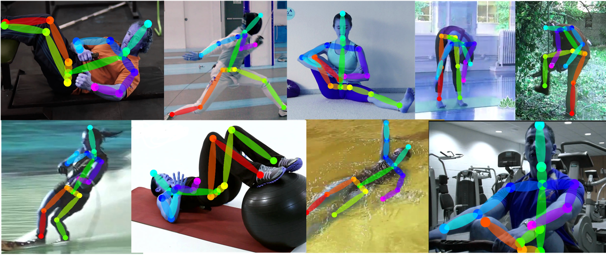
Fig. 3: The random qualitative results on MPII test set.

4.2 Comparison with State-of-the-art Methods

Results on COCO As shown in Table 1, on the COCO val2017 set, CLNet-ResNet50 achieves a 71.2 AP score with the input size 256$\times$192, and outperforms SimpleBaseline-ResNet50 by 1.14% with near 1/2 FLOPs. CLNet-Hourglass, trained from scratch, achieves a 75.1 AP score and obtains 3.2 points improvement compared with the original Hourglass. As for the input size 384 $\times$ 288, CLNet-ResNet outperforms SimpleBaseline and CL-Hourglass outperforms the HRNet while original Hourglass is not as good as other methods. On test-dev 2017 set, CLNet-ResNet152 outperforms SimpleBaseline-ResNet152 0.4 points. CLNet-Hourglass outperforms all others with a 75.8 AP score.

Results on MPII Table 2 shows our results on the MPII test. Furthermore, we compare the complexity of CLNet-ResNet50 and the most popular methods on the MPII test set in Table 3. We measure the speed and latency by float-point operations (FLOPs) and frames-per-second (FPS). As shown in Table 3, FPD [21] has much fewer FLOPs than SimpleBaseline [3] but is slower, and has comparable FLOPs with PPN [20] but is much slower. Our method achieves an excellent trade-off between efficiency and effectiveness. Our CLNet-ResNet50 is approximately two times slower than PPN but has higher accuracy, while it has comparable accuracy but surpasses the others in terms of FPS by a large margin. Figure 3 shows the visualization of CLnet-Resnet50 on the MPII test set.

Results on LSP Table 4 shows the results of CLNets and the most popular methods on the LSP test set. Our results are the new state-of-the-art.

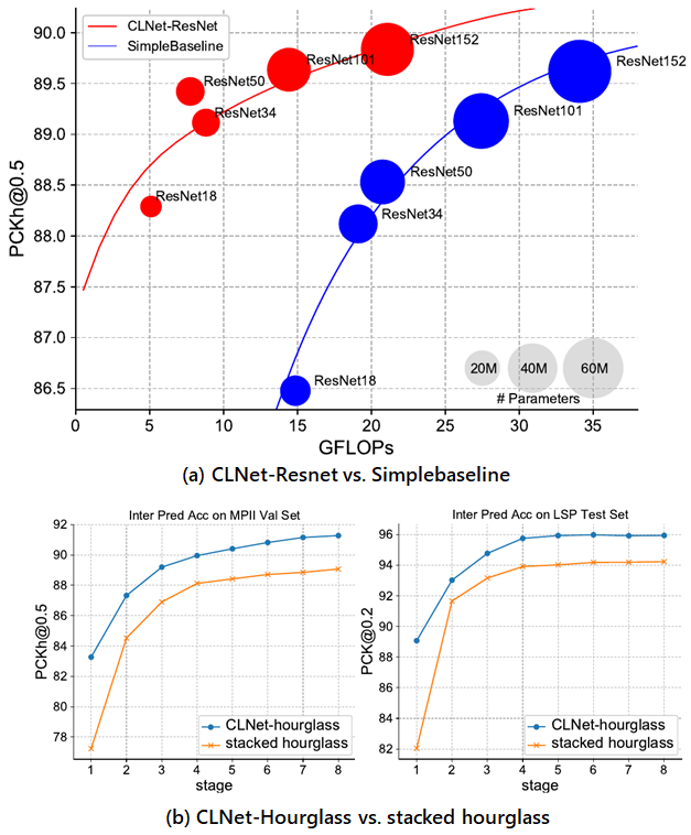
Fig. 4: Comparisons of accuracy at different stages of the network on our CLNet-hourglass and stacked hourglass network on MPII validation set (left) and LSP test set (right).

4.3 Ablation Study

Influence of the downsampling stride Different downsampling stride $S$ will make the range of short-distance regression different and the model’s complexity different, which may significantly influence the result. We do experiments with different values of $S$. As Table 5 showed, the 8 $\times$8 heatmap has the most parameters because of the vast channel numbers in the last stage, while 16$\times$16 heatmap achieves the best results with the fewest parameters.

stride $S$	Heatmap Size	Params	PCK@0.2
4	64x64	16.8M	92.2
8	32x32	15.7M	93.9
16	16x16	13.4M	94.9
32	8x8	28.9M	93.4

Table 5: Comparisons of results on the LSP test set with different downsampling stride $S$.

Influence of Loss Function We consider the effect of two other loss functions. The first calculates the MSE loss on offsetmaps where the corresponding position in the heatmap is the peak and keeps the heatmap loss the same as traditional Gaussian heatmap loss with a 93.2 score. The second is the loss function used in G-RMI [2], which solves a binary classification problem for heatmap and calculates each positive location has offset the loss with a 93.7 score. Our loss function helps the models achieve the best score of 94.9.

Cost-effectiveness Analysis As shown in Figure4 (a), we test different backbone networks in design. The performance continued to improve as the network deepens. SimpleBaseline is a baseline for effectiveness and efficiency verification of CLNet-ResNet due to the most similar architecture. CLNet-ResNet outperforms the SimpleBaseline in all backbones. Using the same backbone, CLNet-ResNet has fewer GFLOPs and parameters than SimpleBaselines because our networks do not have any up-sampling layer and the last stage with vast channels in ResNet. The gap goes from 0.2% to 1.8% when the backbone changes from ResNet152 to ResNet18. It demonstrates that our method can use the features more efficiently.

Generalization Our method can also be used in other popular models. We do our generalization experiments on the stacked hourglass network, named CLNet-hourglass. Although it is not very elegant compared with CLNet-ResNet, it dramatically improves performance (about 2%) on two commonly used single-person pose estimation benchmarks, as shown in Figure 4 (b). Especially, CLNet-hourglass surpasses the original stacked hourglass network on the first stage by a large margin (relative 8.5% on MPII validation set and 8.0% on LSP test set), indicating our method can using features more effectively again.

5 Conclusion

In this paper, we has proposed the composite localization for human pose estimation, dividing the complex learning objective into two simpler ones and a combined heatmap-based and regression-based method to solve them. Besides, we have constructed two types of CLNets with different backbones and design appropriate loss functions. With fewer parameters than their plain counterparts, CLNets have achieved better average precision on three standard benchmark datasets, proving our framework’s effectiveness and generalizability. We expect to optimize the CL framework and design a more elegant and powerful network in future work.

References

- [1] Alexander Toshev and Christian Szegedy, “Deeppose: Human pose estimation via deep neural networks,” in Proceedings of the IEEE conference on computer vision and pattern recognition, 2014, pp. 1653–1660.
- [2] George Papandreou, Tyler Zhu, Nori Kanazawa, Alexander Toshev, Jonathan Tompson, Chris Bregler, and Kevin Murphy, “Towards accurate multi-person pose estimation in the wild,” in The IEEE Conference on Computer Vision and Pattern Recognition (CVPR), July 2017.
- [3] Bin Xiao, Haiping Wu, and Yichen Wei, “Simple baselines for human pose estimation and tracking,” in Proceedings of the European Conference on Computer Vision (ECCV), 2018, pp. 466–481.
- [4] Ke Sun, Bin Xiao, Dong Liu, and Jingdong Wang, “Deep high-resolution representation learning for human pose estimation,” in The IEEE Conference on Computer Vision and Pattern Recognition (CVPR), June 2019.
- [5] Joao Carreira, Pulkit Agrawal, Katerina Fragkiadaki, and Jitendra Malik, “Human pose estimation with iterative error feedback,” in Proceedings of the IEEE conference on computer vision and pattern recognition, 2016, pp. 4733–4742.
- [6] Xiao Sun, Jiaxiang Shang, Shuang Liang, and Yichen Wei, “Compositional human pose regression,” in Proceedings of the IEEE International Conference on Computer Vision, 2017, pp. 2602–2611.
- [7] Jonathan J Tompson, Arjun Jain, Yann LeCun, and Christoph Bregler, “Joint training of a convolutional network and a graphical model for human pose estimation,” in Advances in neural information processing systems, 2014, pp. 1799–1807.
- [8] Jonathan Tompson, Ross Goroshin, Arjun Jain, Yann LeCun, and Christoph Bregler, “Efficient object localization using convolutional networks,” in The IEEE Conference on Computer Vision and Pattern Recognition (CVPR), June 2015.
- [9] Alejandro Newell, Kaiyu Yang, and Jia Deng, “Stacked hourglass networks for human pose estimation,” in European conference on computer vision. Springer, 2016, pp. 483–499.
- [10] Wei Yang, Shuang Li, Wanli Ouyang, Hongsheng Li, and Xiaogang Wang, “Learning feature pyramids for human pose estimation,” in The IEEE International Conference on Computer Vision (ICCV), Oct 2017.
- [11] Wei Tang, Pei Yu, and Ying Wu, “Deeply learned compositional models for human pose estimation,” in The European Conference on Computer Vision (ECCV), September 2018.
- [12] Jingwei Tang, Yagiz Aksoy, Cengiz Oztireli, Markus Gross, and Tunc Ozan Aydin, “Learning-based sampling for natural image matting,” in The IEEE Conference on Computer Vision and Pattern Recognition (CVPR), June 2019.
- [13] Xiao Sun, Bin Xiao, Fangyin Wei, Shuang Liang, and Yichen Wei, “Integral human pose regression,” in The European Conference on Computer Vision (ECCV), September 2018.
- [14] Zeming Li, Chao Peng, Gang Yu, Xiangyu Zhang, Yangdong Deng, and Jian Sun, “Detnet: Design backbone for object detection,” in The European Conference on Computer Vision (ECCV), September 2018.
- [15] Zhanghan Ke, Kaican Li, Yurou Zhou, Qiuhua Wu, Xiangyu Mao, Qiong Yan, and Rynson WH Lau, “Is a green screen really necessary for real-time human matting?,” arXiv preprint arXiv:2011.11961, 2020.
- [16] Yi Yang and Deva Ramanan, “Articulated human detection with flexible mixtures of parts,” IEEE transactions on pattern analysis and machine intelligence, vol. 35, no. 12, pp. 2878–2890, 2012.
- [17] Lipeng Ke, Ming-Ching Chang, Honggang Qi, and Siwei Lyu, “Multi-scale structure-aware network for human pose estimation,” in The European Conference on Computer Vision (ECCV), September 2018.
- [18] Yilun Chen, Zhicheng Wang, Yuxiang Peng, Zhiqiang Zhang, Gang Yu, and Jian Sun, “Cascaded pyramid network for multi-person pose estimation,” in Proceedings of the IEEE Conference on Computer Vision and Pattern Recognition, 2018, pp. 7103–7112.
- [19] Kaiming He, Xiangyu Zhang, Shaoqing Ren, and Jian Sun, “Deep residual learning for image recognition,” in Proceedings of the IEEE conference on computer vision and pattern recognition, 2016, pp. 770–778.
- [20] Taiki Sekii, “Pose proposal networks,” in Proceedings of the European Conference on Computer Vision (ECCV), 2018, pp. 342–357.
- [21] Feng Zhang, Xiatian Zhu, and Mao Ye, “Fast human pose estimation,” in The IEEE Conference on Computer Vision and Pattern Recognition (CVPR), June 2019.
- [22] Bruno Artacho and Andreas Savakis, “Unipose: Unified human pose estimation in single images and videos,” in Proceedings of the IEEE/CVF Conference on Computer Vision and Pattern Recognition, 2020, pp. 7035–7044.
- [23] Sam Johnson and Mark Everingham, “Clustered pose and nonlinear appearance models for human pose estimation,” in Proceedings of the British Machine Vision Conference, 2010, doi:10.5244/C.24.12.
- [24] Mykhaylo Andriluka, Leonid Pishchulin, Peter Gehler, and Bernt Schiele, “2d human pose estimation: New benchmark and state of the art analysis,” in The IEEE Conference on Computer Vision and Pattern Recognition (CVPR), June 2014.
- [25] Tsung-Yi Lin, Michael Maire, Serge Belongie, James Hays, Pietro Perona, Deva Ramanan, Piotr Dollár, and C Lawrence Zitnick, “Microsoft coco: Common objects in context,” in European conference on computer vision. Springer, 2014, pp. 740–755.
- [26] Benoit Steiner, Zachary DeVito, Soumith Chintala, Sam Gross, Adam Paszke, Francisco Massa, Adam Lerer, Gregory Chanan, Zeming Lin, Edward Yang, Alban Desmaison, Alykhan Tejani, Andreas Kopf, James Bradbury, Luca Antiga, Martin Raison, Natalia Gimelshein, Sasank Chilamkurthy, Trevor Killeen, Lu Fang, and Junjie Bai, “Pytorch: An imperative style, high-performance deep learning library,” in Advances in Neural Information Processing Systems 32, 2019.
- [27] Diederik P. Kingma and Jimmy Ba, “Adam: A method for stochastic optimization,” 2015.