Causal effect on a target population: a sensitivity analysis to handle missing covariates

Abstract

Randomized Controlled Trials (RCTs) are often considered the gold standard for estimating causal effect, but they may lack external validity when the population eligible to the RCT is substantially different from the target population. Having at hand a sample of the target population of interest allows us to generalize the causal effect. Identifying the treatment effect in the target population requires covariates to capture all treatment effect modifiers that are shifted between the two sets. Standard estimators then use either weighting (IPSW), outcome modeling (G-formula), or combine the two in doubly robust approaches (AIPSW). However such covariates are often not available in both sets. In this paper, after proving $L^{1}$-consistency of these three estimators, we compute the expected bias induced by a missing covariate, assuming a Gaussian distribution, a continuous outcome, and a semi-parametric model. Under this setting, we perform a sensitivity analysis for each missing covariate pattern and compute the sign of the expected bias. We also show that there is no gain in linearly imputing a partially-unobserved covariate. Finally we study the substitution of a missing covariate by a proxy. We illustrate all these results on simulations, as well as semi-synthetic benchmarks using data from the Tennessee Student/Teacher Achievement Ratio (STAR), and a real-world example from critical care medicine.
Keywords: Average treatment effect (ATE); distributional shift; external validity; generalizability; transportability.

This article has been accepted for publication in Journal of Causal Inference.
Updated version is available on degruyter website.

1 Introduction

Context

Randomized Controlled Trials (RCTs) are often considered the gold standard for estimating causal effects (Imbens and Rubin, 2015). Yet, they may lack external validity, when the population eligible to the RCT is substantially different from the target population of the intervention policy (Rothwell, 2005). Indeed, if there are treatment effect modifiers with a different distribution in the target population than that in the trial, some form of adjustment of the causal effects measured on the RCT is necessary to estimate the causal effect in the target population. Using covariates present in both RCT and an observational sample of the target population, this target population average treatment effect (ATE) can be identified and estimated with a variety of methods (Imbens et al., 2005; Cole and Stuart, 2010; Stuart et al., 2011; Pearl and Bareinboim, 2011; Bareinboim and Pearl, 2013; Tipton, 2013; Bareinboim et al., 2014; Pearl and Bareinboim, 2014; Kern et al., 2016; Bareinboim and Pearl, 2016; Buchanan et al., 2018; Stuart et al., 2018; Dong et al., 2020), reviewed in (Colnet et al., 2020) and (Degtiar and Rose, 2021).

In this context, two main approaches exist to estimate the target population ATE from a RCT. The Inverse Probability of Sampling Weighting (IPSW) reweights the RCT sample so that it resembles the target population with respect to the necessary covariates for generalization, while the G-formula models the outcome, using the RCT sample, with and without treatment conditionally on the same covariates, and then marginalizes the model to the target population of interest. These two methods can be combined in a doubly-robust approach –Augmented Inverse Probability of Sampling Weighting (AIPSW)– which enjoys better statistical properties. These methods rely on covariates to capture the heterogeneity of the treatment and the population distributional shift. But the datasets describing the RCT and the target population are seldom acquired as part of a homogeneous effort and as a result they come with different covariates (Pearl and Bareinboim, 2011; Susukida et al., 2016; Lesko et al., 2016; Stuart and Rhodes, 2017; Egami and Hartman, 2021; Li et al., 2021). Restricting the analysis to the covariates in common raises the risk of omitting an important one leading to identifiability issues. Controlling biases due to unobserved covariates is of crucial importance for causal inference, where it is known as sensitivity analysis (Cornfield et al., 1959; Imbens, 2003; Rosenbaum, 2005).

Prior work

The problem of missing covariates is central in causal inference as, in an observational study, one can never prove that there is no hidden confounding. In that setting, sensitivity analysis strives to assess how far confounding would affect the conclusion of a study (for example, would the ATE be of a different sign with such a hidden confounder). Such approaches date back to a study on the effect of smoking on lung cancer (Cornfield et al., 1959), and have been further developed for both parametric (Imbens, 2003; Rosenbaum, 2005; Dorie et al., 2016; Ichino et al., 2008; Cinelli and Hazlett, 2020) and semi-parametric situations (Franks et al., 2019; Veitch and Zaveri, 2020). Typically, the analysis translates expert judgment into mathematical expression of how much the confounding affects treatment assignment and the outcome, and finally how much the estimated treatment effect is biased. In practice the expert must usually provide sensitivity parameters that reflect plausible properties of the missing confounder. Classic sensitivity analysis, dedicated to ATE estimation from observational data, use as sensitivity parameters the impact of the missing covariate on treatment assignment probability along with the strength on the outcome of the missing confounder. However, given that these quantities are hardly directly transposable when it comes to generalization, these approaches cannot be directly applied to estimate the population treatment effect. These parameters have to be respectively replaced by the covariate shift and the strength of a treatment effect modifier. Existing sensitivity analysis methods for generalization usually consider a completely unobserved covariate. (Andrews and Oster, 2019) rely on a logistic model for sampling probability and a linear generative model of the outcome. (Dahabreh et al., 2019) propose a sensitivity analysis assuming a model on the identification bias of the conditional average treatment effect. Very recent works propose two other approaches: (i) (Nie et al., 2021) rely on the IPSW estimator and bound the error on the the density ratio and then derive the bias on the ATE following the spirit of (Rosenbaum, 2005); (ii) (Huang et al., 2021) present a method with very few assumptions on the data generative process leading to three sensitivity parameters, including the variance of the treatment effect. As the analysis starts from two data sets, the missing covariate can also be partially observed in one of the two data set, which opens the door to new dedicated methods, in addition to sensitivity methods for totally-missing covariates. Following this observation, (Nguyen et al., 2017, 2018) handle the case where a covariate is present in the RCT but not in the observational data set, and establish a sensitivity analysis under the hypothesis of a linear generative model for the outcome. When the missing covariate is partially observed, practitioners sometimes impute missing values based on other observed covariates, though this approach is poorly documented. For example, (Lesko et al., 2016) impute a partially-observed covariate in a clinical study using a range of plausible distributions. Imputation has also been used in the context of individual participant data in meta-analysis (Resche-Rigon et al., 2013; Jolani et al., 2015).

Contributions

In this work we investigate the problem of a missing covariate that affects the identifiability of the target population average treatment effect (ATE), a common situation when combining different data sources. This work comes after the identifiability assessment, that is we consider that the necessary set of covariates to generalize is known, but a necessary covariate is totally or partially missing. Section 2 recalls the context along with the generic notations and assumptions used when coming to generalization. In Section 3, we quantify the bias due to unobserved covariates under the assumption of a semi-parametric generative process, considering a linear conditional average treatment effect (CATE), and under a transportability assumption of links between covariates in both populations. This bias is not estimator-specific and remains valid for the IPSW, G-formula, and AIPSW estimators. We also prove that a linear imputation of a partially missing covariate can not replace a sensitivity analysis. As mentioned in the introduction, and unlike classic sensitivity analysis, several missing data patterns can be observed: either totally missing or missing in one of the two sets. Therefore Section 3 provides sensitivity analysis frameworks for all the possible missing data patterns, including the case of a proxy variable that would replace the missing one. These results can be useful for users as they may be tempted to consider the intersection of common covariates between the RCT and the observational data. We detail how the different patterns involve either one or two sensitivity parameters. To give users an interpretable analysis, and due to the specificity of the sensitivity parameters at hands, we propose an adaptation of sensitivity maps (Imbens, 2003) that are commonly used to communicate sensitivity analysis results. Section 4 presents an extensive synthetic simulation analysis that illustrates theoretical results along with a semi-synthetic data simulation using the Tennessee Student/Teacher Achievement Ratio (STAR) experiment evaluating the effect of class size on children performance in elementary schools (Krueger, 1999). Finally, Section 5 provides a real-world analysis to assess the effect of acid tranexomic on the Disability Rating Score (DRS) for trauma patients when a covariate is totally missing.

2 Problem setting: generalizing a causal effect

This section recalls the complete case context and identification assumptions. Any reader familiar with the notations and willing to jump to the sensitivity analysis can directly go to Section 3.

2.1 Notations

Notations are grounded on the potential outcome framework (Imbens and Rubin, 2015). We model each observation in the RCT or observational population as described by a random tuple $(X_{i},Y_{i}(0),Y_{i}(1),A_{i},S_{i})$ for $i\in\{1,\ldots,n\}$ drawn from a distribution $\left(X,Y(0),Y(1),A,S\right)\in\mathbb{R}^{p}\times\mathbb{R}^{2}\times\{0,1\}^{2}$, such that the observations are iid. For each observation, $X_{i}$ is a $p$-dimensional vector of covariates, $A_{i}$ denotes the binary treatment assignment (with $A_{i}=1$ if treated and $A_{i}=0$ otherwise), $Y_{i}(a)$ is the continuous outcome had the subject been given treatment $a$ (for $a\in\{0,1\}$), and $S_{i}$ is a binary indicator for RCT eligibility (i.e., meet the RCT inclusion and exclusion criteria) and willingness to participate if being invited to the trial ($S_{i}=1$ if eligible and $S_{i}=0$ if not). Assuming consistency of potential outcomes, and no interference between treated and non-treated subject (SUTVA assumption), we denote by $Y_{i}=A_{i}Y_{i}(1)+(1-A_{i})Y_{i}(0)$ the observed outcome under treatment assignment $A_{i}$.

Assuming the potential outcomes are integrable, we define the conditional average treatment effect (CATE):

$$\forall x\in\mathcal{X}\,,\quad\tau(x)=\mathbb{E}\left[Y(1)-Y(0)\mid X=x\right]\,,$$

and the population average treatment effect (ATE):

$$\tau=\mathbb{E}\left[Y(1)-Y(0)\right]=\mathbb{E}\left[\tau(X)\right]\,.$$

Unless explicitly stated, all expectations are taken with respect to all variables involved in the expression. We model the patients belonging to an RCT sample of size $n$ and in an observational data sample of size $m$ by $n+m$ independent random tuples: $\{X_{i},Y_{i}(0),Y_{i}(1),A_{i},S_{i}\}_{i=1}^{n+m},$ where the RCT samples $i=1,\ldots,n$ are identically distributed according to $\mathcal{P}(X,Y(0),Y(1),A,S\mid S=1)$, and the observational data samples $i=n+1,\ldots,n+m$ are identically distributed according to $\mathcal{P}(X,Y(0),Y(1),A,S)$. We also denote $\mathcal{R}=\{1,\ldots,n\}$ the index set of units observed in the RCT study, and $\mathcal{O}=\{n+1,\ldots,n+m\}$ the index set of units observed in the observational study.
For each RCT sample $i\in\mathcal{R}$, we observe $(X_{i},A_{i},Y_{i},S_{i}=1)$, while for observational data $i\in\mathcal{O}$, we consider the setting where we only observe the covariates $X_{i}$, which is a common case in practice. A typical data set is presented on Table 1.

Because the RCT sample and observational data do not follow the same covariate distribution, the ATE $\tau$ is different from the RCT’s (or sample) average treatment effect $\tau_{1}$ which can be expressed as:

$$\tau\neq\tau_{1},\quad\text{where}\;\tau_{1}:=\mathbb{E}[Y(1)-Y(0)\mid S=1]\,.$$

This difference is the core of the lack of external validity introduced in the beginning of the work, but formalized with a mathematical expression. Throughout the paper, we denote $\mu_{a}(x):=\mathbb{E}\left[Y(a)\mid X=x\right]$ the conditional mean outcome under treatment $a\in\{0,1\}$ (also called responses surfaces). and $e_{1}(x):=\mathbb{P}(A=1\mid X=x,S=1)$ the propensity score in the RCT population. This function is imposed by the trial characteristics and is usually a constant denoted by $e_{1}$ (other cases include stratified RCT trials).

For notational clarity, estimators are indexed by the number of observations used for their computation. For instance, response surfaces can be estimated using controls and treated individuals in the RCT to obtain respectively $\hat{\mu}_{0,n}$ and $\hat{\mu}_{1,n}$. Similarly, we denote by $\hat{\tau}_{n}$ an estimator of $\tau$ depending only on the RCT samples (for example the difference-in-means estimator), and by $\hat{\tau}_{n,m}$ an estimator computed using both datasets.

2.2 Identifiability (or causal) assumptions

The consistency of treatment assignment assumption ($Y=AY(1)+(1-A)Y(0)$) has already been introduced in Section 2. To ensure the internal validity of the RCT, we need to assume randomization of treatment assignment and positivity of trial treatment assignment.

Assumption 1 (Treatment randomization within the RCT).

$\forall a\in\{0,1\},\,Y(a)\mathchoice{\mathrel{\hbox to0.0pt{$\displaystyle\perp$\hss}\mkern 2.0mu{\displaystyle\perp}}}{\mathrel{\hbox to0.0pt{$\textstyle\perp$\hss}\mkern 2.0mu{\textstyle\perp}}}{\mathrel{\hbox to0.0pt{$\scriptstyle\perp$\hss}\mkern 2.0mu{\scriptstyle\perp}}}{\mathrel{\hbox to0.0pt{$\scriptscriptstyle\perp$\hss}\mkern 2.0mu{\scriptscriptstyle\perp}}}A\mid S=1,X$.

In some cases, the trial is said to be completely randomized, that is $\forall a\in\{0,1\},\,Y(a)\mathchoice{\mathrel{\hbox to0.0pt{$\displaystyle\perp$\hss}\mkern 2.0mu{\displaystyle\perp}}}{\mathrel{\hbox to0.0pt{$\textstyle\perp$\hss}\mkern 2.0mu{\textstyle\perp}}}{\mathrel{\hbox to0.0pt{$\scriptstyle\perp$\hss}\mkern 2.0mu{\scriptstyle\perp}}}{\mathrel{\hbox to0.0pt{$\scriptscriptstyle\perp$\hss}\mkern 2.0mu{\scriptscriptstyle\perp}}}A\mid S=1$, thus removing any potential stratification of the treatment assignment.

Assumption 2 (Positivity of trial treatment assignment).

$\exists\eta_{1}>0,\forall x\in\mathcal{X},\eta_{1}\leq e_{1}(x)\leq 1-\eta_{1}$

Under these two assumptions, along with the SUTVA assumption (see, e.g., Imbens and Rubin (2015)), the most classical difference-in-means estimator is consistent for $\tau_{1}$. In order to generalize the RCT estimate to the target population, three additional assumptions are required for identification of the target population ATE $\tau$.

Assumption 3 (Representativity of observational data).

For all $i\in\mathcal{O},X_{i}\sim\mathcal{P}(X)$ where $\mathcal{P}$ is the target population distribution.

Then, a key assumption concerns the set of covariates that allows the identification of the target population treatment effect. This implies a conditional independence relation being called the ignorability assumption on trial participation or S-ignorability (Imbens et al., 2005; Stuart et al., 2011; Tipton, 2013; Hartman et al., 2015; Pearl, 2015; Kern et al., 2016; Stuart and Rhodes, 2017; Nguyen et al., 2018; Egami and Hartman, 2021).

Assumption 4 (Ignorability assumption on trial participation - Stuart et al. (2011)).

$Y(1)-Y(0)\mathchoice{\mathrel{\hbox to0.0pt{$\displaystyle\perp$\hss}\mkern 2.0mu{\displaystyle\perp}}}{\mathrel{\hbox to0.0pt{$\textstyle\perp$\hss}\mkern 2.0mu{\textstyle\perp}}}{\mathrel{\hbox to0.0pt{$\scriptstyle\perp$\hss}\mkern 2.0mu{\scriptstyle\perp}}}{\mathrel{\hbox to0.0pt{$\scriptscriptstyle\perp$\hss}\mkern 2.0mu{\scriptscriptstyle\perp}}}S\mid X$.

Assumption 4 indicates that covariates $X$ needed to generalize correspond to covariates being both treatment effect modifiers and subject to a distributional shift between the RCT sample and the target population. Different strategies have been proposed to assess whether a treatment effect is constant or not, and usually relies on marginal variance, CDFs or quantiles comparison (Ding et al., 2016). Other techniques are possible such as comparing $\operatorname{Var}[Y\mid X_{obs},A=1,S=1]$ to $\operatorname{Var}[Y\mid X_{obs},A=0,S=1]$, in order to assess whether or not an important treatment effect modifier is missing. In our work, we assume that the user is aware of which variables are treatment effect modifiers and subject to a distributional shift. We call these covariates as key covariates.

Assumption 5 (Positivity of trial participation - Stuart et al. (2011)).

There exists a constant $c$ such that for all $x$ with probability $1$, $\mathbb{P}(S=1\mid X=x)\geq c>0$

2.3 Estimation strategies

To transport the ATE, several methods exist: the G-formula (Lesko et al., 2017; Pearl and Bareinboim, 2011; Dahabreh et al., 2019), Inverse Propensity Weighting Score (IPSW) (Cole and Stuart, 2010; Lesko et al., 2017; Buchanan et al., 2018), and the Augmented IPSW (AIPSW) estimators. Note that other methods exist, such as calibration (Dong et al., 2020; Chattopadhyay et al., 2022). For example the G-formula estimator consists in modeling the expected values for each potential outcome, conditional on the covariates.

Definition 1 (G-formula - Dahabreh et al. (2019)).

The G-formula is denoted $\hat{\tau}_{\text{\tiny G},n,m}$, and defined as

$$\hat{\tau}_{\text{\tiny G},n,m}=\frac{1}{m}\sum_{i=n+1}^{n+m}\left(\hat{\mu}_{1,n}(X_{i})-\hat{\mu}_{0,n}(X_{i})\right),$$ (1)

where $\hat{\mu}_{a,n}(X_{i})$ is an estimator of $\mu_{a}(X_{i})$ obtained on the RCT sample. These intermediary estimates are called nuisance components.

Beyond causal assumptions stated above, the behavior of the G-formula estimator strongly depends on that of the surface response estimators $\hat{\mu}_{a,n}$ for $a\in\{0,1\}$. To analyze the G-formula, we introduce below assumptions on the consistency of the nuisance parameters $\hat{\mu}_{0,n}$ and $\hat{\mu}_{1,n}$.

Assumption 6 (Consistency of surface response estimators).

Denote $\hat{\mu}_{0,n}$ (respectively $\hat{\mu}_{1,n}$) an estimator of $\mu_{0}$ (respectively $\mu_{1}$). Let $\mathcal{D}_{n}$ the RCT sample, so that

(H1-G) For $a\in\{0,1\}$, $\mathbb{E}\left[|\hat{\mu}_{a,n}(X)-\mu_{a}(X)|\mid\mathcal{D}_{n}\right]\stackrel{{\scriptstyle p}}{{\rightarrow}}0$ when $n\rightarrow\infty$,

(H2-G) For $a\in\{0,1\}$, there exist $C_{1},N_{1}$ so that for all $n\geqslant N_{1}$, almost surely, $\mathbb{E}[\hat{\mu}_{a,n}^{2}(X)\mid\mathcal{D}_{n}]\leqslant C_{1}$.

Proposition 1 (Informal - $L^{1}$-consistency of G-formula, IPSW, and AIPSW).

Under causal assumptions (Assumptions  1, 2, 3, 4, and 5) and Assumption 6, the G-formula is $L^{1}$-consistent (asymptotically unbiased). In appendix we recall definitions of IPSW and AIPSW estimators and give the precise conditions under which $L^{1}$-consistency of those estimators is achieved (see Section A).

Proofs and a more formal statement are in Section B. The sensitivity analysis presented below holds for any $L^{1}$-consistent estimator.

3 Impact of a missing key covariate for a linear CATE

3.1 Situation of interest: a missing covariate in one dataset

We study the common situation where both data sets (RCT and observational) contain a different subset of the total covariates $X$. $X$ can be decomposed as $X=X_{mis}\cup X_{obs}$ where $X_{obs}$ denotes the covariates that are present in both data sets, the RCT and the observational study. $X_{mis}$ denotes the covariates that are either partially observed in one of the two data sets or totally unobserved in both data sets. We do not consider (sporadic) missing data problems as in Mayer et al. (2021), but only cases where the covariate is totally observed or not per data sources. We denote by $obs$ (resp. $mis$) the index set of observed (resp. missing) covariates. An illustration of a typical data set is presented in Table 1, with an example of two missing data patterns.

		Covariates
	Set	$X_{1}$	$X_{2}$	$X_{3}$	$A$	$Y$
1	$\mathcal{R}$	1.1	20	5.4	1	10.1
	$\mathcal{R}$	-6	45	8.3	0	8.4
$n$	$\mathcal{R}$	0	15	6.2	1	14.5
$n+1$	$\mathcal{O}$		$\dots$		$\dots$	$\dots$
	$\mathcal{O}$	-2	52	NA	NA	NA
	$\mathcal{O}$	-1	35	NA	NA	NA
$n+m$	$\mathcal{O}$	-2	22	NA	NA	NA

		Covariates
	Set	$X_{1}$	$X_{2}$	$X_{3}$	$A$	$Y$
1	$\mathcal{R}$	1.1	20	NA	1	10.1
	$\mathcal{R}$	-6	45	NA	0	8.4
$n$	$\mathcal{R}$	0	15	NA	1	14.5
$n+1$	$\mathcal{O}$		$\dots$		$\dots$	$\dots$
	$\mathcal{O}$	-2	52	3.4	NA	NA
	$\mathcal{O}$	-1	35	3.1	NA	NA
$n+m$	$\mathcal{O}$	-2	22	5.7	NA	NA

Figure 1: Typical data structure, where a covariate would be available in the RCT, but not in the observational data set (left) or the reverse situation (right). In this specific example, $obs=\{1,2\}$ ($mis=\{3\}$), corresponds to common (resp. different) covariates in the two datasets.

In our context, due to (partially-)unobserved covariates, estimators of the target population ATE may be implemented on $X_{obs}$ only. To make the notations clear, we add a subscript obs on any estimator applied on the set $X_{obs}$ rather than $X$. Such estimators may suffer from bias due to Assumption 4 violation, that is:

$$Y(1)-Y(0)\mathchoice{\mathrel{\hbox to0.0pt{$\displaystyle\perp$\hss}\mkern 2.0mu{\displaystyle\perp}}}{\mathrel{\hbox to0.0pt{$\textstyle\perp$\hss}\mkern 2.0mu{\textstyle\perp}}}{\mathrel{\hbox to0.0pt{$\scriptstyle\perp$\hss}\mkern 2.0mu{\scriptstyle\perp}}}{\mathrel{\hbox to0.0pt{$\scriptscriptstyle\perp$\hss}\mkern 2.0mu{\scriptscriptstyle\perp}}}S\mid X\quad\textrm{but}\quad Y(1)-Y(0)\not\mathchoice{\mathrel{\hbox to0.0pt{$\displaystyle\perp$\hss}\mkern 2.0mu{\displaystyle\perp}}}{\mathrel{\hbox to0.0pt{$\textstyle\perp$\hss}\mkern 2.0mu{\textstyle\perp}}}{\mathrel{\hbox to0.0pt{$\scriptstyle\perp$\hss}\mkern 2.0mu{\scriptstyle\perp}}}{\mathrel{\hbox to0.0pt{$\scriptscriptstyle\perp$\hss}\mkern 2.0mu{\scriptscriptstyle\perp}}}S\mid X_{obs}$$

We denote $\hat{\tau}_{n,m,obs}$ any generalization estimator (G-formula, IPSW, AIPSW) applied on the covariate set $X_{obs}$ rather than $X$.

3.2 Expression of the missing-covariate bias

3.2.1 Model and hypothesis

To analyze the effect of a missing covariate, we introduce a nonparametric generative model. In particular, we focus on zero-mean additive-error representation, where the CATE depends linearly on $X$. We admit that there exist $\delta\in\mathbb{R}^{p}$, $\sigma\in\mathbb{R}^{+}$ , and a function $g:\mathcal{X}\to\mathbb{R}$, such that:

$$Y=g(X)+A\langle X,\delta\rangle+\varepsilon,\qquad\text{where }\varepsilon\sim\mathcal{N}\left(0,\sigma^{2}\right),$$ (2)

assuming $\tau(X):=\langle X,\delta\rangle$. In appendix (see Section D) we prove why this assumption on the generative model for $Y$ does not come with a loss of generality.

Under this model, the Average Treatment Effect (ATE) takes the following form:

$$\tau=\int\mathbb{E}\left[Y(1)-Y(0)\mid X=x\right]f(x)\mathrm{d}x=\int\langle\delta,x\rangle f(x)\mathrm{d}x=\delta^{T}\mathbb{E}[X]{\color[rgb]{0,0,0}.}$$

Only variables that are both treatment effect modifier ($\delta_{j}\neq 0$) and subject to a distributional change between the RCT and the target population are necessary to generalize the ATE. If some of these key covariates are missing, the estimation of the target population ATE will be biased. Our goal here is to express the bias of a missing variable on the transported ATE. But first, we have to specify a context in which a certain permanence of the relationship between $X_{obs}$ and $X_{mis}$ in the two data sets holds. Therefore, we introduce the Transportability of covariate relationship assumption.

Assumption 7 (Transportability of covariate relationship).

The distribution of $X$ is Gaussian, that is, $X\sim\mathcal{N}\left(\mu,\Sigma\right)$, and transportability of $\Sigma$ is true, that is, $X\mid S=1\sim\mathcal{N}\left(\mu_{RCT},\Sigma\right)$.

This assumption, and in particular, the transportability of $\Sigma$, is of major importance for the sensitivity analysis we develop below. Indeed, as soon as the correlation pattern changes in amplitude and sign between the two populations, the sensitivity analysis can be invalidated. The plausibility of Assumption 7 can be partially assessed through a statistical test on $\Sigma_{obs,obs}$ for example a Box’s M test (Box, 1949), supported with vizualizations (Friendly and Sigal, 2020). A discussion can be found in the experimental study (Section 4) and in appendix (Section G), showing that this assumption is plausible in many situations.

3.2.2 Main result

Theorem 1.

Assume that Assumptions 1, 2, 3, 4, 5 (identifiability) hold, along with Model (2) and Assumption 7 (sensitivity model). Let B be the following quantity:

$$B=-\sum_{j\in mis}\delta_{j}\left(\mathbb{E}\left[X_{j}\right]-\mathbb{E}\left[X_{j}\mid S=1\right]-\Sigma_{j,obs}\Sigma_{obs,obs}^{-1}(\mathbb{E}\left[X_{obs}\right]-\mathbb{E}\left[X_{obs}\mid S=1\right])\right),$$ (3)

where $\Sigma_{obs,obs}$ is the submatrix of $\Sigma$ composed of rows and columns corresponding to variables present in both data sets. Similarly, $\Sigma_{j,obs}$ is composed of the $j$th row of $\Sigma$ and has columns corresponding to variables present in both data sets. Consider a procedure $\hat{\tau}_{n,m}$ that estimates $\tau$ with no asymptotic bias (for example the G-formula introduced in Definition 1 under Assumption 6). Let $\hat{\tau}_{n,m,obs}$ be the same procedure but trained on observed data only. Then

$$\lim\limits_{n,m\to\infty}\mathbb{E}[\hat{\tau}_{n,m,obs}]-\tau=B.$$ (4)

Proof is given in appendix (see Section C).

Comment on $L^{1}$-consistency

Theorem 1 is valid for any $L^{1}$-consistent generalization estimator. In particular, we provide in appendix the detailed assumptions (similar as Assumption 6) under which two other popular estimators, IPSW and AIPSW, are asymptotically unbiased (see Section A). Note that most of the existing works on estimating the target population causal effect focus on identification or establish consistency for parametric models or oracle estimators which are not bona fide estimation procedures as they require knowledge of some population data-generation mechanisms (Cole and Stuart, 2010; Stuart et al., 2011; Lunceford and Davidian, 2004; Buchanan et al., 2018; Correa et al., 2018; Dahabreh et al., 2019; Egami and Hartman, 2021). To our knowledge, no general $L^{1}$-consistency results for the G-formula, IPSW, and AIPSW procedures are available in a non-parametric case, when either the CATE or the weights are estimated from the data without prior knowledge.

What if outcomes are also available in the observational sample?

Who can do more can do less, therefore this outcome covariate could be dropped and the analysis conducted without it. But alternative strategies exist. First, the outcome in the observational data – even if present in only one of the treatment group – would allow to test for the presence or absence of a missing treatment effect modifier (Degtiar and Rose, 2021) (see their Section 4.2), and therefore its strength. Moreover this would allow to rely on strategies to diminish the variance of the estimates (Huang et al., 2021). Finally, the assumption of a linear CATE could be reconsidered and softened, but we let this question to future work.

3.3 Sensitivity analysis

The above theoretical bias $B$ (see equation 3) can be used to translate expert judgments about the strength of missing covariates, which corresponds to sensitivity analysis. In the rest of our work, we exemplify Theorem 1 in scenarios for which there is a totally unobserved covariate (Section 3.3.1), a missing covariate in RCT (Section 3.3.2), or a missing covariate in the observational sample (Section 3.3.2). Section 3.3.3 completes the previous sections presenting an adaptation to sensitivity maps . Finally Section 3.3.4 details the imputation case, and Section 3.3.5 the case of a proxy variable. All these methods rely on different assumptions recalled in Table 1.

Missing covariate pattern	Assumption(s) required	Procedure’s label
Totally unobserved covariate	$X_{mis}\mathchoice{\mathrel{\hbox to0.0pt{$\displaystyle\perp$\hss}\mkern 2.0mu{\displaystyle\perp}}}{\mathrel{\hbox to0.0pt{$\textstyle\perp$\hss}\mkern 2.0mu{\textstyle\perp}}}{\mathrel{\hbox to0.0pt{$\scriptstyle\perp$\hss}\mkern 2.0mu{\scriptstyle\perp}}}{\mathrel{\hbox to0.0pt{$\scriptscriptstyle\perp$\hss}\mkern 2.0mu{\scriptscriptstyle\perp}}}X_{obs}$	1
Partially observed in observational study	Assumption 7	2
Partially observed in RCT	No assumption	3
Proxy variable	Assumptions 7 and 8	5

Table 1: Summary of the assumptions and results pointer for all the sensitivity methods according to the missing covariate pattern when the generative outcome is semi-parametric with a linear CATE (2).

3.3.1 Sensitivity analysis when a key covariate is totally unobserved

When a covariate is totally unobserved, a common and natural assumption is to assume independence between this covariate and the observed ones (Imbens, 2003). Although strong, this assumption allows us to estimate the identification bias.

Corollary 1 (Sensitivity model).

Assume that Model (2) holds, along with Assumptions 1, 2, 3, 4, 5, and 7. Assume also that $X_{mis}\mathchoice{\mathrel{\hbox to0.0pt{$\displaystyle\perp$\hss}\mkern 2.0mu{\displaystyle\perp}}}{\mathrel{\hbox to0.0pt{$\textstyle\perp$\hss}\mkern 2.0mu{\textstyle\perp}}}{\mathrel{\hbox to0.0pt{$\scriptstyle\perp$\hss}\mkern 2.0mu{\scriptstyle\perp}}}{\mathrel{\hbox to0.0pt{$\scriptscriptstyle\perp$\hss}\mkern 2.0mu{\scriptscriptstyle\perp}}}X_{obs}$, $X_{mis}\mathchoice{\mathrel{\hbox to0.0pt{$\displaystyle\perp$\hss}\mkern 2.0mu{\displaystyle\perp}}}{\mathrel{\hbox to0.0pt{$\textstyle\perp$\hss}\mkern 2.0mu{\textstyle\perp}}}{\mathrel{\hbox to0.0pt{$\scriptstyle\perp$\hss}\mkern 2.0mu{\scriptstyle\perp}}}{\mathrel{\hbox to0.0pt{$\scriptscriptstyle\perp$\hss}\mkern 2.0mu{\scriptscriptstyle\perp}}}X_{obs}\mid S=1$. Consider a procedure $\hat{\tau}_{n,m}$ that estimates $\tau$ with no asymptotic bias. Let $\hat{\tau}_{n,m,obs}$ be the same procedure but trained on observed data only. Then

$$\lim\limits_{n,m\to\infty}\mathbb{E}[\hat{\tau}_{n,m,obs}]-\tau=-\delta_{mis}\,\Delta_{m}$$

where $\Delta_{m}=\mathbb{E}[X_{mis}]-\mathbb{E}[X_{mis}\mid S=1]$.

Corollary 1 is a direct consequence of Theorem 1, particularized for the case where $X_{obs}\mathchoice{\mathrel{\hbox to0.0pt{$\displaystyle\perp$\hss}\mkern 2.0mu{\displaystyle\perp}}}{\mathrel{\hbox to0.0pt{$\textstyle\perp$\hss}\mkern 2.0mu{\textstyle\perp}}}{\mathrel{\hbox to0.0pt{$\scriptstyle\perp$\hss}\mkern 2.0mu{\scriptstyle\perp}}}{\mathrel{\hbox to0.0pt{$\scriptscriptstyle\perp$\hss}\mkern 2.0mu{\scriptscriptstyle\perp}}}X_{mis}$ and $X_{obs}\mathchoice{\mathrel{\hbox to0.0pt{$\displaystyle\perp$\hss}\mkern 2.0mu{\displaystyle\perp}}}{\mathrel{\hbox to0.0pt{$\textstyle\perp$\hss}\mkern 2.0mu{\textstyle\perp}}}{\mathrel{\hbox to0.0pt{$\scriptstyle\perp$\hss}\mkern 2.0mu{\scriptstyle\perp}}}{\mathrel{\hbox to0.0pt{$\scriptscriptstyle\perp$\hss}\mkern 2.0mu{\scriptscriptstyle\perp}}}X_{mis}\mid S=1$. In this expression, $\Delta_{m}$ and $\delta_{mis}$ are called the sensitivity parameters. To estimate the bias implied by an unobserved covariate, we have to determine how strongly $X_{mis}$ is a treatment effect modifier (through $\delta_{mis}$), and how strongly it is linked to the trial inclusion (through the shift between the trial sample and the target population $\Delta_{m}=\mathbb{E}\left[X_{mis}\right]-\mathbb{E}\left[X_{mis}\mid S=1\right]$). Table 2 summarizes the similarities and differences with Imbens (2003), Andrews and Oster (2019)’s approaches, and our approach.

	Imbens (2003)	Andrews and Oster (2019)	Sensitivity model
Assumption on covariates	$X_{mis}\mathchoice{\mathrel{\hbox to0.0pt{$\displaystyle\perp$\hss}\mkern 2.0mu{\displaystyle\perp}}}{\mathrel{\hbox to0.0pt{$\textstyle\perp$\hss}\mkern 2.0mu{\textstyle\perp}}}{\mathrel{\hbox to0.0pt{$\scriptstyle\perp$\hss}\mkern 2.0mu{\scriptstyle\perp}}}{\mathrel{\hbox to0.0pt{$\scriptscriptstyle\perp$\hss}\mkern 2.0mu{\scriptscriptstyle\perp}}}X_{obs}$	$X_{mis}\mathchoice{\mathrel{\hbox to0.0pt{$\displaystyle\perp$\hss}\mkern 2.0mu{\displaystyle\perp}}}{\mathrel{\hbox to0.0pt{$\textstyle\perp$\hss}\mkern 2.0mu{\textstyle\perp}}}{\mathrel{\hbox to0.0pt{$\scriptstyle\perp$\hss}\mkern 2.0mu{\scriptstyle\perp}}}{\mathrel{\hbox to0.0pt{$\scriptscriptstyle\perp$\hss}\mkern 2.0mu{\scriptscriptstyle\perp}}}X_{obs}$	$X_{mis}\mathchoice{\mathrel{\hbox to0.0pt{$\displaystyle\perp$\hss}\mkern 2.0mu{\displaystyle\perp}}}{\mathrel{\hbox to0.0pt{$\textstyle\perp$\hss}\mkern 2.0mu{\textstyle\perp}}}{\mathrel{\hbox to0.0pt{$\scriptstyle\perp$\hss}\mkern 2.0mu{\scriptstyle\perp}}}{\mathrel{\hbox to0.0pt{$\scriptscriptstyle\perp$\hss}\mkern 2.0mu{\scriptscriptstyle\perp}}}X_{obs}$
Model on $Y$	Linear model	Linear model	Linear CATE (2)
Other assumption	Model on $A$ (logit)	Model on $S$ (logit)	-
First sensitivity parameter	Strength on $Y$, using $\delta_{mis}$	Strength on $Y$, using $\delta_{mis}$	Strength on $Y$, using $\delta_{mis}$
Second sensitivity parameter	Strength on $A$ (logit’s coefficient)	Strength on S (logit’s coefficient)	$\Delta_{m}$: shift of $X_{mis}$

Table 2: Summary of the differences between Imbens (2003)’s method, being a prototypical method for sensitivity analysis for observational data and hidden counfounding, Andrews and Oster (2019)’s method and our method.

In the setting of Corollary 1, sensitivity analysis can be carried out using Procedure 1 described below . To represent the bias magnitude as a function of the sensitivity parameters , we develop a graphical aid adapted from sensitivity map s (Imbens, 2003; Veitch and Zaveri, 2020) , see Section 3.3.3.

init :  $\delta_{mis}:=[\dots]$;

  // Define a range for plausible $\delta_{mis}$ values

init :  $\Delta_{m}:=[\dots]$ ;

  // Define a range for plausible $\Delta_{m}$ values

Compute all possible bias $-\delta_{mis}\Delta_{m}$ (see Lemma 1)

return Sensitivity map

Procedure 1 A totally-unobserved covariate

A partially-observed covariate could always be removed so that this sensitivity analysis could be conducted for every missing data patterns (the variable being missing in the RCT or in the observational data). However dropping a partially-observed covariate (i) is inefficient as it discards available information, (ii) amounts to considering the variable as totally unobserved which, in turn, leads us to assume independence between observed and unobserved covariates, a very strong hypothesis. Therefore, in the following subsections, we propose methods that use the partially-observed covariate – when available – to improve the bias estimation.

3.3.2 Sensitivity analysis when a key covariate is partially observed

When partially available, we propose to use $X_{mis}$ to have a better estimate of the bias. Unlike the above, this approach does not need the partially observed covariate to be independent of all other covariates, but rather captures the dependencies from the data.

Observed in observational study

Suppose one key covariate $X_{mis}$ is observed in the observational study, but not in the RCT. Under Assumption 7, the asymptotic bias of any $L^{1}$-consistent estimator $\hat{\tau}_{n,m,obs}$ is derived in Theorem 1. The quantitative bias is informative as it depends only on the regression coefficients $\delta$, and on the shift in expectation between covariates. Indeed, the bias term can be decomposed as follows:

$$B=-\underbrace{\delta_{mis}}_{\text{ $X_{mis}$'s strength}}\left(\underbrace{\mathbb{E}\left[X_{mis}\right]-\mathbb{E}\left[X_{mis}\mid S=1\right]}_{\text{Shift of $X_{mis}$: }\Delta_{m}}-\underbrace{\Sigma_{mis,obs}\Sigma_{obs,obs}^{-1}(\mathbb{E}\left[X_{obs}\right]-\mathbb{E}\left[X_{obs}\mid S=1\right])}_{\text{Can be estimated from the data}}\right).$$

Using the observational study where the necessary covariates are all observed, one can estimate the covariance term $\Sigma_{mis,obs}\Sigma_{obs,obs}^{-1}$ together with the shift for the observed set of covariates. Unfortunately, the remaining parameters $\delta_{mis}$, corresponding to the coefficient of the missing covariates in the complete linear model, and $\Delta_{m}=\mathbb{E}[X_{mis}]-\mathbb{E}[X_{mis}\mid S=1]$ are not identifiable from the observed data. These two parameters correspond respectively to the strength of the treatment effect modifier and the distributional shift of the missing covariate. These two quantities are used as sensitivity parameters to estimate a plausible range of the bias (see Procedure 2). Simulations illustrate how these sensitivity parameters can be used, along with graphical visualization derived from sensitivity maps (see Section 4).

init :  $\delta_{mis}:=[\dots]$;

  // Define a range for plausible $\delta_{mis}$ values

init :  $\Delta_{mis}:=[\dots]$ ;

  // Define a range for plausible $\Delta_{mis}$ values

Estimate $\Sigma_{obs,obs}$, $\Sigma_{mis,obs}$, and $\mathbb{E}[X_{obs}]$ on the observational dataset;

Estimate $\mathbb{E}[X_{obs}\mid S=1]$ on the RCT dataset;

Compute all possible bias es for the predefined range s of $\delta_{mis}$ and $\Delta_{mis}$, according to Theorem 1.

return Sentivity map

Procedure 2 Observed in observational

Data-driven approach to determine sensitivity parameter

Note that guessing a good range for the shift $\Delta_{mis}$ is probably easier than giving a range for the coefficients $\delta_{mis}$. We propose a data-driven method to estimate $\delta_{mis}$. First, learn a linear model of $X_{mis}$ from observed covariates $X_{obs}$ on the observational data, then impute the missing covariate in the trial, and finally obtain $\hat{\delta}_{mis}$ with a Robinson procedure on the imputed trial data (Robinson, 1988; Wager, 2020; Nie and Wager, 2020). The Robinson procedure is recalled in Appendix (see Section E) This method is used in the semi-synthetic simulation (see Section 4.2).

Observed in the RCT

The method we propose here was already developed by Nguyen et al. (2017, 2018), and we briefly recall its principle in this part. Note that we extend this method by considering a semi-parametric model (2), while they considered a completely linear model. For this missing covariate pattern, only one sensitivity parameter is necessary. As the RCT is the complete data set, the regression coefficients $\delta$ of (2) can be estimated for all the key covariates, leading to an estimate $\hat{\delta}_{mis}$ for the partially unobserved covariate. Nguyen et al. (2017, 2018) showed that:

$$\tau=\left\langle\delta_{obs},\mathbb{E}\left[X_{obs}\right]\right\rangle\,+\,\langle\delta_{mis},\;\underbrace{\mathbb{E}\left[X_{mis}\right]}_{\text{Unknown }}\rangle.$$ (5)

In this case, and as the influence of $X_{mis}$ as a treatment effect modifier can be estimated from the data t hrough $\hat{\delta}_{mis}$, only one sensitivity parameter is needed , namely $\mathbb{E}[X_{mis}]$. Therefore, we assume to be given a range of plausible values for $\mathbb{E}[X_{mis}]$, for example according to a domain expert prior.

Note that $\delta_{mis}$ can be estimated following a Robinson procedure. This allows extend ing (Nguyen et al., 2018)’s work to the semi-parametric case. Softening even more the parametric assumption where only $X_{mis}$ is additive in the CATE is a natural extension, but out of the scope of the present work.

init :  $\mathbb{E}[X_{mis}]:=[\dots]$ ;

  // Define a range for plausible values of $\mathbb{E}[X_{mis}]$

Estimate $\delta$ with the Robinson procedure, that is:

Run a non-parametric regression $Y\sim X$ on the RCT, and denote $\hat{m}_{n}(x)=\mathbb{E}[Y\mid X=x,S=1]$the obtained estimator;

Define the transformed features $\tilde{Y}=Y-\hat{m}_{n}(X)$ and $\tilde{Z}=(A-e_{1}(X))X$.

Estimate $\hat{\delta}$ running the OLS regression on $\tilde{Y}\sim\tilde{Z}$;

Estimate $\mathbb{E}[X_{obs}]$ on the observational dataset;

Compute all possible bias es for the range of $\mathbb{E}[X_{mis}]$ according to (5).

return Sensitivity map

Procedure 3 Observed in RCT

3.3.3 Vizualization: sensitivity maps

From now on, each of the sensitivity method suppose to translate sensitivity parameter(s) and to compute the range of bias associated. A last step is to communicate or visualize the range of bias es, which is slightly more complicated when there are two sensitivity parameters. Sensitivity map is a way to aid such judgement (Imbens, 2003; Veitch and Zaveri, 2020). It consists in having a two-dimensional plot, each of the axis representing the sensitivity parameter, and the solid curve is the set of sensitivity parameters that leads to an estimate that induces a certain bias’ threshold. Here, we adapt this method to our settings with several changes. Because coefficients interpretation is hard, a typical practice is to translate a regression coefficient into a partial $R^{2}$. For example, Imbens (2003) prototypical example proposes to interpret the two parameters with partial $R^{2}$. In our case, a close quantity can be used:

$$R^{2}\sim\frac{\mathbb{V}[\delta_{mis}\,X_{mis}]}{\mathbb{V}[\sum_{j\in obs}\hat{\delta}_{j}\,X_{j}]}$$ (6)

where the denominator term is obtained when regressing $Y$ on $X_{obs}$. If this $R^{2}$ coefficient is close to 1, then the missing covariate has a similar influence on $Y$ compared to other covariates. On the contrary, if $R^{2}$ is close to 0, then the impact of $X_{mis}$ on $Y$ as a treatment effect modifier is small compared to other covariates. But in our case one of the sensitivity parameter is really palpable as it is the covariate shift $\Delta_{m}$. We advocate keeping the regression coefficient and shift as sensitivity parameter rather than a $R^{2}$ to help practitioners as it allows to keep the sign of the bias, than can be in favor of the treatment or not and help interpreting the sensitivity analysis. Furthermore, even if postulating an hypothetical value of a coefficient is tricky, when the covariate is partially observed an imputation procedure can be proposed to have a grasp of the coefficient true value.

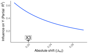
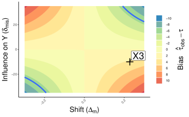
Figure 2: Sensitivity maps: On this figure $X_{3}$ is supposed to be a missing covariate. (Left) Regular sensitivity map showing how strong an key covariate would need to be to induce a bias of $\sim 6$ in function of the two sensitivity parameters $\Delta_{m}$ and partial $R^{2}$ when a covariate is totally unobserved. (Right) The exact same simulation data are represented, while using rather $\delta_{mis}$ than the partial $R^{2}$, and superimposing the heatmap of the bias which allows to reveal the general landscape along with the sign of the bias.

On Figure 2 we present a glimpse of the simulation result, to introduce the principle of the sensitivity map, with on the left the representation using $R^{2}$ and on the right a representation keeping the raw sensitivity parameters. In this plot, we consider the covariate $X_{3}$ to be missing, so that we represent what would be the bias if we missed $X_{3}$?, The associated sensitivity parameters are represented on each axis. In other word, the sensitivity map shows how strong an unobserved key covariate would need to be to induce a bias that would force to reconsider the conclusion of the study because the bias is above a certain threshold, that is represented by the blue line. For example in our simulation set-up, $X_{3}$ is below the threshold as illustrated on Figure 2. The threshold can be proposed by expert, and here we proposed the absolute difference between $\hat{\tau}_{n,m,obs}$ and the RCT estimate $\hat{\tau}_{1}$ as a natural quantity. In particular, we observe that keeping the sign of the sensitivity parameter allows to be even more confident on the direction of the bias.

3.3.4 Partially observed covariates: imputation

Another practically appealing solution is to impute the partially-observed covariate, based on the complete data set (whether it is the RCT or the observational one) following Procedure 4. We analyse theoretically in this section the bias of such procedure in Corollary 2, and show there is no gain in linearly imputing the partially-observed covariate.

To ease the mathematical analysis, we focus on a G-formula estimator based on oracles quantities: the best imputation function and the surface responses are assumed to be known. While these are not available in practice, they can be approached with consistent estimates of the imputation functions and the surface responses. The precise formulation s of our oracle estimates are given in Definition 2 and Definition 3.

Definition 2 (Oracle estimator when covariate is missing in the observational data set).

Assume that the RCT is complete and that the observational sample contains one missing covariate $X_{mis}$. We assume that we know

• the true response surface s $\mu_{1}$ and $\mu_{0}$

• the true linear relation between $X_{mis}$ as a function of $X_{obs}$.

Our oracle estimate $\hat{\tau}_{\text{\tiny G},\infty,m,imp}$ consists in applying the G-formula with the true response surfaces $\mu_{1}$ and $\mu_{0}$ (I) on the observational sample, in which the missing covariate has been imputed by the best (linear) function (II).

Definition 3 (Oracle estimator when covariate is missing in the RCT data set).

Assume that the observational sample is complete and that the RCT contains one missing covariate $X_{mis}$. We assume that we know

• the true linear relation between $X_{mis}$ as a function of $X_{obs}$, which leads to the optimal imputation $\hat{X}_{mis}$,

• the conditional expectations, $\mathbb{E}\left[Y(a)|X_{obs},\hat{X}_{mis},S=1\right]$, for $a\in\{0,1\}$.

Our oracle estimate $\hat{\tau}_{G,\infty,\infty,imp}$ consists in optimally imputing the missing variable $X_{mis}$ in the RCT (I). Then, the G-formula is applied to the observational sample, with the surface responses that have been perfectly fitted on the completed RCT sample.

Corollary 2 (Oracle bias of imputation in a Gaussian setting).

Assume that the CATE is linear (2) and that Assumption 7 holds. Let B be the following quantity:

$$B=\delta_{mis}\left(\mathbb{E}\left[X_{mis}\right]-\mathbb{E}\left[X_{mis}\mid S=1\right]-\Sigma_{j,obs}\Sigma_{obs,obs}^{-1}(\mathbb{E}\left[X_{obs}\right]-\mathbb{E}\left[X_{obs}\mid S=1\right])\right).$$

• Complete RCT. Assume that the RCT is complete and that the observational data set contains a missing covariate $X_{mis}$. Consider the oracle estimator $\hat{\tau}_{\text{\tiny G},\infty,m,imp}$ in Definition 2. Then,

  $$\tau-\lim\limits_{m\to\infty}\mathbb{E}[\hat{\tau}_{\text{\tiny G},\infty,m,imp}]=B$$

• Complete Observational. Assume that the observational data set is complete and that the RCT contains a missing covariate $X_{mis}$. Consider the oracle estimator $\hat{\tau}_{\text{\tiny G},\infty,\infty,imp}$ in Definition 3. Then,

  $$\tau-\mathbb{E}[\hat{\tau}_{\text{\tiny G},\infty,\infty,imp}]=B$$

Derivations are detailed in appendix (see Subsection C.2). Corollary 2 highlights that there is no gain in linearly imputing the missing covariate compared to dropping it. Simulations (Section F) show that the average bias of a finite-sample imputation procedure is similar to the bias of $\hat{\tau}_{\text{\tiny G},\infty,\infty,obs}$.

Model $X_{mis}$ a linear combination of $X_{obs}$ on the complete data set;

Impute the missing covariate with $\hat{X}_{mis}$ with the previous fitted model;

Compute $\hat{\tau}$ with the G-formula using the imputed data set $X_{obs}\cup\hat{X}_{mis}$;

return $\hat{\tau}$

Procedure 4 Linear imputation

3.3.5 Using a proxy variable in place of the missing covariate

Another solution is to use a so-called proxy variable. The impact of a proxy in the case of a linear model is documented in econometrics (Chen et al., 2005, 2007; Angrist and Pischke, 2008; Wooldridge, 2016). An example of a proxy variable is the height of children as a proxy for their age. Note that in this case, even if the age is present in one of the two datasets, only the children’s height is kept in for this method.

Here, we propose a framework to handle a missing key covariate with a proxy variable and estimate the bias reduction accounting for the additional noise brought by the proxy.

Assumption 8 (Proxy framework).

Assume that $X_{mis}\mathchoice{\mathrel{\hbox to0.0pt{$\displaystyle\perp$\hss}\mkern 2.0mu{\displaystyle\perp}}}{\mathrel{\hbox to0.0pt{$\textstyle\perp$\hss}\mkern 2.0mu{\textstyle\perp}}}{\mathrel{\hbox to0.0pt{$\scriptstyle\perp$\hss}\mkern 2.0mu{\scriptstyle\perp}}}{\mathrel{\hbox to0.0pt{$\scriptscriptstyle\perp$\hss}\mkern 2.0mu{\scriptscriptstyle\perp}}}X_{obs}$, and that there exist s a proxy variable $X_{prox}$ such that,

$$X_{prox}=X_{mis}+\eta$$

where $\mathbb{E}[\eta]=0$, $\operatorname{Var}[\eta]=\sigma_{prox}^{2}$, and $\operatorname{Cov}\left(\eta,X_{mis}\right)=0$. In addition we suppose that $\operatorname{Var}[X_{mis}]=\operatorname{Var}[X_{mis}\mid S=1]=\sigma_{mis}^{2}$.

Definition 4.

Let $\hat{\tau}_{\text{\tiny G},n,m,prox}$ be the G-formula estimator where $X_{mis}$ is substituted by $X_{prox}$ as detailed in assumption 8.

Lemma 1.

Assume that the generative linear model (2) holds, along with Assumption 7 and the proxy framework (8). Then the asymptotic bias of $\hat{\tau}_{\text{\tiny G},n,m,prox}$ is:

$$\lim\limits_{n,m\to\infty}\mathbb{E}[\hat{\tau}_{\text{\tiny G},n,m,prox}]-\tau=-\delta_{mis}\,\Delta_{m}\left(1-\frac{\sigma_{mis}^{2}}{\sigma_{mis}^{2}+\sigma_{prox}^{2}}\right)$$

We denote $\hat{\delta}_{prox}$ the estimated coefficient for $X_{prox}$ . Such an estimation can be obtained using a Robinson procedure when regressing $Y$ on the set $X_{obs}\cup X_{prox}$.

Corollary 3.

The asymptotic bias in lemma 1 can be estimated using the following expression:

$$\lim\limits_{n,m\to\infty}\mathbb{E}[\hat{\tau}_{\text{\tiny G},n,m,prox}]-\tau=-\hat{\delta}_{prox}\bigl{(}\mathbb{E}[X_{prox}]-\mathbb{E}[X_{prox}\mid S=1]\bigr{)}\frac{\sigma_{prox}^{2}}{\sigma_{mis}^{2}}$$

Proof s of Lemma 1 and Corollary 3 are detailed in Appendix (Proof C.3). Note that, as expected, the average bias reduction strongly depends on the quality of the proxy. In the limit case, if $\sigma_{prox}\sim 0$ so that the correlation between the proxy and the missing variable is one, then the bias is null. In general, if $\sigma_{prox}\gg\sigma_{mis}$ then the proxy variable does not diminish the bias. Finally, we propose a practical approach in Procedure 5. Note that it requires to have a range of possible $\sigma_{prox}$ values. We recommend to use the data set on which the proxy along with the partially-unobserved covariate are present, and to obtain an estimation of this quantity on this subset.

init :  $\sigma_{prox}:=[\dots]$ ;

  // Define a range for plausible $\sigma_{prox}$ values

if $X_{mis}$ is in RCT then

       init :  $\Delta_{mis}:=[\dots]$ ;

        // Define a range for plausible $\Delta_{mis}$ values

      

       Estimate $\delta_{mis}$ with the Robinson procedure (see Procedure 3 for details);

       Compute all possible bias es for the range of $\sigma_{prox}$ according to Lemma C.3.

      

else

       Estimate $\delta_{prox}$ with the Robinson procedure (see Procedure 3 for details);

       Estimate $\mathbb{E}[X_{prox}]$ and $\mathbb{E}[X_{prox}\mid S=1]$;

       Compute all possible bias for range of $\sigma_{prox}$ according to Corollary 3.

      

return Bias es’s range

Procedure 5 Proxy variable

4 Synthetic and semi-synthetic simulations

More information on simulation settings can be found in Appendix see Section F

4.1 Synthetic simulations

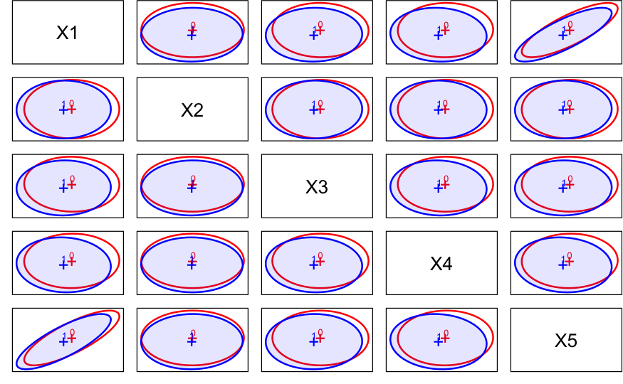
Figure 3: Variance-covariance preservation in the simulation set-up highlighted with pairwise covariance ellipses for one realization of the simulation (package heplots).

While results presented in Section 3 apply to any function $g$ (see (2)), we choose $g$ as a linear function to illustrate our findings. All simulations are available on github, and include non-linear forms for $g$.

Simulations parameters

We use a similar simulation framework as in Dong et al. (2020) and Colnet et al. (2020), where $5$ covariates are generated independently, except for $X_{1}$ and $X_{5}$ whose correlation is set at 0.8, except when explicitly mentioned . We simulate marginals as $X_{j}\sim\mathcal{N}(1,1)$ for all $j=1,\ldots,5$. The trial selection process is defined using a logistic regression model, such that:

$$\operatorname{logit}\left\{P(S=1\mid X)\right\}=\beta_{s,0}+\beta_{s,1}\,X_{1}+\dots+\beta_{s,5}\,X_{5}.$$ (7)

This selection process implies that the variance-covariance matrix in the RCT sample and in the target population may be different depending on the (absolute) value of the coefficients $\beta_{s}$. In our simulation set-up, the overall variance-covariance structure is kept identical as visualized on Figure 3. The outcome is generated according to a linear model, following Model 2, that is

$$Y(a)=\beta_{0}+\beta_{1}X_{1}+\dots+\beta_{5}X_{5}+a(\delta_{1}X_{1}+\dots+\delta_{5}X_{5})+\varepsilon\mbox{ with }\varepsilon\sim\mathcal{N}(0,1).$$ (8)

In this simulation, we set $\beta=(5,5,5,5,5)$, and other parameters as described in Table 3.

Covariates	$X_{1}$	$X_{2}$	$X_{3}$	$X_{4}$	$X_{5}$
Treatment effect modifier	Yes	Yes	Yes	No	No
Linked to trial inclusion	Yes	No	Yes	Yes	No
$\delta$	$\delta_{1}=30$	$\delta_{2}=30$	$\delta_{3}=-10$	$\delta_{4}=0$	$\delta_{5}=0$
$\beta_{s}$	$\beta_{s,1}=-0.4$	$\beta_{s,2}=0$	$\beta_{s,3}=-0.3$	$\beta_{s,4}=-0.3$	$\beta_{s,5}=0$
$.\mathchoice{\mathrel{\hbox to0.0pt{$\displaystyle\perp$\hss}\mkern 2.0mu{\displaystyle\perp}}}{\mathrel{\hbox to0.0pt{$\textstyle\perp$\hss}\mkern 2.0mu{\textstyle\perp}}}{\mathrel{\hbox to0.0pt{$\scriptstyle\perp$\hss}\mkern 2.0mu{\scriptstyle\perp}}}{\mathrel{\hbox to0.0pt{$\scriptscriptstyle\perp$\hss}\mkern 2.0mu{\scriptscriptstyle\perp}}}X_{1}$	-	$X_{2}\mathchoice{\mathrel{\hbox to0.0pt{$\displaystyle\perp$\hss}\mkern 2.0mu{\displaystyle\perp}}}{\mathrel{\hbox to0.0pt{$\textstyle\perp$\hss}\mkern 2.0mu{\textstyle\perp}}}{\mathrel{\hbox to0.0pt{$\scriptstyle\perp$\hss}\mkern 2.0mu{\scriptstyle\perp}}}{\mathrel{\hbox to0.0pt{$\scriptscriptstyle\perp$\hss}\mkern 2.0mu{\scriptscriptstyle\perp}}}X_{1}$	$X_{3}\mathchoice{\mathrel{\hbox to0.0pt{$\displaystyle\perp$\hss}\mkern 2.0mu{\displaystyle\perp}}}{\mathrel{\hbox to0.0pt{$\textstyle\perp$\hss}\mkern 2.0mu{\textstyle\perp}}}{\mathrel{\hbox to0.0pt{$\scriptstyle\perp$\hss}\mkern 2.0mu{\scriptstyle\perp}}}{\mathrel{\hbox to0.0pt{$\scriptscriptstyle\perp$\hss}\mkern 2.0mu{\scriptscriptstyle\perp}}}X_{1}$	$X_{4}\mathchoice{\mathrel{\hbox to0.0pt{$\displaystyle\perp$\hss}\mkern 2.0mu{\displaystyle\perp}}}{\mathrel{\hbox to0.0pt{$\textstyle\perp$\hss}\mkern 2.0mu{\textstyle\perp}}}{\mathrel{\hbox to0.0pt{$\scriptstyle\perp$\hss}\mkern 2.0mu{\scriptstyle\perp}}}{\mathrel{\hbox to0.0pt{$\scriptscriptstyle\perp$\hss}\mkern 2.0mu{\scriptscriptstyle\perp}}}X_{1}$	$X_{5}\not\mathchoice{\mathrel{\hbox to0.0pt{$\displaystyle\perp$\hss}\mkern 2.0mu{\displaystyle\perp}}}{\mathrel{\hbox to0.0pt{$\textstyle\perp$\hss}\mkern 2.0mu{\textstyle\perp}}}{\mathrel{\hbox to0.0pt{$\scriptstyle\perp$\hss}\mkern 2.0mu{\scriptstyle\perp}}}{\mathrel{\hbox to0.0pt{$\scriptscriptstyle\perp$\hss}\mkern 2.0mu{\scriptscriptstyle\perp}}}X_{1}$

Table 3: Simulations parameters.

First a sample of size $10,000$ is drawn from the covariate distribution. From this sample, the selection model (7) is applied which leads to an RCT sample of size $n\sim 2800$. Then, the treatment is generated according to a Bernoulli distribution with probability equal to $e_{1}=0.5$. Finally, the outcome is generated according to (8). The observational sample is obtained by drawing a new sample of size $m=10,000$ from the covariate distribution. In this setting, the ATE equals $\tau=\sum_{j=1}^{5}\delta_{j}\mathbb{E}[X_{j}]=\sum_{j=1}^{5}\delta_{j}=50$. Besides, the sample selection ($S=1$) in (7) is biased toward lower values of $X_{1}$ (and indirectly $X_{5}$), and higher values of $X_{3}$. This situation illustrate s a case where $\tau_{1}\neq\tau$. Empirically, we obtain $\tau_{1}\sim 44$.

Illustration of Theorem 1

Figure 4 presents results of a simulation with $100$ repetitions with no missing covariates (on the Figure see none), and the impact of missing covariate(s) when using the G-formula or the IPSW to generalize. The theoretical bias from Theorem 1 is also represented.

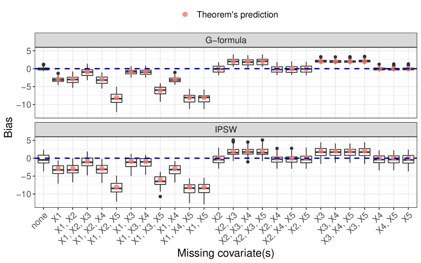
Figure 4: Illustration of Theorem 1: Simulation results for the linear model with missing covariate(s) when generalizing the treatment effect using the G-formula (Definition 1) or IPSW (see Definition 5 in appendix) estimator s on the set of observed covariates. Missing covariate are indicated on the x-axis. The theoretical bias (orange dot) is obtained from Theorem 1. Simulations are repeated 100 times.

The absence of covariates $X_{2},X_{4}$ and/or $X_{5}$ does not affect ATE generalization because these covariates are not simultaneously treatment effect modifiers and shifted (between the RCT sample and the target population). In addition, the sign s of the bias es depend on the sign s of the coefficient s associated to the missing variables, as highlighted by settings for which $X_{1}$ and $X_{3}$ are missing. As shown in Theorem 1, variables acting on $Y$ without being treatment effect modifiers and linked to trial inclusion can help to reduce the bias, if correlated to a (partially-) unobserved key covariate. This is stressed out in our experiment by comparing the settings for which $X_{1},X_{5}$ are missing and the one where only $X_{1}$ is missing.

A totally-unobserved covariate (from Section 3.3.1)

To illustrate this case, the missing covariate has to be supposed independent of all the others. For this paragraph we consider $X_{3}$. Then, according to Lemma 1, the two sensitivity parameters $\delta_{mis}$ and the shift $\Delta_{m}$ can be used to produce a sensitivity map for the bias on the transported ATE. The procedure 1 summarizes the different steps, and the sensitivity map’s output result was presented in Figure 2.

A missing covariate in the RCT (from Section 3.3.2)

In this case, we need to specify ranges of values for the two sensitivity parameters $\delta_{mis}$ and $\Delta_{m}$. The experimental protocol is designed such that all covariates are successively partially missing in the RCT. Because each missing variable implies a different landscape due to the dependence relation to other covariates (as stated in Theorem 1), each variable requires a different heatmap (except if covariates are all independent). Results are depicted in Figure 5. Figure 5 illustrates the benefit of Protocol 2 accounting for other correlated covariates , and compared to a protocol assuming independent covariates. Indeed, $X_{1}$ and $X_{2}$ are strong treatment effect modifiers (see Table 3, where $\delta_{1}=\delta_{2}$), but $X_{1}$ is correlated to other completely observed covariates, which allows to ”lower” the bias if $X_{1}$ is completely removed from the analysis compared to a similar covariate that would be independent of all other covariates. This is highlighted with a non-symetric bias landscape for $X_{1}$ on Figure 5. As a consequence, for a same value of $\delta_{mis}$ value, a guessed shift of $\Delta_{mis}=0.25$ allows to conclude on a lower bias on the map for $X_{1}$, while it would not be the case for covariate $X_{2}$ (which is completely independent).

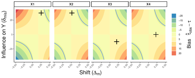
Figure 5: Simulations results when applying procedure 2: Heatmaps with a blue curve showing how strong an unobserved key covariate would need to be to induce a bias of $\tau_{1}-\tau\sim-6$ in function of the two sensitivity parameters $\Delta_{m}$ and $\delta_{mis}$ when a covariate is totally unobserved. Each heatmap illustrates a case where the covariate would be missing (indicated on the top of the map), given all other covariates. The cross indicate the coordinate of true sensitivity parameters, in adequation with the bias empirically observed in Figure 4. The bias landscape depends on the dependence of the covariate with other observed covariates, as illustrated with an asymmetric heatmap when $X_{1}$ is partially observed, due to the presence of $X_{5}$.

A missing covariate in the observational data (from Section 3.3.2)

In this case, we need to specify a range for the values of only one sensitivity parameter, namely $\mathbb{E}[X_{mis}]$ (see (5)). In our experimental protocol, we assume that $X_{1}$ is missing and apply Procedure 3 . Results are presented in Table 4.

Sensitivity parameter $\mathbb{E}[X_{mis}]$	0.8	0.9	1.0	1.1	1.2
Empirical average $\hat{\tau}_{\text{\tiny G},n,m,obs}$	44	47	50	53	56
Empirical standard deviation $\hat{\tau}_{G,n,m,obs}$	0.4	0.4	0.3	0.3	0.4

Table 4: Simulations results when applying procedure 3: Results of the simulation considering $X_{1}$ being partially observed in the RCT, and using the sensitivity method of Nguyen et al. (2017), but with a Robinson procedure to handle semi-parametric generative functions. When varying the sensitivity parameters, the estimated ATE is close to the true ATE ($\tau=50$) when the sensitivity parameter is closer to the true one ($\mathbb{E}[X_{mis}]=1$). The results are presented for 100 repetitions.

$\beta_{s,1}$	Averaged p-value
0	0.44
-0.2	0.37
-0.4	0.31
-0.6	0.14
-0.8	0.04
-1	0.012
-1.2	0.0001
-1.4	$1\cdot 10^{-9}$
-1.6	$1\cdot 10^{-10}$
-1.8	$3\cdot 10^{-15}$
-2	$1.4\cdot 10^{-23}$

Figure 6: Empirical link between the logistic regression coefficient for sampling bias $\beta_{s,1}$ and the p-value of a Box-M test. The average p-value is computed by repeating $50$ times the simulation. We recall that in Figure 4, $\beta_{s,1}:=-0.4$.

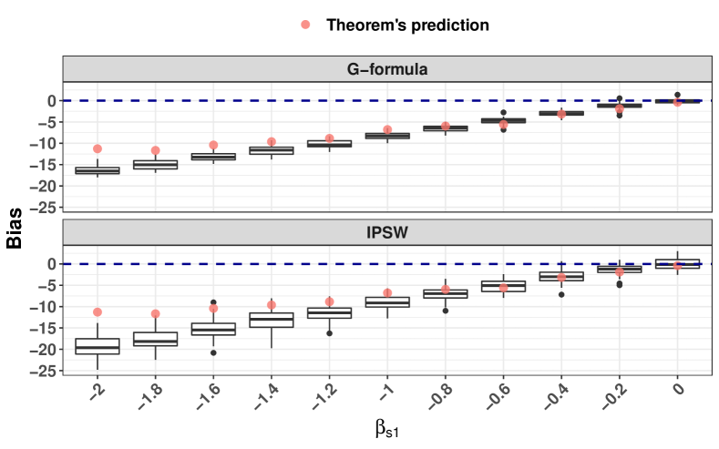
Figure 7: Impact of poor transportability of the variance-covariance matrix which is simulated with a decreasing coefficient $\beta_{s,1}$ , responsible of the covariate shift between the RCT sample and the observational sample. The lower $\beta_{s,1}$, the higher the absolute empirical bias (boxplots), and the higher the difference between the prediction s given by Theorem 1 (orange dots) compared to the effective empirical bias es (boxplots).

Simulations illustrating imputation (Corollary 2) and usage of a proxy (Lemma 1) are available in appendix, in Section F.

Violation of Assumption 7

To assess the impact of a lack of transportability of the variance -covariance matrix (Assumption 7) we propose to observe the effect of an increasing (in absolute value) coefficient involved in the sampling process (Equation 7). We observe that the bigger the coefficient, the bigger the deviations from the theory, as expected. To illustrate this phenomenon, we associate the logistic regression coefficient (the further away from the zero, the more Assumption 7 is unvalidated) to the p-value of a Box-M test assessing if the variance covariance matrix from the two sources are different. Empirically, the bias is still well estimated by procedures described in Section 3 even if the p-value is lower than $0.05$. Results are available on Figures 7 and 7.

4.2 A semi-synthetic simulation: the STAR experiment

The semi-synthetic experiment is a mean to evaluate the methods on (semi) real data where neither the data generation process nor the distribution of the covariates are under control.

4.2.1 Simulation details

We use the data from a randomized controlled trial, the Tennessee Student/Teacher Achievement Ratio (STAR) study. This RCT is a pioneering randomized study from the domain of education (Angrist and Pischke, 2008), started in 1985, and designed to estimate the effects of smaller classes in primary school, on the children’s grades. This experiment showed a strong payoff to smaller classes (Finn and Achilles, 1990). In addition, the effect has been shown to be heterogeneous (Krueger, 1999), where class size s have a larger effect for minority students and those on subsidized lunch. For our purposes, we focus on the same subgroup of children, same treatment (small versus regular classes), and same outcome (average of all grades at the end) as in Kallus et al. (2018).

4 218 children are concerned by the treatment randomization, with treatment assignment at first grade only. On the whole data, we estimated an average treatment effect of 12.80 additional points on the grades (95% CI [10.41-15.2]) with the difference-in-means estimator. We consider this estimate as the ground truth $\tau$ as it is the global RCT. Then, we generate a random sample of 500 children to serve as the observational study. From the rest of the data, we sample a biased RCT according to a logistic regression that defines probability for each class to be selected in the RCT, and using only the variable g1surban informing on the neighborhood of the school , which can be considered as a proxy for the socioeconomic status. The final selection is performed using a Bernoulli procedure, which leads to 563 children in the RCT. The resulting RCT is such that $\hat{\tau}_{1}$ is 4.85 (95% CI [-2.07-11.78]) which is underestimated. This is due to the fact that that the selection is performed toward children that benefit less from the class size reduction according to previous studies (Finn and Achilles, 1990; Krueger, 1999; Kallus et al., 2018). When generalizing the ATE with the G-formula on the full set of covariates, estimating the nuisance components with a linear model, and estimating the confidence intervals with a stratified bootstrap (1000 repetitions), the target population ATE is recovered with an estimate of 13.05 (95% CI [5.07-22.11]) Not including the covariate on which the selection is performed (g1surban) leads to a biased generalized ATE of 5.87 (95% CI [-1.47-12.82]). These results are represented on Figure 8, along with AIPSW estimates. The IPSW is not represented due to a too large variance.

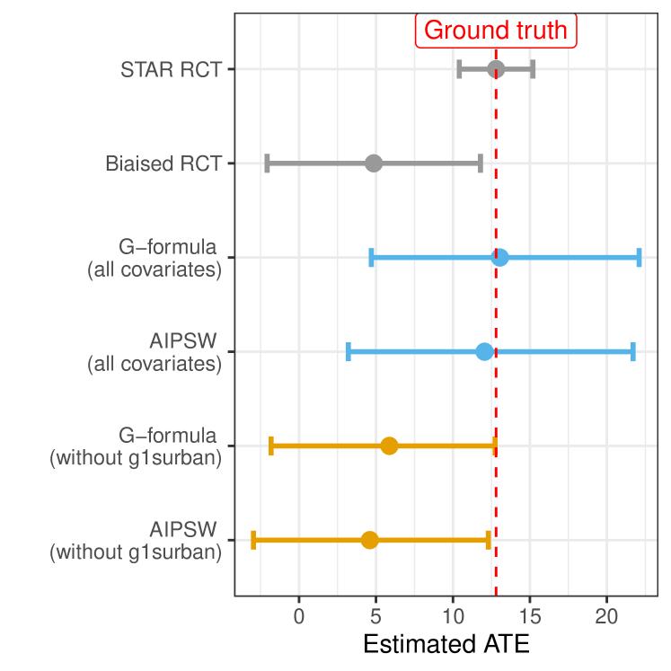
Figure 8: Simulated STAR data: True target population ATE estimation using all the STAR’s RCT data is represented (difference-in-means). This is highlighted with a red dashed line to represent the ground truth. The ATE estimate of a biased RCT (difference-in-means) is also represented showing a lower treatment effect due to a covariate shift along the covariate g1surban. Two estimators are used for the generalization, the G-formula (Definition 1) and the AIPSW (Definition 6); both relying on linear or logistic models for the nuisance components. The generalized ATE is either estimated with all covariates (blue) or with all covariates except g1surban (orange). The confidence intervals are estimated with a stratified bootstrap (1000 repetitions). Similar results are obtained when nuisance components are estimated with random forest.

4.2.2 Application of the sensitivity methods

We now successively consider two different missing covariate patterns to apply the methods from Section 3.3.2.

Considering g1surban is missing in the observational study

Nguyen et al. (2017)’s method (recalled in Section 3.3.2) can be applied, if we are given a set of plausible values for $\mathbb{E}[\text{g1surban}]$. Specifying the following range $\left]2.1,2.7\right[\$ (containing the true value for $\mathbb{E}[\text{g1surban}]$) leads to a range for the generalized ATE of $\left]9.5,16.7\right[.$ Recalling that the ground truth is 12.80 (95% CI[10.41-15.2]), the estimated range has a good overlap with the ground truth. In other words, with this specification of the range, a user would correctly conclude that without this key variable, the generalized ATE is probably underestimated.

Considering g1surban is missing in the RCT

Figure 9 illustrates the method when the missing covariate is in the RCT data set (see Procedure 2). This method relies on Assumption 7, which we test with a Box M-test on $\Sigma$ (though in practice such a test could only be performed on $\Sigma_{obs,obs}$). Including only numerical covariates would reject the null hypothesis ($p-value=0.034$). Note that beyond violating Assumption 7, some variables are categorical (eg race and gender). Further discussions about violation of this assumption are available in appendix (Section G).

In this application, applying recommendations from Section 3.3.2 (see paragraph entitled Data-driven approach to determine sensitivity parameter) allow us to get $\delta_{\texttt{g1surban}}\sim 11$. We consider that the shift is correctly given by domain expert, and so the true shift is taken with uncertainty corresponding to the 95% confidence interval of a difference in mean. Finally, Figure 9 allows to conclude on a negative bias, that is $\mathbb{E}[\hat{\tau}_{n,m,obs}]\leq\tau$. Note that our method underestimate a bit the true bias, with an estimated bias of $-6.4$ when the true bias is $-7.08$, delimited with the continue red curve on the top right.

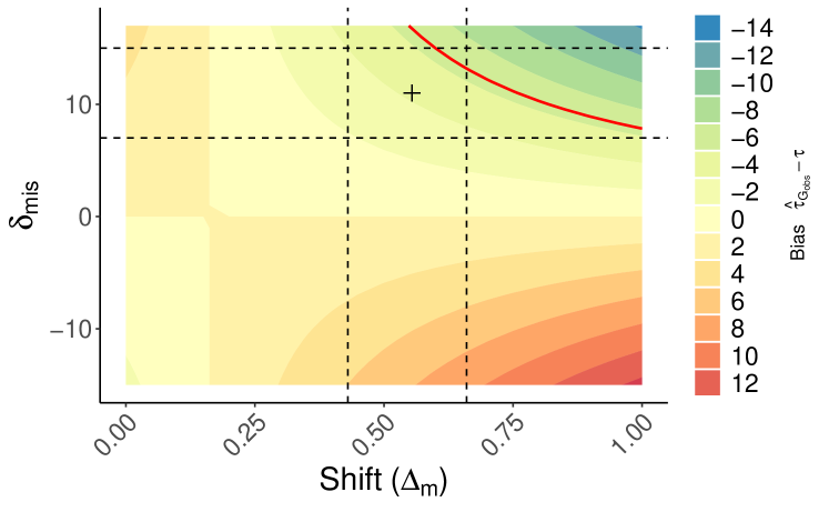
Figure 9: Sensitivity analysis of STAR data: considering the covariate g1surban is missing in the RCT. The black cross indicates the point estimate value for the bias would an expert have the true sensitivity values ($-6.4$) and the true bias value is represented with the red line ($-7.08$). Dashed lines corresponds to the 95% confidence intervals around the estimated sensitivity parameters.

5 Application on critical care data

A motivating application of our work is the generalization to a French target population – represented by the Traumabase registry – of the CRASH-3 trial (CRASH-3, 2019), evaluating Tranexamic Acide (TXA) to prevent death from Traumatic Brain Injury (TBI).

CRASH-3

A total of 175 hospitals in 29 different countries participated to the randomized and placebo-controlled trial, called CRASH-3 (Dewan et al., 2012), where adults with TBI suffering from intracranial bleeding were randomly administrated TXA (CRASH-3, 2019). The inclusion criteria of the trial are patients with a Glasgow Coma Scale (GCS) score of 12 or lower or any intracranial bleeding on CT scan, and no major extracranial bleeding. The outcome we consider in this application is the Disability Rating Scale (DRS) after 28 days of injury in patients treated within 3 hours of injury. Such an index is a composite ordinal indicator ranging from 0 to 29, the higher the value, the stronger the disability. This outcome can be considered as a secondary outcome.This outcome has some drawbacks in the sense that TXA diminishes the probability to die from TBI, and therefore may increase the number of high DRS values (Brenner et al., 2018). Therefore, to avoid a censoring or truncation due to death, we keep all individuals and set the DRS score of deceased ones to 30. The difference-in-means estimator gives an ATE of -0.29 with [95% CI -0.80 0.21]), therefore not giving a significant evidence of an effect of TXA on DRS.

Traumabase

To improve decisions and patient care in emergency departments, the Traumabase group, comprising 23 French Trauma centers, collects detailed clinical data from the scene of the accident to the release from the hospital. The resulting database, called the Traumabase, comprises 23,000 trauma admissions to date, and is continually updated. In this application, we consider only the patients suffering from TBI, along with considering an imputed database. The Traumabase comprises a large number of missing values, this is why we used a multiple imputation via chained equations (MICE) (van Buuren, 2018) prior to applying our methodology.

Predicting the treatment effect on the Traumabase data

We want to generalize the treatment effect to the French patients - represented by the Traumabase data base. Six covariates are present at baseline, with age, sex, time since injury, systolic blood pressure, Glasgow Coma Scale score (GCS), and pupil reaction. Sex is not considered in the final sensitivity analysis as a non-continuous covariate, and pupil reaction is considered as continuous ranging from 0 to 2. However an important treatment effect modifier is missing, that is the time between treatment and the trauma. For example, Mansukhani et al. (2020) reveal a 10% reduction in treatment effectiveness for every 20-min increase in time to treatment (TTT). In addition TTT is probably shifted between the two populations. Therefore this covariate breaks assumption 4 (ignorability on trial participation), and we propose to apply the methods developed in Section 3.

Sensitivity analysis

The concatenated data set with the RCT and observational data contains 12 496 observations (with $n=8\,977$ and $m=7\,743$). Considering a totally -missing covariate, we apply Procedure 1. We assume that time-to-treatment (TTT) is independent of all other variables, for example the ones related to the patient baseline characteristics (e.g. age) or to the severity of the trauma (e.g. the Glasgow score). Clinicians support this assumption as the time to receive the treatment depends on the time for the rescuers to come to the accident area, and not on the other patient characteristics. We first estimate the target population treatment effect with the set of observed variables and the G-formula estimator, leading to an estimated ATE $\hat{\tau}_{n,m,obs}$ of -0.08 (95% CI [-0.50 0.44]). The nuisance parameters are estimated using random forests, and the confidence interval with non-parametric stratified bootstrap. As the omission of the TTT variable could affect this conclusion, the sensitivity analysis gives insights on the potential bias.

We apply the method relative to a completely missing covariate (Section 3.3.1). A common practice in sensitivity analysis is to use observed covariates as benchmark to guess the impact of an unobserved covariates. For example, the Glasgow score is also suspected to be a treatment effect modifier and is shifted between the two populations. We place it on a sensitivity map (Figure 11) along with the true corresponding values for $\delta_{\text{\tiny glasgow}}$ and $\Delta_{\text{\tiny glasgow}}$. As the Traumabase contain more individuals with a higher Glasgow score, a positive shift is reported. In addition, the higher the Glasgow score the higher the effect (low DRS), so that $\delta_{\text{\tiny glasgow}}<0$. Finally, removing the Glasgow score from the analysis would lead to $\hat{\tau}_{obs,n,m}>\tau$. The sensitivity map does not allow to conclude that this bias is big enough compared to the confidence intervals previously mentioned for $\hat{\tau}_{obs,n,m}$. Is the TTT a stronger or more shifted covariate than the Glasgow score? Previous publications have suggested a huge impact of TTT, and therefore one could expect a bigger impact on the bias. On Figure 11 we represent a sensitivity map for TTT that could be drawn by domain experts. Here, sensitivity parameters are guessed. For example, one can suspect that treatment is given on average 20 minutes earlier in the Traumabase (for example interviewing nurses and doctors in Trauma centers), and the coefficient $\delta_{\text{\tiny TTT}}$ is inferred from a previous work on TXA. On Figure 11, one can see that not observing TTT has a bigger impact on the bias than not observing the Glasgow score (almost 10 times bigger), suggesting another conclusion: a positive and significant effect of TXA on the Traumabase population, if the sensitivity parameters are correctly guessed. Also, as soon as there is a risk of a treatment given later than in the CRASH3 trial, this sensitivity map would help raising an alarm on a negative effect on the Traumabase population.

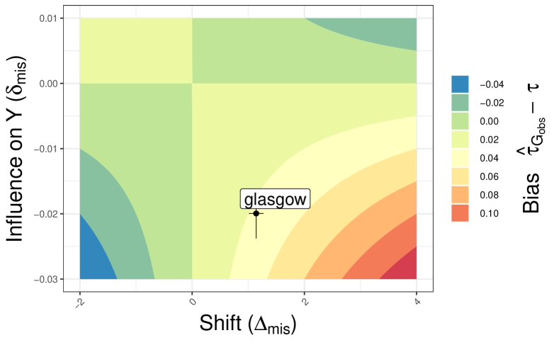
Figure 10: Sensitivity map if the Glasgow score covariate was missing: the true corresponding values for $\delta_{\text{\tiny glasgow}}$ and $\Delta_{\text{\tiny glasgow}}$ are computed with respectively a Robinson proceadure and a mean difference. Intervals correspond to 95% confidence intervals.

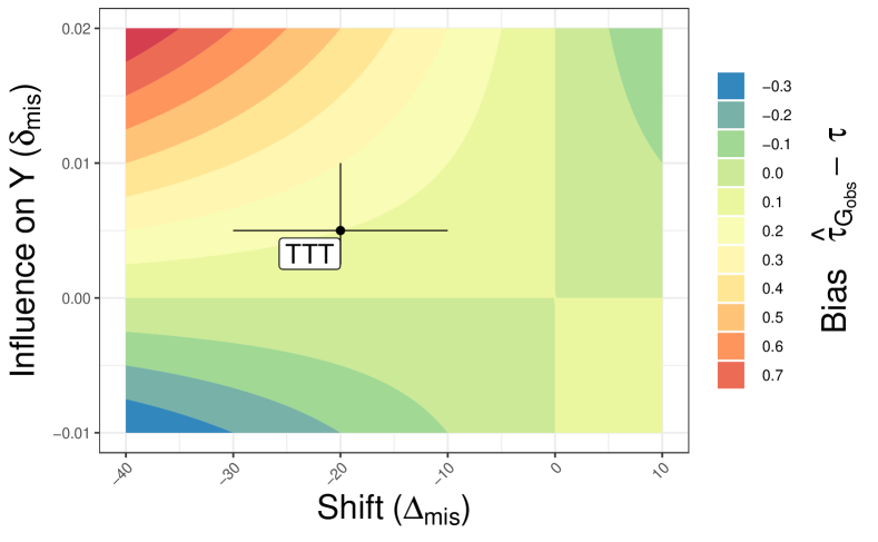
Figure 11: Sensitivity map for TTT: Intervals represent plausible parameters range, with a treatment given on average 10 to 30 minutes earlier in the Traumabase, and an heterogeneous coefficient inspired from Mansukhani et al. (2020).

Conclusion

In this work, we have studied sensitivity analyses for causal-effect generalization to assess the impact of a partially-unobserved confounder (either in the RCT or in the observational data set) on the ATE estimation. In particular:

1. To go beyond the common requirement that the unobserved confounder is independent from the observed covariates, we instead assume that their covariance is transported (Assumption 7). Our simulation study (4) shows that even with a slightly deformed covariance, the proposed sensitivity analysis procedure give s useful estimates of the bias.

2. Leveraging the high interpretability of our sensitivity parameter, our framework concludes on the sign of the estimated bias. This sign is important as accepting a treatment effect highly depends on the direction of the generalization shift. We integrate the above methods into the existing sensitivity map visualization, using a heatmap to represent the sign of the estimated bias.

3. Our procedures use a sensitivity parameter with a direct interpretation: the shift in expectation $\Delta_{m}$ of the missing covariate between the RCT and the observational data. We hope that this will ease practical applications of sensitivity analyses by domain experts.

Our proposal inherits limitations from the more standard sensitivity analysis methods with observational data, namely the semi-parametric assumption of the outcome model along with an hypothesis on covariate structures (Gaussian inputs). Therefore, future extensions of this work could explore ways to relax either the parametric assumption or the distributional assumption to support more robust sensitivity analyses. Another possible extension to a missing binary covariate could be deduced from this work, in the case where this covariate is independent of the others in both population s.

Supplementary information

Appendix A Estimators of the target population ATE

In this section, we grant assumptions presented in Section 2.1 and study the asymptotic behavior – and in particular the $L^{1}$-consistency – of three estimators: the G-formula, the IPSW, and the AIPSW.

A.1 G-formula

The G-formula procedure and its consistency assumption are detailed in the core text, see Section 3, and in particular Definition 1 and Assumption 6. Here, we present the Theorem for consistency.

Theorem 2 (G-formula consistency).

Consider the G-formula estimator in Definition 1 along with Assumptions 1, 2, 3, 4, 5 (identifiability), and Assumption 6 (consistency), then the G-formula estimator converges toward $\tau$ in $L^{1}$ norm,

$$\hat{\tau}_{\text{{\tiny G}},n,m}\underset{n,m\to\infty}{\overset{L^{1}}{\longrightarrow}}\tau.$$

A.2 IPSW

Another approach, called Inverse Propensity Weighting Score (IPSW), consists in weighting the RCT sample so that is ressembles the target population distribution.

Definition 5 (Inverse Propensity Weighting Score - IPSW - Stuart et al. (2011); Buchanan et al. (2018)).

The IPSW estimator is denoted $\hat{\tau}_{\mathrm{IPSW},n,m}$, and defined as

$$\hat{\tau}_{\mathrm{IPSW},n,m}=\frac{1}{n}\sum_{i=1}^{n}\frac{n}{m}\frac{Y_{i}}{\hat{\alpha}_{n,m}(X_{i})}\left(\frac{A_{i}}{e_{1}(X_{i})}-\frac{1-A_{i}}{1-e_{1}(X_{i})}\right)\,,$$ (9)

where $\hat{\alpha}_{n,m}$ is an estimate of the odd ratio of the indicatrix of being in the RCT:

$$\alpha(x)=\frac{P(i\in\mathcal{R}\mid\exists i\in\mathcal{R}\cup\mathcal{O},X_{i}=x)}{P(i\in\mathcal{O}\mid\exists i\in\mathcal{R}\cup\mathcal{O},X_{i}=x)}.$$

This intermediary quantity to estimate, $\alpha(.)$, is called a nuisance component.

Similarly to the G-formula, we introduce here an assumption on the behavior of the nuisance component $\alpha$ to carry out the mathematical analysis of the IPSW.

Assumption 9 (Consistency assumptions - IPSW).

Denoting by $\frac{n}{m\hat{\alpha}_{n,m}(x)}$ the estimated weights on the set of observed covariates $X$, the following conditions hold,

• (H1-IPSW) $\sup_{x\in\mathcal{X}}|\frac{n}{m\hat{\alpha}_{n,m}(x)}-\frac{f_{X}(x)}{f_{X\mid S=1}(x)}|=\epsilon_{n,m}\stackrel{{\scriptstyle a.s.}}{{\longrightarrow}}0\text{ , when }n,m\rightarrow\infty$,

• (H2-IPSW) for all $n,m$ large enough $\mathbb{E}[\varepsilon_{n,m}^{2}]$ exists and $\mathbb{E}[\varepsilon_{n,m}^{2}]\stackrel{{\scriptstyle a.s.}}{{\longrightarrow}}0\text{ , when }n,m\rightarrow\infty$,

• (H3-IPSW) $Y$ is square integrable.

Theorem 3 (IPSW consistency).

Consider the IPSW estimator in Definition 5 along with Assumptions 1, 2, 3, 4, 5 (identifiability), and Assumption 9 (consistency). Then, $\hat{\tau}_{\text{\tiny IPSW},n,m}$ converges toward $\tau$ in $L^{1}$ norm,

$$\hat{\tau}_{\text{{\tiny IPSW}},n,m}\underset{n,m\to\infty}{\overset{L^{1}}{\longrightarrow}}\tau.$$

Theorem 3 establish es the consistency of IPSW in a more general framework than that of Cole and Stuart (2010); Stuart et al. (2011); Bareinboim and Pearl (2013); Buchanan et al. (2018); Egami and Hartman (2021), assuming neither oracle estimator, nor parametric assumptions on $\alpha(.)$.

A.3 AIPSW

The model for the expectation of the outcomes among randomized individuals (used in the G-estimator in Definition 1) and the model for the probability of trial participation (used in IPSW estimator in Definition 5) can be combined to form an Augmented IPSW estimator (AIPSW) that has a doubly robust statistical property.

Definition 6 (Augmented IPSW - AIPSW - Dahabreh et al. (2019)).

The AIPSW estimator is denoted $\hat{\tau}_{\text{\tiny AIPSW},n,m}$, and defined as

$$\begin{split}\hat{\tau}_{\text{\tiny AIPSW},n,m}=\frac{1}{n}\sum_{i=1}^{n}\frac{n}{m\,\hat{\alpha}_{n,m}(X_{i})}\left[\frac{A_{i}\left(Y_{i}-\hat{\mu}_{1,n}(X_{i})\right)}{e_{1}(X_{i})}-\frac{(1-A_{i})\left(Y_{i}-\hat{\mu}_{0,n}(X_{i})\right)}{1-e_{1}(X_{i})}\right]\\ +\frac{1}{m}\sum_{i=n+1}^{m+n}\left(\hat{\mu}_{1,n}(X_{i})-\hat{\mu}_{0,n}(X_{i})\right).\end{split}$$

Recently, it has been shown that the AIPSW estimator can be derived from the influence function of the parameter $\tau$ (see Dahabreh et al., 2019). Under additional conditions on the rate of convergence of the nuisance parameters, it is possible to obtain asymptotic normality results. As in this work we only require $L^{1}$-consistency for the sensitivity analysis to hold, we therefore do not detail asymptotic normality conditions.

To prove AIPSW consistency, we make the following assumptions on the nuisance parameters.

Assumption 10 (Consistency assumptions - AIPSW).

The nuisance parameters are bounded, and more particularly

• (H1-AIPSW) There exists a function $\alpha_{0}$ bounded from above and below (from zero), satisfying

  $$\lim\limits_{m,n\to\infty}\sup_{x\in\mathcal{X}}\biggr{|}\frac{n}{m\hat{\alpha}_{n,m}(x)}-\frac{1}{\alpha_{0}(x)}\biggl{|}=0,$$

• (H2-AIPSW) There exist two bounded functions $\xi_{1},\xi_{0}:\mathcal{X}\to\mathbb{R}$, such that $\forall a\in\{0,1\},$

  $$\lim\limits_{n\rightarrow+\infty}\sup_{x\in\mathcal{X}}|\xi_{a}(x)-\hat{\mu}_{a,n}(x)|=0.$$

Theorem 4 (AIPSW consistency).

Consider the AIPSW estimator in Definition 6, along with Assumptions 1, 2, 3, 4, 5 hold (identifiability), and Assumption 10 (consistency). Considering that estimated surface responses $\hat{\mu}_{a,n}(.)$ where $a\in\{0,1\}$ are obtained following a cross-fitting estimation, then if Assumption 6 or Assumption 9 also holds then, $\hat{\tau}_{\text{\tiny AIPSW},n,m}$ converges toward $\tau$ in $L^{1}$ norm,

$$\hat{\tau}_{\text{{\tiny AIPSW}},n,m}\underset{n,m\to\infty}{\overset{L^{1}}{\longrightarrow}}\tau.$$

Appendix B $L^{1}$-convergence of G-formula, IPSW, and AIPSW

This appendix contains the proofs of theorems given in Section A. We recall that this work completes and details existing theoretical work performed by Buchanan et al. (2018) on IPSW (but focused on a so called nested-trial design and assuming parametric model for the weights) and from Dahabreh et al. (2020) developing results within the semi-parametric theory.

B.1 $L^{1}$-convergence of G-formula

This section contains the proof of Theorem 2, which assumes Assumption 6. For the state of clarity, we recall here Assumption 6. Denoting $\hat{\mu}_{0,n}(.)$ and $\hat{\mu}_{1,n}(.)$ estimators of $\mu_{0}(.)$ and $\mu_{1}(.)$ respectively, and $\mathcal{D}_{n}$ the RCT sample, so that

• (H1-G) For $a\in\{0,1\}$, $\mathbb{E}\left[|\hat{\mu}_{a,n}(X)-\mu_{a}(X)|\mid\mathcal{D}_{n}\right]\stackrel{{\scriptstyle p}}{{\rightarrow}}0$ when $n\rightarrow\infty$,

• (H2-G) For $a\in\{0,1\}$, there exist $C_{1},N_{1}$ so that for all $n\geqslant N_{1}$, almost surely, $\mathbb{E}[\hat{\mu}_{a,n}^{2}(X)\mid\mathcal{D}_{n}]\leqslant C_{1}$.

Proof of Theorem 2.

In this proof, we largely rely on a oracle estimator $\hat{\tau}_{\text{\tiny G},\infty,m}^{*}$ (built with the true response surfaces), defined as

$$\hat{\tau}_{\text{\tiny G},\infty,m}^{*}=\frac{1}{m}\sum_{i=n+1}^{n+m}\mu_{1}(X_{i})-\mu_{0}(X_{i}).$$

The central idea of this proof is to compare the actual G-formula $\hat{\tau}_{\text{\tiny G},n,m}$ - on which the nuisance parameters are estimated on the RCT data - with the oracle.

$L^{1}$-convergence of the surface responses

For the proof, we will require that the estimated surface responses $\hat{\mu}_{1,n}(.)$ and $\hat{\mu}_{0,n}(.)$ converge toward the true ones in $L^{1}$. This is implied by assumptions (H1-G) and (H2-G). Indeed, for all $n>0$ and all $a\in\{0,1\}$, thanks to the triangle inequality and linearity of expectation, we have

$$\mathbb{E}\left[\left|\hat{\mu}_{a,n}(X)-\mu_{a}(X)\right|\mid\mathcal{D}_{n}\right] \leq\mathbb{E}\left[\left|\hat{\mu}_{a,n}(X)\right|\mid\mathcal{D}_{n}\right]+\mathbb{E}\left[\left|\mu_{a}(X)\right|\mid\mathcal{D}_{n}\right]$$

$$=\underbrace{\mathbb{E}\left[\left|\hat{\mu}_{a,n}(X)\right|\mid\mathcal{D}_{n}\right]}_{\textrm{(*)}}+\underbrace{\mathbb{E}\left[\left|\mu_{a}(X)\right|\right]}_{\textrm{(**)}}.$$

First, note that the quantity (*) is upper bounded thanks to assumption (H2-G), using Jensen’s inequality. Also note that the quantity (**) is upper bounded because the potential outcomes are integrables, that is $\mathbb{E}[|Y(1)|]$ and $\mathbb{E}[|Y(0)|]$ exist (see Section 2.1).

Therefore $\mathbb{E}\left[\left|\hat{\mu}_{a,n}(X)-\mu_{a}(X)\right|\mid\mathcal{D}_{n}\right]$ is upper bounded. Consequently, using (H2-G) and a generalization of the dominated convergence theorem, one has

$$\mathbb{E}\left[\left|\hat{\mu}_{a,n}(X)-\mu_{a}(X)\right|\right]=\mathbb{E}\left[\mathbb{E}\left[\left|\hat{\mu}_{a,n}(X)-\mu_{a}(X)\right|\mid\mathcal{D}_{n}\right]\right]\underset{n\to\infty}{\longrightarrow}0,$$

which implies

$$\forall a\in\{0,1\},\,\hat{\mu}_{a,n}(X)\underset{n\to\infty}{\overset{L^{1}}{\longrightarrow}}\mu_{a}(X).$$

$L^{1}$-convergence of $\hat{\tau}_{\text{\tiny G},n,m}$ toward $\tau$

For all $m,n>0$,

$$\hat{\tau}_{\text{\tiny G},n,m}-\hat{\tau}_{\text{\tiny G},\infty,m}^{*} =\frac{1}{m}\sum_{i=n+1}^{n+m}\left(\hat{\mu}_{1,n}(X_{i})-\hat{\mu}_{0,n}(X_{i})\right)-\left(\mu_{1}(X_{i})-\mu_{0}(X_{i})\right)$$

$$=\frac{1}{m}\sum_{i=n+1}^{n+m}\left(\hat{\mu}_{1,n}(X_{i})-\mu_{1}(X_{i})\right)-\left(\hat{\mu}_{0,n}(X_{i})-\mu_{0}(X_{i})\right).$$

Therefore, taking the expectation of the absolute value on both side, and using the triangle inequality and the fact that observations are iid,

$$\mathbb{E}\left[\left|\hat{\tau}_{\text{\tiny G},n,m}-\hat{\tau}_{\text{\tiny G},\infty,m}^{*}\right|\right] =\mathbb{E}\left[\left|\frac{1}{m}\sum_{i=n+1}^{n+m}\left(\hat{\mu}_{1,n}(X_{i})-\mu_{1}(X_{i})\right)-\left(\hat{\mu}_{0,n}(X_{i})-\mu_{0}(X_{i})\right)\right|\right]$$

$$\leq\mathbb{E}\left[\left|\hat{\mu}_{1,n}(X)-\mu_{1}(X)\right|\right]+\mathbb{E}\left[\left|\hat{\mu}_{0,n}(X)-\mu_{0}(X)\right|\right].$$

Note that this last inequality can be obtained because different observations are used to $(i)$ build the estimated surface responses $\hat{\mu}_{a,n}$ (for $a\in\{0,1\}$) and $(ii)$ to evaluate these estimators. Indeed, the proof would be much more complex if the sum was taken over the $n$ observations used to fit the models. Due to the $L^{1}$-convergence of each of the surface response when $n\rightarrow\infty$ (see the first part of the proof), we have

$$\lim_{n\to\infty}\mathbb{E}\left[\left|\hat{\tau}_{\text{\tiny G},n,m}-\hat{\tau}_{\text{\tiny G},\infty,m}^{*}\right|\right]=0.$$

In other words,

$$\forall m,\,\hat{\tau}_{\text{{\tiny G}},n,m}\underset{n\to\infty}{\overset{L^{1}}{\longrightarrow}}\hat{\tau}_{\text{\tiny G},\infty,m}^{*}.$$ (10)

This equality is true for any $m$, and intuitively can be understood as the fitted response surfaces $\hat{\mu}_{a,n}(.)$ can be very close to the true ones as soon as $n$ is large enough. Then, the G-formula estimator, no matter the size of the observational data set, is close to the oracle one in $L^{1}$. Hence one can deduce a result on the difference between $\tau$ and the G-formula,

$$\mathbb{E}\left[\left|\hat{\tau}_{\text{\tiny G},n,m}-\tau\right|\right] \leq\mathbb{E}\left[\left|\hat{\tau}_{\text{\tiny G},n,m}-\hat{\tau}_{\text{\tiny G},\infty,m}^{*}\right|\right]+\mathbb{E}\left[\left|\hat{\tau}_{\text{\tiny G},\infty,m}^{*}-\tau\right|\right].$$

According to the weak law of large number, we have

$$\hat{\tau}_{\text{\tiny G},\infty,m}^{*}\underset{m\to\infty}{\overset{L^{1}}{\longrightarrow}}\tau$$

Combining this result with equation (10), we have

$$\hat{\tau}_{\text{{\tiny G}},n,m}\underset{n,m\to\infty}{\overset{L^{1}}{\longrightarrow}}\tau,$$

which concludes the proof.

∎

B.2 $L^{1}$-convergence of IPSW

This section provides the proof of Theorem 3, and for the sake of clarity, we recall Assumption 9. Denoting $\frac{n}{m\hat{\alpha}_{n,m}(x)}$, the estimated weights on the set of covariates $X$, the following conditions hold,

• (H1-IPSW) $\sup_{x\in\mathcal{X}}|\frac{n}{m\hat{\alpha}_{n,m}(x)}-\frac{f_{X}(x)}{f_{X\mid S=1}(x)}|=\varepsilon_{n,m}\stackrel{{\scriptstyle a.s.}}{{\longrightarrow}}0\text{ , when }n,m\rightarrow\infty$,

• (H2-IPSW) we have for all $n,m$ large enough $\mathbb{E}[\varepsilon_{n,m}^{2}]$ exists and $\mathbb{E}[\varepsilon_{n,m}^{2}]\stackrel{{\scriptstyle a.s.}}{{\longrightarrow}}0\text{ , when }n,m\rightarrow\infty$,

• (H3-IPSW) $Y$ is square integrable.

Proof of Theorem 3.

First, we consider an oracle estimator $\hat{\tau}_{\text{\tiny IPSW},n}^{*}$ that is based on the true ratio $\frac{f_{X}(x)}{f_{X\mid S=1}(x)}$, that is

$$\hat{\tau}_{\text{\tiny IPSW},n}^{*}=\frac{1}{n}\sum_{i=1}^{n}Y_{i}\frac{f_{X}(X_{i})}{f_{X\mid S=1}(X_{i})}\left(\frac{A_{i}}{e_{1}(X_{i})}-\frac{1-A_{i}}{1-e_{1}(X_{i})}\right).$$

Note that Egami and Hartman (2021) also consider such an estimator and document its consistency (see their appendix). Indeed, assuming the finite variance of $Y$, the strong law of large numbers (also called Kolmogorov’s law) allows us to state that:

$$\hat{\tau}_{\text{\tiny IPSW},n}^{*}\stackrel{{\scriptstyle a.s.}}{{\longrightarrow}}\mathbb{E}\Big{[}Y\frac{f_{X}(X)}{f_{X\mid S=1}(X)}\Big{(}\frac{A}{e_{1}(X)}-\frac{1-A}{1-e_{1}(X)}\Big{)}\mid S=1\Big{]}=\tau,\quad\textrm{as}~{}n\to\infty.$$ (11)

Now, we need to prove that this result also holds for the estimate $\hat{\tau}_{\text{\tiny IPSW},n,m}$ where the weights are estimated from the data. To this aim, we first use the triangle inequality comparing $\hat{\tau}_{\text{\tiny IPSW},n,m}$ with the oracle IPSW:

$$\Big{|}\hat{\tau}_{\text{\tiny IPSW},n,m}-\hat{\tau}_{\text{\tiny IPSW},n}^{*}\Big{|} =\Big{|}\frac{1}{n}\sum_{i=1}^{n}\left(\frac{A_{i}Y_{i}}{e_{1}(X_{i})}-\frac{(1-A_{i})Y_{i}}{1-e_{1}(X_{i})}\right)\left(\frac{n}{\hat{\alpha}_{n,m}(X_{i})m}-\frac{f_{X}(X_{i})}{f_{X\mid S=1}(X_{i})}\right)\Big{|}$$

$$\leq\frac{1}{n}\sum_{i=1}^{n}\Big{|}\left(\frac{A_{i}Y_{i}}{e_{1}(X_{i})}-\frac{(1-A_{i})Y_{i}}{1-e_{1}(X_{i})}\right)\left(\frac{n}{\hat{\alpha}_{n,m}(X_{i})m}-\frac{f_{X}(X_{i})}{f_{X\mid S=1}(X_{i})}\right)\Big{|}$$ Triangular inequality

$$=\frac{1}{n}\sum_{i=1}^{n}\Big{|}\frac{A_{i}Y_{i}}{e_{1}(X_{i})}-\frac{(1-A_{i})Y_{i}}{1-e_{1}(X_{i})}\Big{|}\Big{|}\frac{n}{\hat{\alpha}_{n,m}(X_{i})m}-\frac{f_{X}(X_{i})}{f_{X\mid S=1}(X_{i})}\Big{|}$$

$$\leq\frac{\epsilon_{n,m}}{n}\sum_{i=1}^{n}\Big{|}\frac{A_{i}Y_{i}}{e_{1}(X_{i})}-\frac{(1-A_{i})Y_{i}}{1-e_{1}(X_{i})}\Big{|}$$ Assumption 9 (H1-IPSW)

Taking the expectation on the previous inequality gives,

$$\mathbb{E}\left[\Big{|}\hat{\tau}_{\text{\tiny IPSW},n,m}-\hat{\tau}_{\text{\tiny IPSW},n}^{*}\Big{|}\right] \leq\mathbb{E}\left[\varepsilon_{n,m}\frac{1}{n}\sum_{i=1}^{n}\Big{|}\frac{A_{i}Y_{i}}{e_{1}(X_{i})}-\frac{(1-A_{i})Y_{i}}{1-e_{1}(X_{i})}\Big{|}\right]$$

$$\leq\sqrt{\mathbb{E}\left[\varepsilon_{n,m}^{2}\right]}\sqrt{\mathbb{E}\left[\left(\frac{1}{n}\sum_{i=1}^{n}\Big{|}\frac{A_{i}Y_{i}}{e_{1}(X_{i})}-\frac{(1-A_{i})Y_{i}}{1-e_{1}(X_{i})}\Big{|}\right)^{2}\right]}$$ C.S., square integ, and H3-IPSW

$$\leq\sqrt{\mathbb{E}\left[\varepsilon_{n,m}^{2}\right]}\sqrt{\mathbb{E}\left[\left(\ \frac{1}{n}\sum_{i=1}^{n}\frac{2|Y|}{\operatorname{min}(\eta_{1},1-\eta_{1})}\right)^{2}\right]}$$ Assumption 2 and triangular inequality

$$\leq\sqrt{\mathbb{E}\left[\varepsilon_{n,m}^{2}\right]}\sqrt{\mathbb{E}\left[\frac{1}{n}\sum_{i=1}^{n}\frac{4|Y|^{2}}{\operatorname{min}(\eta_{1}^{2},(1-\eta_{1})^{2})}\right]}$$ Jensen

$$=\sqrt{\mathbb{E}\left[\varepsilon_{n,m}^{2}\right]}\frac{2\sqrt{\mathbb{E}\left[Y^{2}\right]}}{\operatorname{min}(\eta_{1},(1-\eta_{1}))}$$ iid

Therefore, using (H2-IPSW),

$$\mathbb{E}\left[\Big{|}\hat{\tau}_{\text{\tiny IPSW},n,m}-\hat{\tau}_{\text{\tiny IPSW},n}^{*}\Big{|}\right]\to 0,\quad\textrm{as}~{}n,m\to\infty.$$ (12)

Finally, note that

$$\mathbb{E}\left[\Big{|}\hat{\tau}_{\text{\tiny IPSW},n,m}-\tau\Big{|}\right] \leq\mathbb{E}\left[\Big{|}\hat{\tau}_{\text{\tiny IPSW},n,m}-\hat{\tau}_{\text{\tiny IPSW},n}^{*}\Big{|}\right]+\mathbb{E}\left[\Big{|}\hat{\tau}_{\text{\tiny IPSW},n}^{*}-\tau\Big{|}\right].$$

The second right-hand side term tends to zero by the weak law of large numbers (same reasoning as for the G-formula) and the first term tends to zero using (12), which leads to

$$\hat{\tau}_{\text{{\tiny IPSW}},n,m}\underset{n,m\to\infty}{\overset{L^{1}}{\longrightarrow}}\tau.$$

∎

B.3 $L^{1}$ convergence of AIPSW

The proof of Theorem 4 is based on Assumption 10 and either Assumption 6 or Assumption 9. Therefore the proof contains two parts. for clarity, we recall here Assumption 10:

• (H1-AIPSW) There exists a function $\alpha_{0}$ bounded from above and below (from zero), satisfying

  $$\lim\limits_{m,n\to\infty}\sup_{x\in\mathcal{X}}|\frac{n}{m\hat{\alpha}_{n,m}(x)}-\frac{1}{\alpha_{0}(x)}|=0,$$

• (H2-AIPSW) There exist two bounded functions $\xi_{1},\xi_{0}:\mathcal{X}\to\mathbb{R}$, such that $\forall a\in\{0,1\},$

  $$\lim\limits_{n\rightarrow+\infty}\sup_{x\in\mathcal{X}}|\xi_{a}(x)-\hat{\mu}_{a,n}(x)|=0,$$

  and, for all $i\in\{1,\dots,n\}$,

  $$\lim\limits_{n\rightarrow+\infty}\sup_{x\in\mathcal{X}}|\xi_{a}(x)-\hat{\mu}^{-k(i)}_{a,n}(x)|=0.$$

Proof of Theorem 4.

Note that the cross-fitting procedure supposes to divide the data into $K$ evenly sized folds, where $K$ is typically set to 5 or 10 (for example see Chernozhukov et al. (2017)). Let $k(.)$ be a mapping from the sample indices $i=1,\dots,n$ to the $K$ evenly sized data folds, and fit $\hat{\mu}_{0,n}(.)$ and $\hat{\mu}_{1,n}(.)$ with cross-fitting over the $K$ folds using methods tuned for optimal predictive accuracy. For $i\in\{1,\dots,n\}$, $\hat{\mu}_{0,n}^{-k(i)}(.)$ and $\hat{\mu}_{1,n}^{-k(i)}(.)$ denote response surfaces fitted on all folds except the $k(i)$-th. Let us also denote by $\hat{\mu}_{0,n}(.)$ and $\hat{\mu}_{1,n}(.)$, the surface responses estimated using the whole data set.

First case - Assumption 6.

Grant Assumption 6. In this part, we show that, due to this assumption, surface responses are consistently estimated. Recall that the AIPSW estimator $\hat{\tau}_{\mathrm{AIPSW},n,m}$ is defined as

$$\hat{\tau}_{\text{\tiny AIPSW},n,m} =\frac{1}{n}\sum_{i=1}^{n}\frac{n}{m\hat{\alpha}_{n,m}(X_{i})}\frac{A_{i}\left(Y_{i}-\hat{\mu}_{1,n}^{-k(i)}(X_{i})\right)}{e_{1}(X_{i})} A_{n,m}$$

$$\qquad-\frac{1}{n}\sum_{i=1}^{n}\frac{n}{m\hat{\alpha}_{n,m}(X_{i})}\frac{(1-A_{i})\left(Y_{i}-\hat{\mu}_{0,n}^{-k(i)}(X_{i})\right)}{1-e_{1}(X_{i})} B_{n,m}$$

$$\qquad+\frac{1}{m}\sum_{i=n+1}^{m+n}\left(\hat{\mu}_{1,n}(X_{i})-\hat{\mu}_{0,n}(X_{i})\right) C_{n,m}$$

Note that $\hat{\tau}_{\text{\tiny AIPSW},n,m}$ is composed of three terms, where the last $C_{m,n}$ corresponds to the G-formula $\hat{\tau}_{G,n,m}$. Now, considering $\mathbb{E}\left[|\hat{\tau}_{\text{\tiny AIPSW},n,m}-\tau|\right]$, and using the triangle inequality and linearity of the expectation,

$$\mathbb{E}\left[|\hat{\tau}_{\text{\tiny AIPSW},n,m}-\tau|\right]\leq\mathbb{E}\left[|A_{n,m}|\right]+\mathbb{E}\left[|B_{n,m}|\right]+\mathbb{E}\left[|\hat{\tau}_{\text{\tiny G},n,m}-\tau|\right].$$ (13)

Because Assumption 6 holds and according to Theorem 2, we have

$$\mathbb{E}\left[|\hat{\tau}_{\text{\tiny G},n,m}-\tau|\right]{\longrightarrow}0\text{, when }n,m\rightarrow\infty.$$ (14)

Now, consider the term $A_{n,m}$, so that,

$$A_{n,m} =\frac{1}{n}\sum_{i=1}^{n}\left(\frac{n}{m\hat{\alpha}_{n,m}(X_{i})}-\frac{1}{\alpha_{0}(X_{i})}\right)\frac{A_{i}\left(Y_{i}-\hat{\mu}_{1,n}^{-k(i)}(X_{i})\right)}{e_{1}(X_{i})} A_{n,m,1}$$

$$\quad+\frac{1}{n}\sum_{i=1}^{n}\frac{1}{\alpha_{0}(X_{i})}\frac{A_{i}\left(Y_{i}-\hat{\mu}_{1,n}^{-k(i)}(X_{i})\right)}{e_{1}(X_{i})} A_{n,m,2}.$$

Regarding $A_{n,m,1}$, we have

$$\mathbb{E}[|A_{n,m,1}|] \leq\frac{1}{\eta_{1}}\sup_{x\in\mathcal{X}}\left|\frac{n}{m\hat{\alpha}_{n,m}(x)}-\frac{1}{\alpha_{0}(x)}\right|\left(\mathbb{E}[A_{i}|Y_{i}-\hat{\mu}_{1,n}^{-k(i)}(X_{i})|]\right)$$

$$\leq\frac{1}{\eta_{1}}\sup_{x\in\mathcal{X}}\left|\frac{n}{m\hat{\alpha}_{n,m}(x)}-\frac{1}{\alpha_{0}(x)}\right|\left(\mathbb{E}[|Y(1)|]+\mathbb{E}[|\xi_{1}(X)|]+\varepsilon\right),$$

which tends to zero according to (H1-AIPSW). Regarding $A_{n,m,2}$, by the weak law of large numbers,

$$\frac{1}{n}\sum_{i=1}^{n}\frac{1}{\alpha_{0}(X_{i})}\frac{A_{i}\left(Y_{i}-\hat{\mu}_{1,n}^{-k(i)}(X_{i})\right)}{e_{1}(X_{i})}\underset{n\to\infty}{\overset{L^{1}}{\longrightarrow}} \mathbb{E}\left[\frac{1}{\alpha_{0}(X_{i})}\frac{A_{i}\left(Y_{i}-\hat{\mu}_{1,n}^{-k(i)}(X_{i})\right)}{e_{1}(X_{i})}\right]$$

$$=\mathbb{E}\left[\frac{1}{\alpha_{0}(X_{i})}\mathbb{E}\left[\left(Y_{i}-\hat{\mu}_{1,n}^{-k(i)}(X_{i})\right)|X_{i},\mathcal{D}_{n}^{-k(i)}\right]\right]$$

$$=\mathbb{E}\left[\frac{1}{\alpha_{0}(X_{i})}\mathbb{E}\left[\mu_{1}(X)-\hat{\mu}_{1,n}^{-k(i)}(X)|\mathcal{D}_{n}^{-k(i)}\right]\right],$$

where

$$\left|\mathbb{E}\left[\frac{1}{\alpha_{0}(X_{i})}\mathbb{E}\left[\mu_{1}(X)-\hat{\mu}_{1,n}^{-k(i)}(X)|\mathcal{D}_{n}^{-k(i)}\right]\right]\right|\leq\sup_{x\in\mathcal{X}}\left(\frac{1}{\alpha_{0}(x)}\right)\mathbb{E}\left[\mathbb{E}\left[|\mu_{1}(X)-\hat{\mu}_{1,n}^{-k(i)}(X)||\mathcal{D}_{n}^{-k(i)}\right]\right],$$

which tends to zero according to Assumption 6. Therefore

$$A_{n,m}\underset{n\to\infty}{\overset{L^{1}}{\longrightarrow}}0.$$ (15)

Using equations (14) and (15) in (13) along with the $L^{1}$-convergence of the G-formula toward $\tau$ allows us to conclude that

$$\hat{\tau}_{\text{{\tiny AIPSW}},n,m}\underset{n,m\to\infty}{\overset{L^{1}}{\longrightarrow}}\tau.$$

Second case - Assumption 9.

Grant Assumption 9. In this part, we show that, due to this assumption, weights are consistently estimated. Note that the AIPSW estimate can be rewritten as

$$\hat{\tau}_{\text{\tiny AIPSW},n,m} =\frac{1}{n}\sum_{i=1}^{n}\frac{n}{m\hat{\alpha}_{n,m}(X_{i})}\left(\frac{A_{i}Y_{i}}{e_{1}(X_{i})}-\frac{(1-A_{i})Y_{i}}{1-e_{1}(X_{i})}\right) D_{n,m}$$

$$\qquad-\frac{1}{n}\sum_{i=1}^{n}\left(\frac{n}{m\hat{\alpha}_{n,m}(X_{i})}-\frac{f_{X}(X_{i})}{f_{X\mid S=1}(X_{i})}\right)\left(\frac{A_{i}\hat{\mu}_{1,n}^{-k(i)}(X_{i})}{e_{1}(X_{i})}\right) E_{n,m}$$

$$\qquad+\frac{1}{n}\sum_{i=1}^{n}\left(\frac{n}{m\hat{\alpha}_{n,m}(X_{i})}-\frac{f_{X}(X_{i})}{f_{X\mid S=1}(X_{i})}\right)\left(\frac{(1-A_{i})\hat{\mu}_{0,n}^{-k(i)}(X_{i})}{1-e_{1}(X_{i})}\right) F_{n,m}$$

$$\qquad-\frac{1}{n}\sum_{i=1}^{n}\frac{f_{X}(X_{i})}{f_{X\mid S=1}(X_{i})}\left(\frac{A_{i}\hat{\mu}_{1,n}^{-k(i)}(X_{i})}{e_{1}(X_{i})}-\frac{(1-A_{i})\hat{\mu}_{0,n}^{-k(i)}(X_{i})}{1-e_{1}(X_{i})}\right) G_{n}$$

$$\qquad+\frac{1}{m}\sum_{i=n+1}^{m+n}\left(\hat{\mu}_{1,n}(X_{i})-\hat{\mu}_{0,n}(X_{i})\right). C_{n,m}$$

Again, using the expectation and the triangle inequality, one has,

$$\mathbb{E}\left[|\hat{\tau}_{\text{\tiny AIPSW},n,m}-\tau|\right]\leq\mathbb{E}\left[|D_{n,m}-\tau|\right]+\mathbb{E}\left[|E_{n,m}|\right]+\mathbb{E}\left[|F_{n,m}|\right]+\mathbb{E}\left[|G_{n}+C_{n,m}|\right]$$ (16)

Note that the term $D_{n,m}$ corresponds to the IPSW estimator (Definition 5). According to Assumption 9 and Theorem 3, $\mathbb{E}\left[|D_{n,m}-\tau|\right]$ converges to 0 as $n,m\rightarrow\infty$. Now, we study the convergence of each of the remaining terms in equation (16).

Considering $E_{n,m}$ and $F_{n,m}$

Let us now consider the term $E_{n,m}$. First, note that, according to Assumption 10 (H2-AIPSW), the estimated surface responses are uniformly bounded for $n$ large enough, that is, there exists $\mu_{M}>0$ such that, for all $a\in\{0,1\}$, for all $n$ large enough,

$$\sup_{x\in\mathcal{X}}|\hat{\mu}_{a,n}(x)|\leq\mu_{M}.$$

It follows that, for all $n$ large enough,

$$|E_{n,m}| \leq\frac{1}{n}\sqrt{\sum_{i=1}^{n}\left(\frac{n}{m\hat{\alpha}_{n,m}(X_{i})}-\frac{f_{X}(X_{i})}{f_{X\mid S=1}(X_{i})}\right)^{2}}\sqrt{\sum_{i=1}^{n}\left(\frac{A_{i}\hat{\mu}_{1,n}^{-k(i)}(X_{i})}{e_{1}(X_{i})}\right)^{2}}$$ Cauchy-Schwarz

$$\leq\frac{1}{n}\sqrt{\sum_{i=1}^{n}\left(\frac{n}{m\hat{\alpha}_{n,m}(X_{i})}-\frac{f_{X}(X_{i})}{f_{X\mid S=1}(X_{i})}\right)^{2}}\frac{1}{\eta_{1}}\sqrt{\sum_{i=1}^{n}\left(\hat{\mu}_{1,n}^{-k(i)}(X_{i})\right)^{2}}$$ Assumption 2

$$\leq\frac{1}{\sqrt{n}}\sqrt{\sum_{i=1}^{n}\left(\frac{n}{m\hat{\alpha}_{n,m}(X_{i})}-\frac{f_{X}(X_{i})}{f_{X\mid S=1}(X_{i})}\right)^{2}}\frac{\mu_{M}}{\eta_{1}}$$ Assumption 10 (H2-AIPSW)

$$\rightarrow 0\text{, when }n,m\to\infty.$$ Assumption 9

The reasoning is the same for the term $F_{n,m}$, which also converges uniformly toward 0 when $n,m\to\infty$.

Considering $G_{n}$ and $C_{n,m}$

By Assumption (H2-AIPSW), for all $\varepsilon>0$, for all $n$ large enough, for all $x\in\mathcal{X},$

$$\hat{\mu}_{1,n}(x)\in[\xi_{1}(x)-\varepsilon,\xi_{1}(x)+\varepsilon].$$

Therefore, for all $n$ large enough, and for all $m$,

$$\left|\frac{1}{m}\sum_{i=n+1}^{m+n}\hat{\mu}_{1,n}(X_{i})-\frac{1}{m}\sum_{i=n+1}^{m+n}\xi_{1}(X_{i})\right| \leq\frac{1}{m}\sum_{i=n+1}^{m+n}|\hat{\mu}_{1,n}(X_{i})-\xi_{1}(X_{i})|$$

$$\leq\varepsilon.$$

Consequently,

$$\left|C_{n,m}-\frac{1}{m}\sum_{i=n+1}^{m+n}\xi_{1}(X_{i})+\frac{1}{m}\sum_{i=n+1}^{m+n}\xi_{0}(X_{i})\right|\leq 2\varepsilon.$$

Therefore,

$$\big{|}C_{n,m}-\mathbb{E}[\xi_{1}(X)]+\mathbb{E}[\xi_{0}(X)]\big{|} \leq 2\varepsilon+\left|\frac{1}{m}\sum_{i=n+1}^{m+n}\xi_{1}(X_{i})-\mathbb{E}[\xi_{1}(X)]\right|+\left|\frac{1}{m}\sum_{i=n+1}^{m+n}\xi_{0}(X_{i})-\mathbb{E}[\xi_{0}(X)]\right|.$$

Hence, by the law of large numbers,

$$C_{n,m}\underset{n,m\to\infty}{\overset{L^{1}}{\longrightarrow}}\mathbb{E}[\xi_{1}(X)]-\mathbb{E}[\xi_{0}(X)].$$

We can apply the same reasoning for the term $G_{n}$, by taking into account the fact that it uses a cross-fitting strategy. By Assumption 10 (H2-AIPSW), for all $\varepsilon>0$, for all $n$ large enough, for all $x\in\mathcal{X},$ for all $i\in\{1,\ldots,n\}$,

$$\hat{\mu}_{1,n}^{-k(i)}(x)\in[\xi_{1}(x)-\epsilon,\xi_{1}(x)+\epsilon].$$

Using this inequality, we obtain

$$\left|\frac{1}{n}\sum_{i=1}^{n}\frac{f_{X}(X_{i})}{f_{X\mid S=1}(X_{i})}\frac{A_{i}}{e_{1}(X_{i})}\hat{\mu}_{1,n}^{-k(i)}(X_{i})-\frac{1}{n}\sum_{i=1}^{n}\frac{f_{X}(X_{i})}{f_{X\mid S=1}(X_{i})}\frac{A_{i}}{e_{1}(X_{i})}\xi(X_{i})\right|\leq\frac{\varepsilon}{\eta_{1}}\sup_{x\in\mathcal{X}}\left(\frac{1}{\alpha_{0}(x)}\right).$$

Besides, by the law of large numbers,

$$\lim\limits_{n\to\infty}\frac{1}{n}\sum_{i=1}^{n}\frac{f_{X}(X_{i})}{f_{X\mid S=1}(X_{i})}\frac{A_{i}}{e_{1}(X_{i})}\xi_{1}(X_{i})=\mathbb{E}\left[\frac{f_{X}(X_{i})}{f_{X\mid S=1}(X_{i})}\frac{A_{i}}{e_{1}(X_{i})}\xi_{a}(X)\right]=\mathbb{E}[\xi_{a}(X)].$$

Consequently, as above

$$G_{n,m}\underset{n,m\to\infty}{\overset{L^{1}}{\longrightarrow}}\mathbb{E}[\xi_{0}(X)]-\mathbb{E}[\xi_{1}(X)].$$

Finally,

$$C_{n,m}+G_{n,m}\underset{n,m\to\infty}{\overset{L^{1}}{\longrightarrow}}0,$$

which concludes the proof.

∎

Appendix C Proofs for the missing covariate setting

This section gathers proofs related to the case where key covariates (treatment effect modifiers with distributional shift) are missing. In particular this appendix contains the proofs of results presented in Section 3.

C.1 Proof of Theorem 1

Proof.

The Theorem 1 is essentially a statement about the observed distribution. One can first derived what is the partial-identification of $\tau$ under the observed distribution $\tau_{obs}$, that is,

$$\tau_{obs} =\mathbb{E}\left[\mathbb{E}[Y(1)-Y(0)\mid X_{obs}=x_{obs},S=1]\right]$$

$$=\mathbb{E}\left[\mathbb{E}[\langle\delta,X\rangle\mid X_{obs}=x_{obs},S=1]\right]$$ Linear CATE

$$=\mathbb{E}\left[\mathbb{E}[\langle\delta,X_{obs}\rangle+\langle\delta,X_{mis}\rangle\mid X_{obs}=x_{obs},S=1]\right] X=(X_{mis},X_{obs})$$

$$=\mathbb{E}\left[\langle\delta,X_{obs}\rangle\right]+\mathbb{E}\left[\mathbb{E}\left[\langle\delta,X_{mis}\rangle\mid X_{obs}=x_{obs},S=1\right]\right].$$ Ignorability

As the covariates $X$ are assumed to be a Gaussian vector distributed as $\mathcal{N}(\mu,\Sigma)$, and considering the assumption on the variance-covariance matrix (Assumption 7), one can have an explicit expression of the conditional expectation (Ross, 1998).

$$\mathbb{E}\left[X_{mis}\mid X_{obs}=x_{obs}\right]=\mathbb{E}[X_{mis}]+\Sigma_{\operatorname{mis},obs}\left(\Sigma_{obs,obs}\right)^{-1}\left(x_{obs}-\mathbb{E}[X_{obs}]\right).$$

Therefore, pluging this expression into $\tau_{obs}$ and comparing it to $\tau$,

$$\tau-\tau_{obs} =\langle\delta,\mathbb{E}[X_{mis}]-\mathbb{E}[X_{mis}\mid S=1]-\Sigma_{mis,obs}\Sigma_{obs,obs}^{-1}(\mathbb{E}[X_{obs}]-\mathbb{E}[X_{obs}\mid S=1]\rangle$$

$$=\sum_{j\in mis}\delta_{j}\left(\mathbb{E}[X_{j}]-\mathbb{E}[X_{j}\mid S=1]-\Sigma_{j,obs}\Sigma_{obs,obs}^{-1}(\mathbb{E}[X_{obs}]-\mathbb{E}[X_{obs}\mid S=1]\right)$$

Note that the last row is only a different way to write the scalar product into a sum.

Then, any $L^{1}$-consistent estimator $hat\tau_{n,m,obs}$ of $\tau$ on the observed set of covariates will follow

$$\lim\limits_{n,m\to\infty}\mathbb{E}[\hat{\tau}_{n,m,obs}]-\tau=-\sum_{j\in mis}\delta_{j}\left(\mathbb{E}[X_{j}]-\mathbb{E}[X_{j}\mid S=1]-\Sigma_{j,obs}\Sigma_{obs,obs}^{-1}(\mathbb{E}[X_{obs}]-\mathbb{E}[X_{obs}\mid S=1]\right).$$

∎

C.2 Imputation

This part contains the proof of Corollary 2.

Proof.

This proof is divided into two parts, depending on the missing covariate pattern.

Consider the RCT as the complete dataset

We assume that the linear link between the missing covariate $X_{mis}$ and the observed one $X_{obs}$ in the trial population is known, so is the true response surfaces $\mu_{1}(.)$ and $\mu_{0}(.)$. We consider the estimator $\hat{\tau}_{G,\infty,m,imp}$ based on the two previous oracles quantities. We denote by $c_{0},\dots,c_{\#{obs}}$ the coefficients linking $X_{obs}$ and $X_{mis}$ in the trial, so that, on the event $S=1$,

$$X_{mis}=c_{0}+\sum_{j\in obs}c_{j}X_{j}+\varepsilon,$$ (17)

where $\varepsilon$ is a Gaussian noise satisfying $\mathbb{E}[\varepsilon\mid X_{obs}]=0$ almost surely. Since we assume that the true link between $X_{mis}$ and $X_{obs}$ is known (that is we know the coefficients $c_{0},\ldots,c_{d}$), the imputation of the missing covariate on the observational sample writes

$$\hat{X}_{mis}:=c_{0}+\sum_{j\in obs}c_{j}X_{j}.$$ (18)

We denote $\tilde{X}$ the imputed data set composed of the observed covariates and the imputed one in the observational sample. The expectation of the oracle estimator $\hat{\tau}_{G,\infty,m,imp}$ is defined as,

$$\mathbb{E}[\hat{\tau}_{G,\infty,m,imp}] =\mathbb{E}\left[\frac{1}{m}\sum_{i=n+1}^{n+m}\mu_{1}(\tilde{X}_{i})-\mu_{0}(\tilde{X}_{i})\right] \hat{\tau}_{G,\infty,m,imp}$$ By definition of

$$=\mathbb{E}\left[\frac{1}{m}\sum_{i=n+1}^{n+m}\langle\delta,\tilde{X}_{i}\rangle\right]$$ Linear CATE (2)

$$=\mathbb{E}\left[\frac{1}{m}\sum_{i=n+1}^{n+m}\left(\left(\sum_{j\in obs}\delta_{j}X_{j,i}\right)+\delta_{mis}\hat{X}_{mis,i}\right)\right]$$

Because of the finite variance of $X_{obs}$ and $\hat{X}_{mis}$ the law of large numbers allows to state that:

$$\lim\limits_{m\to\infty}\mathbb{E}[\hat{\tau}_{G,\infty,m,imp}]=\left(\sum_{j\in obs}\delta_{j}\mathbb{E}[X_{j}]\right)+\delta_{mis}\mathbb{E}[\hat{X}_{mis}].$$

Due to Assumption 7, the distribution of the vector $X$ is Gaussian in both populations, and one can use the conditional expectation for a multivariate gaussian law to write the conditional expectation in the trial population, that is

$$\mathbb{E}[X_{mis}\mid X_{obs},S=1]=\mathbb{E}[X_{mis}\mid S=1]+\Sigma_{mis,obs}\Sigma_{obs,obs}^{-1}(X_{obs}-\mathbb{E}\left[X_{obs}\mid S=1\right]).$$ (19)

Combining (17) and (19), one can obtain:

$$c_{0}+\sum_{j\in obs}c_{j}X_{j}=\mathbb{E}[X_{mis}\mid S=1]+\Sigma_{mis,obs}\Sigma_{obs,obs}^{-1}(X_{obs}-\mathbb{E}\left[X_{obs}\mid S=1\right]).$$ (20)

Now, we can compute,

$$\mathbb{E}[\hat{X}_{mis}] =\mathbb{E}[c_{0}+\sum_{j\in obs}c_{j}X_{j}]$$

$$=\mathbb{E}\left[\mathbb{E}[X_{mis}\mid S=1]+\Sigma_{mis,obs}\Sigma_{obs,obs}^{-1}(X_{obs}-\mathbb{E}\left[X_{obs}\mid S=1\right])\right]$$ (20)

$$=\mathbb{E}[X_{mis}\mid S=1]+\Sigma_{mis,obs}\Sigma_{obs,obs}^{-1}(\mathbb{E}\left[X_{obs}\right]-\mathbb{E}\left[X_{obs}\mid S=1\right]).$$

This last result allows to conclude that,

$$\lim\limits_{m\to\infty}\mathbb{E}[\hat{\tau}_{G,\infty,m,imp}]=\left(\sum_{j\in obs}\delta_{j}\mathbb{E}[X_{j}]\right)+\delta_{mis}\left(\mathbb{E}[X_{mis}\mid S=1]+\Sigma_{mis,obs}\Sigma_{obs,obs}^{-1}(\mathbb{E}\left[X_{obs}\right]-\mathbb{E}\left[X_{obs}\mid S=1\right])\right).$$

Finally, as $\tau=\sum_{j=1}^{p}\delta_{j}\mathbb{E}[X_{j}]$,

$$\tau-\lim\limits_{m\to\infty}\mathbb{E}[\hat{\tau}_{G,\infty,m,imp}]=\delta_{mis}\left(\mathbb{E}[X_{mis}]-\mathbb{E}[X_{mis}\mid S=1]-\Sigma_{mis,obs}\Sigma_{obs,obs}^{-1}(\mathbb{E}\left[X_{obs}\right]-\mathbb{E}\left[X_{obs}\mid S=1\right])\right),$$

which concludes this part of the proof.

Consider the observational data as the complete data set

We assume here that the true relations between $X_{mis}$ and $X_{obs}$ is known and the true response model is also known. We denote by $\tau_{G,\infty,\infty,imp}$ the estimator based on these two quantities.

More precisely, we denote by $c_{0},\dots,c_{\#{obs}}$ the coefficients linking $X_{obs}$ and $X_{mis}$ in the observational population, so that

$$X_{mis}=c_{0}+\sum_{j\in obs}c_{j}X_{j}+\varepsilon,$$ (21)

where $\varepsilon$ is a Gaussian noise satisfying $\mathbb{E}[\varepsilon\mid X_{obs}]=0$ almost surely.

As the estimator is an oracle, the relation in (21) is used to impute the missing covariate in the observational sample, so that

$$\hat{X}_{mis}:=c_{0}+\sum_{j\in obs}c_{j}X_{j}.$$ (22)

We denote $\tilde{X}$ the imputed data set composed of the observed covariates and the imputed one in the trial population. Note that the $\hat{X}_{mis}$ is a linear combination of $X_{obs}$ in the trial population, and thus a measurable function of $X_{obs}$. This property is used below and labelled as (22). As $\tau_{G,\infty,\infty,imp}$ is an oracle, one have:

$$\mathbb{E}[\tau_{G,\infty,\infty,imp}] =\mathbb{E}\left[\mathbb{E}[Y(1)-Y(0)\mid\tilde{X},S=1]\right]$$

$$=\mathbb{E}\left[\mathbb{E}[Y(1)-Y(0)\mid\hat{X}_{mis},X_{obs},S=1]\right]$$

$$=\mathbb{E}\left[\mathbb{E}[Y(1)-Y(0)\mid X_{obs},S=1]\right]$$ (22)

$$=\mathbb{E}\left[(\sum_{j\in obs}\delta_{j}X_{j})+\delta_{mis}\mathbb{E}[X_{mis}\mid X_{obs},S=1]\right].$$ (2)

$$=\left(\sum_{j\in obs}\delta_{j}\mathbb{E}[X_{j}]\right)+\delta_{mis}\mathbb{E}\left[\mathbb{E}[X_{mis}\mid X_{obs},S=1]\right]$$

$$=\left(\sum_{j\in obs}\delta_{j}\mathbb{E}[X_{j}]\right)$$

$$\qquad+\delta_{mis}\left(\mathbb{E}[X_{mis}\mid S=1]+\Sigma_{mis,obs}\Sigma_{obs,obs}^{-1}(\mathbb{E}[X_{obs}]-\mathbb{E}\left[X_{obs}\mid S=1\right])\right).$$ (19)

Finally, as $\tau=\sum_{j=1}^{p}\delta_{j}\mathbb{E}[X_{j}]$,

$$\tau-\mathbb{E}[\tau_{G,\infty,\infty,imp}]=\delta_{mis}\left(\mathbb{E}[X_{mis}]-\mathbb{E}[X_{mis}\mid S=1]-\Sigma_{mis,obs}\Sigma_{obs,obs}^{-1}(\mathbb{E}\left[X_{obs}\right]-\mathbb{E}\left[X_{obs}\mid S=1\right])\right),$$

which concludes this part of the proof.

∎

C.3 Proxy variable

Proof of Lemma 1.

Recall that we denote $\hat{\tau}_{G,n,m,prox}$ the G-formula estimator using $X_{prox}$ instead of $X_{mis}$ in the G-formula. The derivations of $\hat{\tau}_{G,n,m,prox}$ give:

$$\mathbb{E}[\hat{\tau}_{G,n,m,prox}] =\mathbb{E}\left[\mathbb{E}[Y\mid X_{obs},X_{prox},S=1,A=1]-\mathbb{E}[Y\mid X_{obs},X_{prox},S=1,A=0]\right]$$

Definition of $$\hat{\tau}_{G,n,m,prox}$$

$$=\mathbb{E}\left[\mathbb{E}[g(X)+\langle\delta,X\rangle\mid X_{obs},X_{prox},S=1]-\mathbb{E}[g(X)\mid X_{obs},X_{prox},S=1]\right]$$

$$=\mathbb{E}\left[\mathbb{E}[\langle\delta,X\rangle\mid X_{obs},X_{prox},S=1]\right]$$

$$=\sum_{j\in obs}\delta_{j}\mathbb{E}[X_{j}]+\delta_{mis}\mathbb{E}\left[\mathbb{E}[X_{mis}\mid X_{obs},X_{prox},S=1]\right]$$

Linearity of $$Y$$ (2)

$$=\sum_{j\in obs}\delta_{j}\mathbb{E}[X_{j}]+\delta_{mis}\mathbb{E}\left[\mathbb{E}[X_{mis}\mid X_{prox},S=1]\right]$$

$$X_{mis}\mathchoice{\mathrel{\hbox to0.0pt{$\displaystyle\perp$\hss}\mkern 2.0mu{\displaystyle\perp}}}{\mathrel{\hbox to0.0pt{$\textstyle\perp$\hss}\mkern 2.0mu{\textstyle\perp}}}{\mathrel{\hbox to0.0pt{$\scriptstyle\perp$\hss}\mkern 2.0mu{\scriptstyle\perp}}}{\mathrel{\hbox to0.0pt{$\scriptscriptstyle\perp$\hss}\mkern 2.0mu{\scriptscriptstyle\perp}}}X_{obs}$$ (8) and Assumption 1

The framework of the proxy variable (8) allows to have an expression of the conditional expectation of $X_{mis}$ (Ross, 1998):

$$\mathbb{E}\left[\mathbb{E}[X_{mis}\mid X_{prox},S=1]\right]=\mathbb{E}[X_{mis}\mid S=1]+\frac{\mathrm{Cov}(X_{mis},X_{prox})}{\mathbb{V}[X_{prox}]}(X_{prox}-\mathbb{E}[X_{prox}\mid S=1]),$$

where

$$\mathbb{V}[X_{prox}] =\mathbb{V}[X_{mis}+\eta]$$

$$=\mathbb{V}[X_{mis}]+\mathbb{V}[\eta]+2\underbrace{\operatorname{Cov}\left(\eta,X_{mis}\right)}_{=0\eqref{a:proxy}}$$

$$=\sigma_{mis}^{2}+\sigma_{prox}^{2}$$

and

$$\mathrm{Cov}(X_{mis},X_{prox}) =\mathbb{E}[X_{mis}X_{prox}]-\mathbb{E}[X_{prox}]^{2} \mathbb{E}[X_{mis}]=\mathbb{E}[X_{prox}]$$

$$=\mathbb{E}[X_{prox}^{2}-\eta X_{prox}]-\mathbb{E}[X_{prox}]^{2}$$

$$=\mathbb{E}[X_{prox}^{2}]-\mathbb{E}[X_{prox}]^{2}-\mathbb{E}[\eta X_{prox}]$$

$$=\mathbb{V}[X_{prox}]-\mathbb{E}[\eta X_{mis}]-\mathbb{E}[\eta^{2}]$$

$$=\sigma_{mis}^{2}+\sigma_{prox}^{2}-0-\sigma_{prox}^{2}$$

$$=\sigma_{mis}^{2}$$

Therefore, we have

$$\mathbb{E}\left[\mathbb{E}[X_{mis}\mid X_{prox},S=1]\right]=\mathbb{E}[X_{mis}\mid S=1]+\frac{\sigma_{mis}^{2}}{\sigma_{mis}^{2}+\sigma_{prox}^{2}}(X_{prox}-\mathbb{E}[X_{prox}\mid S=1]),$$

which allows us to complete the first derivation:

$$\mathbb{E}[\hat{\tau}_{G,n,m,prox}] =\sum_{j\in obs}\delta_{j}\mathbb{E}[X_{j}]+\delta_{mis}\mathbb{E}\left[\mathbb{E}[X_{mis}\mid S=1]+\frac{\sigma_{mis}^{2}}{\sigma_{mis}^{2}+\sigma_{prox}^{2}}(X_{prox}-\mathbb{E}[X_{prox}\mid S=1])\right]$$

$$=\sum_{j\in obs}\delta_{j}\mathbb{E}[X_{j}]+\delta_{mis}\left(\mathbb{E}[X_{mis}\mid S=1]+\frac{\sigma_{mis}^{2}}{\sigma_{mis}^{2}+\sigma_{prox}^{2}}\left(\mathbb{E}[X_{prox}]-\mathbb{E}[X_{prox}\mid S=1])\right)\right)$$

$$=\sum_{j\in obs}\delta_{j}\mathbb{E}[X_{j}]+\delta_{mis}\left(\mathbb{E}[X_{mis}\mid S=1]+\frac{\sigma_{mis}^{2}}{\sigma_{mis}^{2}+\sigma_{prox}^{2}}\left(\mathbb{E}[X_{mis}]-\mathbb{E}[X_{mis}\mid S=1])\right)\right),$$

since $\mathbb{E}[X_{prox}\mid S=1]=\mathbb{E}[X_{mis}\mid S=1]$ and $\mathbb{E}[X_{prox}]=\mathbb{E}[X_{mis}]$. Recalling that $\tau=\sum\delta_{j}\mathbb{E}[X_{j}]$, the final form of the bias of $\hat{\tau}_{G,n,m,prox}$ can be obtained as

$$\tau-\mathbb{E}[\hat{\tau}_{G,n,m,prox}]=\delta_{mis}\left(\mathbb{E}[X_{mis}]-\mathbb{E}[X_{mis}\mid S=1]\right)\left(1-\frac{\sigma_{mis}^{2}}{\sigma_{mis}^{2}+\sigma_{prox}^{2}}\right).$$

∎

Proof of Corollary 3.

Note that the final expression of the bias obtained in the previous proof can not be estimated in all missing covariate patterns. For example, if $X_{mis}$ is partially observed in the RCT, then an estimate of $\delta_{mis}$ can be computed, and therefore the bias can be estimated. But in all other missing covariate pattern, a temptation is to estimate $\delta_{prox}$ from the regression of $Y$ against $X=(X_{obs},X_{prox})$ with an OLS procedure. Wooldridge (2016) details the infinite sample estimate of such a coefficient:

$$\lim_{n,m\to\infty}\mathbb{E}\left[\hat{\delta}_{prox}\right]=\delta_{mis}\frac{\sigma_{mis}^{2}}{\sigma_{mis}^{2}+\sigma_{prox}^{2}}$$

Note that the quantity $\frac{\sigma_{mis}^{2}}{\sigma_{mis}^{2}+\sigma_{prox}^{2}}$ is always lower than 1, therefore if $\delta_{mis}\geq 1$, then $\hat{\delta}_{prox}$ underestimates $\delta_{mis}$. This phenomenon is called the attenuation bias. This point is documented by Wooldridge (2016), and is due to heteroscedasticity in the plug-in regression:

$$\operatorname{Cov}[X_{prox},\varepsilon]=\operatorname{Cov}\left[X_{mis}+\eta,\epsilon-\delta_{mis}\eta\right]=-\delta_{mis}\sigma_{\eta}^{2}\neq 0$$

This asymptotic estimate can be plugged-in into the previous bias estimation:

$$\tau-\mathbb{E}[\hat{\tau}_{G,n,m,prox}]=\hat{\delta}_{prox}\left(\mathbb{E}[X_{prox}]-\mathbb{E}[X_{prox}\mid S=1]\right)\frac{\sigma_{prox}^{2}}{\sigma_{mis}^{2}}$$

∎

Appendix D Toward a semi-parametric model

This section completes Model 2, and justifies why this the assumption of a linear CATE is somewhat natural when considering a continuous outcome $Y$.

For a continuous outcome $Y$, the outcome model can be written with two terms, a baseline and the CATE. Indeed, when focusing on zero-mean additive-error representations leads to assume that the potential outcomes are generated according to:

$$Y(A)=\mu(A,X)+\varepsilon_{A},$$ (23)

for some function $\mu\in\mathbf{L}^{2}(\{0,1\}\times\mathcal{X}\to\mathbb{R})$ and a noise $\varepsilon_{A}$ satisfying $\mathbb{E}\left[\varepsilon_{A}\mid X\right]=0$ almost surely.

Lemma 2.

Assume that the nonparametric generative model of Equation (23) holds, then there exists a function $g:\mathcal{X}\to\mathbb{R}$ such that

$$Y(A)=g(X)+A\,\tau(X)+\varepsilon_{A},\quad\text{where }\tau(X):=\mathbb{E}[Y(1)-Y(0)\mid X].$$ (24)

Lemma 2 follows from rewriting Equation (23), accounting for the fact that $A$ is binary and $Y\in\mathbb{R}$. Such a decomposition is often used in the literature (Nie and Wager, 2020). This model allows to have a simpler expression of the treatment effect without any additional assumptions, due to the discrete nature of $A$. In other words, this model enables placing independent functional form on the CATE $\tau(X)$, sometimes relying on the idea that the CATE is smoother, while the baseline response can be more complex (Gao and Hastie, 2021). In the context of the sensitivity analysis, this model has the interest of highlighting treatment effect modifier variables, such as variables that intervene in the CATE $\tau(X)$.

Appendix E Robinson procedure

This appendix recall the so-called Robinson procedure that aims at estimating the CATE coefficients $\delta$ in a semi-parametric equation such as (2). This method was developed by Robinson (1988) and has been further extended (Chernozhukov et al., 2017; Wager, 2020; Nie and Wager, 2020). Such a procedure is called a R-learner, where the R denotes Robinson or Residuals. We recall the procedure,

1. Run a non-parametric regressions $Y\sim X$ using a parametric or non parametric method. The best method can be chosen with a cross-validation procedure. We denote $\hat{m}_{n}(x)=\mathbb{E}[Y\mid X=x]$ the estimator obtained.

2. Define the transformed features $\tilde{Y}=Y-\hat{m}_{n}(X)$ and $\tilde{Z}=(A-{\color[rgb]{0,0,0}e_{1}(X)})X$, using the previous procedure $\hat{m}_{n}$.

3. Estimate $\hat{\delta}_{n}$ running the OLS regression on the transformed features $\tilde{Y}\sim\tilde{Z}$.

If the non-parametric regressions of $m(x)$ satisfies $\mathbb{E}\left[(\hat{m}(X)-m(X))^{2}\right]^{\frac{1}{2}}=o_{P}\left(\frac{1}{n^{1/4}}\right)$, then the procedure to estimate $\delta$ is $\sqrt{n}$-consistent and asymptotically normal,

$$\sqrt{n}\left(\hat{\delta}-\delta\right)\Rightarrow\mathcal{N}\left(0,V_{R}\right),\quad V_{R}=\operatorname{Var}\left[\widetilde{Z}\right]^{-1}\operatorname{Var}\left[\widetilde{Z}\tilde{Y}\right]\operatorname{Var}\left[\widetilde{Z}\right]^{-1}$$

See Chernozhukov et al. (2017); Wager (2020) for details.

Appendix F Synthetic simulation - Extension

This section completes the synthetic simulation presented in Section 4.

Simulation parameters

Parameters chosen highlight different covariate roles and strength importance. In this setting, covariates $X_{1}$, $X_{2}$, $X_{3}$ are the so-called treatment effect modifiers due to a non-zero $\delta$ coefficients, and $X_{1}$, $X_{3}$, $X_{4}$ are shifted from the RCT sample and the target population distribution due to a non-zero $\beta_{s}$ coefficient. Therefore covariates $X_{1}$ and $X_{3}$ are necessary to generalize the treatment effect, because in both groups. Because in the simulation $X_{2}$ and $X_{4}$ are independent, the set $X_{1}$ and $X_{3}$ is also sufficient to generalize. Only $X_{2}$ has the same marginal distribution in the RCT sample and in the observational study. Note that the amplitude and sign of different coefficients used, along with dependence between variables allows to illustrate several phenomenons. For example $X_{3}$ is less shifted in between the two samples compared to $X_{1}$ because $|\beta_{s,1}|\leq|\beta_{s,3}|$.

Additional comments on Figure 4

Note that depending on the correlation strength between $X_{1}$ and $X_{5}$, the missingness of $X_{1}$ can lead to different coefficients estimations when using the G-formula estimation, and different bias on the ATE. Table 5 illustrates this situation, where the higher the correlation, the higher the error on the coefficients estimations, but the lower the bias on the ATE when only $X_{1}$ is missing.

Table 5: Coefficients estimated in the simulation: Simulation with $X_{1}$ as the missing covariate repeated 100 times, means of estimated coefficients for $X_{5}$ and bias on ATE using the Robinson procedure.

$\rho_{X_{1},X_{5}}$	$\delta_{5}-\hat{\delta}_{5}$	$\hat{\tau}_{\text{\tiny G},obs}-\tau$
0.05	6.34	-8.32
0.5	16.83	-6.29
0.95	28.53	-0.81

Imputation

When a covariate is partially observed, at temptation is to imputed the missing part with a model learned on the complete part as detailed in procedure 4. Section 3 illustrates Corollary 2, as it shows that linear imputation does not diminish the bias compared to a case where the generalization is performed using only the restricted set of observed covariates. On Figure 12 we simulated all the missing covariate patterns (in RCT or in observational) considering $X_{1}$ is partially missing, with varying correlation strength between $X_{5}$ and $X_{1}$, and fitting a linear imputation model. Imputation does not lead to a lower bias than totally removing the partially observed covariate. Therefore, in case of a partially missing covariate we advocate running a sensitivity analysis rather than a linear imputation.

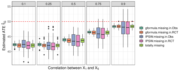
Figure 12: Simulations results when imputing (procedure 4): Results when imputing $X_{1}$ with a linear model fitted on the complete data set (either the RCT or the observational). All the missing covariate pattern are simulated using either the G-formula or the IPSW estimators. The impact of the correlation between $X_{1}$ and $X_{5}$ is investigated. Each simulation is repeated 100 times. All procedures have a similar bias as the procedure ignoring the partially-missing covariate (totally.missing), so that a linear imputation (procedure 4) improves neither the bias nor the variance.

Proxy variable

Finally and to illustrate Lemma 1, the simulation is extended to replace $X_{1}$ by a proxy variable, generated following (8) with a varying $\sigma_{prox}$. The generalized ATE is estimated with the G-formula. The experiments is repeated 20 times per $\sigma_{prox}$ values. Results are presented on Figure 13. Whenever $\sigma_{prox}$ is small compared to $\sigma_{mis}$ (which is equal to one in this simulation), therefore the bias is small.

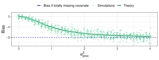
Figure 13: Simulation results for proxy variable (procedure 5) Simulation when a key covariate is replaced by a proxy following the proxy-framework (see Assumption 8). The theoretical bias (1) is represented along with the empirical values obtained when generalizing the ATE with the plugged-in G-formula estimator.

Appendix G Homogeneity of the variance-covariance matrix

Recall that Assumption 7 states that the covariance matrices in both data sets are identical. This assumption, which may appear to be very restrictive, can be partially tested on the set of observed covariates. In this section, we present such a test (Box’s M-test Box, 1949), which illustrates the validity of Assumption 7 on some particular data set. Taking one step further, we study the impact of Assumption 7 violation on the resutling estimate.

G.1 Statistical test and visualizations

Friendly and Sigal (2020) detail available tests to assess if covariance matrices from two data sample are equal. Despite its sensitivity to violation, Box’s M-test (Box, 1949) can be used test the equality. In particular the package heplots contains the tests and visualizations in R. The command line to perform the test is detailed below.

⬇

library(heplots)

boxM(data[, c("X1", "X2", "X3", "X4")], group = data$S)

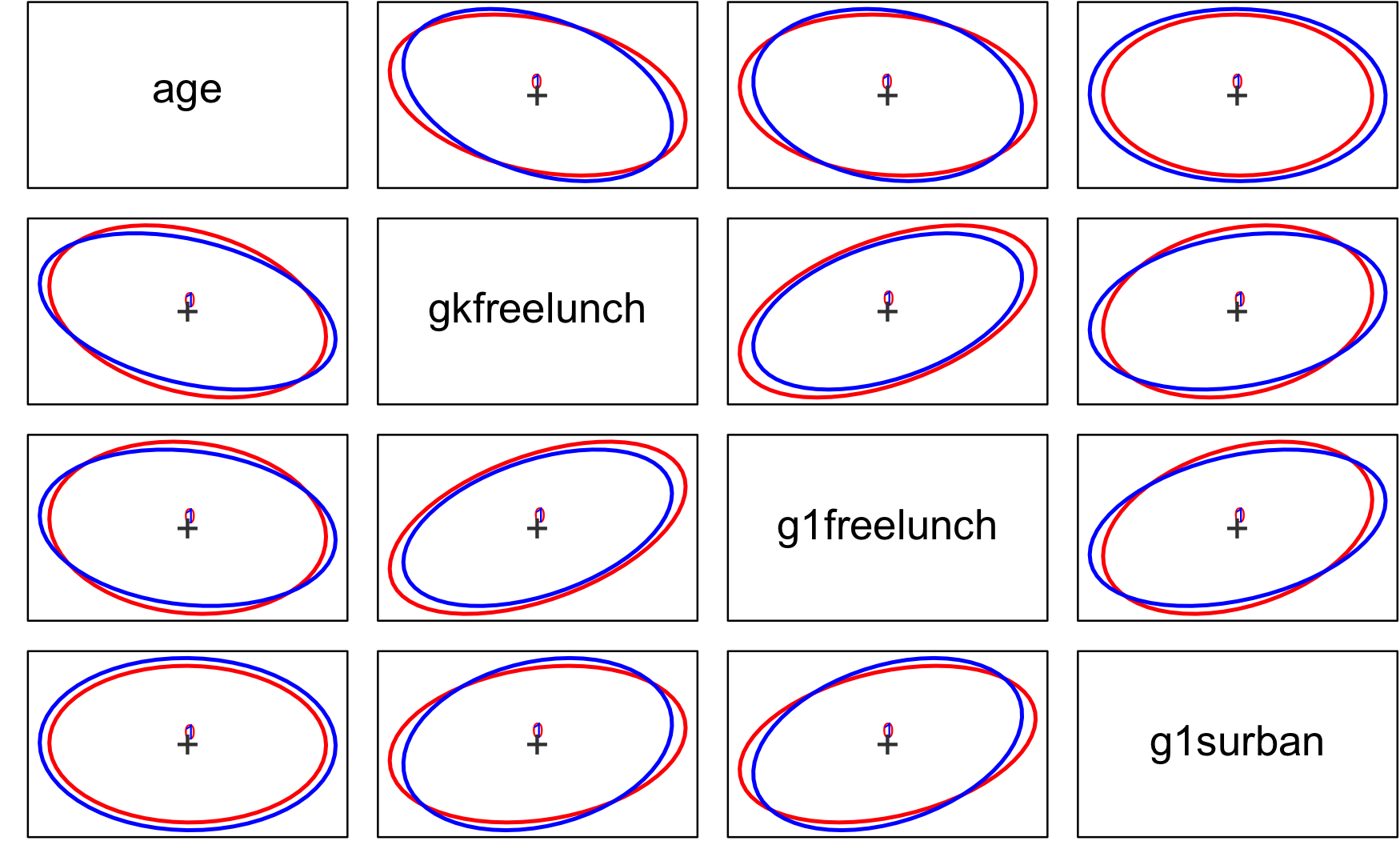
Figure 14: Pairwise data ellipses for the STAR data, centered at the origin. This view allows to compare the variances and covariances for all pairs of variables.

Even if we cannot bring a general rule to know if the covariance matrices are equal, we can display some examples in which Assumption 7 holds. For instance, Friendly and Sigal (2020) report that the skull data is an example of a real data set with multiple sources where there are substantial differences among the means of groups, but little evidence for heterogeneity of their covariance matrices.

G.1.1 Semi-synthetic experiment: STAR

While doing the semi-synthetic experiment on the STAR data set, the Box M-test rejects the null hypothesis when considering only numerical covariates (age, g1freelunch, gkfreelunch, and g1surban) with a p-value of 0.022. This indicates that the preservation of the variance-covariance structure between the two simulated sources does not hold. To help support conclusions, one can visualize how the variance covariance matrix vary in between the two sources, as presented on Figure 14, supporting that the changes in the variance-covariance are not very strong.

G.1.2 Traumabase and CRASH-3

Note that this part’s purpose is only to illustrate the principle as the application performed in Section 5 relies on the independence between the time to treatment and all other covariates, and not Assumption 7.

One can inspect how far the variance and covariance change in between the two sources. Pairwise data ellipses are presented on Figure 15 for CRASH-3 and Traumabase patients, suggesting rather strong difference in the variance-covariance matrix. As expected Box M-test largely rejects the null hypothesis.

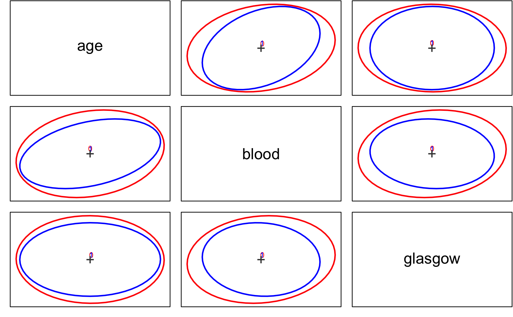
Figure 15: Pairwise data ellipses for the CRASH-3 and Traumabase data, centered at the origin. CRASH-3 data are in blue and Traumabase data in red. This view allows to compare the variances and covariances for all pairs of variables. While the mean are really different in the two sources, the variances and covariances are not so different.

It is interesting to note that in some cases the variance covariance matrix is identical in between two populations. For example we tested whether the two major trauma centers in France present heterogeneity in the variance-covariance matrix, and the Box M test does not reject the null hypothesis.

G.2 Extension of the simulations

Simulations presented in Section 4 can be extended to illustrate empirically the consequences of a poorly specified Assumption 7. Suppose $X_{1}$ is the unobserved covariate, and that the variance-covariance matrix is not the same in the randomized population ($S=1$) as in the target population. But the heterogeneities in between the two sources can be different in their nature, affecting covariates depending or not from $X_{1}$. We can imagine two situations, a situation (A) where the link in between $X_{1}$ and $X_{5}$ is different in the two sources, and another situation (B) where the link in between $X_{2}$ and $X_{3}$ is not the same. The situation is illustrated on Figures 16(a) and 16(b) with pairwise data ellipses. Note that with $n=1000$ and $m=10000$ a Box-M test largely rejects the null-hypothesis with a similar statistic value for both situations. When computing the bias according to Theorem 1 and repeating the experiment $50$ times, empirical evidence is made that the localization of the heterogeneity impacts or not the bias computation. As presented on Figure 16(c), situation A affects the bias computation, when situation B keeps the bias estimation valid.

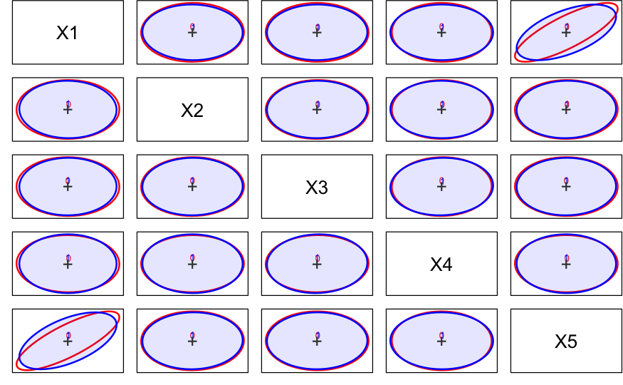
(a) Situation A - Centered pairwise data ellipses

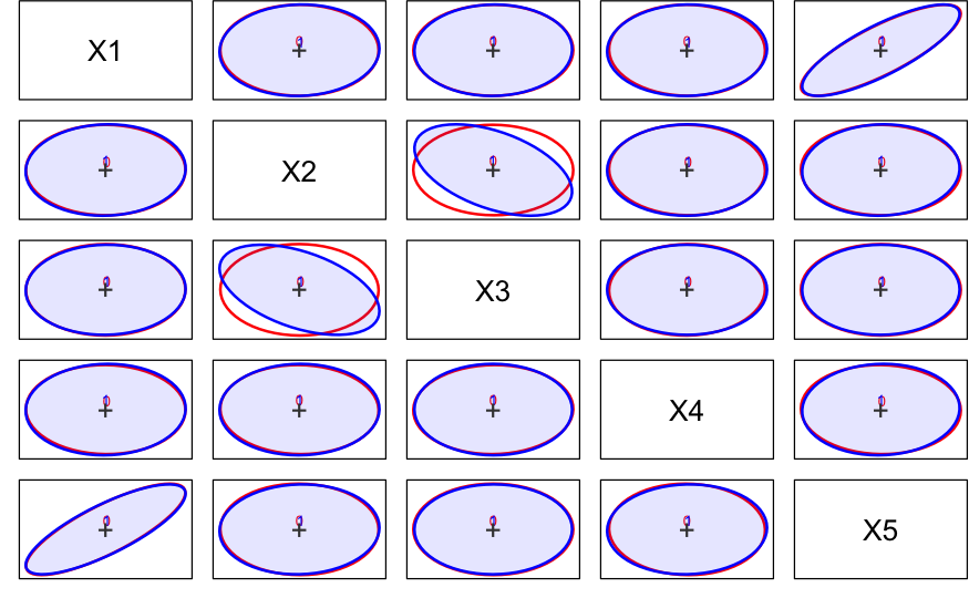
(b) Situation B - Centered pairwise data ellipses

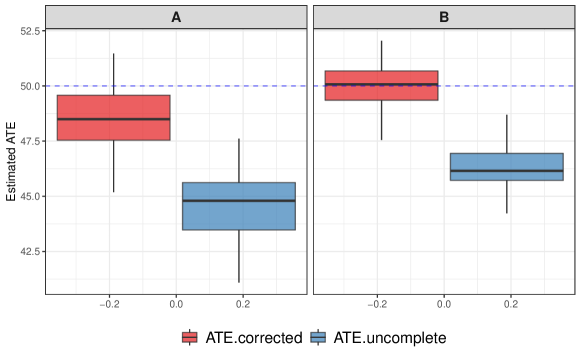
(c) ATE estimation in the two situations where $\hat{\tau}_{\text{\tiny G},obs}$ is estimated considering $X_{1}$ is missing and denoted ATE.uncomplete, while the bias $B$ is estimated following Theorem 1 giving ATE.corrected ($\hat{\tau}_{\text{\tiny G},obs}+\hat{B}$).

Figure 16: Effect of a different variance-covariance matrix on the ATE estimation, where heterogeneity between the two variance-covariance matrix is introduced as presented in (a) and (b), and on (c) the impact on the estimated average treatment effect (ATE). Situations A and B result in a similar statistics when using a Box-M test, but leads to very different impact on the bias estimation as visible on (c). The simulation are repeated 50 times, with a similar outcome generative model as in (8), and $n=1000$ and $m=10000$.

G.3 Recommendations

Our current recommendations when considering the Assumption 7 is, first, to visualize the heterogeneity of variance-covariance matrix with pairwise data ellipses on $\Sigma_{obs,obs}$. A statistical test such as a Box-M test can be applied on $\Sigma_{obs,obs}$. We also want to emphasize that a statistical test depends on the size of the data sample, when what really matters in this assumption for the sensitivity analysis to be valid is the permanence of covariance structure of the missing covariates with the strongly correlated observed covariates. Simulations presented on Figure 16(c) is somehow an empirical pathological case where the variance-covariance matrix are equivalently different when considering a statistical test, but leads to different consequences on the validity of Theorem 1, and therefore the sensitivity analysis.

G.4 Comment about the notations

The notations used in this work inherits from the generalization literature and reflects the idea of a plausibility to be sampled from a target superpopulation. The point of view of two population with support inclusion is equivalent for our purpose. Still, thinking to the problem of a sampling bias, then Assumption 7 imposes unusual restrictions for $P(X\mid S=0)$, that is a subpopulation of the target population. As we do not do any inference on that population and as it has no practical interpretation, we do not discuss this in this work.

References

- Andrews and Oster (2019) Andrews, I. and E. Oster (2019). A simple approximation for evaluating external validity bias. Economics Letters 178, 58–62.
- Angrist and Pischke (2008) Angrist, J. D. and J.-S. Pischke (2008, December). Mostly Harmless Econometrics: An Empiricist’s Companion. Princeton University Press.
- Bareinboim and Pearl (2013) Bareinboim, E. and J. Pearl (2013). A general algorithm for deciding transportability of experimental results. Journal of Causal Inference 1(1), 107–134.
- Bareinboim and Pearl (2016) Bareinboim, E. and J. Pearl (2016). Causal inference and the data-fusion problem. Proceedings of the National Academy of Sciences 113(27), 7345–7352.
- Bareinboim et al. (2014) Bareinboim, E., J. Tian, and J. Pearl (2014). Recovering from selection bias in causal and statistical inference. In Proceedings of the Twenty-Eighth AAAI Conference on Artificial Intelligence, AAAI’14, pp. 2410–2416. AAAI Press.
- Box (1949) Box, G. E. P. (1949, 12). A general distribution theory for a class of likelihood criteria. Biometrika 36(3-4), 317–346.
- Brenner et al. (2018) Brenner, A., M. Arribas, J. Cuzick, V. Jairath, S. Stanworth, K. Ker, H. Shakur-Still, and I. Roberts (2018). Outcome measures in clinical trials of treatments for acute severe haemorrhage. Trials 19, 533.
- Buchanan et al. (2018) Buchanan, A. L., M. G. Hudgens, S. R. Cole, K. R. Mollan, P. E. Sax, E. S. Daar, A. A. Adimora, J. J. Eron, and M. J. Mugavero (2018). Generalizing evidence from randomized trials using inverse probability of sampling weights. Journal of the Royal Statistical Society: Series A (Statistics in Society) 181, 1193–1209.
- Chattopadhyay et al. (2022) Chattopadhyay, A., E. R. Cohn, and J. R. Zubizarreta (2022). One-step weighting to generalize and transport treatment effect estimates to a target population.
- Chen et al. (2007) Chen, X., H. Hong, and D. Nekipelov (2007). Measurement error models.
- Chen et al. (2005) Chen, X., H. Hong, and E. Tamer (2005, 02). Measurement error models with auxiliary data. Review of Economic Studies 72, 343–366.
- Chernozhukov et al. (2017) Chernozhukov, V., D. Chetverikov, M. Demirer, E. Duflo, C. Hansen, W. Newey, and J. Robins (2017, 06). Double/debiased machine learning for treatment and structural parameters. The Econometrics Journal 21.
- Cinelli and Hazlett (2020) Cinelli, C. and C. Hazlett (2020, February). Making sense of sensitivity: extending omitted variable bias. Journal of the Royal Statistical Society Series B 82(1), 39–67.
- Cole and Stuart (2010) Cole, S. R. and E. A. Stuart (2010). Generalizing evidence from randomized clinical trials to target populations: The actg 320 trial. American Journal of Epidemiology 172, 107–115.
- Colnet et al. (2020) Colnet, B., I. Mayer, G. Chen, A. Dieng, R. Li, G. Varoquaux, J.-P. Vert, J. Josse, and S. Yang (2020). Causal inference methods for combining randomized trials and observational studies: a review.
- Cornfield et al. (1959) Cornfield, J., W. Haenszel, E. C. Hammond, A. M. Lilienfeld, M. B. Shimkin, and E. L. Wynder (1959, 01). Smoking and Lung Cancer: Recent Evidence and a Discussion of Some Questions. JNCI: Journal of the National Cancer Institute 22(1), 173–203.
- Correa et al. (2018) Correa, J., J. Tian, and E. Bareinboim (2018). Generalized adjustment under confounding and selection biases.
- CRASH-3 (2019) CRASH-3 (2019). Effects of tranexamic acid on death, disability, vascular occlusive events and other morbidities in patients with acute traumatic brain injury (CRASH-3): a randomised, placebo-controlled trial. The Lancet 394(10210), 1713–1723.
- Dahabreh et al. (2020) Dahabreh, I. J., S. E. Robertson, J. A. Steingrimsson, E. A. Stuart, and M. A. Hernán (2020). Extending inferences from a randomized trial to a new target population. Statistics in Medicine 39(14), 1999–2014.
- Dahabreh et al. (2019) Dahabreh, I. J., S. E. Robertson, E. J. T. Tchetgen, E. A. Stuart, and M. A. Hernán (2019). Generalizing causal inferences from individuals in randomized trials to all trial-eligible individuals. Biometrics 75, 685–694.
- Dahabreh et al. (2019) Dahabreh, I. J., J. M. Robins, S. J. Haneuse, and M. A. Hernán (2019). Generalizing causal inferences from randomized trials: counterfactual and graphical identification. arXiv preprint arXiv:1906.10792.
- Dahabreh et al. (2019) Dahabreh, I. J., J. M. Robins, S. J.-P. A. Haneuse, I. Saeed, S. E. Robertson, E. A. Stuart, and M. A. Hernán (2019). Sensitivity analysis using bias functions for studies extending inferences from a randomized trial to a target population.
- Degtiar and Rose (2021) Degtiar, I. and S. Rose (2021). A review of generalizability and transportability.
- Dewan et al. (2012) Dewan, Y., E. Komolafe, J. Mejìa-Mantilla, P. Perel, I. Roberts, and H. Shakur-Still (2012, 06). CRASH-3: Tranexamic acid for the treatment of significant traumatic brain injury: study protocol for an international randomized, double-blind, placebo-controlled trial. Trials 13, 87.
- Ding et al. (2016) Ding, P., A. Feller, and L. Miratrix (2016, June). Randomization inference for treatment effect variation. Journal of the Royal Statistical Society Series B 78(3), 655–671.
- Dong et al. (2020) Dong, L., S. Yang, X. Wang, D. Zeng, and J. Cai (2020). Integrative analysis of randomized clinical trials with real world evidence studies. arXiv preprint arXiv:2003.01242.
- Dorie et al. (2016) Dorie, V., M. Harada, N. Carnegie, and J. Hill (2016, September). A flexible, interpretable framework for assessing sensitivity to unmeasured confounding. Statistics in Medicine 35(20), 3453–3470.
- Egami and Hartman (2021) Egami, N. and E. Hartman (2021, 08). Covariate selection for generalizing experimental results: Application to a large‐scale development program in uganda*. Journal of the Royal Statistical Society: Series A (Statistics in Society) 184.
- Finn and Achilles (1990) Finn, J. D. and C. M. Achilles (1990). Answers and questions about class size: A statewide experiment. American Educational Research Journal 27(3), 557–577.
- Franks et al. (2019) Franks, A., A. D’Amour, and A. Feller (2019, 04). Flexible sensitivity analysis for observational studies without observable implications. Journal of the American Statistical Association, 1–38.