Nonlinear dynamics of flux compactification

Abstract

We study the nonlinear evolution of unstable flux compactifications, applying numerical relativity techniques to solve the Einstein equations in $D$ dimensions coupled to a $q$-form field and positive cosmological constant. We show that initially homogeneous flux compactifications are unstable to dynamically forming warped compactifications. In some cases, we find that the warping process can serve as a toy-model of slow-roll inflation, while in other instances, we find solutions that eventually evolve to a singular state. Analogous to dynamical black hole horizons, we use the geometric properties of marginally trapped surfaces to characterize the lower dimensional vacua in the inhomogeneous and dynamical settings we consider. We find that lower-dimensional vacua with a lower expansion rate are dynamically favoured, and in some cases find spacetimes that undergo a period of accelerated expansion followed by contraction.

1 Introduction

The standard cosmological model invokes accelerated expansion of the Universe both at early times, in an inflationary era, and at late times, in the current epoch of dark energy domination. Determining the physical mechanism(s) responsible for the accelerated expansion of the Universe is among the most important challenges in modern cosmology. One proposed framework for tackling this is string/M-theory, where the mechanisms responsible for dark energy and inflation would ideally just be one feature of a complete description of gravity and the standard model of particle physics.

A major complication in developing these phenomenological connections are the extra spatial dimensions invoked to make string theory a consistent quantum theory of gravity. There are two dominant paradigms for explaining why we cannot experimentally probe extra spatial dimensions: they are small (compactification Kaluza:1921tu ; Klein:1926tv ) or the standard model degrees of freedom are constrained to move in only four dimensions (the braneworld scenario ArkaniHamed:1998rs ; Randall:1999ee ; Randall:1999vf ). The specific choice of compactification or realization of the braneworld scenario has implications for phenomenology, dictating the particle content and vacuum structure, as well as the types and strengths of interactions, in the effectively four-dimensional theory that results. The proliferation of four-dimensional theories (known as the string theory landscape Susskind:2003kw ) intertwines string theory with cosmology in many fundamental ways. In this paper, our main point of contact will be the evolution of the size and shape of a compactification, which (in this picture) are part of our cosmological history, and can provide the physical mechanism for inflation and dark energy.

What dynamics might be associated with extra dimensions? In the simplest scenario, the Universe remains effectively four-dimensional and small deformations of the extra dimensions correspond to a set of fields known as Kaluza Klein (KK) modes. Even this is highly non-trivial, requiring the addition of various sources of energy momentum (such as $q$-form gauge fields, branes, etc.) to stabilize the size and shape of the compactification, and verifying that the resulting four-dimensional effective theory has the desired properties. Beyond studying linear perturbations of such static stable configurations, very little is known about the dynamics associated with extra dimensions. This is not surprising given the difficulties in solving Einstein’s equations in four dimensions, let alone ten. Nevertheless, a better understanding is necessary to fully understand cosmology in theories with extra dimensions, and in particular address questions such as: How was the Universe we observe selected from the many possibilities? What features of our Universe are accidental, and which are inevitable (e.g. fixed by special initial conditions or symmetries)? Why are there only three large spatial dimensions?

To make progress in this direction, we focus on a simple model that retains many of the important features of the low-energy limit of string theory: Einstein-Maxwell theory in $D$-dimensions with a positive cosmological constant and a $q$-form gauge field. Freund and Rubin Freund:1980 showed that this theory admits solutions in which the extra dimensions are compactified on a sphere, stabilized against collapse by the positive curvature of the compactification and a homogeneous configuration of the gauge field over the sphere. If a positive bulk cosmological constant is included Bousso:2003 , it is possible to find solutions in $D=p+q$ dimensions that are a product space of $p$-dimensional anti-de Sitter, Minkowski or de Sitter space and a $q$-dimensional sphere. The size of the compact sphere and the magnitude of the four dimensional cosmological constant are adjusted with the number of units of flux of the $q$-form gauge field wrapping the $q$-sphere. This simple model figures prominently in the AdS/CFT correspondence Maldacena:1997re , serves as a simple example of flux compactifications in string theory Douglas:2006es ; Denef:2007pq , and has been employed to study the cosmological constant problem Denef:2007pq ; Carroll:2009dn ; Brown:2013fba ; Asensio:2012pg , flux tunneling Aguirre:2009tp ; BlancoPillado:2009di ; Brown:2010bc ; BlancoPillado:2010et , and dimension-changing transitions Contaldi:2004hr ; Krishnan:2005 ; Carroll:2009dn ; BlancoPillado:2009mi , among other phenomena. Another interesting feature of the Einstein-Maxwell model is that in addition to spherical compactifications, it also admits stable solutions where the compact space is inhomogeneous, or “warped" Kinoshita:2007 ; Kinoshita:2009hh ; Lim:2012 ; Dahlen:2014 . In string constructions, warped extra dimensions are essential in models that address the hierarchy between the gravitational and electroweak scales Giddings:2001yu , dark energy Kachru:2003aw , and cosmic inflation (e.g. Kachru:2003sx ). A complete understanding of the dynamical generation of such structure is an important missing component of the cosmology of these models.

In the Einstein-Maxwell model, the linear stability and mass spectrum of the Freund-Rubin solutions were studied in refs. DeWolfe:2001nz ; Kinoshita:2007 ; Kinoshita:2009hh ; Lim:2012 ; Brown:2013 ; Hinterbichler:2014 . Their analysis showed that the stability of the solution to small perturbations depends on the relative value of the flux density or Hubble parameter compared to the cosmological constant as well as on the dimension of the internal manifold. There are two types of dynamical instabilities:

• The total volume instability can be attributed to homogeneous perturbations ($\ell=0$ modes) of the internal space and arises whenever the density of flux lines warping the $q$-sphere is too small, or equivalently, when the Hubble expansion rate of the external de Sitter space is too large causing the internal manifold to either grow or shrink. The endpoint of this instability was found to be either decompactification to empty $D$-dimensional de Sitter space or flow in towards a different configuration where total flux integrated over the compact space is the same but the volume is smaller hence flux density larger Krishnan:2005 .

• The warped instability arises when $q\geq 4$ (in contrast to the volume instability which already exists when $q\geq 2$) and is due to inhomogeneous perturbations. Mathematically, this instability is due to a mode that couples the metric and flux (with $\ell\geq 2$ angular dependence) and in turn deforms the internal space. One expects that if some configuration is unstable for a given total flux, then this may signal the presence of another more stable configuration with the same flux. Indeed refs. Kinoshita:2007 ; Lim:2012 ; Dahlen:2014 numerically constructed stationary warped solutions and ref. Kinoshita:2009hh studied their perturbative stability. But their connection to the inhomogeneous instability has not been determined, so it is not known whether these are the endpoint of the instability.

Note that when $q\geq 5$, all of the Freund-Rubin solutions are linearly unstable to one or both types of instability.

The goal of this paper is to go beyond studying stationary or homogeneous solutions, and their linear perturbations, by performing full nonlinear evolutions of perturbed Freund-Rubin and warped compactifications. We do this by applying modern numerical relativity techniques to probe the inhomogeneous and strong field regime, as has been done for a number of different cosmological scenarios, e.g. Garfinkle:2008ei ; Wainwright:2013lea ; East:2015ggf ; East:2016anr ; Clough:2016ymm , though here we study inhomogeneities in a compact extra dimension. We find rich dynamics, in some cases finding evolution from unstable to stable stationary warped solutions, though in other cases finding that unstable solutions evolve towards a singular state (even in some cases overshooting stable stationary solutions). We comment on some features of the cosmology seen by four-dimensional observers, and motivate the use of the cosmological apparent horizon as a useful measure of the four dimensional Hubble parameter. The solutions we study provide an important proof-of-principle that numerical relativity could be a powerful tool for exploring new phenomena in cosmologies with extra spatial dimensions.

2 Flux compactifications in Einstein-Maxwell theory

In this paper, we focus on solutions to Einstein-Maxwell theory in $D=p+q$ spacetime dimensions with a $D$-dimensional cosmological constant $\Lambda_{D}$ and a $q$-form flux that wraps $q$ compact dimensions, leaving $p$ uncompactified dimensions. The starting point for the theory is then the following $D=p+q$-dimensional action

$$S=\int d^{p}xd^{q}y\sqrt{-g}\bigg{[}\frac{1}{2}{}^{(D)}R-\Lambda_{D}-\frac{1}{2q!}\mathbf{F}_{q}^{2}\bigg{]}$$ (1)

where we use units with $M_{D}=c=1$, where $M_{D}\equiv\left(8\pi G_{D}\right)^{-1/(D-2)}$ is the $D$-dimensional Planck mass, ${}^{(D)}R$ is the $D$-dimensional scalar curvature, and $\mathbf{F}_{q}=F_{M_{1}...M_{q}}$ is a $q$-form. Note this choice of units is not conventional, but it leaves us the freedom to fix $\Lambda_{D}$.

The Einstein equations which follow from the action (1) are

$$G_{MN}={}^{(D)}R_{MN}-\frac{1}{2}{}^{(D)}Rg_{MN}=T_{MN}$$ (2)

where the stress-energy tensor is

$$T_{MN}=\frac{1}{(q-1)!}F_{MP_{2}...P_{q}}F_{N}^{P_{2}...P_{q}}-\frac{1}{2q!}\mathbf{F}_{q}^{2}g_{MN}-\Lambda_{D}g_{MN}$$ (3)

with $\mathbf{F}_{q}^{2}=F_{M_{1}...M_{q}}F^{M_{1}...M_{q}}$. The equations governing the $q$-form in the absence of sources are

$$\nabla_{[N}F_{MP_{2}...P_{q}]}=\nabla^{M}F_{MP_{2}...P_{q}}=0\ .$$ (4)

Throughout the paper we will use $M$, $N$, …to denote indices that run over the $D-$dimensions, $\overline{m}$, $\overline{n}$, …for $(D-1)$-dimensional spatial indices, $\mu$, $\nu$, …for $p=4$-dimensional spacetime indices, and $\alpha,\beta,\ldots$ for $q$-dimensional spatial indices.

The simplest flux compactifications of Einstein Maxwell theory are the Freund-Rubin solutions Freund:1980 : product spaces $\mathcal{M}_{p}\times S_{q}$, where $\mathcal{M}_{p}$ is a maximally symmetric p-dimensional spacetime and $S_{q}$ is a q-dimensional sphere. In this paper, we investigate solutions that are warped along a single internal direction, the polar angle $\theta$. That is, we study solutions such that the $p$-dimensional external space is homogeneous in the uncompactified spatial dimensions with a warp factor depending on $\theta$, and the $q$-dimensional compact space has the topology of a sphere with $q-1$ azimuthal symmetries. With these symmetries, the metric takes the form:

$$\begin{array}[]{lcl}ds^{2}&=&-(\alpha^{2}-\beta_{\theta}\beta^{\theta})dt^{2}+\gamma_{xx}(\theta,t)d{\vec{x}^{2}}_{p-1}+2\gamma_{\theta\theta}(\theta,t)\beta^{\theta}dtd\theta\\ &&+\gamma_{\theta\theta}(\theta,t)d\theta^{2}+\gamma_{\phi_{1}\phi_{1}}(\theta,t)d\Omega^{2}_{q-1}\end{array}$$ (5)

where $d\Omega^{2}_{q-1}=d\phi_{1}^{2}+\sin^{2}\phi_{1}d\Omega^{2}_{q-1}$, $\alpha(\theta,t)$ is the lapse and $\beta^{\theta}(\theta,t)$ is by symmetry the only non-zero component of the shift vector.

The $q$-form flux is time-dependent and non-uniformly distributed in the $\theta$-direction,

$$\begin{array}[]{lcl}\mathbf{F}_{q}&=&Q_{B}(\theta,t)N(\theta,\phi_{1},\dots,\phi_{q-1})d\theta\wedge\dots\wedge d\phi_{q-1}\vspace{1em}\\ &&-\alpha Q_{E}(\theta,t)N(\theta,\phi_{1},\dots,\phi_{q-1})dt\wedge d\phi_{1}\wedge\dots\wedge d\phi_{q-1}\end{array}$$ (6)

where $N(\theta,\phi_{1},...,\phi_{q-1})=\sin^{q-1}\theta\sin^{q-2}\phi_{1}...\sin\phi_{q-2}$ and $Q_{B}(\theta,t)$ and $Q_{E}(\theta,t)$ represent the magnetic and electric flux strengths, respectively.

In the remainder of this section, we review a variety of features of flux compactifications in Einstein-Maxwell theory. In section 2.1, we define several quantities that will be useful in describing solutions. In section 2.2, we outline how to describe the cosmology of the non-compact space. In section 2.3, we review the Freund-Rubin solutions and their stability. Finally, in section 2.4, we review the warped compactifications of refs. Kinoshita:2007 ; Kinoshita:2009hh . The reader interested in going directly to the results can proceed to section 4.

2.1 Characterizing the solutions

We now define a few quantities which are helpful in describing the solutions presented below. The compact space is characterized by the volume of the internal $q$-sphere

$$\textbf{Vol}_{S^{q}}\equiv\int\sqrt{\gamma_{q}}d^{q}y=\int\sqrt{\gamma_{q}}d\theta\wedge d\phi_{1}\wedge...\wedge d\phi_{q-1}\ ,$$ (7)

the total number of flux units, which is a conserved quantity obtained by integrating the flux density over the internal $q$-sphere,

$$n\equiv\int_{S_{q}}\mathbf{F}_{q}\ ,$$ (8)

and the aspect ratio

$$\epsilon=\frac{\int_{0}^{\pi}\sqrt{\gamma_{\theta\theta}(\theta,t)}d\theta}{\pi\sqrt{{\widetilde{\gamma}}_{\phi_{1}\phi_{1}}(\pi/2,t)}}\ ,$$ (9)

defined such that spherical solutions have $\epsilon=1$, oblate solutions have $\epsilon<1$ and prolate solutions have $\epsilon>1$.

As a visualisation tool, we also plot the internal metric as an embedding in $q+1$ Euclidean dimensions. The internal metric $ds^{2}=\gamma_{\theta\theta}d\theta^{2}+\widetilde{\gamma}_{\phi_{1}\phi_{1}}\sin^{2}\theta d{\Omega_{q-1}}^{2}$ is the induced metric on the surface

$$\begin{array}[]{lcl}x_{1}&=&\int^{\theta}_{\pi/2}d\theta^{\prime}\sqrt{\gamma_{\theta^{\prime}\theta^{\prime}}(\theta^{\prime},t)-\left[\partial_{\theta^{\prime}}\left(\widetilde{\gamma}_{\phi_{1}\phi_{1}}(\theta^{\prime},t)^{1/2}\sin\theta^{\prime}\right)\right]^{2}}\vspace{1em}\\ x_{2}&=&\widetilde{\gamma}_{\phi_{1}\phi_{1}}(\theta,t)^{1/2}\sin\theta\cos\phi_{1}\vspace{1em}\\ x_{3}&=&\widetilde{\gamma}_{\phi_{1}\phi_{1}}(\theta,t)^{1/2}\sin\theta\sin\phi_{1}\cos\phi_{2}\vspace{1em}\\ \vdots\vspace{1em}\\ x_{q}&=&\widetilde{\gamma}_{\phi_{1}\phi_{1}}(\theta,t)^{1/2}\sin\theta\ldots\sin\phi_{q-2}\cos\phi_{q-1}\vspace{1em}\\ x_{q+1}&=&\widetilde{\gamma}_{\phi_{1}\phi_{1}}(\theta,t)^{1/2}\sin\theta\ldots\sin\phi_{q-2}\sin\phi_{q-1}\ .\end{array}$$

2.2 The lower dimensional cosmology

If one hopes to make contact with the observable Universe, it is necessary to determine the effective four-dimensional cosmology sourced by evolution of the compact extra dimensions. The standard approach is via the procedure of “dimensional reduction", where one integrates the action over the compact extra dimensions and identifies a four-dimensional gravitational sector and a set of moduli fields associated with properties of the compactification, such as the total volume (see e.g. refs. DeWolfe:2002nn ; Giddings:2001yu for an approach most relevant to the present context). This approach has several limitations. Perhaps most importantly, because one must identify a set of coordinates to integrate over, dimensional reduction is intrinsically gauge dependent. Furthermore, gauge dependence arises when identifying the four-dimensional gravitational sector and moduli fields; it is typically feasible to do so only in special coordinate systems where the symmetries of the spacetime are manifest. Without prior knowledge of the “right" coordinate system, it is typically only possible to study small perturbations (see e.g. refs. Giddings:2005ff ; Frey:2008xw ). In the context of numerical relativity, one does not have complete freedom to dictate the coordinate system most convenient for dimensional reduction: in general, it is necessary to specify the gauge dynamics in a way that leads to well-posed evolution, while avoiding coordinate singularities. Another challenge is that in the typical approach to dimensional reduction, the goal is to find a set of equations of motion for the four-dimensional variables, while our starting point is the solution itself. Given a solution and not the four-dimensional equations of motion, it may not be possible to unambiguously identify the appropriate four-dimensional variables. These subtleties motivate an alternative approach based on the geometrical properties of the solutions themselves, which we now outline. Note, to make contact with the observable universe we assume $p=4$.

To motivate our approach, let us recall some properties of the standard FLRW solution in four dimensions:

$$ds^{2}=-\alpha^{2}(t)dt^{2}+a^{2}(t)(dx^{2}+dy^{2}+dz^{2})\ .$$ (10)

The extrinsic curvature of spatial slices is $K_{ii}=-a(da/d\tau)$, with $d/d\tau\equiv(1/\alpha)d/dt$, for $i=x$, $y$ and $z$, and the trace is

$$K=3{K^{x}}_{x}=-\frac{d\ln{\rm Vol}_{3}}{d\tau}=-\frac{3}{a}\frac{da}{d\tau}\equiv-3H.$$ (11)

where $H$ is the Hubble parameter and ${\rm Vol}_{3}=\sqrt{\gamma}=a^{3}$ is the normalized volume enclosed by a congruence of comoving geodesics. Note that these equalities are contingent on the time slicing chosen here, which preserves the homogeneity of the FLRW solution. In this cosmological slicing, the trace of the extrinsic curvature (or equivalently the expansion of comoving timelike geodesics) determines the Hubble parameter. Another useful geometrical quantity is the area of the cosmological apparent horizon. We define the cosmological apparent horizon as a surface where the null expansion vanishes. (This is analogous to how apparent horizons can be used to define black hole horizons on a specific timeslice.) In an expanding FLRW universe, the coordinate radius of the cosmological apparent horizon is simply the comoving Hubble radius $r_{H}=(aH)^{-1}$, yielding an area:

$$\mathcal{A}_{H}=4\pi a^{2}r_{H}^{2}=4\pi H^{-2}$$ (12)

Therefore, we see that both the extrinsic curvature and the area of the cosmological apparent horizon can be used as alternative definitions of the Hubble parameter:

$$H=-\frac{K}{3}=\sqrt{\frac{4\pi}{\mathcal{A}_{H}}}\ ,$$ (13)

where again the equivalence with the usual definition of the Hubble parameter is contingent on choosing a cosmological slicing.

How does this picture generalize to the present context, where we have compact extra dimensions? The trace of the intrinsic curvature in this case depends on the position in the compact space and contains terms associated with the expansion of the volume in the compact space:

$$K(\theta,t)=3{K^{x}}_{x}+{K^{\theta}}_{\theta}+(q-1){K^{\phi_{1}}}_{\phi_{1}}=-\left(\frac{d\ln{\rm Vol}_{3}}{d\tau}+\frac{d\ln{\rm Vol}_{q}}{d\tau}\right)$$ (14)

where for a general slicing, $d/d\tau\equiv(1/\alpha)(\partial_{t}-\mathcal{L}_{\beta})$, where the last term is the Lie derivative with respect to the shift vector. The observers associated with a general time slicing will not necessarily follow geodesics in the full D-dimensional spacetime, and restricting to geodesic slicing can be problematic due to the appearance of coordinate singularities. This aside, there are other subtleties associated with finding an effective four-dimensional Hubble parameter from the extrinsic curvature. If we were to use the trace of the extrinsic curvature, note that this includes expansion of both the compact and non-compact space. Should one simply use $-{K^{x}}_{x}$, which characterizes the expansion in the non-compact dimensions, or some combination of the expansion in the compact and non-compact space? In addition, the expansion is not homogeneous in the extra dimensions, so one must define the correct measure of integration over the compact space to obtain the expansion seen by an “average" cosmological observer.

Some insight to these questions can be gained by investigating the properties of the cosmological apparent horizon, which as we outlined above, can be used to define the Hubble parameter in a four-dimensional FLRW Universe. For surfaces of constant time and (uncompactified) radius $r\equiv\sqrt{x^{2}+y^{2}+z^{2}}$ with unit inward (outward) normal $s^{\bar{m}}$ the inward (outward) null expansion

$$\Theta_{\mp}=D_{\bar{m}}s^{\bar{m}}+K_{\bar{m}\bar{n}}s^{\bar{m}}s^{\bar{n}}-K$$ (15)

vanishes on the surface

$$r_{H} = \frac{\pm 2}{\sqrt{\gamma_{xx}}}\frac{1}{({K^{x}}_{x}-K)}\ .$$ (16)

A marginally inner trapped surface with $\Theta_{-}=0$ and $\Theta_{+}>0$ is a generalization of the de Sitter horizon, while the marginally outer trapped surface with $\Theta_{+}=0$ and $\Theta_{-}<0$ that occurs for contracting spacetimes is more similar to that of a black hole apparent horizon.

The area of the cosmological apparent horizon is obtained by integrating over the compact space

$$\mathcal{A}_{H}(t) = \int d\theta d\phi_{1}\cdots d\phi_{q-1}\sqrt{\gamma_{q}}\ 4\pi r_{H}^{2}\gamma_{xx}$$ (17)

$$= \int d\theta d\phi_{1}\cdots d\phi_{q-1}\sqrt{\gamma_{q}}\ 4\pi\left(\frac{2}{{K^{x}}_{x}-K}\right)^{2}\ .$$ (18)

Note that this is a $q+2$ dimensional area with units of $L^{q+2}$ where $L$ is some length scale. One can also use this area as a measure of entropy:

$$\mathcal{S}\equiv 2\pi\mathcal{A}_{H}\ ,$$ (19)

where we recall that in our units $M_{D}\equiv(8\pi G_{D})^{-1/(D-2)}=1$. The connection between the area of the apparent horizon and gravitational entropy is related to the thermodynamic interpretation of Einstein’s equations Jacobson:1995ab ; Padmanabhan:2002sha and has been considered for black holes (e.g. ref. Hayward:1998ee ) and cosmological spacetimes (e.g. refs. Frolov:2002va ; Cai:2005ra ; GalvezGhersi:2011tx ). In ref. Kinoshita:2009hh , it was shown that for a subset of the solutions we consider below, the entropy as defined above is a useful indicator of stability. In particular, for solutions at fixed conserved flux, the stable solution has the highest entropy. Note that since this analysis is entirely classical, one could simply use the area of the cosmological horizon as a measure of stability. As for a purely four-dimensional FLRW Universe, a Hubble parameter can be defined by

$$\frac{H}{M_{4}}\equiv\pm\sqrt{\frac{4\pi}{\mathcal{A}_{H}}}$$ (20)

where we take the positive (negative) sign when the inward (outward) null expansion vanishes. In our results below where we wish to examine the effective four-dimensional cosmology, we will use this definition of the Hubble parameter. Finally, we define the four-dimensional Planck mass as

$$M_{4}^{2}\equiv\int d\theta d\phi_{1}\cdots d\phi_{q-1}\sqrt{\gamma_{q}(t=0,\theta)}\ ,$$ (21)

where $\gamma_{q}$ refers to the background solution.

It is useful to examine the Hamiltonian constraint equation in order to make a more direct connection with the effective four-dimensional theory. This is given by

$$K^{2}-K_{\bar{m}\bar{n}}K^{\bar{m}\bar{n}}=2\rho-{}^{(D-1)}R$$ (22)

where $\rho=n^{N}n^{M}T_{MN}$ and ${}^{(D-1)}R$ is the intrinsic curvature on spatial slices. The extrinsic curvature term decomposes as follows

$$K_{\bar{m}\bar{n}}K^{\bar{m}\bar{n}}-K^{2} = -6\left(\frac{{K^{x}}_{x}-K}{2}\right)^{2}+\frac{1}{2}({K^{\theta}}_{\theta})^{2}+\frac{(q+3)(q-1)}{4}({K^{\phi}}_{\phi})^{2}$$

$$+ \left({K^{\theta}}_{\theta}+\frac{q-1}{2}{K^{\phi}}_{\phi}\right)^{2}\ .$$

Note that choosing to isolate the factor of $({K^{x}}_{x}-K)/2$, which appeared in the expression for the cosmological apparent horizon, nicely splits the extrinsic curvature term into negative definite and positive definite components. Re-arranging the Hamiltonian constraint equation we obtain:

$$\left(\frac{{K^{x}}_{x}-K}{2}\right)^{2}=\frac{1}{3M_{4}^{2}}\rho_{\rm eff}(\theta,t)$$ (24)

where we have defined

$$\rho_{\rm eff}(\theta,t)/M_{4}^{2} \equiv \rho-\frac{1}{2}{}^{(D-1)}R+\frac{1}{4}({K^{\theta}}_{\theta})^{2}+\frac{(q+3)(q-1)}{8}({K^{\phi}}_{\phi})^{2}$$

$$+ \frac{1}{2}\left({K^{\theta}}_{\theta}+\frac{q-1}{2}{K^{\phi}}_{\phi}\right)^{2}\ .$$

Equation (24) has the form of the Friedmann equation. The expression for the apparent horizon area eq. (17) can be used to define the measure of integration over the Hamiltonian constraint equation to give a four-dimensional Friedmann equation. In particular,

$$H(t)^{2}=\frac{1}{3M_{4}^{2}}\langle\rho_{\rm eff}(t)\rangle=\frac{4\pi M_{4}^{2}}{\mathcal{A}_{H}(t)}\ ,$$ (26)

where $H$ is defined as in eq. (20) and

$$\langle\rho_{\rm eff}(t)\rangle\equiv M_{4}^{2}\left[\int d\theta d\phi_{1}\cdots d\phi_{q-1}\sqrt{\gamma_{q}}\ (\rho_{\rm eff}(\theta,t))^{-1}\right]^{-1}\ .$$ (27)

Note that with these definitions, the square of the Hubble parameter is inversely proportional to the entropy, so a stability criterion based on maximizing the entropy (or synonymously, the area) is equivalent to one that minimizes this definition for the Hubble parameter.

For completeness, and because it will be useful in characterizing the properties of the solutions presented below, we sketch the standard procedure of dimensional reduction; further details can be found in appendix A. We begin with the D-dimensional action in ADM form:

$$S = \frac{1}{2}\int d^{4}xd^{q}y\sqrt{-g}\left[K_{\bar{m}\bar{n}}K^{\bar{m}\bar{n}}-K^{2}+{}^{(D-1)}R-2\Lambda_{D}-\frac{1}{q!}\mathbf{F}_{q}^{2}\right]\ .$$ (28)

The goal is to find an effective action for the four-dimensional metric variables and moduli fields, which can be identified with integrals of combinations of metric functions over the compact space (e.g. the volume). Schematically, for spacetimes that are homogeneous in the three large dimensions, the various terms in the action contribute as follows:

• $K_{\bar{m}\bar{n}}K^{\bar{m}\bar{n}}-K^{2}$: The extrinsic curvature term contains time derivatives of the metric functions, and therefore contains the 4-D Ricci scalar and kinetic terms for moduli fields.

• ${}^{(D-1)}R$: The Ricci scalar on spatial slices contains spatial derivatives of the metric functions on the compact space. With our assumption that the metric is independent of the three large dimensions, there are no contributions to the 4-D Ricci scalar. This term therefore contributes only to the potential for moduli fields.

• $2\Lambda_{D}+\mathbf{F}_{q}^{2}/q!$: The cosmological constant and flux terms contribute to the potential for moduli fields.

Here, we focus on the extrinsic curvature term; additional details for specific examples can be found in appendix A. Factoring the extrinsic curvature term as in Eq. (2.2), we have

$$S=\frac{1}{2}\int d^{4}xd^{q}y\sqrt{\gamma_{q}}\alpha\gamma_{xx}^{3/2}\left[-6\left(\frac{{K^{x}}_{x}-K}{2}\right)^{2}+\ldots\right]$$ (29)

Comparing this to the action for four dimensional FLRW solutions, one can try to equate:

$$\sqrt{-g(t)}\ M_{4}^{2}H(t)^{2}=\int d^{q}y\sqrt{\gamma_{q}}\alpha\gamma_{xx}^{3/2}\left(\frac{{K^{x}}_{x}-K}{2}\right)^{2}$$ (30)

For a convenient metric ansatz, one can explicitly identify $\sqrt{-g(t)}$, $M_{4}^{2}$ and $H(t)^{2}$; we outline several examples in appendix A. A nice feature of the decomposition of the extrinsic curvature we have chosen is that it contains the combination of metric functions that yield a dimensionally reduced action in the four dimensional Einstein frame (e.g. the conformal frame where $M_{4}$ is constant). For solutions with warping there are some subtleties in finding a unique four-dimensional metric determinant and Hubble parameter which we discuss in appendix A. In the more general cases we consider below, where we do not have complete freedom to specify a gauge where the metric functions take a convenient form, it is not possible to unambiguously identify the four dimensional Hubble parameter. We therefore utilize the geometrical definition of the Hubble parameter based on the area of the apparent horizon in Eq. 20.

2.3 Freund-Rubin branch

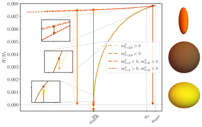
Figure 1: A cartoon of the Freund-Rubin and ellipsoidal solutions in the $(H/M_{4},n)$ plane for $\Lambda_{D}=1$ and $q=4$. For each value of the conserved flux number (8), there are two solutions: a symmetric solution where the compact space is spherical with an aspect ratio $\epsilon=1$ (indicated in brown), and a warped solution where the internal manifold is oblate with $\epsilon<1$ (yellow) or prolate with $\epsilon>1$ (orange). We find three critical values of $n$. First, for $n_{\mathrm{Mink}}<n<n_{\mathrm{max}}$ there are two Freund-Rubin and two warped solutions: On the Freund-Rubin branch there is a small and a large volume branch perturbatively stable or unstable to the volume instability ($m^{2}_{l=0}>0$ or $m^{2}_{l=0}<0$) respectively. At $n=n_{\mathrm{max}}$ the two branches merge and annihilate. On the warped branch there is one solution on the large Hubble warped branch, perturbatively unstable to the warped instability ($m^{2}_{l=2}<0$) and a solution on the small Hubble warped branch. At $n=n_{c}$ the small Hubble warped branch intersects the small volume Freund-Rubin branch and the two branches are marginally stable to the warped instability ($m^{2}_{l=2}=0$). Whenever the ellipsoidal solution has $\epsilon>1$ it is also perturbatively unstable. Arrows indicate the specific nonlinear solutions we discuss in section 4. They all point towards a solution with smaller effective Hubble rate and higher entropy (area). For a small range $n_{\mathrm{Mink}}\leq n<n_{I}$, solutions tend to a state where $H/M_{4}<0$, the cosmological implications of which are discussed in section 4.2.2

In this paper, we consider the nonlinear evolution of perturbations to two classes of stationary solutions of the theory described above. Namely, we consider the homogeneous Freund-Rubin solutions and warped solutions with a $\theta$-dependence. In the symmetric Freund-Rubin solution, a $q$-form flux uniformly wraps the extra dimensions into a $q$-sphere,

$$\mathbf{F}_{q}=\rho_{B}\textbf{vol}_{S^{q}}$$ (31)

where $\rho_{B}$ is the magnetic flux density and $\textbf{vol}_{S^{q}}=\epsilon$ is the volume element on the internal $q$-sphere. The direct product condition guarantees that the $p$ extended dimensions form an Einstein space. Restricting to the trivial case of a maximally symmetric extended de Sitter spacetime,

$$ds^{2}=-dt^{2}+e^{2Ht}d{\vec{x}^{2}}_{p-1}+L^{2}d\Omega_{q}^{2}$$ (32)

where $L$ is the radius of $q$-sphere, $H$ is the Hubble parameter (20) and in the particular case where $p=4$, $d{\vec{x}^{2}}_{p-1}=dx^{2}+dy^{2}+dz^{2}$ is the usual 3-Cartesian element.

The Maxwell equations are trivially satisfied, while the Einstein equations (2) enforce algebraic relations between the parameters $\{\rho_{b},H,L\}$

$${\Lambda_{D}}=\frac{(p-1)^{2}}{2}H^{2}+\frac{(q-1)^{2}}{2}L^{-2}$$ (33)

$$\rho_{B}^{2}=-(p-1)H^{2}+(q-1)L^{-2}$$ (34)

such that if we fix units with $\Lambda_{D}=1$, we are left with one free parameter describing the Freund-Rubin solutions. This parameter can be taken to be the total number of flux units (8)

$$n\equiv\int_{S_{q}}\mathbf{F}_{q}={\rho_{b}}\mathbf{Vol}_{S_{q}}\ ,$$ (35)

where the latter equality is specific to the Freund-Rubin solution. From (33) and (34), we can see that there can be more than one solution for a given value of $n$. Figure 1 shows these different solutions in $(H/M_{4},n)$ space. Focusing on the spherical solutions with aspect ratio $\epsilon=1$, the figure indicates that below some value $n_{\text{max}}$, there exists two solutions, a small and a large volume branch. As we will see below, the former is stable to the total-volume instability ($\ell=0$), but may be unstable to the warped instability ($\ell\geq 2$), while the latter is unstable to the total-volume instability, with the end point being decompactification or flow towards the small volume solution. For $n\geq n_{\text{max}}$, there is no solution.

2.3.1 The effective potential

In order to give some intuition for the stability of the flux compactification solutions, we can go back to the dimensional reduction procedure of section 2.2, and considering the source terms in eq. (28), think of the radius $L$ of the sphere as a four-dimensional radion field, living in an effective potential given by

$$\frac{V(L)}{M^{4}_{4}}=\frac{1}{2}\left(\frac{L_{0}}{L}\right)^{q}\left(-\frac{q(q-1)}{L^{2}}+2\Lambda_{D}+\frac{1}{M_{4}^{4}}\frac{n^{2}}{L^{2q}}\right)$$ (36)

The details of the derivation can be found in appendix A.1. From left to right, the three terms represent the spatial curvature, the higher dimensional vacuum energy, and the energy density of the flux, respectively. The flux term is repulsive, and tends to push the sphere to larger radius, but the curvature of the compact space is attractive, such that the interaction of these two terms can form a minimum of the potential where the radius of the $q$-sphere can be stabilized, yielding a four-dimensional vacuum.

Each allowed value of $n$, $p$ and $q$ defines a set of allowed radion potentials or landscape of lower dimensional theories. The potential for fixed $q=p=4$ and $\Lambda_{D}>0$ is sketched in figure 2 for a number of values of $n$. As we saw in the previous subsection, the number of extrema depends on the value of $n$. For small enough $n$, the effective potential has a minimum and a maximum corresponding to the small and large volume branches, respectively. The extrema merge at $n=n_{\text{max}}=81\pi^{2}/\left(\sqrt{2}\Lambda_{8}^{3/2}\right)$ and above this value there is no solution. Note that for small enough $n$ the four-dimensional vacua are negative, but as $n$ increases, they eventually become positive, which is important for cosmological solutions. To derive this effective potential, we assumed the shape of the compact space is fixed. However, we will see below that minima of the effective potential in figure 2 can be unstable maxima in other directions of the field-space that correspond to shape mode fluctuations.

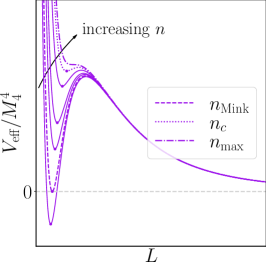
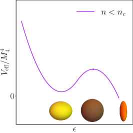
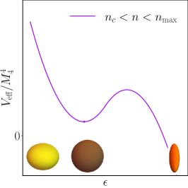
Figure 2: Left: The effective radion potential eq. (36) for $\Lambda_{D}>0$ and successively larger values of $n$ from bottom to top, assuming the compact space is spherically symmetric. The extrema correspond to the Freund-Rubin solutions. For small $n$, the effective potential has a maximum ($m^{2}_{\ell=0}<0$ and always de Sitter) and minimum ($m^{2}_{\ell=0}>0$ and de Sitter or anti-de Sitter). At $n=n_{\mathrm{max}}$ the solutions disappear. Right: Schematic of the effective potential for a fixed radius (minimum of $V_{\mathrm{eff}}(L)$), but changing ellipticity. We find that the effective potential tends to $+\infty/-\infty$ as the internal manifold becomes increasingly oblate or prolate, respectively. The Freund-Rubin solution is at a maximum ($m^{2}_{\ell=2}<0$) when the corresponding warped solution is oblate, and a minimum ($m^{2}_{\ell=2}>0$) when the warped solution is prolate. Some solutions escape the potential well of oblate solution to roll in the prolate direction.

2.3.2 Stability

We now briefly review linear perturbations around Freund-Rubin solutions, restricting to scalar-type perturbations with respect to, not only the $p$-dimensional external de Sitter space, but also the $SO(q)$ symmetry of the background internal space. The full perturbative spectrum was studied in refs. Brown:2013 ; Hinterbichler:2014 , and we defer the reader to those references for a more complete analysis. We write the perturbed metric as

$$\delta g_{\mu\nu}=-\frac{1}{p-2}g_{\mu\nu}\bar{h}Y_{\ell}(\theta)\ ,\qquad\delta g_{\alpha\beta}=\frac{1}{q}g_{\alpha\beta}\bar{h}Y_{\ell}(\theta)$$ (37)

which tells us that the $q$-sphere is deformed with the shape of a $m=0$ spherical harmonic $Y_{\ell}(\theta)$ and some amplitude $\bar{h}$.

The perturbed field strength is

$$\delta F_{\alpha_{1}...\alpha_{q}}=-\bar{a}\rho_{B}{\epsilon}_{\alpha_{1}...\alpha_{q}}\lambda_{\ell}Y_{\ell}(\theta)\ ,\qquad\delta F_{\beta\beta_{2}...\beta_{q}}=\nabla_{\beta}\bar{a}\rho_{B}{\epsilon}^{\alpha}_{\beta_{2}...\beta_{q}}\nabla_{\alpha}Y_{\ell}(\theta)$$ (38)

where $\lambda_{\ell}=\ell(\ell+q-1)/L^{2}>0$ is the eigenvalue of the spherical harmonic, $\Box_{y}Y_{\ell}(\theta)=-\lambda_{\ell}Y_{\ell}(\theta)$ (recalling that $y$ refers to the $q$-dimensional coordinates) and $\bar{a}$ is a dimensionless function. Note that the equations require that $\bar{h}$ and $\bar{a}$ shift in opposite directions ($\text{sign}\ \bar{a}=-\text{sign}(\bar{h})$), which physically means that whenever the internal radius gets larger, the flux density also gets larger ($\text{sign}\ \delta F_{\alpha_{1}...\alpha_{q}}=-\text{sign}\ \delta g_{\alpha\beta}$). Linearizing the Einstein-Maxwell system, we obtain a set of ordinary, coupled, second-order differential equations for the fluctuations, the spectrum of which can be found by diagonalization. We find two channels of instabilities, the first due to the homogeneous mode, the so-called volume-instability, and the second due to the inhomogeneous mode, the so-called warped instability.

We first consider homogeneous ($\ell=0$) fluctuations in the total volume of the internal manifold. The equation of motion is

$$\Box_{x}\bar{h}(x)=\frac{1}{L^{2}}\left(-2(q-1)+\frac{q(p-1)}{p+q-2}{\rho_{B}}^{2}L^{2}\right)\bar{h}(x)$$ (39)

(recalling that $x$ refers to the p-dimensional coordinates), which implies that the mode has positive mass when

$${{\rho_{B}}^{2}L^{2}}>\frac{2(q-1)(p+q-2)}{q(p-1)}$$ (40)

or alternatively, using eqs. (33)–(34), when

$${H^{2}}\leq\frac{2\Lambda_{D}(p-2)}{(p-1)^{2}(p+q-2)},\qquad\text{or}\quad{\rho_{B}^{2}}\geq\frac{2\Lambda_{D}}{(p-1)(q-1)}\ .$$ (41)

This implies that if the density of the flux lines wrapping the extra dimensions is too small, or the Hubble parameter of the external space is too large, then there can be an instability where the total volume of the internal manifold uniformly grows or shrinks, but the shape of the compactified sphere is fixed. Stable de Sitter solutions are on the small-volume branch, while unstable ones are on the large volume branch and correspond to a maximum of the effective potential.

Now looking at the coupled scalar sector, which will be the main focus of this paper, then when $q\geq 4$, perturbations with polar number $\ell\geq 2$ can be unstable. Mathematically, this instability arises from the coupling of the metric and flux perturbations, their equations of motion being

$$\Box_{x}\begin{pmatrix}\tilde{h}\\ \tilde{a}\end{pmatrix}=\begin{bmatrix}\frac{1}{L^{2}}\begin{pmatrix}-q\frac{q-1}{p+q-2}{\rho_{B}}^{2}L^{2}&0\\ 0&0\end{pmatrix}+M\end{bmatrix}\begin{pmatrix}\tilde{h}\\ \tilde{a}\end{pmatrix}$$ (42)

where $M$ is a $2\times 2$ matrix given by

$$M=\frac{1}{L^{2}}\begin{pmatrix}-L^{2}\lambda-2(q-1)+q{\rho_{B}}^{2}L^{2}-2\frac{q-1}{q}L^{2}\lambda&\frac{-4}{{\rho_{B}}^{2}L^{2}}\frac{q-1}{q}L^{2}\lambda(L^{2}\lambda+q)\\ \frac{q-1}{q}{\rho_{B}}^{2}L^{2}&-L^{2}\lambda+2\frac{q-1}{q}L^{2}\lambda\end{pmatrix}$$ (43)

where $\tilde{h}=\bar{h}-2\lambda_{\ell}a$ and $\tilde{a}=\rho_{B}\bar{a}$.

The mode will be stable provided the eigenvalues of $M$ are positive, which for $\ell\geq 2$ implies

$${\rho_{B}}^{2}L^{2}<\frac{\ell(\ell+q-1)-2q+2}{2(q-2)}\frac{p+q-2}{p-1}\ ,$$ (44)

or equivalently when

$${H^{2}}\geq\frac{2\Lambda_{D}\left((p-1)q^{2}-(3p-1)q+2\right)}{q(q-3)(p-1)^{2}(p+q-2)},\qquad\text{or}\quad{\rho_{B}^{2}}\leq\frac{4\Lambda_{D}}{q(q-3)(p-1)}\ .$$ (45)

Taking $p=4$, one finds that for $q=2$ or $q=3$, de Sitter vacua are only unstable to the $\ell=0$ mode. For $q=4$, the only excited mode to develop a negative mass is $\ell=2$. For $q\geq 5$, all de Sitter solutions are unstable to $\ell=0$ or $\ell=2$ fluctuations. Note that the case of $q=4$ is interesting because it has a window of stability in the range of fluxes allowed by eqs. (40) and (44). The warped instability signals the presence of a new branch of deformed solutions, which we describe next.

2.4 Warped branch

In the previous section, we described the symmetric Freund-Rubin solutions, and saw that there is a critical value of $n$ above which inhomogeneous perturbations develop a tachyonic mass. This suggests that there may be other warped solutions obeying the Einstein-Maxwell system of equations. References Kinoshita:2007 ; Lim:2012 ; Dahlen:2014 constructed stationary prolate or oblate topological spheres numerically, and ref. Kinoshita:2009hh studied their linear stability. One way to describe such warped solutions is by the following metric ansatz

$$\begin{array}[]{lcl}ds^{2}&=&e^{2\phi(\tilde{\theta)}}\left[-dt^{2}+e^{2ht}d\vec{x}_{p-1}^{2}\right]+e^{-\frac{2p}{q-2}\phi(\tilde{\theta)}}(d{\tilde{\theta}}^{2}+a(\tilde{\theta})^{2}d\Omega^{2}_{q-1})\end{array}$$ (46)

and flux

$$F_{q}(\tilde{\theta})=b\ a(\tilde{\theta})^{q-1}e^{-\frac{2p(q-1)\phi(\tilde{\theta)}}{(q-2)}}\sin^{-(q-1)}(\tilde{\theta})\ N(\tilde{\theta},\phi_{1},...,\phi_{q-1})\ d\tilde{\theta}\wedge...\wedge d\phi_{q-1}$$ (47)

where the internal coordinate $\tilde{\theta}$ lies in the finite interval $\tilde{\theta}_{-}<\tilde{\theta}<\tilde{\theta}_{+}$, with $\tilde{\theta}_{-/+}$ designating the two poles Kinoshita:2007 , and where $b$ and $h$ are constants such that $b=\rho_{B}$ and $h=H$ whenever one recovers the Freund-Rubin solution with $\phi(\tilde{\theta})=0$ and $a(\tilde{\theta})=L$. Note that eq. (46) can be put in the form of eq. (5), provided one performs the following coordinate transformation

$$\theta\rightarrow\frac{\tilde{\theta}}{L}+\frac{\pi}{2}$$ (48)

where $L=2\tilde{\theta}_{+}/\pi$. The inhomogeneous flux, eq. (47), automatically satisfies Maxwell’s equations and the Bianchi identity. Plugging in our ansatz, the Einstein equations give us two equations involving second derivatives of the metric

$$\phi^{\prime\prime}=(p-1)h^{2}e^{-\frac{2(D-2)\phi}{q-2}}-(q-1)\frac{{a}^{\prime}}{{a}}\phi^{\prime}+e^{-\frac{2p\phi}{q-2}}\frac{1}{(D-2)}\left(-2\Lambda_{D}+(q-1)b^{2}e^{-2p\phi}\right)$$ (49)

$$\frac{{a}^{\prime\prime}}{{a}}=-\phi^{\prime 2}\frac{p(D-2)}{(q-2)^{2}}-{a}^{-2}+\frac{{a}^{\prime 2}}{{a}^{2}}$$ (50)

and one equation involving first derivatives

$$(q-1)(q-2)\frac{{a}^{\prime 2}}{{a}^{2}} = (q-2)(q-1){a}^{-2}+\frac{p(D-2)}{q-2}\phi^{\prime 2}+p(p-1)h^{2}e^{-\frac{2(D-2)\phi}{q-2}}-2e^{\frac{-2p}{q-2}\phi}\Lambda_{D}\vspace{1em}$$ (51)

$$+b^{2}e^{\frac{-2p(q-1)}{q-2}\phi}\ ,$$

where the prime denotes the derivative with respect to $\tilde{\theta}$. Using the procedure outlined in ref. Kinoshita:2009hh , we solve these equations, and hence construct warped solutions. We refer the reader to ref. Kinoshita:2009hh for more details. Note that we assume that the internal space is symmetric about the equator since the linear analysis shows that the first mode to become tachyonic is quadrupolar ($\ell=2$). Figure 3 shows the two one-parameter families of solutions, namely the trivially warped Freund-Rubin solutions, and the non-trivially warped solutions, in the $(b^{2}/\Lambda_{D},h^{2}/\Lambda_{D})$ (left) and $(\epsilon,n)$ (right) planes. This figure shows that the two branches intersect at a single point $({b_{cr}}^{2}/\Lambda_{D},{h_{cr}}^{2}/\Lambda_{D})=(0.36,0.052)$ where the only solution is the trivial one, and the compact space is a perfect sphere. For values of $b<b_{cr}$, the internal compact space is prolate, while for values $b>b_{cr}$, it is oblate. This is particularly important as, according to eq. (45), this critical point coincides with the point at which the $\ell=2$ mode of the Freund-Rubin branch becomes massless. In other words, the warped branch emanates from the marginally stable Freund-Rubin solution, as one would expect.

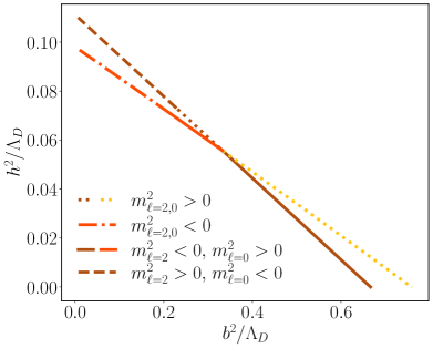
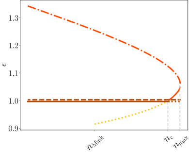
Figure 3: Two branches of solutions to (49) in the $(b^{2}/\Lambda_{D},h^{2}/\Lambda_{D})$ (left) and $(\epsilon,n)$ plane (right). The brown lines represent the Freund-Rubin branch, while the yellow (oblate) and orange (prolate) lines represent the interpolation of warped solutions reconstructed numerically. The two branches intersect at $({b_{cr}}^{2}/\Lambda_{D},{h_{cr}}^{2}/\Lambda_{D})=(0.36,0.052)$. The linestyle reflects the perturbatively unstable modes for the two branches. See figure 1 for more details.

2.4.1 Stability

The spectrum for scalar perturbations of the warped solutions was studied in Kinoshita:2009hh . Computing the eigenspectrum in a similar way to the Freund-Rubin solutions, one finds that the marginal stability of the warped solutions coincides with the marginal stability of the Freund-Rubin branch. In particular, for the $\ell=2$ mode, when $h^{2}$ satisfies the first inequality given by eq. (45), then the eigenvalue of the warped branch is positive, while the eigenvalue of the Freund-Rubin solution becomes negative. In other words, in the low Hubble regime, where the Freund-Rubin branch is unstable to inhomogeneous excitations, the warped branch is perturbatively stable. Conversely, the warped branch is unstable to inhomogeneous perturbations in the regime where the Freund-Rubin branch is stable. Additionally, the mass squared of the warped branch is larger than that of the symmetric branch in the regime where the latter is unstable, which in turn implies that the warping of the internal compact space stabilizes the shape mode of the compact space.

Alternatively, one can use a thermodynamic argument. Recall that the entropy is defined by eq. (19), where $H$ is defined by the cosmological apparent horizon (see appendix A for an explicit derivation for the warped metric ansatz). As shown in Kinoshita:2009hh , the thermodynamic stability of these solutions agrees with their dynamical stability. In other words, when $n_{c}<n<n_{\mathrm{max}}$, where $n_{c}=32\sqrt{3}\pi^{2}/\Lambda_{8}^{3/2}=0.97n_{\rm max}$, the small volume Freund-Rubin branch has a smaller Hubble parameter, or larger entropy (area), and hence is thermodynamically preferred. On the other hand, when $n<n_{c}$, the warped branch has smaller Hubble or larger entropy and is thermodynamically preferred. This is shown in figure 1. At the linear level, the dynamical and thermodynamic stability of the Freund-Rubin solutions determine the shape and stability of the warped solutions. Reference Dahlen:2014 sketched an effective potential that neatly encapsulates this behaviour. In the effective theory described by eq. 36, only the radius of the solution is treated as a dynamical radion field. If we now allow the shape of the compact space to vary as well, we must treat the aspect ratio as a dynamical field, and extend the effective potential to be a function of $L$ and $\epsilon$. Minima of the potential in the $L$ direction are now minima or maxima in the $\epsilon$ direction depending on whether the solution is stable or unstable to shape fluctuations which in turn depends on its conserved flux number. Reference Dahlen:2014 argued that this effective potential is captured by a cubic potential schematically drawn in figure (2), and that the effective potential asymptotes to $V\rightarrow+\infty$ in the oblate direction and $V\rightarrow-\infty$ in the prolate direction. Intuitively, one would expect that in the direction of decreasing $\epsilon$, the equatorial radius is increasing, and flux is concentrating there such that the solution eventually settles to a minimum. On the other hand, as $\epsilon$ increases, the equatorial radius will decrease and the flux concentrates at the poles. Having no flux to support the equator, the sphere collapses to zero radius and the potential (36) tends to $V\rightarrow-\infty$. What happens to the solution as it rolls down the potential is unclear. In the next section, we verify this general picture nonlinearly and study the endpoint of the solutions. The evolution and endpoints of the unstable solutions are summarized in figure 1.

3 Numerical implementation

We evolve the Einstein equations using the generalized harmonic formulation Garfinkle:2001ni ; Pretorius:2005 , where the gauge degrees are specified by choosing the source functions which determine the covariant d’Alembertian of the coordinates, $H^{M}=\Box x^{M}$. We choose our evolution variables according to a space-time decomposition of the metric. See appendix B for the evolution variables and equations of motion.

To numerically evolve the system, we discretize in time and $\theta$. To avoid solving the equations directly on the poles we use a shifted grid

$$\theta_{j}=\frac{j+1/2}{N_{\theta}}\pi,\qquad j=0,\ 1,\dots,\ N_{\theta}-1\ .$$ (52)

We expand the evolution variables as a sum of sines or cosines, depending on the parity of the function around the pole, and use pseudospectral methods to calculate the spatial derivatives. The variables are evolved in time using fourth-order Runge-Kutta time stepping. High-frequency spectral noise is reduced by applying an exponential filter Majda7511 . This filter is applied to the coefficients of every derivative function and directly to the coefficients of the solution at the end of each time step. The coordinate freedom is fixed by choosing the source functions. These are set to be such that the shift is driven to zero and the lapse remains approximately constant when the solution remains close to the background solution. This avoids extra dynamics coming solely from gauge transitions (as opposed to physical instability).

During the evolution, we search for, and in some cases find, trapped regions: points where both (i.e. the nominally “inward" and “outward") null geodesics moving in the $\theta$ direction must have the same sign for the derivative with respect to the affine parameter $d\theta/d\lambda$. In such cases, we excise a causally disconnected region bounded by such a point where the null geodesics are both ingoing, and instead use fourth order finite difference stencils to calculate derivatives, and Kreiss-Oliger dissipation to reduce the high-frequency noise Kreiss . In this way, we continue to evolve the spacetime outside the trapped regions.

We construct initial data describing perturbed Freund-Rubin or stationary warped solutions. To do this, we take the background metric on the initial time slice and add the perturbation given by eq. (37) with some specified amplitude. We then solve for the initial electric and magnetic forms using the Hamiltonian and momentum constraints (hence our perturbed solutions still exactly satisfy the constraints). This procedure gives rise to a slightly perturbed flux number, although close enough to background value to not affect the properties relevant for assessing stability. See appendix C for results illustrating that we start with sufficiently small perturbations so as to be in the linear instability regime, as well as numerical convergence.

In the case where the background solution is a warped solution, we construct the background solution using the procedure described in section 2.4. Note that most of the solutions presented below are for $q=4$, where only the $\ell=0$ or $\ell=2$ modes can be perturbatively unstable. We therefore only consider $\ell=0$ or $\ell=2$ perturbations, leaving the investigation higher modes in solutions with more dimensions for future work.

4 Results

We now present our numerical solutions, restricting to $p=4$ to make contact with cosmology.

4.1 Total volume instability of Freund-Rubin solutions

We begin with a discussion of the total volume instability, which affects Freund-Rubin solutions on the large volume branch. We obtain results similar to ref. Krishnan:2005 , which studied the cases where the dimensionality of the $q$-sphere was two or three. In those cases, the homogeneous mode is the only one excited, and hence the inhomogeneous perturbations ($\ell>0$) can be set to zero. Here, our initial conditions are Freund-Rubin solutions on the large volume branch in theories with $q=4$. Note that for $q=4$, the small volume branch is vulnerable to the warped instability, but the large volume branch is not. This guarantees that, at least initially, time evolution does not break the spherical symmetry of the compact space.

In the absence of the warped instability, we can understand the time evolution entirely from the perspective of the four dimensional effective theory (see appendix A for further details): Einstein gravity with a scalar field describing the radius of the compact sphere that evolves in the potential depicted in figure 2. Our initial condition lies at the maximum of the effective potential, and the evolution will take the solution either to the potential minimum (corresponding to the $dS_{p}\times S_{q}$ solution on the small-volume branch) or to a solution that decompactifies to $D=p+q$ dimensional de Sitter space.

We find that the results of the full nonlinear evolution away from the large volume Freund-Rubin solutions are as expected from the four dimensional effective theory. A small positive perturbation to the total volume leads to decompactification while a small negative perturbation evolves toward the stable small-volume $dS_{p}\times S_{q}$ solution. For the solutions that decompactify, we confirm that the curvature scalar asymptotes to what is expected for $D=p+q$ dimensional de Sitter space with a cosmological constant $\Lambda_{D}$, i.e.

$${}^{(D)}R=\frac{2D\Lambda_{D}}{D-2}\ .$$ (53)

The evolution does not lead to any significant growth away from homogeneity as the solution decompactifies, as expected based on the absence of the perturbative warped instability on the large volume branch.

For a negative total volume perturbation, the solution eventually settles to the small volume $dS_{p}\times S_{q}$ solution with the same conserved flux $n$ as the initial condition. This end state has slightly smaller radius and a slightly lower Hubble parameter (as computed from eq. (20)) compared to the initial large volume Freund Rubin solution. In the left panel of figure 4, we show the Hubble parameter as a function of the proper time at the equator, defined by $d\tau=\alpha(t,\theta=\pi/2)dt$ (though here the solutions remain homogeneous and the value of $\theta$ is irrelevant), where it can be seen that the evolution smoothly connects the large and small volume solutions. A cosmological observer in four dimensions would observe a brief period of quasi-de Sitter expansion, followed by pure de Sitter evolution. In the center and right panels of figure 4, we plot the slow-roll parameters defined by:

$$\epsilon_{\rm sl}\equiv-\frac{1}{H^{2}}\frac{dH}{d\tau_{\rm eq}},\ \ \ \ \eta_{\rm sl}\equiv\epsilon_{\rm sl}-\frac{1}{2H\epsilon_{sl}}\frac{d\epsilon_{\rm sl}}{d\tau_{\rm eq}}\ .$$ (54)

Both remain less than one over the duration of $N=H_{0}\tau_{\rm eq}\sim 5$ e-folds. This implies that the transition from the large to the small-volume branch describes a short bout of slow-roll inflation. The evolution described here therefore serves as a toy model of inflation as driven by the volume modulus of a compactification. Solutions for other choices of the flux $n$ are qualitatively similar.

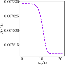
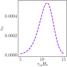
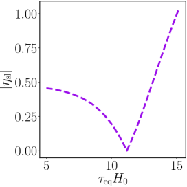
Figure 4: Sample solution on the large volume branch with $p=q=4$, $\Lambda_{D}=1,H_{0}/M_{4}=0.0078$ and an initial $\ell=0$ perturbation. Left: The effective Hubble rate, $H/M_{4}$, flows to the solution with the same value of $n$ on the small volume branch. The slow roll parameters $\epsilon_{\mathrm{sl}}$ (middle) and $\eta_{\mathrm{sl}}$ (right) during the transition. All plots are shown as a function of proper time (in particular as measured at $\theta=\pi/2$, though here the solutions remain homogeneous).

4.2 Warped instability of Freund-Rubin solutions

We now move on to study perturbations that excite the warped instability of Freund-Rubin solutions on the small volume branch. Recall that the small volume solutions are stable to the total volume instability (in the four dimensional effective theory they sit at a minimum of the effective potential), but when $q\geq 4$ they may be vulnerable to the warped instability. We focus on the case where an $8$-dimensional spacetime is compactified down to four dimensions, and the internal manifold has the topology of a $4$-sphere. This is an interesting scenario because, as we saw in Sec. 2.3.2, it features both a window of stability $n_{c}<n<n_{\rm max}$ in the range of fluxes allowed by eqs. (40) and (44), as well as perturbatively unstable solutions for $n<n_{c}$. For initial conditions, we start from a small volume Freund-Rubin solution with an $\ell=2$ perturbation; this is the only unstable mode in the linear regime.

4.2.1 Linearly stable solutions: $n_{c}<n<n_{\rm max}$

We first explore the range of fluxes $n_{c}<n<n_{\rm max}$ where the Freund-Rubin solution is linearly stable to both homogeneous and inhomogeneous perturbations. Although sufficiently small perturbations should decay, we can ask what will happen if one adds a sufficiently large homogeneous ($\ell=0$) or inhomogeneous ($\ell=2$) perturbation of the form given by eq. (37). In particular, appealing to the effective potential picture, it is not hard to imagine that the solution, originally sitting at the minimum of the potential well, will be kicked out, provided the perturbation is sufficiently large.

For large $\ell=0$ perturbations, we expect the solution to reach the maximum of the effective potential after which it will decompactify. Indeed we find that when the size of the perturbation is such that the initial volume of the perturbed solution exceeds its large volume value it will decompactify.

In the effective potential depicted in the right panel of figure 2, one can think of the potential maximum as corresponding to the stationary but unstable prolate solution on the warped branch with the same value of the conserved flux $n$ as the small-volume Freund-Rubin solution. Adding $\ell=2$ perturbations of increasing size, one eventually approaches a configuration close to this unstable prolate solution. Once the size of the perturbation exceeds this point, we expect the solution to become increasingly prolate. However, since the effective potential for the aspect ratio $\epsilon$ is only qualitative, we do not have a concrete prediction for the end-state. Likewise, with no stable warped solution to flow to, thermodynamic arguments are not of much help in determining the end-state. Note that we still put in an initial perturbation to the metric of the form given by eq. (37) (but with nonlinear corrections to the $q$-form through the constraints, as described in section ), even as we consider large perturbations beyond the linear regime.

In figure 5, we show the evolution of the aspect ratio for a stable Freund-Rubin solution when perturbed with successively larger $\ell=2$ perturbations. As expected, perturbations given by eq. (37) with sufficiently small $h$ decay. However, there is a critical initial amplitude above which the solution evolves to become more and more prolate. As this threshold is approached (around $\bar{h}\sim 0.2$), the instability timescale (after a brief transient where the aspect ratio undergoes a few damped oscillations) increases—consistent with the initial condition approaching a maximum in the effective potential. Beyond the threshold, as the compactification becomes increasingly prolate, the compactified (but not uncompactified) volume rapidly decreases, as can be seen in figure 5. By adding higher numerical resolution, we can reach higher aspect ratios and smaller compactified volumes (which have higher magnitudes of the scalar curvature) before the evolution breaks down, but at all resolutions we see no evidence that the solution is asymptoting to some non-singular state. As we will see below, this behaviour seems to be generic for solutions where the internal space becomes prolate. Note that as the prolate solutions evolve to their ultimately singular end, the four dimensional effective theory, and the effective potential depicted in figure 2 eventually are no longer valid. The effective potential in the prolate direction is therefore only indicative of the general direction of evolution.

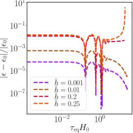
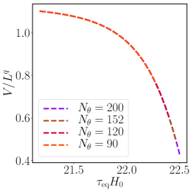
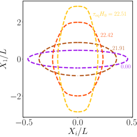
Figure 5: A sample solution on the small volume branch with $p=q=4$, $\Lambda_{D}=1$, $H_{0}/M_{4}=0.0077$ and an $\ell=2$ perturbation. Left: The relative difference between the aspect ratio of the sample solution and the background Freund-Rubin solution for successively larger perturbations. Middle: The $q$-dimensional volume of the internal space for successively higher resolutions for initial data with $(\ell,\bar{h})=(2,0.3)$. Right: Several snapshots of the embedding of internal space for initial data with $(\ell,\bar{h})=(2,0.3)$.

4.2.2 Linearly unstable solutions: $n<n_{c}$

We now discuss the evolution of Freund-Rubin solutions that are linearly unstable to $\ell=2$ perturbations, which have a flux less than the critical value $n<n_{c}$. As illustrated in figure 1, and outlined in the previous sections, at each flux $n_{\rm Mink}<n<n_{c}$ there exists a linearly unstable Freund-Rubin solution, as well as a corresponding linearly stable oblate warped solution with the same flux. The warped solution being thermodynamically preferred (e.g. with a higher entropy/lower Hubble parameter), these solutions are a natural candidate for the end point of the instability Kinoshita:2009hh ; Dahlen:2014 . This expectation is reflected in the effective potential for the aspect ratio sketched in the middle panel of figure 2. The Freund-Rubin solution is at the maximum of the effective potential, and a negative $\ell=2$ perturbation would cause the solution to evolve towards the oblate warped solution at the potential minimum. Sampling initial conditions with a wide range of fluxes, we find that the endpoint of the $\ell=2$ Freund-Rubin instability (in the $-\epsilon$ direction) is in most cases the stable warped solution with corresponding flux. The notable exceptions occur in a window of flux between $n_{\rm Mink}<n<n_{I}=435.56$, where the end state is instead a crunching prolate solution. We discuss these solutions in more detail below. The confirmation of the thermodynamic arguments in previous literature, with interesting exceptions, is one of our primary results.

To explicitly verify that the endpoints of the Freund-Rubin instability are indeed the stable warped solutions, in figure 6 we show the volume of the compact space (left) and the aspect ratio (middle) of the numerical solutions at late times (dots) compared to the corresponding quantities for the warped solutions (dashed line) from section 2.4. The agreement is excellent. Note that the warped solutions have roughly the same internal volume as the symmetric solution they evolve from. In figure 6, we also plot the instability timescale measured from the linear regime of the numerical evolution, which grows as the flux is increased. We can understand this as follows. The Hubble parameter for the Freund-Rubin and warped solution match at $n_{c}$. Therefore, as $n$ increases, the extrema of the effective potential in the $\epsilon$ direction merge, and the curvature at the maximum goes to zero—we therefore expect an increasing instability timescale as $n\rightarrow n_{c}$.

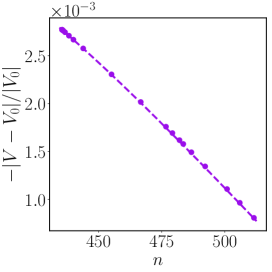
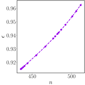
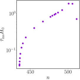
Figure 6: The volume (left), aspect ratio (middle) and ratio of instability timescale to e-fold period (right) of warped solutions with $n_{I}<n<n_{c}$ on the small volume branch for the special case $p=q=4$. We find that in this regime each unstable symmetric solution evolves to an ellipsoidal solution with $\epsilon<1$, which has roughly the same internal volume but lower effective potential. The dashed lines represent the interpolation of stationary solutions constructed as described in section 2.4, while the dots represent the end states of evolving a symmetric solution with an $\ell=2$ perturbation. For the aspect ratio, the maximum of the difference is $\sim 10^{-4}$.

We now focus on the specific example shown in figure 7 to illustrate the transition between an initially unstable spherical solution and its endpoint, a stable oblate solution. In the left panel we show the entropy, which increases monotonically as expected. There are interesting step-like features in the evolution which persist at increasing resolution, and are therefore not likely to be numerical artifacts. In the middle panel we show the Hubble parameter, which decreases monotonically over the course of $\sim 5$ e-folds to its asymptotic value. We show the embedding of the compact space in the right panel. Note that the flux is distributed on the ellipsoid the way you would expect it from the linear analysis. We found in section 2.3.2 that the unstable mode has inversely correlated flux $\bar{a}$ and shape $\bar{h}$ components, and similarly we find that whenever the radius gets larger, the flux density does too, such that, for an oblate solution, the flux is concentrated around the equator. This makes intuitive sense, as a region of larger radius implies higher curvature, and hence a larger flux density to support the region against collapse.

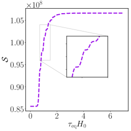
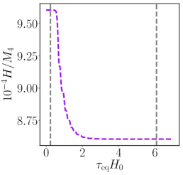
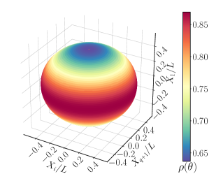
Figure 7: A sample solution on the small volume branch with $p=q=4$, $\Lambda_{D}=1$, $H_{0}/M_{4}=0.00096$, $n=436.13$ and an initial $\ell=2$ perturbation. Left: The effective entropy which is increasing between the two stationary solutions. Middle: The effective four-dimensional Hubble rate eq. (20), with grey lines indicating the approximate initial and final times of the transition period, as defined in the text. Right: The three dimensional projection of the embedding of internal space at $\tau_{\mathrm{eq}}H_{0}=8.6$. The color shows the flux density.

For the choice of flux in figure 7, the transition between the spherical and oblate solution occurs over the span of $\sim 5$ e-folds. As noted above, the instability timescale increases with $n$. Therefore, an interesting question is whether the transition period can persist over a larger number of e-folds. In this case, the four-dimensional effective theory includes a period of slow-roll leading to an asymptotic regime of pure de Sitter expansion . In figure 8, we show the maximum value that the slow-roll parameter $\epsilon_{\rm sl}$ (defined in eq. 54) takes during the evolution (left) as well as the elapsed number of e-folds during the transition. To be more precise, we define the number of e-folds between the initial ($i$) Freund-Rubin and final ($f$) stationary warped solution as $N=\int^{f}_{i}H\ d\tau_{\rm eq}$, where the time at which the slow-roll period starts (ends) is defined as when the Hubble factor differs by $10^{-4}$ relative to its initial (final) value (indicated by grey dashed lines in figure 7). We see that it is possible to get $\sim 10$–$100$ e-folds of slow-roll inflation as $n\rightarrow n_{c}$. We conclude that the evolution of unstable Freund-Rubin solutions provides a viable toy model for slow-roll inflation in flux compactifications. One interesting application of these solutions is to use the full higher dimensional picture to explicitly compute the effect of extra dimensions on the spectrum of linear scalar and tensor perturbations. This would make contact with phenomenology and cosmological observables such as the cosmic microwave background. We defer this and other possible explorations to future work.

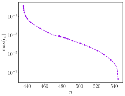
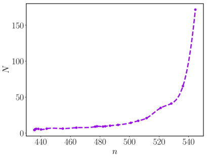
Figure 8: For unstable Freund-Rubin solutions with $n_{I}<n<n_{c}$ we plot the maximum value the slow-roll parameter $\epsilon_{\rm sl}$ takes during the evolution (left) and the number of e-folds of expansion in the four-dimensional effective theory elapsed during the transition to the stable warped end-point (right).

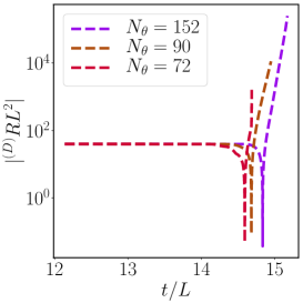
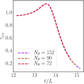
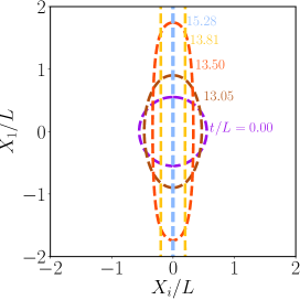
Figure 9: End state of solution on small volume Freund-Rubin branch with $p=q=4$, $\Lambda_{D}=1$, $n=n_{\text{Mink}}$ and an initial $\ell=2$ perturbation for different resolutions. The $D$-dimensional curvature scalar which becomes negative at the end (left), scale factor at the equator (middle) and embedding of internal space (right).

So far, the linear analysis has been very good at predicting what happens in the full nonlinear case. But this is not always true. In the range of flux $n_{\rm mink}<n<n_{I}=435.56$ we find that while the solution does transition to the corresponding oblate solution briefly, but does not settle there. Rather, it oscillates between the oblate and nearly spherical solution before running away to prolate values. In figure 9, we illustrate this behaviour for a limiting case where the external spacetime is Minkowski. There it can be seen that after a brief period where the internal space is oblate, the solution transitions to being more and more elongated, with the flux concentrating around the poles. In this case (in contrast to the prolate solutions discussed above), we find regions where the characteristics are ingoing, which allows us to excise a region around the poles and continue the evolution. We find that the spacetime curvature blows up, and the scale factor and equatorial circumference both tend to zero, consistent with a crunch.

Note that for the Minkowski spacetime, there are no oblate solutions with the same value of $n$, so it is not surprising that the solution goes prolate. However other solutions with $n_{\mathrm{mink}}<n<n_{I}$ have a solution on the oblate branch, and yet show the same behaviour as the Minkowski solution. We can understand this as follows. First, recall from figure 6 that as $n$ is decreased to approach $n_{I}$, the instability timescale decreases. Hence, in the language of the effective potential picture, the velocity approaching the minimum of potential will be larger, and there will be a greater tendency to overshoot, and, due to nonlinear effects, eventually roll back up the potential towards larger $\epsilon$. The smaller the flux, the shorter the timescale of instability, and we observe that solutions undergo fewer oscillations about the oblate solution as the flux is decreased. The Hubble parameter decreases monotonically, passing through zero as the solutions roll back up the potential to increasing $\epsilon$. As $H$ goes through zero, the expanding marginally inner trapped cosmological horizon becomes infinite and disappears, and a marginally outer trapped horizon appears and begins contracting. Again, this is consistent with a crunch.

To further probe the validity of the effective potential picture, we consider perturbations around initially oblate solutions in this flux range. As shown in the right panel of figure 10, small perturbations decay (consistent with the linear stability), but modestly larger perturbations cause the solution to become prolate, undergoing the same fate as the corresponding initially spherical solutions. This implies the existence of a potential barrier about the oblate solutions.

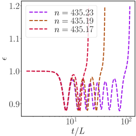
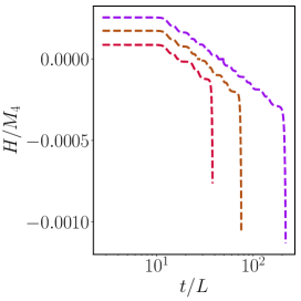
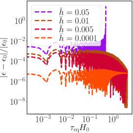
Figure 10: The aspect ratio (left) and effective Hubble rate (middle) for a few initially spherical solutions with $n<n_{I}$. The relative difference in the aspect ratio from the background value for a sample solution on the small Hubble warped branch with $p=q=4$, $\Lambda_{D}=1$ and $H_{0}/M_{4}=1.3\times 10^{-5}$ and successively larger $\ell=2$ perturbations (right).

Finally, we study initially prolate solutions to determine their fate. We expect that, in the range of flux where there is a corresponding solution on the small volume branch, they will undergo the same fate as the solutions that started out spherical or oblate but were kicked out the potential well. The left and middle panels of figure 11 show two such solutions, which indeed become extremely prolate as the equatorial radius shrinks to zero. Another interesting regime is the one with $n<n_{\mathrm{Mink}}$. As one can see from figure 1, these solutions do not have a Freund-Rubin solution they could have flowed from, hence they are distinct from the evolutions considered so far. The right panel of figure 11 shows the embedding of the compact space for such a solution. Those solutions become not only very oblate but also extremely large in volume. Around the equator, the flux density approaches zero, and the expansion rate approaches that expected from the decompactified $D$-dimensional de Sitter solution. However, the internal space remains very inhomogeneous. We are unable to continue the evolution indefinitely, as tracking the distorted shape and differing expansion rates requires higher and higher numerical resolution. However, we do not find any singular behaviour before then. This distorted shape is qualitatively different from any of the solutions considered above.

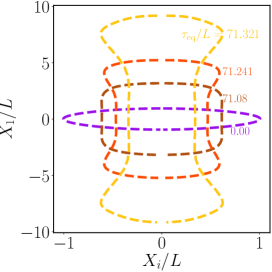
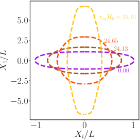
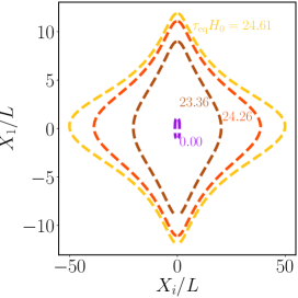
Figure 11: Sample solutions on the large Hubble warped branch with $p=q=4$, $\Lambda_{D}=1,\left(H_{0}/M_{4},n\right)=(1.3\times 10^{-5},435.23)$ (left), $\left(H_{0}/M_{4},n\right)=(0.0077,529.29)$ (middle) and $\left(H_{0}/M_{4},n\right)=(0.0075,402.11)$ (right) where recall $n_{\rm Mink}=435.16$.

Finally, we briefly report on higher dimensional spaces where $q\geq 5$. Exploring a few cases with $q=5$, we find similar behaviour to the case where $q=4$. In particular, we find a range of flux where the Freund-Rubin solution is only unstable to the total volume instability, and another where it is unstable to the warped instability only. In the latter case, we again find a range of the parameter space where the unstable solutions flow towards stable stationary oblate solutions, but outside that range the solutions will, in a similar way to the solutions shown in figure 9, become increasingly prolate forming trapped regions in the process and eventually crunching. However, it is important to note that for $q\geq 5$, the range of the inequalities in eqs. (40) and (44) overlap, and hence none of the Freund-Rubin solutions are stable. For future work, it would thus be interesting to see which instability dominates in this overlap region of the parameter space. Additionally, in contrast to $q=4$, when $q\geq 5$, higher $\ell$ modes can be unstable, which in theory would result into further breaking of the symmetry of the compact sphere.

5 Conclusions

Despite extensive study of the linear stability and mass spectrum of Freund-Rubin like solutions, very little is known about their nonlinear evolution and dynamical formation. In this work we have explored how such solutions might be generated and evolve. The starting point for this flux compactification scenario was the product space of a $p$-dimensional de Sitter space and a $q$-dimensional (in some cases warped) topological sphere. Provided we fix the higher dimensional constant $\Lambda_{D}$ and the dimension of the internal manifold, the properties and stability of the $p$-dimensional vacua and the compact space, will depend on the number of flux units of the $q$-form field strength wrapping the sphere or the Hubble parameter of the extended dimensions. For each value of the conserved flux number $n<n_{\mathrm{max}}$ there are four solutions. Homogeneous solutions can be classified into two branches, a large volume branch, unstable to the $\ell=0$ scalar sector and a small volume branch unstable to the $\ell=2$ mode for $n<n_{c}<n_{\mathrm{max}}$. On the stationary warped branch one finds the so-called large Hubble branch, unstable to the $\ell=2$ mode for $n<n_{\mathrm{max}}$, and the small Hubble warped branch which is stable to the $\ell=2$ mode for $n<n_{c}$ but unstable for $n_{c}<n<n_{\mathrm{max}}$.

To gain some understanding of the parameter space and dynamics, we studied the evolution of initially small perturbations around those stationary solutions. We find, in agreement with previous studies that, for any dimensionality of the sphere, solutions on the large volume branch either decompactify to empty $D$-dimensional de Sitter space with cosmological constant $\Lambda_{D}$ or flow to the solution on the small volume branch with the same number of flux units but a smaller volume, and hence large enough flux density to stabilize the sphere against collapse.

We show that within the regime where the small volume Freund-Rubin solution is unstable to the $\ell=2$ scalar mode, when $n_{I}<n<n_{c}$ the solutions flow to the corresponding solution on the small Hubble warped branch. The end point of the instability is a stationary oblate solution where the flux is concentrated in a band around the equator. We do not find any other instabilities and conclude this is the final endpoint of the solution, at least under our symmetry assumptions. However, for $n<n_{I}$, but still within the regime where the small volume Freund-Rubin branch is unstable, we find that the solution overshoots the linearly stable oblate solution, flowing towards an increasing prolate solution, where the flux concentrates at the poles of the sphere. The equator of the $q$-sphere is unsupported by flux, and the equatorial radius shrinks to zero size in finite time, forming trapped regions around the poles in the process. The four-dimensional spacetime undergoes a crunch.

Finally, regarding the end state of solutions on the large Hubble branch with $n<n_{\mathrm{Mink}}$, we find that the volume of the internal space grows, while the shape become increasingly oblate, but with cuspy feature at the poles. The expansion rate remains inhomogeneous, as there is no solution on the small Hubble branch with the same number of flux units.

It follows from the above that the warping of the compact space may stabilize initially unstable configurations. This spontaneous symmetry breaking of the internal space to more dynamically favoured configurations is a very natural phenomenon in cosmology. In the case of the Jeans instability, configurations with high mass density suffer from a gravitational instability. This symmetry breaking instability is ultimately cut-off by nonlinear terms leading to structure formation. Other analogous examples include the Gregory-Laflamme instability Gregory:1994bj .

There are a number of directions in which one could expand on this study. While here we assumed that only one of the spatial degrees of freedom in the internal space were excited, it would be interesting to allow additional symmetries either in the compactified, or uncompactified dimensions, to be broken. Another possible avenue would be to study the case where the external space is anti-de Sitter, with potential applications to the AdS/CFT correspondence. Here, we have focused on a simple model in order to gain insight into open questions surrounding extra dimensions and spherical compactifications. For example, there has been much debate and conjecture regarding the circumstances under which it is possible to have periods of exponential expansion in compactified scenarios Cicoli:2018kdo ; Palti:2019pca . The general methods presented here could be used to explore this issue in scenarios that are dynamical and inhomogeneous.

Appendix A Dimensional reduction

In this section, we illustrate the properties of dimensional reduction with several examples. Recall that in our units $M_{D}\equiv(8\pi G_{D})^{-1/(D-2)}=1$.

A.1 Time-dependent Freund-Rubin Solution

We start with a simple example, where identifying scale factor and moduli fields in the four-dimensional effective theory is straightforward. Consider solutions of the form:

$$ds^{2}=-\alpha(t)^{2}dt^{2}+a(t)^{2}d\vec{x}_{p-1}^{2}+L(t)^{2}d\Omega_{q}^{2}\ .$$ (55)

This metric ansatz encompasses the static Freund-Rubin solutions of section 2.3, as well as the time-dependent solutions resulting from total-volume ($\ell=0$) perturbations of the static Freund-Rubin solutions. For such solutions, we have

$$\frac{K-{K^{x}}_{x}}{2} = \frac{\dot{a}}{\alpha a}+\frac{q}{2}\frac{\dot{L}}{\alpha L}\ .$$ (56)

Defining

$$\tilde{\alpha}=\left(L/L_{0}\right)^{q/2}\alpha,\ \ \ \tilde{a}=\left(L/L_{0}\right)^{q/2}a\ ,$$ (57)

where $L_{0}\equiv L(t=0)$ we have that

$$\int d^{q}y\sqrt{\gamma_{q}}\alpha\gamma_{xx}^{3/2}\left(\frac{{K^{x}}_{x}-K}{2}\right)^{2}=\left(L_{0}^{q}\int d\Omega_{q}\right)\tilde{\alpha}\tilde{a}^{3}\left(\frac{\dot{\tilde{a}}}{\tilde{\alpha}\tilde{a}}\right)^{2}\ .$$ (58)

From this expression we can identify $\tilde{\alpha}$ as the four dimensional lapse, $\tilde{a}$ as the four dimensional scale factor and therefore:

$$M_{4}^{2}=L_{0}^{q}\int d\Omega_{q},\ \ \ \sqrt{-g(t)}=\tilde{\alpha}\tilde{a}^{3},\ \ \ H^{2}=\left(\frac{\dot{\tilde{a}}}{\tilde{\alpha}\tilde{a}}\right)^{2}\ .$$ (59)

Note that the change of variables defined by eq. (57) is precisely the conformal transformation of the four-dimensional metric that brings us to the four-dimensional Einstein frame (e.g. the conformal frame in which the Planck mass is constant in time); for comparison, see, e.g., refs. Carroll:2009dn ; Dahlen:2014 .

Evaluating the area of the cosmological apparent horizon using eq. (17), we obtain:

$$\mathcal{A}_{H} = 4\pi\int d\Omega_{q}L_{0}^{q}\left(\frac{\tilde{\alpha}\tilde{a}}{\dot{\tilde{a}}}\right)^{2}=M_{4}^{2}\frac{4\pi}{H^{2}}\ .$$ (60)

The entropy, eq. (19), is given by $\mathcal{S}=16\pi M_{4}^{2}/H^{2}$, which is the value one would have assigned based purely on the four dimensional effective theory.

For the time-dependent Freund-Rubin solutions, it is possible to derive the full dimensionally reduced action. This can be found, e.g., in refs. Carroll:2009dn ; Dahlen:2014 , which we reproduce here for completeness. Expanding the terms in the action we obtain

$$S = \frac{1}{2}\int d^{4}xd^{q}y\ \sqrt{-g}\left[-6\left(\frac{{K^{x}}_{x}-K}{2}\right)^{2}\right.$$

$$+ \frac{1}{2}({K^{\theta}}_{\theta})^{2}+\frac{(q+3)(q-1)}{4}({K^{\phi}}_{\phi})^{2}+({K^{\theta}}_{\theta}+\frac{q-1}{2}{K^{\phi}}_{\phi})^{2}$$

$$+ \left.{}^{(D-1)}R-2\Lambda_{D}-\frac{1}{q!}\mathbf{F}_{q}^{2}\right]\ .$$

Evaluating the various terms in the action for the metric ansatz eq. (55) we have:

$$\frac{1}{2}({K^{\theta}}_{\theta})^{2}+\frac{(q+3)(q-1)}{4}({K^{\phi}}_{\phi})^{2}+({K^{\theta}}_{\theta}+\frac{q-1}{2}{K^{\phi}}_{\phi})^{2}=\frac{q(q+2)}{2}\left(\frac{\dot{L}}{L}\right)^{2}\ ,$$ (62)

$${}^{(D-1)}R=\frac{q(q-1)}{L^{2}}$$ (63)

and

$$\frac{1}{q!}\mathbf{F}_{q}^{2}=\frac{Q_{B}^{2}}{L^{2q}}=\frac{1}{M_{4}^{4}}\frac{n^{2}}{L^{2q}}\ .$$ (64)

Using the relations eqs. (57) and (59), we have

$$S = \int d^{4}x\ \tilde{\alpha}\tilde{a}^{3}\left[-\frac{M_{4}^{2}}{2}6H^{2}+\frac{M_{4}^{2}}{2}\frac{L_{0}^{q}q(q-1)}{2L^{q+2}}\dot{L}^{2}-V(L)\right]$$ (65)

where we have defined the effective potential

$$\frac{V(L)}{M^{4}_{4}}\equiv\frac{1}{2}\left(\frac{L_{0}}{L}\right)^{q}\left(-\frac{q(q-1)}{L^{2}}+2\Lambda_{D}+\frac{1}{M_{4}^{4}}\frac{n^{2}}{L^{2q}}\right)\ .$$ (66)

We see that the dimensionally-reduced theory is that of an FLRW Universe with a scalar field $L$ (with a non-canonical kinetic term) evolving in the effective potential $V(L)$ (plotted in figure 2).

A.2 Factorizable warped metrics

Another illustrative example is given by solutions of the form:

$$ds^{2} = e^{2A(y,t)}\left[-\left(\alpha(t)^{2}-e^{-\frac{2(q+2)}{(q-2)}A(y,t)}\tilde{g}_{\gamma\delta}\beta^{\gamma}(y,t)\beta^{\delta}(y,t)\right)dt^{2}+a(t)^{2}d\vec{x}_{p-1}^{2}\right]$$ (67)

$$+ 2e^{-\frac{8}{q-2}A(y,t)}\tilde{g}_{\gamma\delta}(y)\beta^{\gamma}(y,t)dtdy^{\delta}+e^{-\frac{8}{q-2}A(y,t)}\tilde{g}_{\gamma\delta}(y)dy^{\gamma}dy^{\delta}\ .$$ (68)

For $q=6$, this ansatz is characteristic of warped solutions to Type IIB string theory Giddings:2001yu ; Giddings:2005ff ; Frey:2008xw . We have that

$$\frac{K^{x}_{x}-K}{2} = \frac{e^{-A}}{\alpha}\left(\frac{\dot{a}}{a}-\frac{q+2}{q-2}\partial_{0}{A}-\frac{1}{4}\tilde{g}^{\gamma\delta}\mathcal{L}_{\beta}\tilde{g}_{\gamma\delta}\right)\$$ (69)

where $\partial_{0}\equiv\partial_{t}-\mathcal{L}_{\beta}$. Defining

$$\tilde{\alpha}(y,t)=e^{-\frac{q+2}{q-2}A(y,t)}\alpha(t),\ \ \ \tilde{a}(y,t)=e^{-\frac{q+2}{q-2}A(y,t)}a(t)$$ (70)

we have

$$\int d^{q}y\sqrt{\gamma_{q}}\ \alpha\gamma_{xx}^{3/2}\left(\frac{{K^{x}}_{x}-K}{2}\right)^{2}=\int d^{q}y\sqrt{\tilde{g}}\ \tilde{\alpha}\tilde{a}^{3}\left[\left(\frac{\dot{\tilde{a}}}{\tilde{\alpha}\tilde{a}}\right)^{2}+F(\beta)\right]\ .$$ (71)

Although the change of variables proposed above allows one to decompose the action in a suggestive form, it is not immediately clear how to identify the four-dimensional Planck mass, scale factor and lapse. This is due both to the presence of terms involving the shift (written above as $F(\beta)$), as well as the average of a product of $y$-dependent factors over the compact space. The latter problem arises because eq. (70) defines a conformal transformation of the four dimensional metric that depends on both time and the coordinates on the compact space. This can be contrasted with the standard approach to dimensional reduction in the presence of warping, where one defines a purely time dependent conformal transformation to the four-dimensional metric.

Ignoring terms evolving the shift for the remainder of the calculation (i.e. setting $\beta^{\gamma}=0$ and denoting the neglected terms with an ellipsis) for simplicity, we can make contact with the standard approach as follows. First, we decompose the action as follows:

$$\sqrt{-g_{4}}M_{4}^{2}H^{2} = \int d^{q}y\sqrt{\tilde{g}}\ \alpha a^{3}\left[\frac{\dot{a}}{\alpha a}-\frac{q+2}{q-2}\frac{\dot{A}}{\alpha}+\ldots\right]^{2}e^{-2\frac{q+2}{q-2}A}$$

$$= \alpha a^{3}\left(\int d^{q}y\sqrt{\tilde{g}}\ e^{-\frac{4q}{q-2}A(y,t=0)}\right)\times$$

$$\left[\left(\frac{\dot{a}}{\alpha a}\right)^{2}e^{\phi(t)}+\left(\frac{\dot{a}}{\alpha^{2}a}\right)\frac{de^{\phi(t)}}{dt}+\left(\frac{1}{2\alpha}\frac{de^{\phi(t)}}{dt}\right)^{2}\right]+\Delta+\ldots$$

$$= \bar{\alpha}\bar{a}^{3}\left(\int d^{q}y\sqrt{\tilde{g}}e^{-\frac{4q}{q-2}A(y,t=0)}\right)\left[\frac{\dot{\bar{a}}}{\bar{\alpha}\bar{a}}\right]^{2}+\Delta+\ldots$$

where we have made the following definitions:

$$e^{\phi(t)}\equiv\frac{\int d^{q}y\sqrt{\tilde{g}}e^{-2\frac{q+2}{q-2}A}}{\int d^{q}y\sqrt{\tilde{g}}\ e^{-\frac{4q}{q-2}A(y,t=0)}}\ ,$$ (73)

and

$$\bar{\alpha}(t)\equiv\alpha(t)e^{\phi(t)/2},\ \ \ \bar{a}(t)\equiv a(t)e^{\phi(t)/2}$$ (74)

and

$$\Delta\equiv\frac{(q+2)^{2}}{(q-2)^{2}}\frac{a^{3}}{\alpha}\int d^{q}y\sqrt{\tilde{g}}\ \dot{A}e^{-2\frac{q+2}{q-2}A}\left[\dot{A}-\langle\dot{A}\rangle\right]\ ,$$ (75)

where

$$\langle\dot{A}\rangle\equiv\frac{\int d^{q}y\sqrt{\tilde{g}}\ \dot{A}e^{-2\frac{q+2}{q-2}A}}{\int d^{q}y\sqrt{\tilde{g}}}=-\frac{q-2}{2(q+2)}\frac{de^{\phi}}{dt}\ e^{-\frac{4q}{q-2}A(y,t=0)}\ .$$ (76)

To the extent that $\Delta$ is small (and again, we are neglecting terms involving the shift), we can identify

$$M_{4}^{2}=\int d^{q}y\sqrt{\tilde{g}}\ e^{-\frac{4q}{q-2}A(y,t=0)},\ \ \ \sqrt{-g_{4}}=\bar{\alpha}\bar{a}^{3},\ \ \ H^{2}=\left[\frac{\dot{\bar{a}}}{\bar{\alpha}\bar{a}}\right]^{2}\ .$$ (77)

This definition for $M_{4}$ is not the same as in previous literature Giddings:2001yu ; Giddings:2005ff ; Frey:2008xw , but rather chosen to be consistent with our convention eq. (21). Note that eq. (74) defines the conformal transformation typically used in the literature to transform to the Einstein frame.

Evaluating the cosmological apparent horizon area using eq. (17)

$$\mathcal{A}_{H} = 4\pi\int d^{q}y\sqrt{\tilde{g}}\ e^{-2\frac{q+2}{q-2}A}\left(\frac{\dot{a}}{\alpha a}-\frac{q+2}{q-2}\frac{\dot{A}}{\alpha}+\ldots\right)^{-2}\ .$$ (78)

In the case where we make the approximation that $\dot{A}\simeq\langle\dot{A}\rangle$ (and neglecting terms involving the shift) we find:

$$\mathcal{A}_{H} = 4\pi\int d^{q}y\sqrt{\tilde{g}}\ e^{-2\frac{q+2}{q-2}A}\left(\frac{\dot{\bar{a}}}{\bar{\alpha}\bar{a}}\right)^{-2}e^{-\phi}=M_{4}^{2}\frac{4\pi}{H^{2}}\ .$$ (79)

Though, for general warped metrics of the form eq. (67), the cosmological apparent horizon cannot be precisely associated with the Hubble parameter as defined by dimensional reduction in previous literature. However, we note that for the static warped solutions discussed in the text, $\dot{A}=\beta^{\gamma}=0$, and the correspondence does hold.

Appendix B $(D-1)+1$ equations

B.1 Maxwell equations

Plugging in our metric and flux ansatz into the Maxwell equations (4), the evolution equations for the electric and magnetic fluxes become

$$\begin{array}[]{lcl}\dot{Q_{E}}&=&\beta^{\theta}{Q_{E}}\bigg{(}\frac{Q_{E}^{\prime}}{Q_{E}}+(q-1)\cot\theta\bigg{)}+\alpha KQ_{E}+2\alpha(q-1)K^{\phi_{1}}_{\phi_{1}}Q_{E}-\alpha\gamma_{\theta\theta}^{-1}Q_{B}^{\prime}\vspace{0.5em}\\ &&+\alpha\gamma_{\theta\theta}^{-1}Q_{B}\bigg{(}-(p-1)\frac{\gamma_{xx}^{\prime}}{2\gamma_{xx}}+\frac{\gamma_{\theta\theta}^{\prime}}{2\gamma_{\theta\theta}}+(q-1)\frac{\widetilde{\gamma}_{\phi_{1}\phi_{1}}^{\prime}}{2\widetilde{\gamma}_{\phi_{1}\phi_{1}}}\bigg{)}-\gamma_{\theta\theta}^{-1}(\partial_{\theta}\alpha)Q_{B}\end{array}$$ (80)

and

$$\begin{array}[]{lcl}\dot{Q_{B}}&=&\beta^{\theta}Q_{B}\bigg{(}\frac{Q_{B}^{\prime}}{Q_{B}}+(q-1)\cot\theta\bigg{)}+Q_{B}\partial_{\theta}\beta^{\theta}-\alpha\left(Q_{E}^{\prime}+(q-1)Q_{E}\cot\theta\right)\vspace{1em}\\ &&-(\partial_{\theta}\alpha)Q_{E}\end{array}$$ (81)

where the dot represents differentiation with respect to time.

B.2 Generalized harmonic equations

We evolve the solutions using a space-time decomposition of the generalized harmonic formulation Garfinkle:2001ni ; Pretorius:2005 . Here we write down the field equations for completeness. In this formulation, the lapse and shift are evolution variables, in addition to the spatial metric and extrinsic curvature. We also introduce the auxiliary fields $\pi$ and $\rho^{\bar{m}}$ that are directly related to the time derivative of $\alpha$ and $\beta^{\bar{m}}$. We fix the coordinate degrees of freedom by specifying a so-called source vector, $H^{M}$ such that the constraint vector

$$C^{M}\equiv H^{M}+\left({}^{(D)}{\Gamma^{M}}_{NK}-^{(D)}{\bar{\Gamma}^{M}}_{NK}\right)g^{NK}=0$$ (82)

vanishes. Here ${}^{(D)}{\bar{\Gamma}^{M}}_{NK}$ denotes a background connection. The generalized harmonic equations are

$$\begin{array}[]{lcl}{}^{(D)}R_{MN}-\nabla_{(M}C_{N)}=-\kappa\left[n_{(M}C_{N)}-\frac{1}{(D-2)}g_{MN}n^{L}C_{L}\right]+\left[T_{MN}-\frac{1}{D-2}g_{MN}T\right]\ .\end{array}$$ (83)

These are hyperbolic, provided the source functions are specified directly as a function of the spacetime coordinates $x^{M}$ and the metric $g_{MN}$.

We evolve the $(D-1)+1$ form of the generalized harmonic evolution equations Brown:2011 as follows

$$\partial_{t}\gamma_{xx}=-2\alpha K_{xx}+\gamma_{xx}^{\prime}\beta^{\theta}$$ (84a)

$$\partial_{t}\gamma_{\theta\theta}=-2\alpha K_{\theta\theta}+2\gamma_{\theta\theta}\partial_{\theta}\beta^{\theta}+\beta^{\theta}\gamma_{\theta\theta}^{\prime}$$ (84b)

$$\partial_{t}\widetilde{\gamma}_{\phi_{1}\phi_{1}}=-2\alpha\widetilde{K}_{\phi_{1}\phi_{1}}+\beta^{\theta}(\widetilde{\gamma}_{\phi_{1}\phi_{1}}^{\prime}+2\cot\theta\widetilde{\gamma}_{\phi_{1}\phi_{1}})$$ (84c)

$$\partial_{t}K_{xx} = -\frac{\gamma_{xx}^{\prime}}{2\gamma_{\theta\theta}}\partial_{\theta}\alpha+\alpha\left({}^{(D-1)}R_{xx}-2K^{x}_{x}K_{xx}+KK_{xx}\right)+\alpha\left(\frac{1}{D-2}\gamma_{xx}(S-\rho)-S_{xx}\right)$$ (85a)

$$+\beta^{\theta}\partial_{\theta}K_{xx}-\alpha C_{\perp}K_{xx}-\alpha\frac{1}{2}\gamma_{xx}^{\prime}C^{\theta}-\kappa\alpha\gamma_{xx}C_{\perp}/2$$

$$\partial_{t}K_{\theta\theta} = -\partial^{2}_{\theta}\alpha+\frac{\gamma_{\theta\theta}^{\prime}}{2\gamma_{\theta\theta}}\partial_{\theta}\alpha+\alpha\left({}^{(D-1)}R_{\theta\theta}-2K^{\theta}_{\theta}K_{\theta\theta}+KK_{\theta\theta}\right)+\alpha\left(\frac{1}{D-2}\gamma_{\theta\theta}(S-\rho)-S_{\theta\theta}\right)$$ (85b)

$$+\beta^{\theta}\partial_{\theta}K_{\theta\theta}+2K_{\theta\theta}\partial_{\theta}\beta^{\theta}-\alpha C_{\perp}K_{\theta\theta}-\alpha\frac{1}{2}\gamma_{\theta\theta}^{\prime}C^{\theta}-\alpha\gamma_{\theta\theta}\partial_{\theta}C^{\theta}-\kappa\alpha\gamma_{\theta\theta}C_{\perp}/2$$

$$\partial_{t}\widetilde{K}_{\phi_{1}\phi_{1}} = -\left(\cot\theta\frac{\widetilde{\gamma}_{\phi_{1}\phi_{1}}}{{\gamma_{\theta\theta}}}+\frac{\widetilde{\gamma}_{\phi_{1}\phi_{1}}^{\prime}}{2\gamma_{\theta\theta}}\right)\partial_{\theta}\alpha+\alpha\left(\frac{{}^{(D-1)}R_{\phi_{1}\phi_{1}}}{\sin^{2}\theta}-2\widetilde{\gamma}^{\phi_{1}\phi_{1}}(\widetilde{K}_{\phi_{1}\phi_{1}})^{2}+K\widetilde{K}_{\phi_{1}\phi_{1}}\right)\vspace{1em}$$

$$+\frac{1}{p+q-2}\alpha\widetilde{\gamma}_{\phi_{1}\phi_{1}}\left(-2\Lambda_{D}+\widetilde{\gamma}_{\phi_{1}\phi_{1}}^{-(q-1)}(p-1)\big{[}Q_{E}^{2}-\gamma_{\theta\theta}^{-1}Q_{B}^{2}\big{]}\right)\vspace{1em}$$

$$+\left(\partial_{\theta}\widetilde{K}_{\phi_{i}\phi_{i}}-\frac{\widetilde{\gamma}_{\phi_{1}\phi_{1}}^{\prime}}{\widetilde{\gamma}_{\phi_{1}\phi_{1}}}\widetilde{K}_{\phi_{i}\phi_{i}}\right)\beta^{\theta}-\alpha C_{\perp}\widetilde{K}_{\phi_{1}\phi_{1}}-\alpha\left[\cot\theta\widetilde{\gamma}_{\phi_{1}\phi_{1}}+\frac{1}{2}\widetilde{\gamma}_{\phi_{1}\phi_{1}}^{\prime}\right]C^{\theta}-\kappa\alpha\widetilde{\gamma}_{\phi_{1}\phi_{1}}C_{\perp}/2$$

$$\partial_{t}\alpha = \alpha^{2}\pi-\alpha^{2}H_{\perp}+\beta^{\theta}\partial_{\theta}\alpha\vspace{1em}$$ (86a)

$$\partial_{t}\beta^{\theta} = \beta^{\theta}\partial_{\theta}\beta^{\theta}+\alpha^{2}\rho^{\theta}-\alpha\gamma^{\theta\theta}\partial_{\theta}\alpha+\alpha^{2}H^{\theta}$$ (86b)

and

$$\partial_{t}\pi = -\alpha\left((p-1)K_{xx}K^{xx}+K_{\theta\theta}K^{\theta\theta}+(q-1)K_{\phi_{1}\phi_{1}}K^{\phi_{1}\phi_{1}}\right)+D_{\bar{m}}D^{\bar{m}}\alpha\vspace{1em}$$ (87a)

$$+C^{\theta}\partial_{\theta}\alpha-\frac{(D-3)}{(D-2)}\kappa\alpha C_{\perp}-\alpha\frac{1}{D-2}((D-3)\rho+S)+\beta^{\theta}\partial_{\theta}\pi$$

$$\partial_{t}\rho^{\theta} = \gamma^{\bar{n}\bar{l}}\bar{D}_{\bar{n}}\bar{D}_{\bar{l}}\beta^{\bar{\theta}}+\alpha\gamma^{\theta\theta}\partial_{\theta}\pi-\pi\gamma^{\theta\theta}\partial_{\theta}\alpha-2K^{\theta\theta}\partial_{\theta}\alpha\vspace{1em}$$

$$+2\alpha\left[-(p-1)\frac{\gamma_{xx}^{\prime}}{2\gamma_{\theta\theta}}K^{xx}+\frac{\gamma_{\theta\theta}^{\prime}}{2\gamma_{\theta\theta}}K^{\theta\theta}+(q-1)\bigg{[}-(\cot\theta\frac{\widetilde{\gamma}_{\phi_{1}\phi_{1}}}{\gamma_{\theta\theta}}+\frac{\widetilde{\gamma}_{\phi_{1}\phi_{1}}^{\prime}}{2\gamma_{\theta\theta}})+\cot\theta\bigg{]}\widetilde{K}^{\phi_{1}\phi_{1}}\right]\vspace{1em}$$

$$+\kappa\alpha C^{\theta}-2\alpha j^{\theta}+(\beta^{\theta}\partial_{\theta}\rho^{\theta}-\rho^{\theta}\partial_{\theta}\beta^{\theta})+(q-1)\beta\widetilde{\gamma}_{\phi_{1}\phi_{1}}^{-1}\vspace{1em}$$

with the non-trivial constraints

$$C_{\perp}\equiv\pi+K=0$$ (88a)

$$C^{\theta} = -\rho^{\theta}-(p-1)\frac{\gamma_{xx}^{\prime}}{2\gamma_{\theta\theta}}\gamma^{xx}+\frac{\gamma_{\theta\theta}^{\prime}}{2\gamma_{\theta\theta}}\gamma^{\theta\theta}=0$$ (88b)

$$+(q-1)\bigg{[}-(\cot\theta\frac{\widetilde{\gamma}_{\phi_{1}\phi_{1}}}{\gamma_{\theta\theta}}+\frac{\widetilde{\gamma}_{\phi_{1}\phi_{1}}^{\prime}}{2\gamma_{\theta\theta}})+\cot\theta\bigg{]}\widetilde{\gamma}^{\phi_{1}\phi_{1}}$$

$$\mathcal{H}={}^{(D-1)}R-3K_{xx}K^{xx}-K_{\theta\theta}K^{\theta\theta}-(q-1)K_{\phi_{i}\phi_{i}}K^{\phi_{i}\phi_{i}}+K^{2}-2\rho=0$$ (88c)

$$\mathcal{M}_{\theta} = D_{\bar{m}}{K^{\bar{m}}}_{\theta}-D_{\theta}K-j_{\theta}=0$$ (88d)

where $K\equiv\gamma^{\bar{m}\bar{n}}K_{\bar{m}\bar{n}}$, ${}^{(D-1)}R=\gamma^{\bar{m}\bar{n}}R_{\bar{m}\bar{n}}$, $\bar{D}_{\bar{m}}$ denotes the covariant derivative associated with the background metric $\bar{g}_{MN}$ which we assume to have a lapse of one, shift of zero and a time-independent spatial metric under $(D-1)+1$ splitting. We also define $H_{\perp}\equiv n^{M}H_{M}$, $H^{\bar{m}}\equiv{\gamma^{\bar{m}}}_{N}H^{N}$ and the various projections of stress-energy tensor $T_{MN}$ as $S_{\bar{m}\bar{n}}=\gamma^{M}_{\bar{m}}\gamma^{N}_{\bar{n}}T_{MN}$, $\rho=n^{M}n^{N}T_{MN}$ and $j_{\bar{m}}=-\gamma^{K}_{\bar{m}}T_{KN}n^{N}$.

We find that our solutions are more stable if we choose a gauge such that the shift vector is driven to zero, and the lapse is constant in time for the stationary background solutions,

$$H^{\theta}=-\frac{\eta}{\alpha^{2}}\beta^{\theta},\ \ \ \ H^{\perp}=-K_{0}$$ (89)

where $K_{0}$ is the initial value of the trace of the extrinsic curvature and $\eta$ is some constant controlling the rate at which the shift is driven to zero. We typically set $\kappa=15$ and $\eta=10$ in units where $\Lambda_{D}=1$, although their exact values are not too important.

Appendix C Convergence tests

Ensuring that the constraints converge to zero with increasing numerical resolution, and at the expected order, provides a consistency check that the numerical solution obtained is converging to a solution of the field equations. Our numerical scheme converges at fourth order with temporal resolution and exponentially with spatial resolution. Figure (12) shows the integrated norm of the constraint violation given by eq. (82) for several resolutions, demonstrating that this quantity is converging to zero at the expected rate. The highest temporal resolution used in the resolution study is equivalent to the resolution we use for the other solutions. The spatial resolution required depends on whether the solution has inhomogeneous features that needs to be resolved or not. For homogeneous solutions we typically use $N_{\theta}\sim 20$, for stationary oblate solutions $N_{\theta}\sim 72$ and finally the prolate solutions typically require up to $N_{\theta}\sim 152$. For unstable solutions, we perturb the solutions with a sufficiently small amplitude to ensure that we are in the linear regime. In figure 12, we plot the evolution of the metric variable $\gamma_{\theta\theta}$ for a Freund-Rubin solution unstable to the warped instability, and perturbed with an initial amplitude of $\bar{h}=10^{-5}$ and $\bar{h}=5\times 10^{-5}$. Both solutions undergo a clear exponential growth phase before entering the nonlinear regime, with the time of saturation being set by the amplitude of the initial perturbation.

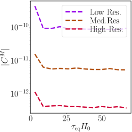
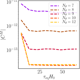
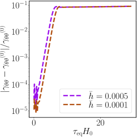
Figure 12: Integrated norm of the constraint violation eq. (82) for different temporal (left) and spatial (middle) resolutions as a function of proper time (in units of the background Hubble expansion) for $q=4$, $\Lambda_{D}=1$, $H/M_{4}=0.0078$ and an initial $\ell=2$ perturbation. The medium and high temporal resolutions have $2\times$ and $4\times$ the resolution of the low resolution run. $N_{\theta}$ in the middle indicates the number of collocation points used. We find that the constraint violations converge at fourth order in time and exponentially in space. (Right) The time evolution of spatial average of relative difference of $\gamma_{\theta\theta}$ from its background solution for $q=4$, $H/M_{4}=0.0050$ and an initial $\ell=2$ perturbation of magnitude $\bar{h}=10^{-4}$ and $\bar{h}=5\times 10^{-4}$. The linear warped instability is evident.

References

- (1) T. Kaluza, Zum Unitätsproblem der Physik, Sitzungsber. Preuss. Akad. Wiss. Berlin (Math. Phys. ) 1921 (1921) 966 [1803.08616].
- (2) O. Klein, Quantum Theory and Five-Dimensional Theory of Relativity. (In German and English), Z.Phys. 37 (1926) 895.
- (3) N. Arkani-Hamed, S. Dimopoulos and G. Dvali, The Hierarchy problem and new dimensions at a millimeter, Phys.Lett. B429 (1998) 263 [hep-ph/9803315].
- (4) L. Randall and R. Sundrum, A Large mass hierarchy from a small extra dimension, Phys.Rev.Lett. 83 (1999) 3370 [hep-ph/9905221].
- (5) L. Randall and R. Sundrum, An Alternative to compactification, Phys.Rev.Lett. 83 (1999) 4690 [hep-th/9906064].
- (6) L. Susskind, The anthropic landscape of string theory, in Universe or Multiverse, Cambridge University Press (2003).
- (7) P.G.O. Freund and M.A. Rubin, Dynamics of Dimensional Reduction, Phys. Lett. 97B (1980) 233.
- (8) R. Bousso, O. DeWolfe and R.C. Myers, Unbounded entropy in space-times with positive cosmological constant, Found. Phys. 33 (2003) 297 [0205080].
- (9) J.M. Maldacena, The Large N limit of superconformal field theories and supergravity, Int. J. Theor. Phys. 38 (1999) 1113 [hep-th/9711200].
- (10) M.R. Douglas and S. Kachru, Flux compactification, Rev. Mod. Phys. 79 (2007) 733 [hep-th/0610102].
- (11) F. Denef, M.R. Douglas and S. Kachru, Physics of String Flux Compactifications, Ann. Rev. Nucl. Part. Sci. 57 (2007) 119 [hep-th/0701050].
- (12) S.M. Carroll, M.C. Johnson and L. Randall, Dynamical compactification from de Sitter space, JHEP 11 (2009) 094 [0904.3115].
- (13) A.R. Brown, A. Dahlen and A. Masoumi, Compactifying de Sitter space naturally selects a small cosmological constant, Phys. Rev. D 90 (2014) 124048 [1311.2586].
- (14) C. Asensio and A. Segui, Exploring a simple sector of the Einstein-Maxwell landscape, Phys. Rev. D 87 (2013) 023503 [1207.4662].
- (15) A. Aguirre, M.C. Johnson and M. Larfors, Runaway dilatonic domain walls, Phys. Rev. D 81 (2010) 043527 [0911.4342].
- (16) J.J. Blanco-Pillado, D. Schwartz-Perlov and A. Vilenkin, Quantum Tunneling in Flux Compactifications, JCAP 0912 (2009) 006 [0904.3106].
- (17) A.R. Brown and A. Dahlen, Small Steps and Giant Leaps in the Landscape, Phys.Rev. D82 (2010) 083519 [1004.3994].
- (18) J.J. Blanco-Pillado, H.S. Ramadhan and B. Shlaer, Decay of flux vacua to nothing, JCAP 1010 (2010) 029 [1009.0753].
- (19) C.R. Contaldi, L. Kofman and M. Peloso, Gravitational instability of de Sitter compactifications, JCAP 0408 (2004) 007 [hep-th/0403270].
- (20) C. Krishnan, S. Paban and M. Zanic, Evolution of gravitationally unstable de Sitter compactifications, JHEP 05 (2005) 045 [hep-th/0503025].
- (21) J.J. Blanco-Pillado, D. Schwartz-Perlov and A. Vilenkin, Transdimensional Tunneling in the Multiverse, JCAP 1005 (2010) 005 [0912.4082].
- (22) S. Kinoshita, New branch of Kaluza-Klein compactification, Phys. Rev. D 76 (2007) 124003 [0710.0707].
- (23) S. Kinoshita and S. Mukohyama, Thermodynamic and dynamical stability of Freund-Rubin compactification, JCAP 06 (2009) 020 [0903.4782].
- (24) Y.-K. Lim, Warped branches of flux compactifications, Phys. Rev. D85 (2012) 064027 [1202.3525].
- (25) A. Dahlen and C. Zukowski, Flux Compactifications Grow Lumps, Phys. Rev. D90 (2014) 125013 [1404.5979].
- (26) S.B. Giddings, S. Kachru and J. Polchinski, Hierarchies from fluxes in string compactifications, Phys. Rev. D 66 (2002) 106006 [hep-th/0105097].
- (27) S. Kachru, R. Kallosh, A.D. Linde and S.P. Trivedi, De Sitter vacua in string theory, Phys. Rev. D 68 (2003) 046005 [hep-th/0301240].
- (28) S. Kachru, R. Kallosh, A.D. Linde, J.M. Maldacena, L.P. McAllister et al., Towards inflation in string theory, JCAP 0310 (2003) 013 [hep-th/0308055].
- (29) O. DeWolfe, D.Z. Freedman, S.S. Gubser, G.T. Horowitz and I. Mitra, Stability of AdS(p) x M(q) compactifications without supersymmetry, Phys.Rev. D65 (2002) 064033 [hep-th/0105047].
- (30) A.R. Brown and A. Dahlen, Spectrum and stability of compactifications on product manifolds, Phys. Rev. D 90 (2014) 044047 [1310.6360].
- (31) K. Hinterbichler, J. Levin and C. Zukowski, Kaluza-Klein Towers on General Manifolds, Phys. Rev. D 89 (2014) 086007 [1310.6353].
- (32) D. Garfinkle, W.C. Lim, F. Pretorius and P.J. Steinhardt, Evolution to a smooth universe in an ekpyrotic contracting phase with w 1, Phys. Rev. D 78 (2008) 083537 [0808.0542].
- (33) C.L. Wainwright, M.C. Johnson, H.V. Peiris, A. Aguirre, L. Lehner and S.L. Liebling, Simulating the universe(s): from cosmic bubble collisions to cosmological observables with numerical relativity, JCAP 03 (2014) 030 [1312.1357].
- (34) W.E. East, M. Kleban, A. Linde and L. Senatore, Beginning inflation in an inhomogeneous universe, JCAP 09 (2016) 010 [1511.05143].
- (35) W.E. East, J. Kearney, B. Shakya, H. Yoo and K.M. Zurek, Spacetime Dynamics of a Higgs Vacuum Instability During Inflation, Phys. Rev. D 95 (2017) 023526 [1607.00381].
- (36) K. Clough, E.A. Lim, B.S. DiNunno, W. Fischler, R. Flauger and S. Paban, Robustness of Inflation to Inhomogeneous Initial Conditions, JCAP 09 (2017) 025 [1608.04408].
- (37) O. DeWolfe and S.B. Giddings, Scales and hierarchies in warped compactifications and brane worlds, Phys.Rev. D67 (2003) 066008 [hep-th/0208123].
- (38) S.B. Giddings and A. Maharana, Dynamics of warped compactifications and the shape of the warped landscape, Phys.Rev. D73 (2006) 126003 [hep-th/0507158].
- (39) A.R. Frey, G. Torroba, B. Underwood and M.R. Douglas, The Universal Kahler Modulus in Warped Compactifications, JHEP 0901 (2009) 036 [0810.5768].
- (40) T. Jacobson, Thermodynamics of space-time: The Einstein equation of state, Phys. Rev. Lett. 75 (1995) 1260 [gr-qc/9504004].
- (41) T. Padmanabhan, Classical and quantum thermodynamics of horizons in spherically symmetric space-times, Class. Quant. Grav. 19 (2002) 5387 [gr-qc/0204019].
- (42) S.A. Hayward, S. Mukohyama and M.C. Ashworth, Dynamic black hole entropy, Phys. Lett. A 256 (1999) 347 [gr-qc/9810006].
- (43) A.V. Frolov and L. Kofman, Inflation and de Sitter thermodynamics, JCAP 05 (2003) 009 [hep-th/0212327].
- (44) R.-G. Cai and S.P. Kim, First law of thermodynamics and Friedmann equations of Friedmann-Robertson-Walker universe, JHEP 02 (2005) 050 [hep-th/0501055].
- (45) J.T. Galvez Ghersi, G. Geshnizjani, F. Piazza and S. Shandera, Eternal inflation and a thermodynamic treatment of Einstein’s equations, JCAP 06 (2011) 005 [1103.0783].
- (46) D. Garfinkle, Harmonic coordinate method for simulating generic singularities, Phys. Rev. D 65 (2002) 044029 [gr-qc/0110013].
- (47) F. Pretorius, Numerical relativity using a generalized harmonic decomposition, Classical and Quantum Gravity 22 (2005) 425.
- (48) A.J. Majda, D. Qi and T.P. Sapsis, Blended particle filters for large-dimensional chaotic dynamical systems, Proceedings of the National Academy of Sciences 111 (2014) 7511 [https://www.pnas.org/content/111/21/7511.full.pdf].
- (49) H.-O. Kreiss and J. Oliger, Comparison of accurate methods for the integration of hyperbolic equations, Tellus 24 (1972) 199 [https://doi.org/10.3402/tellusa.v24i3.10634].
- (50) R. Gregory and R. Laflamme, The Instability of charged black strings and p-branes, Nucl.Phys. B428 (1994) 399 [hep-th/9404071].
- (51) M. Cicoli, S. De Alwis, A. Maharana, F. Muia and F. Quevedo, De Sitter vs Quintessence in String Theory, Fortsch. Phys. 67 (2019) 1800079 [1808.08967].
- (52) E. Palti, The Swampland: Introduction and Review, Fortsch. Phys. 67 (2019) 1900037 [1903.06239].
- (53) J. Brown, Generalized Harmonic Equations in 3+1 Form, Phys. Rev. D 84 (2011) 124012 [1109.1707].