Paying Attention to Astronomical Transients: Introducing the Time-series Transformer for Photometric Classification

Abstract

Future surveys such as the Legacy Survey of Space and Time (LSST) of the Vera C. Rubin Observatory will observe an order of magnitude more astrophysical transient events than any previous survey before. With this deluge of photometric data, it will be impossible for all such events to be classified by humans alone. Recent efforts have sought to leverage machine learning methods to tackle the challenge of astronomical transient classification, with ever improving success. Transformers are a recently developed deep learning architecture, first proposed for natural language processing, that have shown a great deal of recent success. In this work we develop a new transformer architecture, which uses multi-head self attention at its core, for general multi-variate time-series data. Furthermore, the proposed time-series transformer architecture supports the inclusion of an arbitrary number of additional features, while also offering interpretability. We apply the time-series transformer to the task of photometric classification, minimising the reliance of expert domain knowledge for feature selection, while achieving results comparable to state-of-the-art photometric classification methods. We achieve a logarithmic-loss of 0.507 on imbalanced data in a representative setting using data from the Photometric LSST Astronomical Time-Series Classification Challenge (PLAsTiCC). Moreover, we achieve a micro-averaged receiver operating characteristic area under curve of 0.98 and micro-averaged precision-recall area under curve of 0.87.

1 Introduction

The Legacy Survey of Space and Time (LSST) of the Vera C. Rubin Observatory (Ivezić et al., 2019) will set a new precedent in astronomical surveys, expecting to produce an average of 10 million transient event alerts per night. Machine learning methods are thus essential in order to handle the shear volume of data that will come from the LSST. Since limited resources are available for spectroscopic follow-up of observations, accurate photometric classification of astronomical transient events will be increasingly critical for subsequent scientific analyses.

There is a wide range of science that comes from analyses of astronomical transients, with one particular area of focus being the analysis of Type Ia Supernova (SNIa). SNIa have been an important tool for cosmologists for many years, serving as a proxy for distance measure in the Universe and shedding light on the expansion rate of the Universe (Riess et al., 1998; Perlmutter et al., 1999). Observing SNIa at ever increasing redshift helps to constrain cosmological parameters and theories of dark energy. Thus, accurate classification of SNIa from the stream of alerts has profound consequences.

Over the last decade a plethora of photometric classification algorithms have been developed. Many of them stemming from the fruitful Supernova Photometric Classification Challenge (Kessler et al., 2010, SNPhotCC) in 2010 that focused on photometric classification of Supernovae (SNe) only; and more recently the Photometric LSST Astronomical Time-Series Classification Challenge (Hložek et al., 2020, PLAsTiCC) in 2018, which included a variety of different astronomical transient events among its classes.

Several challenges arise when observing photometrically; SNPhotCC and PLAsTiCC tried to simulate such conditions in terms of photometric sampling linked to the telescope cadence, as well as the distribution of classes one expects to observe. When creating such a simulated dataset, realistic distribution of classes is of great importance as often the training data available to astronomers is not of the same distribution one would observe through a real survey. This is due to Malmquist Bias (Butkevich et al., 2005), which is caused by the inherent bias towards observing brighter and closer objects when observing the night sky. As a consequence, training datasets are skewed to have more objects that are closer in distance, lower in redshift, and brighter in luminosity. In addition, the usefulness of observations of SNIa has induced a bias towards spectroscopic follow-up of these events, resulting in vastly imbalanced training datasets that have a large number of SNIa samples compared to other objects. The resulting training sets are therefore typically imbalanced and non-representative of the test sets that one might observe. These issues present a major challenge when developing classifiers. Several methods have been proposed to address the problems of non-representativity and class imbalance.

Early attempts that applied machine learning methods to the SNPhotCC dataset can be found in Karpenka et al. (2013) using neural networks, in Ishida & de Souza (2013) using kernel PCA with nearest neighbours, as well as methods found in Lochner et al. (2016) which compared a variety of techniques with impressive results on representative training data. Another successful approach can be found in Boone (2019) which was able to specifically extend the boosted-decision-tree (BDT) method in Lochner et al. (2016) by achieving good performance even in the non-representative training set domain. This work used BDTs coupled with data augmentation using Gaussian processes to achieve a weighted logarithmic loss (Malz et al., 2019) of $0.68$ in the PLAsTiCC competition (Hložek et al., 2020) and $0.649$ in a revised model following the close of the competition. However, one drawback with many of these methods is the reliance of the human-in-the-loop, where well crafted feature engineering plays an important role in achieving excellent scores. With few exceptions, such as the approaches of Lochner et al. (2016) and Varughese et al. (2015) that used wavelet features, many traditional machine learning approaches for photometric classification are model dependent, relying on prior domain specific information about the light curves.

More recently, there have been attempts to apply deep learning to minimise the laborious task of feature selection and in some cases input raw time-series information only. Work by Brunel et al. (2019) used an Inception-V3 (Szegedy et al., 2015) inspired convolutional neural network (CNN) and earlier work by Charnock & Moss (2017) used a long-short-term-memory (LSTM) (Hochreiter & Schmidhuber, 1997) recurrent neural network (RNN) for SNe classification. Möller & de Boissière (2020) also achieve good results building upon the success of RNNs. Extending to the general transient case and utilising an alternative RNN architecture, gated reticular units (GRUs) (Cho et al., 2014), work by Muthukrishna et al. (2019) with RAPID showcased the impressive results one could achieve by using the latest methods borrowed from the domain of sequence modelling and natural language processing (NLP). While these deep learning methods have been shown to yield excellent results, both RNNs and CNNs have several limitations when it comes to dealing with time-series data.

RNNs tend to struggle with maintaining context over large sequences and from the unstable gradients problem. When an input sequence becomes long, the probability of maintaining the context of one input to another decreases significantly with the distance from that input (Madsen, 2019). The shorter the paths between any set of positions in the input and output sequence, the easier it is to learn long range dependencies (Hochreiter et al., 2001). Note that the maximum path length of an RNN is given by the length of the most direct path between the first encoder input and the last decoder output (Sutskever et al., 2014). Another problem faced by the RNN family is the inherently sequential structure, making parallelisable computation difficult as each input point needs to be processed one after the other, resulting in a computational cost of $\mathcal{O}(n)$, where $n$ is the sequence length (Vaswani et al., 2017).

CNNs overcome these problems, to some extent, with trivial parallelism across layers and, with the use of the dilated convolution, distance relations can become an $\mathcal{O}(\log{}n)$ operation, allowing for processing of larger input sequences (Oord et al., 2016). However, CNNs are known to be computationally expensive with a complexity per layer given by $\mathcal{O}(w\cdot n\cdot d^{2})$, where $w$ is the kernel window size and $d$ the representational dimensionality (Vaswani et al., 2017). For contrast, RNNs have complexity per layer $\mathcal{O}(n\cdot d^{2})$.

Self-attention mechanisms and the related transformer architecture, proposed by the NLP community, have been introduced to overcome the computational woes of CNNs and RNNs (Vaswani et al., 2017). Complexity per layer is given by $\mathcal{O}(n^{2}\cdot d)$, with a maximum path length of $\mathcal{O}(1)$ and embarrassingly parallelisable operations. The self-attention mechanism has revolutionised the field of sequence modelling and is at the heart of the work presented here. We develop a new transformer architecture for the classification of general multi-variate time-series data, which uses a variant of the self-attention mechanism, and that we apply to the photometric classification of astronomical transients.

This manuscript is structured as follows. Section 2 reviews the recent breakthroughs in the domain of sequence modelling and NLP that have inspired this work, and a pedagogical overview of transformers and the attention mechanism that overcome some of the challenges faced by RNNs and CNNs. Section 3 outlines the attention-based architecture of the time-series transformer developed in this work, with the goal of photometric classification of astronomical transients in mind. Section 4 describes the implementation and performance metrics used to evaluate models. Section 5 presents the results obtained from applying the transformer architecture developed to PLAsTiCC data (The PLAsTiCC team et al., 2018). Finally, in Section 6 a summary of the work carried out and the key results is discussed.

2 Attention Is All You Need?

This section gives a pedagogical review of the attention mechanism, and specifically self-attention, which is the foundational element of our proposed architecture. We step through the original architecture that uses self-attention at its core and inspired this work, the transformer (Vaswani et al., 2017), and how it is generally used in the context of sequence modelling.

2.1 Attention Mechanisms

As humans, we tend to focus our attention when carrying out particular tasks or solving problems. The incorporation of this concept to problems in NLP has proven extremely successful, and in particular the development of the attention mechanism has been shown to have a major impact, not only in the world of sequence modelling, but also in computer vision and other areas of deep learning.

The attention mechanism originates from research into neural machine translation, a sub-field of sequence modelling often referred to as Seq2Seq modelling (Sutskever et al., 2014). Seq2Seq modelling attempts to build models that take in a sentence represented as a sequence of embeddings $\boldsymbol{x}=[x_{1},x_{2},\dots,x_{L}]$ and tries to find a mapping to the target sequence $\boldsymbol{y}=[y_{1},y_{2},\dots,y_{L}]$. Seq2Seq has traditionally been done by way of two bi-directional RNNs that form an encoder-decoder architecture, with the encoder taking the input sequence $\boldsymbol{x}$ and transforming it into a fixed length context vector $\boldsymbol{c}$, and the decoder taking the context through transformations that lead to the final output sequence $\boldsymbol{y}$. The hope is that the context vector is a sufficiently compressed representation of the entire input sequence. However, trouble arises with use of RNNs due to the inherent Markov modelling property of these sequential networks, where the hidden state at time-step $t$ is assumed to be only dependent on the previous state at $t-1$. As a consequence RNNs need to maintain memory of each input in the sequence, albeit a compressed representation, up to the desired context length. Therefore, RNNs suffer greatly with computationally maintaining memory for large sequences (Madsen, 2019).

Attention mechanisms (Bahdanau et al., 2014) were introduced to mitigate these issues and to allow for the full encoder state to be accessible to the decoder via the context vector. This context vector is built from hidden states $\boldsymbol{h}$ of the encoder and decoder as well as an alignment score $\alpha_{ti}$, between the target $t$ and input $i$. This assigns a score $\alpha_{ti}$ to the pair $(y_{t},x_{i})$, e.g. in neural machine translation, the word at position $i$ in the input and the word at position $t$ in the output, according to how well they align in vector space. It is the set of weights $\{\alpha_{ti}\}$ that define how much of each input hidden state should be considered for each output. The context vector $\boldsymbol{c}_{t}$ is then defined as the weighted sum of the input sequence hidden states $\boldsymbol{h}_{i}$, and the alignment scores $\alpha_{ti}$. This can be expressed as

$$\boldsymbol{c}_{t} =\sum_{i}\alpha_{ti}\boldsymbol{h}_{i}.$$ (1)

A common global attention mechanism used to compute the alignments is to compare the current target hidden state $\mbox{\boldmath{$h$}}_{t}$ to each input hidden state $\mbox{\boldmath{$h$}}_{i}$, as follows (e.g. Luong et al., 2015):

$$\alpha_{ti}=\operatorname{align}(\mbox{\boldmath{$h$}}_{t},\mbox{\boldmath{$h$}}_{i})=\frac{\exp\left(\operatorname{score}(\mbox{\boldmath{$h$}}_{t},\mbox{\boldmath{$h$}}_{i})\right)}{\sum_{t^{\prime}i^{\prime}}\exp\left(\operatorname{score}(\mbox{\boldmath{$h$}}_{t^{\prime}},\mbox{\boldmath{$h$}}_{i^{\prime}})\right)},$$ (2)

where $\operatorname{score}$ can be any similarity function. For computational convenience this is often chosen to be the dot product of the two hidden state vectors, i.e.

$$\operatorname{score}(\mbox{\boldmath{$h$}}_{t},\mbox{\boldmath{$h$}}_{i})\!=\mbox{\boldmath{$h$}}_{t}\mbox{\boldmath{$h$}}_{i}^{\top}.$$ (3)

See Brauwers & Frasincar (2021) for an overview of other popular attention mechanisms and corresponding alignment score functions.

2.2 Self-Attention

Self-attention is an attention mechanism that compares different positions of a single input sequence to itself in order to compute a representation of that sequence. It can make use of any similarity function, as long as the target sequence is the same as the input sequence. Prominent use of self-attention came from work in machine reading tasks where the mechanism is able to learn correlations between current words in a sentence and the words that come before (Cheng et al., 2016). This type of attention can thus be useful in determining the correlations of data at individual positions with data at other positions in a single input sequence.

Drawing from database and information retrieval literature, a common analogy of query $\boldsymbol{q}$, key $\boldsymbol{k}$, and value $\boldsymbol{v}$, is used when referring to the hidden states of encoder and decoder subcomponents. The query, $\boldsymbol{q}$, can been seen as the decoder’s hidden state, $\boldsymbol{h}_{t}$, and the key $\boldsymbol{k}$, can be seen as the encoder’s hidden state, $\boldsymbol{h}_{i}$. The similarity between the query and key can then be used to access the encoder value $\boldsymbol{v}$. In the case of dot-product self-attention, learnable-weights are attached to the input $\boldsymbol{\mathrm{X}}\in\mathbb{R}^{L\times d}$ for sequence length $L$ and embedding dimension $d$ for each of $\boldsymbol{q}$, $\boldsymbol{k}$ and $\boldsymbol{v}$, which can be visualised in Figure 1. This results in a set of queries $\mathbf{Q}=\mathbf{X}\mathbf{W}^{Q}\in\mathbb{R}^{L\times d_{q}}$, keys $\mathbf{K}=\mathbf{X}\mathbf{W}^{K}\in\mathbb{R}^{L\times d_{k}}$ and values $\mathbf{V}=\mathbf{X}\mathbf{W}^{V}\in\mathbb{R}^{L\times d_{v}}$ that can be calculated in parallel, where $d_{q}$, $d_{k}$, and $d_{v}$ indicate the dimensionality of the queries, keys and values respectively. A self-attention matrix $\mathbf{A}\in\mathbb{R}^{L\times d_{v}}$ can then be computed by

$$\text{Attention}(\mathbf{Q},\mathbf{K},\mathbf{V})=\mathbf{A}=\text{softmax}\left(\mathbf{Q}{\mathbf{K}}^{\top}\right)\mathbf{V}.$$ (4)

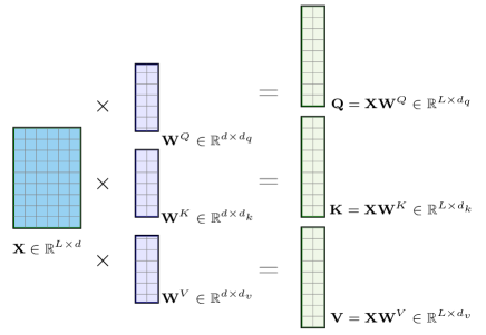
Figure 1: Diagrammatic representation of the computation of the attention matrix $\mathbf{A}$. An input sequence of length $L$ and embedding dimension $d$ is combined with learned weights to produce query, key and value matrices $\mathbf{Q,K}$ and $\mathbf{V}$ respectively.

2.3 The Rise of the Transformer

Seminal work by Vaswani et al. (2017) introduced an architecture dubbed the transformer, which is constructed entirely around self-attention. They showed that state-of-the-art performance in neural machine translation can be achieved without the need for any CNN or RNN components; as they put simply attention is all you need. Such was the impact of this work that there has since been an explosion of transformer variants as researchers strive to develop more efficient implementations and new applications (Tay et al., 2020). It is the original architecture by Vaswani et al. (2017) that inspired the architecture proposed in this article, and as such the remainder of this section focuses on describing the inner workings of this model.

As can be seen in Figure 2, the transformer consists of two sections: an encoder and a decoder. Within each encoder and decoder there exists a transformer-block, which contains the multi-head attention mechanism. In the context of neural machine translation, one could think of this set up as the encoder encoding a sentence in English, transforming the input into a certain representation, and the decoder taking this representation and performing the translation to French. To ensure the model only attends to words it has seen up to a certain point when decoding, an additional causal mask is applied to the input sentence. As an example, this may be the equivalent of only providing inputs $x_{0}^{i}\dots x_{2}^{i}$ of an input sequence of say $L=5$ but requiring the decoder to output predictions up to $y_{L=5}^{t}$.

We focus our discussion on the transformer block without this causal mask since it is this block that is most relevant when we come to classification tasks later in this chapter. Notwithstanding, there is scope for further study to investigate the usefulness of applying a causal mask to the input sequence for early light curve classification. This would present an architecture that does not require full phase light curve information for predictions. By applying a causal mask, one can build a classifier that can ingest partial light curves and still provide predictions. Then by varying the amount of masking (i.e. increasing or decreasing the amount of the light curve that is visible to the network) we can investigate the feasibility of early light curve classification.

2.3.1 Multi-Headed Scaled Dot Product Self-Attention

Whilst the main building block used by Vaswani et al. (2017) is indeed the self-attention mechanism, they modified the typical dot-product attention by introducing a scaled element. This resulted in a new mechanism called the scaled dot-product attention which is similar to Equation 4 but with the input to the softmax scaled down by a factor of the dimensionality of the keys, $d_{k}$. The motivation for introducing a scaling factor is to control possible vanishing gradients that may arise from large dot-products between embeddings. The new formulation for this mechanism can be expressed as

$$\text{Attention}(\mathbf{Q},\mathbf{K},\mathbf{V})=\mathbf{A}=\text{softmax}\left(\frac{\mathbf{Q}{\mathbf{K}}^{\top}}{\sqrt{d_{k}}}\right)\mathbf{V}.$$ (5)

This now scaled version of the self-attention module was extended further to also have multiple heads $h$, which allows for the model to be able to learn from many representation subspaces at different positions simultaneously (Vaswani et al., 2017). Similar to normal self-attention calculations show in Section 2.2, this can be pictorially understood with Figure 3 and by concatenating the attentions for each head:

$$\text{MultiHead}\left(\textbf{Q},\textbf{K},\textbf{V}\right)=\boldsymbol{\mathsf{A}}=\text{Concat}[\mathbf{A}_{1},\dots,\mathbf{A}_{h}]\textbf{W}^{O},$$ (6)

where $\mathbf{A}_{i}=\text{Attention}\left(\textbf{Q}_{i},\textbf{K}_{i},\textbf{V}_{i}\right)$. With each $\mathbf{A}_{i}\in\mathbb{R}^{L\times d_{v}}$, the result of a final linear transformation of all concatenated heads, $\text{Concat}[\mathbf{A}_{i},\dots,\mathbf{A}_{h}]\in\mathbb{R}^{L\times hd_{v}}$ with learned output weights $\mathbf{W}^{O}\in\mathbb{R}^{hd_{v}\times d}$, produces the multi-headed attention matrix $\boldsymbol{\mathsf{A}}\in\mathbb{R}^{L\times d}$.

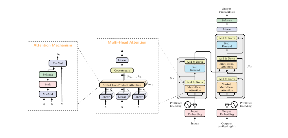
Figure 2: Layout of the original transformer architecture defined in Vaswani et al. (2017). The multi-head attention unit has been zoomed-in to reveal the inner workings and key component of the scaled dot-product attention mechanism. Note the two grey boxes on the left and right of the architecture. These are both transformer blocks, with $N$ indicating how many times each block is stacked upon itself. This diagram is derived from Figure 1 and Figure 2 of Vaswani et al. (2017) and Figure 1 of Tay et al. (2020)

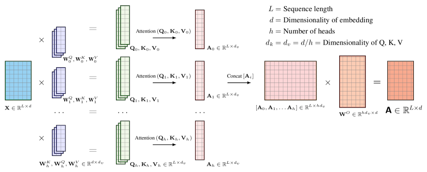
Figure 3: Diagrammatic representation of the computation of the multi-head attention. Instead of computing attention once, the multi-head mechanism divides the input with sequence length $L$ and embedding dimension $d$ by number of heads $h$ to compute the scaled dot-product attention over each subspace simultaneously. These independent attention matrices are then concatenated together and linearly transformed into an attention matrix $\mathbf{A}\in\mathbb{R}^{L\times d}$. The above diagrammatic representation assumes the dimensionality of keys $d_{k}$ is the same as the dimensionality of the values $d_{v}$.

2.3.2 Additional Transformer-Block Components

As can be seen Figure 2 inside the transformer-block, there is also a pathway that skips the multi-head attention unit and feeds directly into an Add & Norm layer. This skip-connection, often referred to a residual connection (He et al., 2016), allows for a flow of information to bypass potentially gradient-diminishing components. The information that flows around the multi-head attention block is combined with the output of the block and then normalised using layer normalisation (Ba et al., 2016) by

$$\mathbf{X}\leftarrow\text{LayerNorm}(\text{MultiHeadSelfAttention}(\mathbf{X}))+\mathbf{X}.$$ (7)

A feed-forward network follows, comprised of two dense layers with the first using ReLU activation (Nair & Hinton, 2010) and the second without any activation function. A similar skip connection occurs, but instead bypasses the feed-forward network, before being combined again and layer-normalised. It should be noted that all operations inside the transformer-block are time-distributed, which is to say that each word or vector representational embedding, is applied independently at all positions. When combining these elements together, this results in a single transformer-block:

$$\mathbf{X}\leftarrow\text{LayerNorm}(\text{MultiHeadSelfAttention}(\mathbf{X}))+\mathbf{X}$$

$$\mathbf{X}\leftarrow\text{LayerNorm}(\text{FeedForward}(\mathbf{X}))+\mathbf{X},$$ (8)

where $$\mathbf{X}$$ is the input embedding to the transformer-block.

2.3.3 Input Embedding and Positional Encoding

The inputs to the transformer are word embeddings created from typical vector representation algorithms such as word2vec. Applying this transformation projects each word token into a vector representation on which computations are made. Additionally, recall that attention is computed on sets of inputs, and thus the computation itself is permutation invariant. While this gives strengths to this model in terms of parallelism, a drawback of this is the loss of temporal information that would usually be retained with RNNs. A consequence of this is the need for positional encodings to be applied to the input embeddings. In Vaswani et al. (2017) the positional encoding $\mathbf{P}\in\mathbb{R}^{L\times d}$, which is used to provide information about a specific position in a sentence, is computed by a combination of sine and cosine evaluations at varying frequencies. Assume $l$ to be a particular position location in an input sequence, with $l=1,\dots,L$, and embedding index $k=1,\dots,d$, then

$$\mathbf{P}_{lk}=\begin{cases}\sin({\omega_{k}}.l),&\text{if}\ k\text{ even}\\ \cos({\omega_{k}}.l),&\text{otherwise}\end{cases}$$ (9)

$$\text{where }\omega_{k}=\frac{1}{10000^{2k/d}}.$$

Provided the dimension of the word embedding is equal to the dimension of the positional encoding, the positional vector $\boldsymbol{\mathrm{p}}_{l}\in\mathbb{R}^{d}$ corresponding to a row of the matrix $\mathbf{P}$ is added to the corresponding word embedding $\boldsymbol{\mathrm{x}}_{l}$ of the input sequence $[\boldsymbol{\mathrm{x}}_{1},...,\boldsymbol{\mathrm{x}}_{n}]$ (Chen et al., 2021):

$$\boldsymbol{\mathrm{x}}_{l}\leftarrow\boldsymbol{\mathrm{x}}_{l}\oplus\boldsymbol{\mathrm{p}}_{l}.$$ (10)

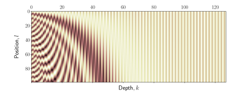
Figure 4: A 128-dimensional positional encoding for a sequence of length of 100. This can be understood as each row representing the encoding vector for that position in the sequence.

For a visual representation of the position encoding see Figure 4, which depicts the positional encoding for a 128-dimensional by 100 sequence length input embedding. Using positional encoding in this way allows for the model to have access to a unique encoding for every position in the input sequence. The motivation for using sine and cosine functions are such that the model is also able to learn relative position information since any offset, $\boldsymbol{\mathrm{p}}_{l+\text{offset}}$ can be represented as a linear function of $\boldsymbol{\mathrm{p}}_{l}$ (Vaswani et al., 2017).

3 The Time-Series Transformer: T2

In this section we present our transformer architecture for time series data, which is based on the self attention mechanism and the transformer-block. Our work is motivated by photometric classification of astronomical transients but generally applicable for classification of general time-series. The time-series transformer architecture that we propose supports the inclusion of additional features, while also offering interpretability. Furthermore, we include layers to support the irregularly sampled multivariate time-series data typical of astronomical transients.

3.1 Architecture

Our architecture, referred to from herein as t2, shown in Figure 5, has several key differences compared to the original transformer shown in Figure 2. The first of these differences is the removal of the decoder. As the task at hand is classification, a single transformer-block is sufficient (Tay et al., 2020). Another difference can be seen with the additional two layers prior to positional encoding unit, which are Gaussian Process Interpolation and Convolutional Embedding. In conjunction with these two layers is a Concatenation layer that is able to add an arbitrary number of additional features to the network. These layers process the astronomical input sequence data and pass it to a typical transformer-block. The output of the transformer-block is then passed through a new Global Average Pooling layer, before finally being passed through a softmax function that provides output probabilities over the classes considered.

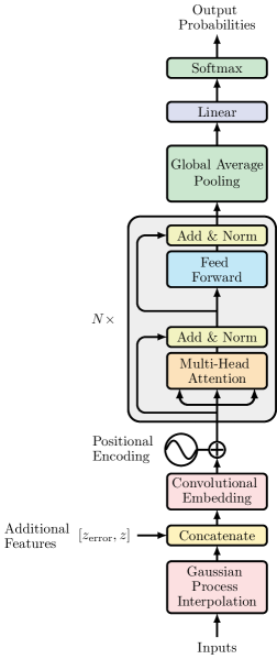
Figure 5: Schematic of the time-series transformer (t2) architecture. Raw time-series data is processed through the Gaussian process interpolation layer, followed by a concatenation layer to include any additional features. A convolutional embedding layer follows to transform the input into a vector representation, with a positional encoding applied to the embedding vector. This is passed as input into the transformer-block, where the multi-head attention block is the same as that shown in Figure 2. The output of which is then passed through a global average pooling layer and finally a linear layer with softmax to output class prediction probabilities for the objects. This diagram is adapted from the Encoder block in Figure 1 of Vaswani et al. (2017).

3.2 Irregularly Sampled Multivariate Time-series Data

With neural machine translation the input consisted of a sequence of words that form a sentence. While this is similar for astronomical transients in the sense that one has a sequence of observations that form a light curve, there are several differences that are important to address. It will be useful to review the kind of data one is dealing with and to make some definitions (adapted from Fawaz et al., 2019) with regards to the task of astronomical transient classification. In general, the data that one observes can be viewed as an irregular multivariate time-series signal:

Definition 3.1.

A univariate time-series signal $\boldsymbol{\mathrm{x}}=[x_{1},x_{2},\dots,x_{T}]$ consists of an ordered set of $T$ real values with $\boldsymbol{\mathrm{x}}\in\mathbb{R}^{T}$.

Definition 3.2.

An $M$-dimensional multivariate time-series signal, $\boldsymbol{\mathrm{X}}=[\boldsymbol{\mathrm{x}}_{1},\boldsymbol{\mathrm{x}}_{2},\dots,\boldsymbol{\mathrm{x}}_{M}]$ consists of $M$ univariate time series with $\boldsymbol{\mathrm{X}}\in\mathbb{R}^{T\times M}$.

Definition 3.3.

An irregular time-series is a ordered sequence of observation time and value pairs $\left(t_{n},x_{n}\right)$ where the space between observation times is not constant.

Definition 3.4.

A dataset $\mathcal{D}=\{(X_{1},Y_{1}),(X_{2},Y_{2}),\dots,(X_{N},Y_{N})\}$ is a collection of pairs $(X_{i},Y_{i})$ where $X_{i}$ could either be a univariate or multivariate time series with $Y_{i}$ as its corresponding one-hot label vector. For a dataset containing $C$ classes, the one-hot label vector $Y_{i}$ is a vector of length $C$ where each element is equal to $1$ for the index corresponding to the class of $X_{i}$ and $0$ otherwise.

The goal for general time-series classification consists of training a classifier on a dataset $\mathcal{D}$ in order to map from the space of possible inputs to a probability distribution over the class variable labels. For photometric classification of astronomical transients, the light that is observed is collected through different filters, also known as passbands, that allow frequencies of light within certain ranges to pass through. Observations collected over a period of time for a particular celestial object form a light-curve. A light-curve is irregularly sampled in time and across passbands which further complicates the task.

3.2.1 Data Interpolation with Gaussian Processes

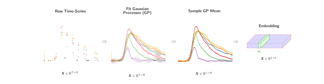
Figure 6: The three-stage process of transforming an astronomical transient light curve from raw photometric time-series data to a vector representation suitable as input to the time-series transformer. First, Gaussian process regression is carried out to regularly sample the light curve. The Gaussian process mean is evaluated at $L$ time points $l$ for each of $M$ passbands, and projected to dimension $d$ via a 1-dimensional convolutional embedding (Lin et al., 2013) at each point $l$ such that final input sequence $\boldsymbol{X}\in\mathbb{R}^{L\times d}$. The resulting embedding matrix is then shown in blue, where for example a $d$-length vector for a single input position highlighted in green.

The raw time-series that is observed is irregularly sampled with heteroskedastic errors. A technique widely used to overcome missing data, and that can also provide uncertainty information is Gaussian process regression (Rasmussen, 2004). This technique is a popular method that has been applied to SNe light curves for many years, e.g Lochner et al. (2016). Gaussian processes represent distributions over functions $f$ that when evaluated at a given point ${x}$ is a random variable $f({x})$, with mean $\mathop{\mathbb{E}[f({x})]}=m({x})$ and covariance between two sampled observations ${x},{x}^{\prime}$ as $\text{Cov}(f({x},{x^{\prime}}))=\mathbf{K}_{f}({x},{x^{\prime}})$, where $\mathbf{K}_{f}(\cdot,\cdot)$ is a kernel.

An important aspect of applying Gaussian process interpolation to data is the choice of kernel. It was discovered in Boone (2019) that for general transients a 2-dimensional kernel that incorporates both wavelength (i.e. passband) information as well as time works well. It can be seen in Boone (2019) that by use of a 2-dimensional kernel, correlations between passbands are leveraged and predictions in passbands that do not have any observations are still possible. Though it should be noted that predictions in passbands without observations will have significantly increased variance and extrapolations errors. As such, we use the Matern kernel (Rasmussen, 2004) that is parametrised by $\nu$ which controls the smoothness of the resulting function and set to $\nu=3/2$. By performing Gaussian process regression and then sampling the resulting Gaussian process at regular intervals, we transform our previously irregular multivariate time-series to a now well sampled regular multivariate signal. The Gaussian process mean is sampled at regular points in time to produce $\mathbf{X}\in\mathbb{R}^{L\times M}$, where $L$ is the sampled time sequence length and $M$ is the number of passbands. This procedure is illustrated in Figure 6 (along with a final convolutional embedding explained in the following Section 3.3).

3.3 Convolutional Embedding

With neural machine translation applications the inputs to the original transformer architecture take in word embeddings that had been derived from a typical vector representation algorithm such as word2vec. In a similar manner, embeddings for the now interpolated time-series data are required. We adopt a simple 1-dimensional convolutional embedding, with kernel size of 1 and apply a ReLU non-linearity. Inspired by Lin et al. (2013), a 1-dimensional convolution allows for a transformation from $k$-dimensional space to a $k^{\prime}$-dimensional space whilst operating over a single time window of size of 1. For our purposes, using this convolution allows for dimensionality to be scaled from $M$ to $d$ dimensions without affecting the spatio-temporal input. Therefore, this operation transforms the original input of $M$-dimensional time-series data points, i.e. time-series data points across $M$ passbands, into a $d$-dimensional vector representation ready for input into the transformer-block. This operation is akin to a time-distributed, position-wise feed-forward neural network operating on each input position.

3.4 Global Average Pooling

We also introduce a layer that performs global average pooling (GAP) on the output of the transformer-block. The motivation for adding a GAP layer following the transformer-block was inspired by work in Zhou et al. (2015). The GAP layer, originally proposed by Lin et al. (2013), has become a staple in modern CNN architectures due to its usefulness in interpretable machine learning. In previous works on 2-dimensional images, GAP layers are used as a replacement to common fully connected layers to avoid overfitting since there are no parameters to optimise. Another useful advantage over the fully connected layer is the averaging in a GAP layer averages out the spatial information leaving it more robust to translations of the inputs (Lin et al., 2013). Similar to 2-dimensional inputs, using a GAP layer on the 1-dimensional time-series, proves robustness to translations in the input.

By adapting the description found in Zhou et al. (2015), one can apply a GAP layer to a time-series. Let $f_{k}(l)$ represent the activation of a particular embedded dimension $k$ at a location $l$, where $k=1,\dots,d$ and $l=1,\dots,L$. Then a GAP layer can be computed by taking the average over time for each feature map $F_{k}=\sum_{l}f_{k}(l)$.

3.5 Class Activation Maps (CAM)

A nice feature of using a GAP layer is that one can determine the influence of $f_{k}(l)$ on predictions for a given class $c\in C$ by considering the associated score $S_{c}$ that is passed into the softmax layer (Zhou et al., 2015). This is calculated from the final fully connected weights $w^{c}_{k}$ and the feature maps $F_{k}$ as $S_{c}=\sum_{k}w^{c}_{k}\cdot F_{k}=\sum_{l}\sum_{k}w^{c}_{k}\cdot f_{k}(l)$.

The class activation map (CAM) for a given class $c$ is then given by

$$M_{c}(l)=\sum_{k}w^{c}_{k}f_{k}(l).$$ (11)

Since $S_{c}=\sum_{l}M_{c}(l)$, it is possible to use $M_{c}(l)$ to directly gauge the importance of the activation at input location $l$ in leading to the classification of class $c$.

3.6 Inputting Additional Information

The time-series transform, t2, is designed to be malleable such that one can add further features if desired. For the purposes of the current study of photometric classification, only redshift information has been added. In many photometric classifiers, photometric redshift $z$, has consistently been a feature of high importance (e.g. Boone, 2019). As one particular example of the type of additional features that can be added, photometric redshift $z$ and the associated error $z_{\text{error}}$ are included.

Additional features could in principle be incorporated in the time-series transformer in a variety of different manners. To leverage the power of neural networks to model complex non-linear mappings, such additional features should feed through non-linear components of the architecture. On the other hand, recall from Section 3.5 that in order to compute a CAM (class activation map), the output of the GAP layer must pass directly into the linear softmax layer. Hence, incorporating additional features at this stage of the architecture will not be effective unless a non-linear activation is introduced, which would destroy the interpretability of the model.

To preserve our ability to compute CAMs, there are several other possible locations in the architecture where one could consider including additional features. The most natural point is immediately prior to the convolutional embedding layer (see Figure 5). Adding features at this location allows for all information to be passed throughout the entire network. Nevertheless, there are alternative ways in which additional features can be incorporated at this point.

The most obvious way to incorporate additional features is to essentially consider them as a additional channels and concatenate in the dimension of the $M$ passbands to redefine the input as $\boldsymbol{\mathrm{X}}\in\mathbb{R}^{L\times M}\rightarrow\boldsymbol{\mathrm{X}}\in\mathbb{R}^{L\times M^{\prime}}$, where $M^{\prime}=M+R$, and $R$ is the number of features to add. This essentially broadcasts the additional information to each input position in $l$.

The alternative is to concatenate in the dimension of the $L$ time sequence samples, which transforms the input as $\boldsymbol{\mathrm{X}}\in\mathbb{R}^{L\times M}\rightarrow\boldsymbol{\mathrm{X}}\in\mathbb{R}^{L^{\prime}\times M}$, where $L^{\prime}=L+R$. There are several advantages for choosing the approach of concatenating to $L$ rather than $M$. Firstly, this approach allows one to pay attention to the additional features explicitly. Secondly, it gives activation weights for the additional features, which in our case is redshift and redshift error, so the impact of the additional features can be interpreted. So, while in principle one could consider concatenating to either $L$ or $M$, we advocate concatenating to $L$.

3.7 Trainable Parameters and Hyperparameters

The time-series transformer, t2, model contains a set of trainable parameters that stem from the weights contained in the transformer-block as well as learned weights at the embedding layer and final fully connected layer. The first layer with trainable parameters is the convolutional embedding layer. The numbers of parameters for a general convolutional layer is given by

$$[M\times w\times d]+d,$$

where $M$ denotes the number of input channels or passbands, $w$ refers to the kernel window size, which in this case is 1, and $d$ is the dimensionality of the embedding. Continuing through the model, the number of trainable parameters for the multi-head attention unit has 4 linear connections, including $\mathbf{Q}$, $\mathbf{K}$, $\mathbf{V}$ and one after the concatenation layer, i.e. $\boldsymbol{\mathrm{W}}^{Q}$, $\boldsymbol{\mathrm{W}}^{K}$, $\boldsymbol{\mathrm{W}}^{V}$ and $\boldsymbol{\mathrm{W}}^{O}$. Recall that for multi-head attention we set $hd_{v}=d$ (see Figure 3), hence the number of parameters for $\boldsymbol{\mathrm{W}}^{Q}$, $\boldsymbol{\mathrm{W}}^{K}$, $\boldsymbol{\mathrm{W}}^{V}$ and $\boldsymbol{\mathrm{W}}^{O}$ across all of the $h$ heads is identical. The number of layer normalisation parameters is simply the sum of weights and biases together with the feed forward neural network weights of the input multiplied by the weights of the output plus the output biases (Zhang et al., 2021). Combining all units inside the transformer block together yield

$$N\times{\underbrace{\big{(}4\times\left[(d\times d)+d\right]\big{)}}_{\text{Multi-Head Attention}}}+{\underbrace{\big{(}2\times 2d\big{)}}_{\mathclap{\text{Layer Norm}}}}+{\underbrace{\big{(}d\times d_{\text{ff}}+d_{\text{ff}}\big{)}+\big{(}d_{\text{ff}}\times d+d\big{)}}_{\text{Feed Forward}}}$$

where $N$ refers to how many times one stacks the transformer-block upon itself, and $d_{\text{ff}}$ refers to the number of neurons in the feed forward network inside the transformer-block. Since there are no trainable parameters with the GAP layer, the final fully connected linear layer with softmax results in a remaining number of trainable parameters of

$$\left([d\times C]+C\right),$$

where $C$ refers to the number of classes.

Of the parameters discussed above, there are some that are fixed due to the problem at hand, such as $M$ number of passbands and $C$ classes to classify. But there are also other parameters that are not necessarily trainable that are considered hyperparameters. These include: the dimensionality of the input embedding $d$, the dimensionality of the feed forward network inside the transformer-block $d_{\text{ff}}$, the number of heads to use in conjunction with the multi-head attention unit $h$, the percentage of neurons to drop when in training using the dropout method (Srivastava et al., 2014) droprate, the number of transformer-blocks $N$, and the learning rate learning_rate (discussed further in Section 4.4).

4 Implementation, Evaluation Metrics & Training

We leverage modern machine learning frameworks to develop the time-series transformer implementation, t2, in a modular manner for ease of use and future extension. We present the key evaluation metrics that we use to measure the performance of the classifier and the motivation for particular types of metrics in relation to the photometric astronomical transient classification problem that we consider in Section 5. We also discuss the loss function used for training and how hyperparameters are optimised.

4.1 Implementation

We use the machine learning framework of TensorFlow (Abadi et al., 2015) with the tf.keras API for the implementation of our t2 architecture. Our code is available under Apache 2.0 licence and open-sourced. Key data processing software of pandas (Wes McKinney, 2010) and numpy (Harris et al., 2020) has been used heavily for manipulation of input data, with george (Ambikasaran et al., 2015) used for fitting the Gaussian processes. Training of our model has been carried out on a NVIDIA Tesla V100 GPU, where the time taken for a single epoch is 7.8 minutes. With a convergence rate on the order of 130 epochs, a new model can be therefore be trained in approximately 17hrs using the full PLAsTiCC dataset described in the upcoming Section 5.1. On the other hand, inference takes place using CPUs, where for a single light curve if of the order of 1.5 seconds. It should be noted that there is typically an additional 4 seconds overhead for loading the model into memory from disk. However, as inference is to be done for a batch of light-curves at a time in brokering systems, we do not consider this as part of the latency for a single light curve for this discussion. Yet, work by Allam Jr et al. (2023) showed that for deploying models into brokering systems, one can use deep model compression techniques to significantly reduce the overhead for loading a model into memory when batch processing alerts along with improved inference latency as well.

4.2 Performance Metrics

Choice of evaluation metrics is of high importance when considering the performance of a classifier. This is compounded when dealing with imbalanced datasets since most metrics consider the setting of an even distribution of samples among the classes. One must be careful when considering which metrics to evaluate a model’s performance since relatively robust procedures can be unreliable and misleading when dealing with imbalanced data (Branco et al., 2015; Malz et al., 2019).

Typically, threshold metrics are used which consider the rate or fraction of correct or incorrect predictions. Threshold metrics are formulated by combinations of the four possible outcomes a classifier could have with regards to predicting the correct class:

• True Positive (TP): prediction of a given class and indeed it being that class.

• False Positive (FP): prediction of a given class but it does not belong to that class.

• True Negative (TN): prediction that an object is not a particular class and it is indeed not that class.

• False Negative (FN): prediction that an object is not a particular class but it is in fact that class.

From these outcomes common threshold metrics can be formulated, with perhaps the most common threshold metric being accuracy, which is the number of correctly classified samples over the total number of predictions. However, for imbalanced data results on accuracy alone can be misleading as a model can achieve high accuracy by simply classifying the majority class. More robust metrics for imbalanced data are precision and recall since their focus is on a particular class:

$$\mathrm{Precision}=\frac{\mathrm{TP}}{\mathrm{TP+FP}},\quad\mathrm{Recall}=\frac{\mathrm{TP}}{\mathrm{TP+FN}}.$$ (12)

Precision gives the fraction of samples predicted as a particular class that indeed belong to the particular class. While recall, also known as the true positive rate, indicates how well a particular class was predicted.

4.2.1 Confusion Matrix

One way to visually inspect the performance of a classifier with regards to threshold metrics is by the confusion matrix. The confusion matrix provides more insight into the performance of the model and reveals which classes are being predicted correctly or incorrectly. Often these tables are normalised across the rows to give probabilities in order to provide a more intuitive understanding. A perfect classifier across all classes would therefore be equivalent to the identity matrix with all ones along the diagonal and zero elsewhere.

4.2.2 Receiver Operating Characteristic

An important point to note is that threshold metrics alone assume the class imbalance present in the training set is of the same distribution as that of the test set (He & Ma, 2013). On the other hand, a set of metrics built from the same fundamental components as threshold metrics, called rank metrics, do not make any assumptions about class distributions and therefore are a useful tool for evaluating classifiers based on how effective they are at distinguishing between classes (Gupta et al., 2020).

Rank metrics require that a classifier predicts a probability of belonging to a certain class. From this, different thresholds can be applied to test the effectiveness of classifiers. Those models that maintain a strong probability of being a certain class across a range of thresholds will have good class separation and thus will be ranked higher.

The most common of this type of metric is the receiver-operating-characteristic (ROC) curve (Fawcett, 2006), which plots the true positive rate verses the false positive rate to estimate the behaviour of the model under different thresholds. The ROC curve is then used as a diagnostic tool to evaluate the model’s performance, with every point on graph representing a given threshold. Interpolating between these points forms a curve, with the area under the curve (AUC) quantifying performance. A classifier is effectively random if the AUC is 0.5 and, conversely, is a perfect classifier if the AUC is equal to 1.0. It is common when reporting the AUC for multi-class classification to give the macro- and micro-averaged score. A macro-averaged score is calculated by considering the metric independently for each class and then taking an average. In this way, all classes are treated equally which is troublesome if one has highly imbalanced data. A micro-averaged score on the other hand aggregates the contributions of all classes in order to calculate the metric. Therefore, it is advisable to consider micro-average scores when dealing with imbalanced datasets.

4.2.3 Precision-Recall Trade-Off

An alternative diagnostic plot to the ROC curve is the precision-recall (PR) trade-off curve. This is used in a similar way to the ROC curve but instead focuses on the performance of the classifier to the minority class, and hence is more useful for imbalanced classification problems (Brownlee, 2020). Much like the ROC curve, points on the curve represent different classification thresholds with a random classifier resulting in an AUC equal to $0.5$ and a perfect classifier resulting in an AUC of 1.0. In addition, macro- and micro averaged scores can also be computed for PR curves, and the preference for using micro-averaged scores in the imbalanced setting remains.

4.3 Multi-Class Logarithmic-Loss

The underlying algorithm that governs the usefulness of neural networks is the stochastic gradient decent (SGD) optimisation algorithm that updates the weights of the network according to the backpropagation algorithm (Rumelhart et al., 1986). While performance metrics give an indicator as to how well a model is able to distinguish between classes, to be able to train and improve the model one must have a differentiable loss function. Extensive investigations by Malz et al. (2019) showed that the most suitable differentiable loss-function for the problem of transients classification is a probabilistic loss function. Probabilistic loss functions are used in cases where the uncertainty of a prediction is useful and the problem at hand is best served with quantification of the errors rather than a binary answer of correct or incorrect. The probabilistic loss function they suggest is the multi-class weighted logarithmic-loss that up-weights rarer classes and defines a perfect classifier as one that achieves a score of zero, and is given by

$$\boldsymbol{\mathcal{L}}=-\left(\frac{\sum_{i=1}^{C}w_{i}\sum_{j=1}^{N_{i}}\frac{y_{ij}}{N_{i}}\ln p_{ij}}{\sum_{i=1}^{C}w_{i}}\right),$$ (13)

where $C$ refers to the number of classes in the dataset and $N_{i}$ the number of objects in the $i$-th class. The predicted probability of an observation $i$ belonging to class $j$ is given by $p_{ij}$. For our investigation we opt for a flat-weighted multi-class logarithmic-loss as described in Boone (2019) that assigns all classes in the training set the same weight of $w_{i}=1$. To consider the original metric put forth in Malz et al. (2019) and use the weighting scheme designed for the PLAsTiCC competition, one would also need to include the additional anomaly classes (class 99) that existed in the PLAsTiCC test set. By ignoring class 99 one can better compare later analyses between the original PLAsTiCC training set and our modified dataset (described in upcoming Section 5.1).

4.4 Training

In order to train a model with the t2 architecture, we need to establish the choice of optimisation algorithm and associated parameters that will be used to update the weights of the network. We use a variant of the SGD optimisation algorithm mentioned in Section 4.3 called ADAM (Kingma & Ba, 2014). An important aspect to consider when training a model using any optimisation algorithm is the learning schedule and corresponding learning rate. The initialisation value of the learning rate can be seen as a hyperparameter to be optimised for separately with hyperparameter optimisation (discussed in the next section). It is typically beneficial to introduce a learning schedule to reduce the learning rate as training progresses (Goodfellow et al., 2016). We indeed adopt a learning schedule, reducing the learning rate by 10% if it is observed that our loss value does not decrease within 5 epochs. To ensure the model does not overfit, we monitor the ratio of validation loss with the training set loss.

4.5 Hyperparameter Optimisation

As discussed in Section 3.7, t2 contains a set of fixed parameters such as $M$ and $C$, and a set of tunable hyperparameters. Choosing the best set of hyperparameters can be framed as an optimisation problem expressed as

$$\theta^{*}=\operatorname*{arg\,min}_{\theta\in\Theta}g(\theta),$$ (14)

where $g(\theta)$ is an objective score to be minimised and evaluated on a validation set, with the set of hyperparameters $\theta$ being able to take any value defined in the domain of $\Theta$. The objective score for our purposes is the logarithmic-loss defined in Equation 13 and the set of hyperparameters that yield the lowest objective score is $\theta^{*}$. The goal is to find the model hyperparameters that yield the best score on the validation set metric (Frazier, 2018).

Traditionally hyperparameter optimisation has been performed with either random search or a grid search over the set of parameters in $\Theta$, which can be time consuming and inefficient. Instead a Bayesian optimisation approach is used that attempts to form a probabilistic model mapping hyperparameters to a probability distribution for a given score.

To choose the best performing hyperparameters we use the Tree-structured Parzen Estimator (TPE) algorithm (Bergstra et al., 2011) that is implemented in the optuna package (Akiba et al., 2019) with 5 fold cross-validation. For this we impose a Gaussian prior with weight equal to 1, and use 24 candidate samples.

5 Results

We apply our time-series transformer architecture to the problem of photometric classification of astronomical transients. As noted in Section 1 typical astronomical data that are available for training a photometric classifier are highly imbalanced, with a large number of spectroscopically confirmed SNIa compared to other classes, and non-representative, since observations are biased towards lower redshift objects. Consequently, the training data are non-representative of the test data. For robust and accurate classification, training datasets should be representative of the test data. Works by Boone (2019) and Revsbech et al. (2018) present techniques that help address this problem of non-representativity, transforming the training data to be more representative of the true test data through data augmentation. This process is involved and can be decoupled from the design of architecture of the classifier. Therefore in this current article, as a first step we consider training data that is representative in redshift but imbalanced. In future work we will consider the combination of t2 with augmentation techniques described above or other recent methods such as those described in Burhanudin et al. (2021) that use focal loss function with a recurrent neural network to address the representativity problem.

5.1 Astronomical Transients Dataset

To be able to evaluate our architecture in a representative setting, but also to test the models resilience to class imbalance, we utilise the PLAsTiCC dataset (The PLAsTiCC team et al., 2018). The complete dataset contains synthetic light curves of approximately 3.5 million transient objects from a variety of classes simulated to be observed in 6 passbands using a cadence defined in Kessler et al. (2019).

The majority of events that exist in the dataset were simulated to be observed with the Wide-Fast-Deep (WFD) mode, which compared to the Deep-Drilling-Fields (DDF) observing mode, is more sparsely sampled in time and has larger errors. Originally crafted for a machine learning competition, the entire PLAsTiCC dataset was divided into two parts, with $<1\%$ initially being given to participants in the competition that was highly non-representative of the other part. Following the close of the competition all data are now publicly available. For our purposes, we use the complement to what was initially released and construct a new training and test set from the remaining $99\%$ of the data (without anomaly class 99). By doing so, the dataset is now representative in terms of redshift, but remains highly imbalanced in terms of the classes. The number of samples per class used to evaluate our architecture can be found in Table 1.

Table 1: Number of samples of the PLAsTiCC data used for evaluation of the t2 model. Note the largely imbalanced dataset distribution of Supernovae Type-Ia (SNIa) objects compared to other classes.

Class	Number of Samples (%)
$\mu-\text{Lens-Single}$	1,303 (0.037%)
TDE	13,552 (0.389%)
EB	96,560 (2.775%)
SNII	1,000,033 (28.741%)
SNIax	63,660 (1.830%)
Mira	1,453 (0.042%)
SNIbc	175,083 (5.032%)
KN	132 (0.004%)
M-dwarf	93,480 (2.686%)
SNIa-91bg	40,192 (1.155%)
AGN	101,412 (2.915%)
SNIa	1,659,684 (47.700%)
RRL	197,131 (5.666%)
SLSN-I	35,780 (1.028%)
Total	3,479,456 (100%)

5.2 Classification Performance

Of the model parameters in the time-series transformer, t2, there are a subset of hyperparameters that are tunable and can be optimised for (see Section 4.5). Through application of the TPE Bayesian optimisation method on a validation set constructed from $10\%$ of the training set, using 5-fold cross-validation we obtained the parameters which gave the lowest objective score. The results of which can be found in Table 2.

Table 2: The time-series transformer, t2, contains 6 hyperparameters to be optimised. The set of parameters and learning rate that scored the lowest objective score using 5-fold cross-validation and the TPE Bayesian optimisation method is shown here, along with the search space considered. All parameters have been chosen from the set of options listed in the Search Space column below, with the exception of the learning_rate which has been selected from the continuous range within the two values given. To be concise we only show learning_rate to 3 decimal places and advise the reader to refer to the code for full details.

Parameter	Value	Search Space
$d$	32	{32, 64, 128, 512}
$h$	16	{4, 8, 16}
$d_{\text{ff}}$	128	{32, 64, 128, 512}
$N$	1	{1, 2, 4, 8}
droprate	0.1	{0.1, 0.2, 0.4}
learning_rate	0.017	[0.01, 0.1]

When we build our time-series transformer with the hyperparameters shown in Table 2, and train a model using the training data set described in 5.1 we are able to achieve a logarithmic-loss of $0.507$. The confusion matrix depicted in Figure 7 shows good performance across all classes. Both receiver operating characteristic (ROC) and precision-recall (PR) plots, Figure 8 and Figure 9 respectively, show reasonable multi-class classification accuracy, with the exception being towards the Kilonovae and SNIax classes. We suspect this is purely down to the scarcity of sample for Kilonovae and light curve similarity to SNIa around the peak in the case of SNIax (Jha, 2017). Moreover, core-collapse SNe (SNIbc and SNII) can be seen to be also problematic yet we achieve a SNIa purity of 0.94 with a core-collapse SNe cross contamination of $\sim 4.81\%$. This compares to the reported by DES (Vincenzi et al., 2021) and Pan-STARRS (Jones et al., 2018) of acceptable range for cross-contamination of $\sim 8\%$ and $\sim 5\%$ respectively, allowing for our results to useable for cosmological analyses of dark energy equation of state. The performance of our model expectedly degrades when auxiliary information of redshift and redshift error is not included. However, we find it promising that our model with raw time-series information only can still achieve a logarithmic-loss of $0.873$.

It is expected that if a full hyperparameter search can be performed on the full training set by leveraging greater computational resources, it is likely better parameters could be discovered leading to improved performance. While a direct comparison with other methods presented in Hložek et al. (2020) cannot be made since they have been trained with non-representative datasets, the time-series transformer is able to achieve excellent classification performance with minimal feature selection and few trainable parameters by deep learning standards.

It is often the case with machine learning models that, as remarked upon in Hložek et al. (2020) and Lochner et al. (2016), in order to overcome a classification bias towards particular classes, an equal distribution of samples among the classes is often necessary for accurate classification. However, the t2 architecture is able to handle class imbalance very well, and as such our model did not require any data augmentation in order to achieve a good score, unlike other methods. It is uncertain at this time whether this is an inherent property of transformers or the attention mechanism, or perhaps the architecture is simply able to find sufficient discriminative features with far fewer training samples than was previously thought is required for deep learning approaches such as CNNs and RNNs. However, we suspect this will likely be due to the low number of parameters relative to the number of data samples our model has compared to models such as CNNs and RNNs that have far greater number of model parameters that need to be tuned to avoid overfitting and achieve good predictive generalisation. As discussed already, we are yet to consider the case of data that is not representative in redshift, where augmentation techniques will certainly be necessary, which will be the focus of future work.

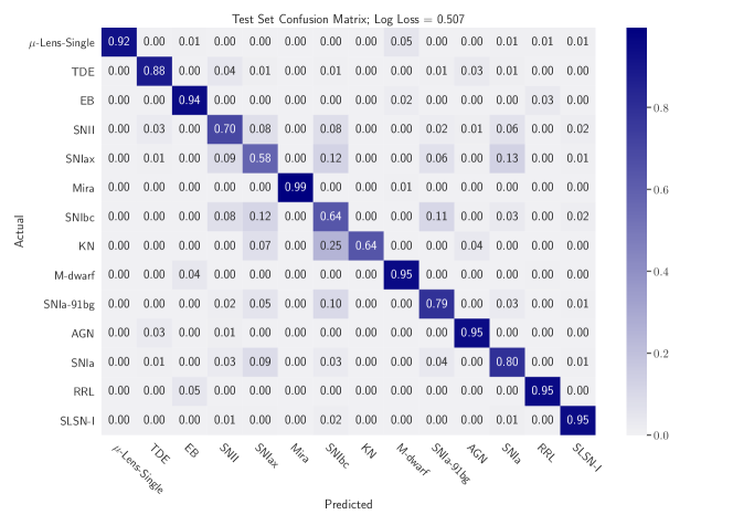
Figure 7: Confusion matrix resulting from application of the time-series transformer, t2, to the PLAsTiCC dataset in a representative setting with imbalanced classes, achieving a logarithmic-loss of 0.507.

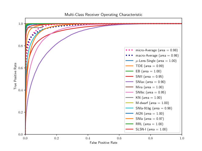
Figure 8: Receiver operating characteristic (ROC) curve, under the same setting as those described in Figure 7. Micro- and macro-averaged AUC scores of 0.98 are achieved across the classes.

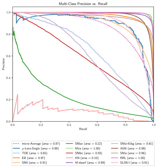
Figure 9: Precision-recall trade-off curve, under the same setting as those described in Figure 7. A micro-averaged AUC score of 0.87 is achieved across the classes. The model understandably struggles with precision for Kilonovae (KN), which only constitutes 0.004% of the training sample.

5.3 Interpretable Machine Learning

Work by Zhou et al. (2015) lead the way forward with major improvements for model interpretability. Their use of the GAP (global average pooling) layer for the localisation of feature importance helped researchers discover methods of visually inspecting a classifier’s performance. In a similar regard, a GAP layer is included in the t2 architecture to allow for model interpretability through the visualisation of the various feature maps as a function of sequence length. As discussed in Section 3.5, one can compute a CAM (class activation map) which can help determine how the features at each input position have influenced the final prediction. Also recall from Section 3.6 that t2 allows for concatenation of arbitrary additional features; in this work we consider the addition of redshift information.

Of the two options for concatenation, either in time or passband, we adopt the approach of concatenating to $L$ in time to give $L^{\prime}=L+R$, where $R=2$ with redshift and redshift error added as additional features. This has the advantage that we explicitly pay attention to redshift information and also get interpretability with respect to redshift information (see Section 3.6). For completeness, we also re-run the photometric classification analysis discussed previously by concatenation to $M$, but we do not observe as good a performance as concatenating to $L$. As we suspected, this may well be because we are explicitly paying attention to redshift in the multi-head attention mechanism, whereas by concatenating to $M$ we do not get this benefit.

The CAM can then be computed by Equation 11, where $M_{c}(l^{\prime})$ indicates the influence each position of the input sequence has on classification, which also includes redshift information, i.e. $l^{\prime}=1\ldots,L+R$. We apply a min-max scaling and normalise the CAM such that $\sum_{1}^{L+R}M_{c}(l^{\prime})=1$, so that the relative activation weights can be interpreted as a percentage.

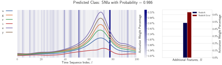
(a) Class activation map for a SNIa drawn from the test set.

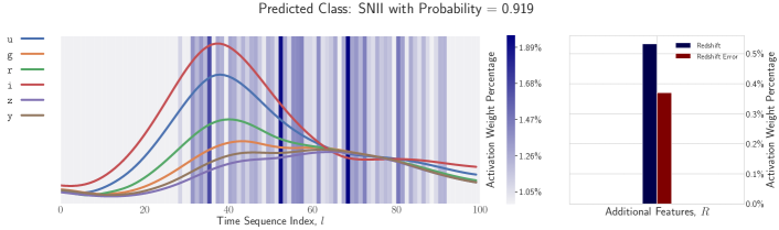
(b) Class activation map for a SNII drawn from the test set.

Figure 10: Class activation maps (CAM) for two types of Supernova drawn from the test set, with lightcurves for bands $ugrizy$ over-plotted. For visualisation purposes, a min-max scaling is applied to the class activations as well as a normalisation to each CAM such that $\sum_{l^{\prime}}M_{c}(l^{\prime})=1$, such that the relative activation weights can be interpreted as a percentage. The left hand side depicts the percentage of activation weight attributed to each position in the sequence, while on the right hand side we show the percentage activation weights associated with any additional features that have been added; in our case redshift and redshift error. The influence of redshift and information can be seen on the right hand side, with $\sim 0.6\%$ and $\sim 1.4\%$ of the total activation weight being attributed these additional features for each object, respectively.

We show in Figure 10 illustrative CAMs for two Supernova classes, over-plotted with the lightcurves themselves. In each panel CAM probabilities for each light curve time point are shown, in addition to the CAM probabilities for the additional features of redshift and redshift error. Notice that for both examples the activation weight is generally low before the initial rise of the light curve. For SNII we see a strong set of weights around the peak with moderate weights observed in the tail, presumably to detect any secondary peak. On the other hand, SNIa has its strongest weights just before and after the peak, possibly capturing information of the width of the profile.

As our architecture is able to include additional features, these can also be inspected and visualised to gain further understanding as to how much importance the model is paying towards them. In our case, with the addition of redshift and redshift error information, we also include bar plots in Figure 10 that depict the activation weight for redshift and redshift error. We inspect the distribution of the activation weights for redshift and redshift error for all classes combined, which can be seen in Figure 11. The majority of activation weighting relating to redshift and redshift error falls around $1\%$. We also explored this distribution on an individual class by class basis but did not find a significant difference across classes. Therefore, there does not seem to be a particular class that benefits from redshift information over another. The distributions indicate that for most objects redshift informations accounts for a relative small proportion of the total activation weights, with a mean of $\sim 1.92\%$. However, it should be noted that this is related to the $L=100$ regularly sampled points on the light curve, many of which are highly informative. Furthermore, we recall that redshift on the whole is indeed important for accurate classification where we achieve a logarithmic-loss of 0.507 when including redshift information and 0.873 when it is not included (Section 5.2).

While we have shown CAMs to be useful for a first attempt to bring interpretability to light curve classification, we acknowledge more recent saliency mapping techniques that address some of the shortcomings of CAMs. We commented earlier that in order to compute CAMs we require the GAP layer. Although we have provided separate motivation for using a GAP layer (see Section 3.4) it may be the case that in the pursuit of better interpretability, requiring a GAP layer unnecessarily restricts the flexibility of our model for possible model extensions. Therefore it would be preferable to have an explainable methodology that does not impose certain characteristics on the architecture itself, and that can ideally probe a model in a black-box fashion. Follow-up work by Selvaraju et al. (2017) presented Grad-CAM that did away with the need for a GAP layer to feed directly into the softmax and was agnostic to the downstream task, but still required access to the internals of the model with gradients. An interpretability method proposed by Petsiuk et al. (2018) introduced randomised input sampling for explanation of black-box models (RISE) to better estimate how salient aspects of the input are for a model’s prediction, without the need for access to model internals nor re-implementation of existing models.

It is expected that future studies for interpretability of photometric classification architectures use techniques similar to RISE that can treat the model as a black-box and yet provide more refined saliency maps.

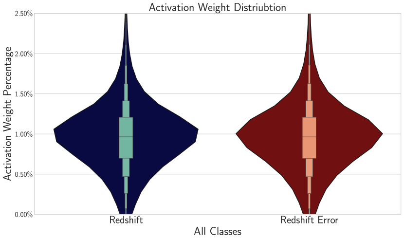
Figure 11: Distribution of activation weights for redshift and redshift error for all classes combined. This plot is constructed for all classes combined (minimal variability was observed across classes when plotted separately). The mean redshift and redshift error activation weights are both $0.96$. In the centre of the plotted distribution we plot letter-value plots (Hofmann et al., 2011) that are better suited to large datasets such as this. The middle box contains 50% of the data, with the median indicated by a line at the midpoint. The next smaller boxes combined contain 25% of the data, with each successive level outward continuing in this fashion containing half of the remaining data.

6 Conclusions

We have constructed a new deep learning architecture designed for photometic classification of astronomical transients that we call the time-series transformer or t2. The architecture is designed in such a way to pay attention not only to light curves but also to any additional features considered (e.g. redshift information) and to also provide interpretability, again not only to light curves but also to additional features. While we are motivated by the problem of astronomical transient classification, the architecture is suitable for general multivariate time-series data.

The time-series transformer, t2, is able to achieve results comparable to the state-of-the-art in photometric classification and does so on extremely imbalanced datasets. Our architecture is able to achieve a logarithmic-loss of 0.507 on the PLAsTiCC dataset defined in Section 5.1 and Table 1. A direct comparison to other latest methods laid out in Hložek et al. (2020) and Gabruseva et al. (2020) is understandably not possible since each classifier has been evaluated on different data under different conditions, nonetheless, t2 is able to achieve the lowest logarithmic-loss on such imbalanced data, without the need for augmentation. Having such an imbalanced dataset, one would expect that there would be bias towards the most common classes, but t2 is robust enough to handle this. As noted in Lochner et al. (2016), accurate photometric classification requires a representative training dataset, but as discussed in Section 1 the data that will be observed with upcoming surveys will be non-representative of the training datasets that are currently available. While this work focuses on the representative setting, the architecture lends itself well to be able to be used in conjunction with latest augmentation techniques, particularly Boone (2019) and Alves et al. (2022) with use of Gaussian processes, that should help to alleviate non-representative training dataset issues, and as such this will be considered in detail in future work.

While t2 is already able to compete with state-of-the-art methods, improvements could be made in future work to modify the components of the architecture, while keeping the broad structure, e.g. by replacing self-attention layers with alternative mixing transforms such as Fourier transforms, which in recent work by Lee-Thorp et al. (2021) have been shown to greatly improve efficiency and yet achieve comparable or, in certain scenarios, superior performance.

The relatively few parameters involved, and hence faster training times, compared to other deep learning methods makes t2 an attractive architecture for potentially combining with active learning methods or even off-line retraining should new data become available. With the small model size, t2 should also appeal to upcoming brokering systems such as FINK (Möller et al., 2021), ANTARES (Matheson et al., 2021) etc. that benefit from low latency and fast inference times when put into production. As we touched on in Section 2.3, the current architecture forgoes the additional decoder found in the original transformer architecture (Vaswani et al., 2017) that applies a casual mask to the input. However, the inclusion of such a mask would provide a natural mechanism within the time-series transformer architecture for early light curve classification, which provides another avenue of future work.

The time-series transformer, t2, minimises the reliance of expert feature selection. Moving away from feature engineering allows the model the freedom to discover patterns that are missed by humans but yet provide powerful discriminative information for classification. The architecture, by virtue of CAMs (class activation maps), offers up a helpful tool for interpretability by inspecting the importance of both light curves and any additional features that are included. It is hoped that with the introduction of the attention mechanism to the field of astronomical photometric classification, further studies will build on this work to improve our ability to attend to the night sky.

Data Availability

All data referenced here can be found freely available online. For the original PLAsTiCC dataset, the reader is advised to explore details laid out in The PLAsTiCC team et al. (2018) and Team & Modelers (2019).

References

- Abadi et al. (2015) Abadi M., et al., 2015, TensorFlow: Large-Scale Machine Learning on Heterogeneous Systems, https://www.tensorflow.org/
- Akiba et al. (2019) Akiba T., Sano S., Yanase T., Ohta T., Koyama M., 2019, in Proceedings of the 25th ACM SIGKDD international conference on knowledge discovery & data mining. pp 2623–2631
- Allam Jr et al. (2023) Allam Jr T., Peloton J., McEwen J. D., 2023, arXiv preprint arXiv:2303.08951
- Alves et al. (2022) Alves C. S., Peiris H. V., Lochner M., McEwen J. D., Allam T., Biswas R., Collaboration L. D. E. S., et al., 2022, The Astrophysical Journal Supplement Series, 258, 23
- Ambikasaran et al. (2015) Ambikasaran S., Foreman-Mackey D., Greengard L., Hogg D. W., O’Neil M., 2015, IEEE transactions on pattern analysis and machine intelligence, 38, 252
- Ba et al. (2016) Ba J. L., Kiros J. R., Hinton G. E., 2016, arXiv preprint arXiv:1607.06450
- Bahdanau et al. (2014) Bahdanau D., Cho K., Bengio Y., 2014, arXiv preprint arXiv:1409.0473
- Bergstra et al. (2011) Bergstra J., Bardenet R., Bengio Y., Kégl B., 2011, in 25th annual conference on neural information processing systems (NIPS 2011).
- Boone (2019) Boone K., 2019, The Astronomical Journal, 158, 257
- Branco et al. (2015) Branco P., Torgo L., Ribeiro R., 2015, arXiv preprint arXiv:1505.01658
- Brauwers & Frasincar (2021) Brauwers G., Frasincar F., 2021, IEEE Transactions on Knowledge and Data Engineering
- Brownlee (2020) Brownlee J., 2020, Tour of Evaluation Metrics for Imbalanced Classification, https://bit.ly/3sxqx9Y
- Brunel et al. (2019) Brunel A., Pasquet J., PASQUET J., Rodriguez N., Comby F., Fouchez D., Chaumont M., 2019, Electronic imaging, 2019, 90
- Burhanudin et al. (2021) Burhanudin U., et al., 2021, Monthly Notices of the Royal Astronomical Society, 505, 4345
- Butkevich et al. (2005) Butkevich A., Berdyugin A., Teerikorpi P., 2005, Monthly Notices of the Royal Astronomical Society, 362, 321
- Charnock & Moss (2017) Charnock T., Moss A., 2017, The Astrophysical Journal Letters, 837, L28
- Chen et al. (2021) Chen P.-C., Tsai H., Bhojanapalli S., Chung H. W., Chang Y.-W., Ferng C.-S., 2021, arXiv preprint arXiv:2104.08698
- Cheng et al. (2016) Cheng J., Dong L., Lapata M., 2016, arXiv preprint arXiv:1601.06733
- Cho et al. (2014) Cho K., Van Merriënboer B., Gulcehre C., Bahdanau D., Bougares F., Schwenk H., Bengio Y., 2014, arXiv preprint arXiv:1406.1078
- Fawaz et al. (2019) Fawaz H. I., Forestier G., Weber J., Idoumghar L., Muller P.-A., 2019, Data Mining and Knowledge Discovery, 33, 917
- Fawcett (2006) Fawcett T., 2006, Pattern recognition letters, 27, 861
- Frazier (2018) Frazier P. I., 2018, arXiv preprint arXiv:1807.02811
- Gabruseva et al. (2020) Gabruseva T., Zlobin S., Wang P., 2020, Journal of Astronomical Instrumentation, 9, 2050005
- Goodfellow et al. (2016) Goodfellow I., Bengio Y., Courville A., 2016, Deep Learning. MIT Press
- Gupta et al. (2020) Gupta A., Tatbul N., Marcus R., Zhou S., Lee I., Gottschlich J., 2020, arXiv preprint arXiv:2010.05995
- Harris et al. (2020) Harris C. R., et al., 2020, Nature, 585, 357
- He & Ma (2013) He H., Ma Y., 2013, Imbalanced learning: foundations, algorithms, and applications. John Wiley & Sons
- He et al. (2016) He K., Zhang X., Ren S., Sun J., 2016, in Proceedings of the IEEE conference on computer vision and pattern recognition. pp 770–778
- Hložek et al. (2020) Hložek R., et al., 2020, arXiv preprint arXiv:2012.12392
- Hochreiter & Schmidhuber (1997) Hochreiter S., Schmidhuber J., 1997, Neural computation, 9, 1735
- Hochreiter et al. (2001) Hochreiter S., Bengio Y., Frasconi P., Schmidhuber J., et al., 2001, Gradient flow in recurrent nets: the difficulty of learning long-term dependencies
- Hofmann et al. (2011) Hofmann H., Kafadar K., Wickham H., 2011, The American Statistican
- Ishida & de Souza (2013) Ishida E. E., de Souza R. S., 2013, Monthly Notices of the Royal Astronomical Society, 430, 509
- Ivezić et al. (2019) Ivezić Ž., et al., 2019, The Astrophysical Journal, 873, 111
- Jha (2017) Jha S. W., 2017, arXiv preprint arXiv:1707.01110
- Jones et al. (2018) Jones D., et al., 2018, The Astrophysical Journal, 857, 51
- Karpenka et al. (2013) Karpenka N. V., Feroz F., Hobson M., 2013, Monthly Notices of the Royal Astronomical Society, 429, 1278
- Kessler et al. (2010) Kessler R., et al., 2010, Publications of the Astronomical Society of the Pacific, 122, 1415
- Kessler et al. (2019) Kessler R., et al., 2019, Publications of the Astronomical Society of the Pacific, 131, 094501
- Kingma & Ba (2014) Kingma D. P., Ba J., 2014, arXiv preprint arXiv:1412.6980
- Lee-Thorp et al. (2021) Lee-Thorp J., Ainslie J., Eckstein I., Ontanon S., 2021, arXiv preprint arXiv:2105.03824
- Lin et al. (2013) Lin M., Chen Q., Yan S., 2013, arXiv preprint arXiv:1312.4400
- Lochner et al. (2016) Lochner M., McEwen J. D., Peiris H. V., Lahav O., Winter M. K., 2016, The Astrophysical Journal Supplement Series, 225, 31
- Luong et al. (2015) Luong M.-T., Pham H., Manning C. D., 2015, arXiv preprint arXiv:1508.04025
- Madsen (2019) Madsen A., 2019, Distill
- Malz et al. (2019) Malz A., et al., 2019, The Astronomical Journal, 158, 171
- Matheson et al. (2021) Matheson T., et al., 2021, The Astronomical Journal, 161, 107
- Mikolov et al. (2013) Mikolov T., Chen K., Corrado G., Dean J., 2013, arXiv preprint arXiv:1301.3781
- Möller & de Boissière (2020) Möller A., de Boissière T., 2020, Monthly Notices of the Royal Astronomical Society, 491, 4277
- Möller et al. (2021) Möller A., et al., 2021, Monthly Notices of the Royal Astronomical Society, 501, 3272
- Muthukrishna et al. (2019) Muthukrishna D., Narayan G., Mandel K. S., Biswas R., Hložek R., 2019, Publications of the Astronomical Society of the Pacific, 131, 118002
- Nair & Hinton (2010) Nair V., Hinton G. E., 2010, in Icml.
- Oord et al. (2016) Oord A. v. d., et al., 2016, arXiv preprint arXiv:1609.03499
- Perlmutter et al. (1999) Perlmutter S., et al., 1999, The Astrophysical Journal, 517, 565
- Petsiuk et al. (2018) Petsiuk V., Das A., Saenko K., 2018, arXiv preprint arXiv:1806.07421
- Rasmussen (2004) Rasmussen C. E., 2004, in , Advanced lectures on machine learning. Springer, pp 63–71
- Revsbech et al. (2018) Revsbech E. A., Trotta R., van Dyk D. A., 2018, Monthly Notices of the Royal Astronomical Society, 473, 3969
- Riess et al. (1998) Riess A. G., et al., 1998, The Astronomical Journal, 116, 1009
- Rumelhart et al. (1986) Rumelhart D. E., Hinton G. E., Williams R. J., 1986, nature, 323, 533
- Selvaraju et al. (2017) Selvaraju R. R., Cogswell M., Das A., Vedantam R., Parikh D., Batra D., 2017, in Proceedings of the IEEE international conference on computer vision. pp 618–626
- Srivastava et al. (2014) Srivastava N., Hinton G., Krizhevsky A., Sutskever I., Salakhutdinov R., 2014, The journal of machine learning research, 15, 1929
- Sutskever et al. (2014) Sutskever I., Vinyals O., Le Q. V., 2014, arXiv preprint arXiv:1409.3215
- Szegedy et al. (2015) Szegedy C., Vanhoucke V., Ioffe S., Shlens J., Wojna Z., 2015, Rethinking the inception architecture for computer vision. CoRR abs/1512.00567 (2015)
- Tay et al. (2020) Tay Y., Dehghani M., Bahri D., Metzler D., 2020, arXiv preprint arXiv:2009.06732
- Team & Modelers (2019) Team P., Modelers P., 2019, Unblinded Data for PLAsTiCC Classifi cation Challenge, doi: 10.5281/zenodo. 2539456
- The PLAsTiCC team et al. (2018) The PLAsTiCC team et al., 2018, arXiv preprint arXiv:1810.00001
- Varughese et al. (2015) Varughese M. M., von Sachs R., Stephanou M., Bassett B. A., 2015, Monthly Notices of the Royal Astronomical Society, 453, 2848
- Vaswani et al. (2017) Vaswani A., Shazeer N., Parmar N., Uszkoreit J., Jones L., Gomez A. N., Kaiser L., Polosukhin I., 2017, arXiv preprint arXiv:1706.03762
- Vincenzi et al. (2021) Vincenzi M., et al., 2021, Monthly Notices of the Royal Astronomical Society, 505, 2819
- Wes McKinney (2010) Wes McKinney 2010, in Stéfan van der Walt Jarrod Millman eds, Proceedings of the 9th Python in Science Conference. pp 56 – 61, doi:10.25080/Majora-92bf1922-00a
- Zhang et al. (2021) Zhang A., Lipton Z. C., Li M., Smola A. J., 2021, arXiv preprint arXiv:2106.11342
- Zhou et al. (2015) Zhou B., Khosla A., A. L., Oliva A., Torralba A., 2015, CVPR