Unsupervised Hashing with Contrastive Information Bottleneck

Abstract

Many unsupervised hashing methods are implicitly established on the idea of reconstructing the input data, which basically encourages the hashing codes to retain as much information of original data as possible. However, this requirement may force the models spending lots of their effort on reconstructing the unuseful background information, while ignoring to preserve the discriminative semantic information that is more important for the hashing task. To tackle this problem, inspired by the recent success of contrastive learning in learning continuous representations, we propose to adapt this framework to learn binary hashing codes. Specifically, we first propose to modify the objective function to meet the specific requirement of hashing and then introduce a probabilistic binary representation layer into the model to facilitate end-to-end training of the entire model. We further prove the strong connection between the proposed contrastive-learning-based hashing method and the mutual information, and show that the proposed model can be considered under the broader framework of the information bottleneck (IB). Under this perspective, a more general hashing model is naturally obtained. Extensive experimental results on three benchmark image datasets demonstrate that the proposed hashing method significantly outperforms existing baselines.

1 Introduction

In the era of big data, similarity search, also known as approximate nearest neighbor search, plays a pivotal role in modern information retrieval systems, like content-based image and document search, multimedia retrieval and plagiarism detection Lew et al. (2006), etc. If the search is carried out directly in the original real-valued feature space, the cost would be extremely high in both storage and computation due to the huge amount of data items. On the contrary, by representing every data item with a compact binary code that preserves the similarity information of items, the hashing technique can significantly reduce the memory footprint and increase the search efficiency by working in the binary Hamming space, and thus has attracted significant attention in recent years.

Existing hashing methods can be roughly categorized into supervised and unsupervised groups. Although supervised hashing generally performs better due to the availability of label information during training, unsupervised hashing is more favourable in practice. Currently, many of competitive unsupervised hashing methods are established based on the goal of satisfying data reconstruction. For instances, in Do et al. (2016), binary codes are found by solving a discrete optimization problem on the error between the reconstructed and original images. Later, to reduce the computational complexity, variational auto-encoders (VAE) are trained to directly output hashing codes Dai et al. (2017); Shen et al. (2019), where the decoder is enforced to reconstruct the original images from the binary codes. Recently, the encoder-decoder structure is used in conjunction with the graph neural network to better exploit the similarity information in the original data Shen et al. (2020). A similar idea is also explored under the generative adversarial network in Song et al. (2018). It can be seen that what these methods really do is to force the codes to retain as much information of original data as possible through the reconstruction constraint. However, in the task of hashing, the objective is not to retain all information of the original data, but to preserve the distinctive similarity information. For example, the background of an image is known to be unuseful for similarity search. But if the reconstruction criterion is employed, the model may spend lots of effort on reconstructing the background, while ignoring the preservation of more meaningful similarity information.

Recently, a non-reconstruction-based unsupervised representation learning framework (i.e., contrastive learning) is proposed Chen et al. (2020), which learns real-valued representations by maximizing the agreement between different views of the same image. It has been shown that the method is able to produce semantic representations that are comparable to those obtained under supervised paradigms. Inspired by the tremendous success of contrastive learning, in this paper, we propose to learn the binary codes under the non-reconstruction-based contrastive learning framework. However, due to the continuous characteristic of learned representations and the mismatch of objectives, the standard contrastive learning does not work at its best on the task of hashing. Therefore, we propose to adapt the framework by modifying its original structure and introducing a probabilistic binary representation layer into the model. In this way, we can not only bridge objective mismatching, but also train the binary discrete model in an end-to-end manner, with the help from recent advances on gradient estimators for functions involving discrete random variables Bengio et al. (2013); Maddison et al. (2017). Furthermore, we establish a connection between the proposed probabilistic hashing method and mutual information, and show that the proposed contrastive-learning-based hashing method can be considered under the broader information bottleneck (IB) principle Tishby et al. (2000). Under this perspective, a more general probabilistic hashing model is obtained, which not only minimizes the contrastive loss but also seeks to reduce the mutual information between the codes and original input data. Extensive experiments are conducted on three benchmark image datasets to evaluate the performance of the proposed hashing methods. The experimental results demonstrate that the contrastive learning and information bottleneck can both contribute significantly to the improvement of retrieval performance, outperforming the state of the art (SOTA) by significant margins on all three considered datasets.

2 Related Work

Unsupervised hashing

Many of unsupervised hashing methods are established on the generative architectures. Roughly, they can be divided into two categories. On the one hand, some of them adopt the encoder-decoder architecture Dai et al. (2017); Zheng et al. (2020); Dong et al. (2019); Shen et al. (2020, 2019) and seek to reconstruct the original images or texts. For example, SGH Dai et al. (2017) proposes a novel generative approach to learn stochastic binary hashing codes through the minimum description length principle. TBH Shen et al. (2020) puts forward a variant of Wasserstein Auto-encoder with the code-driven adjacency graph to guide the image reconstruction process. On the other hand, some models employ generative adversarial nets to implicitly maximize reconstruction likelihood through the discriminator Song et al. (2018); Dizaji et al. (2018); Zieba et al. (2018). However, by reconstructing images, these methods could introduce overload information into the hashing code and therefore hurt the model’s performance. In addition to the reconstruction-based methods, there are also some hashing models that construct the semantic structure based on the similarity graph constructed in the original high-dimensional feature space. For instance, DistillHash Yang et al. (2019) addresses the absence of supervisory signals by distilling data pairs with confident semantic similarity relationships. SSDH Yang et al. (2018) constructs the semantic structure through two half Gaussian distributions. Among these hashing methods, DeepBit Lin et al. (2016) and UTH Huang et al. (2017) are somewhat similar to our proposed model, both of which partially consider different views of images to optimize the hashing codes. However, both methods lack a carefully and theoretically designed framework, leading to poor performance.

Contrastive Learning

Recently, contrastive learning has gained great success in unsupervised representation learning domains. SimCLR Chen et al. (2020) proposes a simple self-supervised learning network without requiring specialized architectures or a memory bank, but still achieves excellent performance on ImageNet. MoCo He et al. (2020) builds a dynamic and consistent dictionary preserving the candidate keys to enlarge the size of negative samples. BYOL Grill et al. (2020) abandons negative pairs by introducing the online and target networks.

Information Bottleneck

The original information bottleneck (IB) work Tishby et al. (2000) provides a novel principle for representation learning, claiming that a good representation should retain useful information to predict the labels while eliminating superfluous information about the original sample. Recently, in Alemi et al. (2017), a variational approximation to the IB method is proposed. Federici et al. (2020) extends the IB method to the representation learning under the multi-view unsupervised setting.

3 Hashing via Contrastive Learning

In this section, we will first give a brief introduction to the contrastive learning, and then present how to adapt it to the task of hashing.

3.1 Contrastive Learning

Given a minibatch of images $x^{(k)}$ for $i=1,2,\cdots,N$, the contrastive learning first transforms each image into two views $v_{1}^{(k)}$ and $v_{2}^{(k)}$ by applying a combination of different transformations (e.g., cropping, color distortion, rotation, etc) to the image $x^{(k)}$. After that, the views are fed into an encoder network $f_{\theta}(\cdot)$ to produce continuous representations

$$z_{i}^{(k)}=f_{\theta}(v_{i}^{(k)}),\quad i=1\;\text{or}\;2.$$ (1)

Since $z_{1}^{(k)}$ and $z_{2}^{(k)}$ are derived from different views of the same image $x^{(k)}$, they should mostly contain the same semantic information. The contrastive learning framework achieves this goal by first projecting $z_{i}^{(k)}$ into a new latent space with a projection head

$$h_{i}^{(k)}=g_{\phi}(z_{i}^{(k)})$$ (2)

and then minimizing the contrastive loss on the projected vectors $h_{i}^{(k)}$ as

$$L_{cl}=\frac{1}{N}\sum_{k=1}^{N}\left(\ell_{1}^{(k)}+\ell_{2}^{(k)}\right),$$ (3)

where

$$\ell_{1}^{(k)}\!\triangleq-\log\frac{e^{{sim(h_{1}^{(k)},h_{2}^{(k)})}/{\tau}}}{e^{{sim(h_{1}^{(k)},h_{2}^{(k)})}/{\tau}}\!+\!\sum\limits_{i,n\neq k}e^{{sim(h_{1}^{(k)},h_{i}^{(n)})}/{\tau}}},$$ (4)

and $sim(h_{1},h_{2})\triangleq\frac{h_{1}^{T}h_{2}}{{\left\|{h_{1}}\right\|\left\|h_{2}\right\|}}$ means the cosine similarity; and $\tau$ denotes a temperature parameter controlling the concentration level of the distribution Hinton et al. (2015); and $\ell^{(k)}_{2}$ can be defined similarly by concentrating on $h_{2}^{(k)}$. In practice, the projection head $g_{\phi}(\cdot)$ is constituted by an one-layer neural network. After training, for a given image $x^{(k)}$, we can obtain its representation by feeding it into the encoder network

$$r^{(k)}=f_{\theta}(x^{(k)}).$$ (5)

Note that $r^{(k)}$ is different from $z^{(k)}_{1}$ and $z^{(k)}_{2}$ since $r^{(k)}$ is extracted from the original image $x^{(k)}$ rather than its views. The representations are then used for downstream applications.

3.2 Adapting Contrastive Learning to Hashing

To obtain the binary hashing codes, the simplest way is to set a threshold on every dimension of the latent representation to binarize the continuous representation like

$$[b^{(k)}]_{d}=\begin{cases}0,&[r^{(k)}]_{d}<[c]_{d}\\ 1,&[r^{(k)}]_{d}\geq[c]_{d}\end{cases}$$ (6)

where $[\cdot]_{d}$ denotes the $d$-th element of a vector; and $c$ is the threshold vector. There are many different ways to decide the threshold values. For example, we can set $[c]_{d}$ to be $0$ or the median value of all representations on the $d$-th dimension to balance the number of $0$’s and $1$’s Baluja and Covell (2008). Although it is simple, two issues hinder this method from releasing its greatest potential. 1) Objective Mismatch: The primary goal of contrastive learning is to extract representations for downstream discriminative tasks, like classification or classification with very few labels. However, the goal of hashing is to preserve the semantic similarity information in the binary representations so that similar items can be retrieved quickly simply according to their Hamming distances. 2) Separate Training: To obtain the binary codes from the representations of original contrastive learning, an extra step is required to binarize the real-valued representations. Due to the non-differentiability of binarization, the operation can not be incorporated for joint training of the entire model.

For the objective mismatch issue, by noticing that the contrastive loss is actually defined on the similarity metric, we can simply drop the projection head and apply the contrastive loss on the binary representations directly. For the issue of joint training, we follow the approach in Shen et al. (2018) by introducing a probabilistic binary representation layer into the model. Specifically, given a view $v_{i}^{(k)}$ from the $k$-th image $x^{(k)}$, we first compute the probability

$$p_{i}^{(k)}=\sigma(z_{i}^{(k)}),$$ (7)

where $z_{i}^{(k)}=f_{\theta}(v_{i}^{(k)})$ is the continuous representation; and $\sigma$ denotes the sigmoid function and is applied to its argument in an element-wise way. Then, the binary codes are generated by sampling from the multivariate Bernoulli distribution as

$$b^{(k)}_{i}\sim Bernoulli(p_{i}^{(k)}),$$ (8)

where the $d$-th element $[b^{(k)}_{i}]_{d}$ is generated according to the corresponding probability $[p^{(k)}_{i}]_{d}$. Since the binary representations $b_{i}^{(k)}$ are probabilistic, to have them preserve as much similarity information as possible, we can minimize the expected contrastive loss

$$\bar{L}_{cl}=\frac{1}{N}\sum_{k=1}^{N}\left(\bar{\ell}_{1}^{(k)}+\bar{\ell}_{2}^{(k)}\right),$$ (9)

where

$$\bar{\ell}_{1}^{(k)}\!=\!-{\mathbb{E}}\!\!\left[\!\log\!\frac{e^{{sim(b_{1}^{(k)},b_{2}^{(k)})}/{\tau}}}{e^{{sim(b_{1}^{(k)},b_{2}^{(k)})}/{\tau}}\!\!+\!\!\!\!\sum\limits_{i,n\neq k}\!\!e^{{sim(b_{1}^{(k)},b_{i}^{(n)})}/{\tau}}}\right];$$ (10)

$b_{i}^{(k)}\sim Bernoulli\left(\sigma(f_{\theta}(v_{i}^{(k)}))\right)$ and the expectation ${\mathbb{E}}[\cdot]$ is taken w.r.t. all $b_{i}^{(k)}$ for $i=1,2$ and $k=1,2,\cdots,N$; and $\bar{\ell}_{2}^{(k)}$ can be defined similarly. Note that the contrastive loss is applied on the binary codes $b^{(k)}_{i}$ directly. This is because the similarity-based contrastive loss without projection head is more consistent with the objective of the hashing task.

The problem now reduces to how to minimize the loss function $\bar{L}_{cl}$ w.r.t. the model parameters $\theta$, the key of which lies in how to efficiently compute the gradients $\frac{\partial\bar{\ell}_{1}^{(k)}}{\partial\theta}$ and $\frac{\partial\bar{\ell}_{2}^{(k)}}{\partial\theta}$. Recently, many efficient methods have been proposed to estimate the gradient of neural networks involving discrete stochastic variables Bengio et al. (2013); Maddison et al. (2017). In this paper, we employ the simplest one, the straight-through (ST) gradient estimator Bengio et al. (2013), and leave the use of more advanced estimators for future exploration. Specifically, the ST estimator first reparameterizes $b_{i}^{(k)}$ as

$$\widetilde{b}_{i}^{(k)}=\frac{\mathrm{sign}(\sigma(f_{\theta}(v_{i}^{(k)}))-u)+1}{2},$$ (11)

and use the reparameterized $\widetilde{b}_{i}^{(k)}$ to replace $b_{i}^{(k)}$ in (10) to obtain an approximate loss expression, where $u$ denotes a sample from the uniform distribution $[0,1]$. The gradient, as proposed in the ST estimator, can then be estimated by applying the backpropagation algorithm on the approximate loss. In this way, the entire model can be trained efficiently in an end-to-end manner. When the model is used to produce binary code for an image $x$ at the testing stage, since we want every image to be deterministically associated with a hashing code, we drop the effect of randomness in the training stage and produce the code by simply testing whether the probability $\sigma\left(f_{\theta}(x)\right)$ is larger than 0.5 or not.

4 Improving under the IB Framework

In this section, we first establish the connection between the probabilistic hashing model proposed above and the mutual information, and then reformulate the learning to hashing problem under the broader IB framework.

4.1 Connections to Mutual Information

For the convenience of presentation, we re-organize the minibatch of views $\{v_{1}^{(k)},v_{2}^{(k)}\}_{k=1}^{N}$ into the form of $\{v_{i}\}_{i=1}^{2N}$. We randomly take one view (e.g., $v_{k}$) as the target view for consideration. For the rest of $2N-1$ views $\{v_{i}\}_{i\neq k}$, we assign each of them a unique label from $\{1,2,\cdots,2N-1\}$ according to some rules. The target view $v_{k}$ is assigned the label same as the view derived from the same image. Without loss of generality, we denote the label as $y_{k}$. Now, we want to train a classifier to predict the label of the target view $v_{k}$. But instead of using the prevalent softmax-based classifiers, we require the classifier to be memory-based. Specifically, we extract a stochastic feature $b_{i}\sim Bernoulli\left(\sigma(f_{\theta}(v_{i}))\right)$ for each view in the minibatch and predict the probability that $v_{k}$ belongs to label $y_{k}$ as

$$p(y_{k}|v_{k},{\mathcal{V}})=\frac{e^{{sim(b_{k},{\mathcal{B}}{\backslash b_{k}}(y_{k}))}/{\tau}}}{\sum_{{{c}}\in{\mathcal{B}}\backslash b_{k}}e^{{sim(b_{k},c)}/{\tau}}},$$ (12)

where ${\mathcal{V}}\triangleq\{v_{1},v_{2},\cdots,v_{2N}\}$ is the set of views in the considered minibatch; and ${\mathcal{B}}\triangleq\{b_{1},b_{2},\cdots,b_{2N}\}$ is the set of stochastic features derived in the minibatch, while ${\mathcal{B}}\backslash b_{k}$ means the set that excludes the element $b_{k}$ from ${\mathcal{B}}$; and ${\mathcal{B}}{\backslash b_{k}}(y)$ denotes the feature that is associated with the label $y$ in the set ${\mathcal{B}}\backslash b_{k}$ . Since the features $b_{i}\in{\mathcal{B}}$ are stochastic, we take expectation over the log-probability above and obtain the loss w.r.t. the view-label pair $(v_{k},y_{k})$ under the considered minibatch ${\mathcal{V}}$ as

$$\ell_{ce}(v_{k},y_{k})\!=\!-{\mathbb{E}}_{p({\mathcal{B}}|{\mathcal{V}})}\!\left[\log\frac{e^{{sim(b_{k},{\mathcal{B}}{\backslash b_{k}}(y_{k}))}/{\tau}}}{\sum_{{{c}}\in{\mathcal{B}}\backslash b_{k}}e^{{sim(b_{k},c)}/{\tau}}}\right],$$ (13)

where $p({\mathcal{B}}|{\mathcal{V}})=\prod_{i=1}^{2N}{\mathbb{P}}(b_{i}|v_{i})$ with

$${\mathbb{P}}(b|v)\triangleq Bernoulli\left(\sigma(f_{\theta}(v))\right).$$ (14)

By comparing (13) to (10), we can see that the two losses are actually the same. Therefore, training the proposed probabilistic hashing model is equivalent to minimizing the cross-entropy loss of the proposed memory-based classifier.

The loss function in (13) is only responsible for the $k$-th view under one minibatch. For the training, the loss should be optimized over a lot of view-label pairs from different minibatches. Without loss of generality, we denote the distribution followed by view-label pairs as ${{\mathbb{P}}(v,y)}$. Then, we can express the loss averaged over all view-label pairs as

$$L_{ce}=-{\mathbb{E}}_{{\mathbb{P}}(v,y)}{\mathbb{E}}_{p({\mathcal{B}}|{\mathcal{V}})}\left[\log q(y|b)\right],$$ (15)

where the distribution $q(y|b)$ is defined as

$$q(y|b)=\frac{e^{{sim(b,{\mathcal{B}}{\backslash b}(y))}/{\tau}}}{\sum_{{{c}}\in{\mathcal{B}}\backslash b}e^{{sim(b,c)}/{\tau}}};$$ (16)

and ${\mathcal{V}}$ represents the minibatch of views that $(v,y)$ is associated with. Without affecting the final conclusions, for the clarity of analysis, we only consider the randomness in $b\sim{\mathbb{P}}(b|v)$, while ignoring the randomness in ${\mathcal{B}}\backslash b$. Under this convention, the loss $L_{ce}$ can be written as

$$L_{ce} =-\int{{\mathbb{P}}(b,y)\log q(y|b)dydb},$$ (17)

where ${\mathbb{P}}(b,y)=\int{{\mathbb{P}}(v,y){\mathbb{P}}(b|v)dv}$. From the inequality $\int{{\mathbb{P}}(b,y)\log{\mathbb{P}}(y|b)dydb}\geq\int{{\mathbb{P}}(b,y)\log q(y|b)dydb}$, which can be easily derived from the non-negativeness of KL-divergence, it can be seen that

$$L_{ce}\geq-\int{{\mathbb{P}}(b,y)\log{\mathbb{P}}(y|b)dydb}=H(Y|B),$$ (18)

where ${\mathbb{P}}(y|b)$ denotes the conditional distribution from the joint pdf ${\mathbb{P}}(b,y)$; $B$ and $Y$ denotes the random variables of binary representations and labels, whose marginal distributions are ${\mathbb{P}}(b)$ and ${\mathbb{P}}(y)$, respectively. Then, subtracting entropy $H(Y)$ on both sides gives

$$L_{ce}-H(Y)\geq-I(Y,B),$$ (19)

in which the equality $I(Y,B)=H(Y)-H(Y|B)$ is used. Therefore, $L_{ce}-H(Y)$ is actually an upper bound of the negative mutual information $-I(Y,B)$. Because the entropy of labels $H(Y)$ is a constant, minimizing the loss function $L_{ce}$ is equivalent to minimizing the upper bound of negative mutual information. Thus, we can conclude that the proposed model essentially maximizes the mutual information, i.e.,

$$\max_{\theta}I(Y,B),$$ (20)

between binary representations $B$ and labels $Y$ under the joint probabilistic model ${\mathbb{P}}(v,y,b)={\mathbb{P}}(v,y){\mathbb{P}}(b|v)$. Here ${\mathbb{P}}(v,y)$ is the distribution of training data that is unchangeable, while ${\mathbb{P}}(b|v)$ is the distribution that could be optimized.

4.2 Learning under the IB Framework

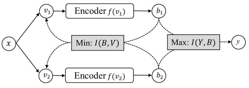
Figure 1: Illustration of the training procedures of CIBHash. An encoder $f(\cdot)$ is trained via maximizing distinctive semantic information, i.e., $Max:I(Y,B)$; and simultaneously minimizing superfluous information, i.e., $Min:I(B,V)$.

Information bottleneck (IB) is to maximize the mutual information between the representations and output labels, subjecting to some constraint Tishby et al. (2000). That is, it seeks to maximize the objective function

$$R_{IB}=I(Y,B)-\beta I(B,V),$$ (21)

where $\beta$ is a Lagrange multiplier that controls the trade-off between the two types of mutual information; and $V$ denotes the random variable of inputs. Obviously, from the perspective of maximizing mutual information, the proposed probabilistic hashing method can be understood under the IB framework by setting the parameter $\beta$ to $0$. It is widely reported that the parameter $\beta$ can control the amount of information that is dropped from the raw inputs $v$, and if an appropriate value is selected, better semantic representations can be obtained Alemi et al. (2017). Therefore, we can train the proposed hashing model under the broader IB framework by taking the term $I(B,V)$ into account.

Instead of directly maximizing $R_{IB}$, we seek to maximize its lower bound due to the computational intractability of $R_{IB}$. For the second term in (21), by definition, we have $I(B,V)={\mathbb{E}}_{{\mathbb{P}}(v)}\left[KL\left({\mathbb{P}}(b|v)||{\mathbb{P}}(b)\right)\right].$ From the non-negativeness of KL-divergence, it can be easily shown that

$$I(B,V)\leq{\mathbb{E}}_{{\mathbb{P}}(v)}\left[KL\left({\mathbb{P}}(b|v)||q(b)\right)\right],$$ (22)

where $q(b)$ could be any distribution of $b$. From (17), we can also get the lower bound for $I(Y,B)$ as $I(Y,B)\geq-L_{ce}+H(Y)$. Thus, we can obtain a lower bound for $R_{IB}$ as

$$R_{IB}\geq-L_{ce}-\beta{\mathbb{E}}_{{\mathbb{P}}(v)}\left[KL\left({\mathbb{P}}(b|v)||q(b)\right)\right]+H(Y).$$ (23)

Since $H(Y)$ is a constant and $L_{ce}$ is exactly the contrastive loss, to optimize the lower bound, we just need to derive the expression for the KL term. By assuming $q(b)$ follows a multivariate Bernoulli distribution $q(b)=Bernoulli(\gamma)$, the expression of KL-divergence $KL\left({\mathbb{P}}(b|v)||q(b)\right)$ can be easily derived to be

In our experiments, for a given view $v_{1}^{(k)}$, the value of $\gamma$ is set by letting $q(b)=p(b|v_{2}^{(k)})$; and $q(b)$ for the view $v_{2}^{(k)}$ can be defined similarly. Intuitively, by encouraging the encoding distributions from different views of the same image close to each other, the model can eliminate superfluous information from each view. In this way, the lower bound of $R_{IB}$ can be maximized by SGD algorithms efficiently. We name the proposed model as CIBHash, standing for Hashing with Contrastive Information Bottleneck. The architecture is shown in Figure 1.

5 Experiments

5.1 Datasets, Evaluation and Baselines

Datasets

Three datasets are used to evaluate the performance of the proposed hashing method. 1) CIFAR-10 is a dataset consisting of $60,000$ images from $10$ classes Krizhevsky and Hinton (2009). We randomly select $1,000$ images per class as the query set and $500$ images per class as the training set, and all the remaining images except queries are used as the database. 2) NUS-WIDE is a multi-label dataset containing $269,648$ images from $81$ categories Chua et al. (2009). Following the commonly used setting, the subset with images from the $21$ most frequent categories is used. We select 100 images per class as the query set and use the remaining as the database. Moreover, we uniformly select $500$ images per class from the database for training, as done in Shen et al. (2020). 3) MSCOCO is a large-scale dataset for object detection, segmentation and captioning Lin et al. (2014). Same as the previous works, a subset of $122,218$ images from $80$ categories is considered. We randomly select $5,000$ images from the subset as the query set and use the remaining images as the database. $10,000$ images from the database are randomly selected for training.

Evaluation Metric

In our experiments, the mean average precision (MAP) at top $N$ is used to measure the quality of obtained hashing codes. Following the settings in Cao et al. (2017); Shen et al. (2020), we adopt MAP@1000 for CIFAR-10, MAP@5000 for NUS-WIDE and MSCOCO.

Baselines

In this work, we consider the following unsupervised deep hashing methods for comparison: DeepBit Lin et al. (2016), SGH Dai et al. (2017), BGAN Song et al. (2018), BinGAN Zieba et al. (2018), GreedyHash Su et al. (2018), HashGAN Dizaji et al. (2018), DVB Shen et al. (2019), and TBH Shen et al. (2020). For the reported performance of baselines, they are quoted from TBH Shen et al. (2020).

5.2 Training Details

For images from the three datasets, they are all resized to $224\times 224\times 3$. Same as the original contrastive learning Chen et al. (2020), during training the resized images are transformed into different views with transformations like random cropping, random color distortions and Gaussian blur, and then are input into the encoder network. In our experiments, the encoder network $f_{\theta}(\cdot)$ is constituted by a pre-trained VGG-16 network Simonyan and Zisserman (2015) followed by an one-layer ReLU feedforward neural network with 1024 hidden units. During the training, following previous works Su et al. (2018); Shen et al. (2019), we fix the parameters of pre-trained VGG-16 network, while only training the newly added feedfoward neural network. We implement our model on PyTorch and employ the optimizer Adam for optimization, in which the default parameters are used and the learning rate is set to be $0.001$. The temperature $\tau$ is set to $0.3$, and $\beta$ is set to $0.001$.

Table 1: MAP comparison with different state-of-the-art unsupervised hashing methods.

Method	Reference	CIFAR-10			NUS-WIDE			MSCOCO
		16bits	32bits	64bits	16bits	32bits	64bits	16bits	32bits	64bits
DeepBit	CVPR16	0.194	0.249	0.277	0.392	0.403	0.429	0.407	0.419	0.430
SGH	ICML17	0.435	0.437	0.433	0.593	0.590	0.607	0.594	0.610	0.618
BGAN	AAAI18	0.525	0.531	0.562	0.684	0.714	0.730	0.645	0.682	0.707
BinGAN	NIPS18	0.476	0.512	0.520	0.654	0.709	0.713	0.651	0.673	0.696
GreedyHash	NIPS18	0.448	0.473	0.501	0.633	0.691	0.731	0.582	0.668	0.710
HashGAN	CVPR18	0.447	0.463	0.481	-	-	-	-	-	-
DVB	IJCV19	0.403	0.422	0.446	0.604	0.632	0.665	0.570	0.629	0.623
TBH	CVPR20	0.532	0.573	0.578	0.717	0.725	0.735	0.706	0.735	0.722
CIBHash	Ours	0.590	0.622	0.641	0.790	0.807	0.815	0.737	0.760	0.775

Table 2: MAP comparison with variants of CIBHash.

Component Analysis		16bits	32bits	64bits
CIFAR-10	Naive CL	0.493	0.574	0.606
	CLHash	0.584	0.612	0.633
	CIBHash	0.590	0.622	0.641
MSCOCO	Naive CL	0.666	0.712	0.737
	CLHash	0.725	0.753	0.765
	CIBHash	0.737	0.760	0.775

5.3 Results and Analysis

Overall Performance

Table 1 presents the performances of our proposed model CIBHash on three public datasets with code lengths varying from $16$ to $64$. For comparison, the performance of baseline models is also included. From the table, it can be seen that the proposed CIBHash model outperforms the current SOTA method by a substantial margin on all three datasets considered. Specifically, an averaged improvement of $5.7\%$, $7.8\%$, $3.6\%$ (averaged over different code lengths) on CIFAR-10, NUS-WIDE, and MSCOCO datasets are observed, respectively, when it is compared to the currently best performed method TBH. The gains are even more obvious on the short code case. All of these reveal that the non-reconstruction-based hashing method is really better at extracting important semantic information than the reconstruction-based ones. This also reveals that when contrastive learning is placed under the information bottleneck framework, high-quality hashing codes can be learned. For more comparisons and results, please refer to Supplementary Materials.

Component Analysis

To understand the influence of different components in CIBHash, we further evaluate the performance of two variants of our model. (i) Naive CL: It produces hashing codes by directly binarizing the real-valued representations learned under the original contrastive learning framework using the median value as the threshold. (ii) CLHash: CLHash denotes the end-to-end probabilistic hashing model derived from contrastive learning, as proposed in Section 3.2. As seen from Table 2, compared to Naive CL, CLHash improves the averaged performance by $5.2\%$ ,$4.3\%$ on CIFAR-10 and MSCOCO, respectively, which demonstrates the effectiveness of our proposed adaptations on the original contrastive learning, i.e., dropping the projection head and enabling end-to-end training. If we compare CIBHash to CLHash, improvements of $0.8\%$ and $1.0\%$ can be further observed on CIFAR-10 and MSCOCO, respectively, which fully corroborates the advantages of considering the CLHash under the broader IB framework.

Table 3: MAP comparison with different IB-based methods.

Method	CIFAR-10
	16bits	32bits	64bits
$\beta$-VAE	0.468	0.508	0.495
Multi-View $\beta$-VAE	0.465	0.492	0.522
CIBHash	0.590	0.622	0.641

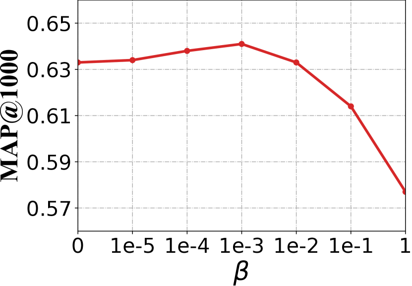
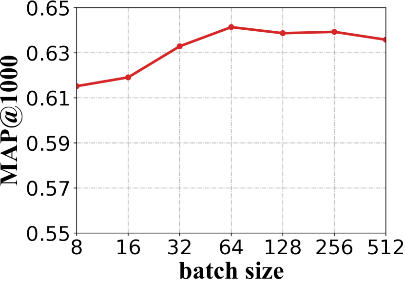
Figure 2: Parameter analysis for the Lagrange multiplier $\beta$ and the batch size with 64-bit hashing codes on CIFAR-10.

Parameter Analysis

To see how the key hyperparameters $\beta$ and minibatch size influence the performance, we evaluate the model under different $\beta$ values and minibatch sizes. As shown in the left column of Figure 2, the parameter $\beta$ plays an important role in obtaining good performance. If it is set too small or too large, the best performance cannot be obtained under either case. Then, due to the observed gains of using large batch sizes in the original contrastive learning, we also study the effect of batch sizes in our proposed CIBHash model. The results are presented in the right column of Figure 2. We see that as the batch size increases, the performance rises steadily at first and then converges to some certain level when the batch size is larger than $64$.

Comparison with $\beta$-VAE

$\beta$-VAE can be regarded as an unsupervised representation learning method under the IB framework Alemi et al. (2017), where $\beta$ controls the relative importance of reconstruction error and data compression. The main difference between $\beta$-VAE and our model CIBHash is that $\beta$-VAE relies on reconstruction to learn representations, while our model leverages contrastive learning that maximizes the agreement between different views of an image. We evaluate the $\beta$-VAE and multi-view $\beta$-VAE. Table 3 shows that CIBHash dramatically outperforms both methods. This proves that the non-reconstruction-based method is better at extracting semantic information than the reconstruction-based methods again.

6 Conclusion

In this paper, we proposed a novel non-reconstruction-based unsupervised hashing method, namely CIBHash. In CIBHash, we attempted to adapt the contrastive learning to the task of hashing, by which its original structure was modified and a probabilistic Bernoulli representation layer was introduced to the model, thus enabling the end-to-end training. By viewing the proposed model under the broader IB framework, a more general hashing method is obtained. Extensive experiments have shown that CIBHash significantly outperformed existing unsupervised hashing methods.

Appendix A Comparison with Non-Deep Hashing Methods

We compare CIBHash with several non-deep unsupervised hashing methods, including ITQ Gong et al. [2013], SH Weiss et al. [2008], SpH Heo et al. [2012], LSH Charikar [2002], SELVE Zhu et al. [2014], AGH Liu et al. [2011] and DGH Liu et al. [2014].

Following the setting in Shen et al. [2019], we randomly select $100$ images from each class on CIFAR-10 as the query set and use the rest $59,000$ images as the database. $500$ images per class in the database are adopted as the training set. For the reported performance of these baselines, they are quoted from Shen et al. [2019]. As shown in Table 4, our CIBHash consistently outperforms these non-deep hashing methods.

Table 4: MAP@All comparison with different non-deep hashing methods on CIFAR-10.

Method	CIFAR-10
	16bits	32bits	64bits
ITQ	0.319	0.334	0.347
SH	0.218	0.198	0.181
SpH	0.229	0.253	0.283
LSH	0.163	0.182	0.232
SELVE	0.309	0.281	0.239
AGH	0.301	0.270	0.238
DGH	0.332	0.354	0.356
CIBHash(Ours)	0.397	0.421	0.442

Appendix B More Performance Comparisons

Precision@1000

Precision@N is defined as the average ratio of similar instances among the top N returned instances of all queries in terms of Hamming Distance. We also use Precision@1000 to evaluate the performance of our CIBHash on CIFAR-10 and MSCOCO. Table 5 shows that CIBHash consistently outperforms other state-of-the-art methods.

Table 5: Precision@1000 comparision with different methods.

Method	CIFAR-10			MSCOCO
	16bits	32bits	64bits	16bits	32bits	64bits
HashGAN	0.418	0.436	0.455	-	-	-
SGH	0.387	0.380	0.367	0.604	0.615	0.637
GreedyHash	0.322	0.403	0.444	0.603	0.624	0.675
TBH	0.497	0.524	0.529	0.646	0.698	0.701
CIBHash(Ours)	0.526	0.570	0.583	0.734	0.767	0.785

Precision-Recall Curve

The Precision-Recall(P-R) curve is based on hash lookup. Figure 4 shows the P-R curve on CIFAR-10. As can be seen from the result, our retrieval performance is obviously better than that of TBH and GreedyHash.

Appendix C Influence of Different Temperature

We further study the influence of the hyperparameter $\tau$. Figure 3 shows the effect of $\tau$ on CIFAR-10 dataset. We fix $\beta$ to 0.001 and evaluate the MAP by varying $\tau$ between 0.1 and 1. The performance shows that our model performs relatively better with $\tau$ between 0.2 and 0.6.

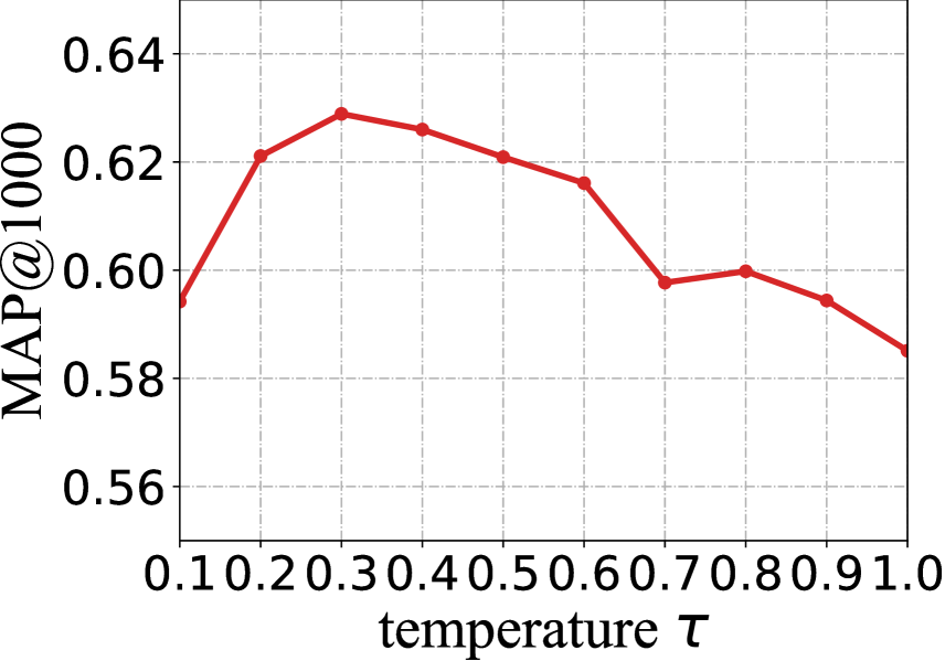
Figure 3: Model performance with various temperature $\tau$ in terms of 32bits on CIFAR-10.

Appendix D Visualization

Case Analysis

As shown in Figure 5, most labels of top-10 return images share the same category with queries, demonstrating the superiority of our CIBHash.

t-SNE Projection

To intuitively investigate the performance of our CIBHash, we project the 32-bit hashing codes on CIFAR-10 into a 2-dimensional plane. As shown in Figure 6, the hashing codes produced by our CIBHash are more distinguishable when compared with those generated from TBH.

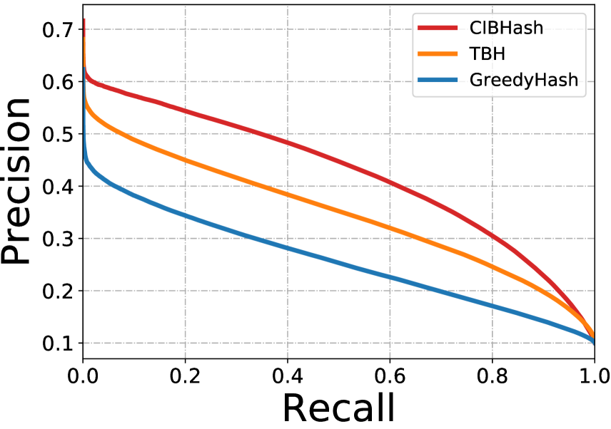
(a) 16 bits

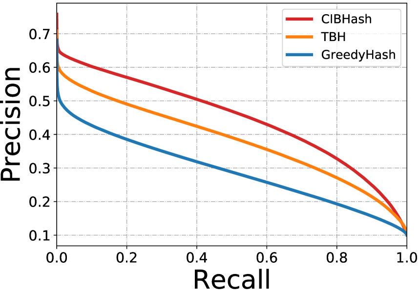
(b) 32 bits

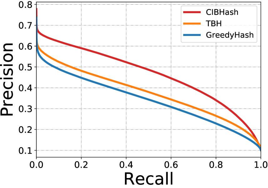
(c) 64 bits

Figure 4: Precision-Recall curves on CIFAR-10.

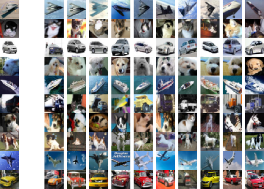
Figure 5: 64-bit retrieval results on CIFAR-10.

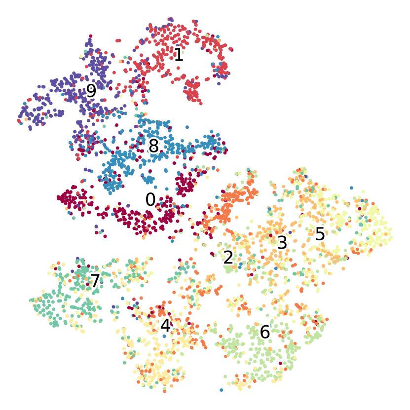
(a) CIBHash

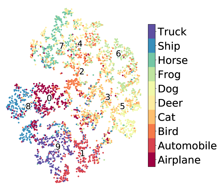
(b) TBH

Figure 6: Visualization of the 32-bit hashing codes generated by CIBHash and TBH on CIFAR-10.

References

- Alemi et al. [2017] Alexander A. Alemi, Ian Fischer, Joshua V. Dillon, and Kevin Murphy. Deep variational information bottleneck. In ICLR (Poster), 2017.
- Baluja and Covell [2008] Shumeet Baluja and Michele Covell. Learning to hash: forgiving hash functions and applications. Data Min. Knowl. Discov., 17(3):402–430, 2008.
- Bengio et al. [2013] Yoshua Bengio, Nicholas Léonard, and Aaron C. Courville. Estimating or propagating gradients through stochastic neurons for conditional computation. CoRR, abs/1308.3432, 2013.
- Cao et al. [2017] Zhangjie Cao, Mingsheng Long, Jianmin Wang, and Philip S. Yu. Hashnet: Deep learning to hash by continuation. In ICCV, pages 5609–5618, 2017.
- Charikar [2002] Moses Charikar. Similarity estimation techniques from rounding algorithms. In STOC, pages 380–388. ACM, 2002.
- Chen et al. [2020] Ting Chen, Simon Kornblith, Mohammad Norouzi, and Geoffrey E. Hinton. A simple framework for contrastive learning of visual representations. In ICML, pages 1597–1607, 2020.
- Chua et al. [2009] Tat-Seng Chua, Jinhui Tang, Richang Hong, Haojie Li, Zhiping Luo, and Yantao Zheng. NUS-WIDE: a real-world web image database from national university of singapore. In CIVR, 2009.
- Dai et al. [2017] Bo Dai, Ruiqi Guo, Sanjiv Kumar, Niao He, and Le Song. Stochastic generative hashing. In ICML, volume 70 of Proceedings of Machine Learning Research, pages 913–922, 2017.
- Dizaji et al. [2018] Kamran Ghasedi Dizaji, Feng Zheng, Najmeh Sadoughi, Yanhua Yang, Cheng Deng, and Heng Huang. Unsupervised deep generative adversarial hashing network. In CVPR, pages 3664–3673, 2018.
- Do et al. [2016] Thanh-Toan Do, Anh-Dzung Doan, and Ngai-Man Cheung. Learning to hash with binary deep neural network. In European Conference on Computer Vision, pages 219–234. Springer, 2016.
- Dong et al. [2019] Wei Dong, Qinliang Su, Dinghan Shen, and Changyou Chen. Document hashing with mixture-prior generative models. In Proceedings of the 2019 Conference on Empirical Methods in Natural Language Processing and the 9th International Joint Conference on Natural Language Processing (EMNLP-IJCNLP), pages 5229–5238, 2019.
- Federici et al. [2020] Marco Federici, Anjan Dutta, Patrick Forré, Nate Kushman, and Zeynep Akata. Learning robust representations via multi-view information bottleneck. In ICLR, 2020.
- Gong et al. [2013] Yunchao Gong, Svetlana Lazebnik, Albert Gordo, and Florent Perronnin. Iterative quantization: A procrustean approach to learning binary codes for large-scale image retrieval. IEEE Trans. Pattern Anal. Mach. Intell., 35(12):2916–2929, 2013.
- Grill et al. [2020] Jean-Bastien Grill, Florian Strub, Florent Altché, Corentin Tallec, Pierre H. Richemond, Elena Buchatskaya, Carl Doersch, Bernardo Ávila Pires, Zhaohan Guo, Mohammad Gheshlaghi Azar, Bilal Piot, Koray Kavukcuoglu, Rémi Munos, and Michal Valko. Bootstrap your own latent - A new approach to self-supervised learning. In NeurIPS, 2020.
- He et al. [2020] Kaiming He, Haoqi Fan, Yuxin Wu, Saining Xie, and Ross B. Girshick. Momentum contrast for unsupervised visual representation learning. In CVPR, pages 9726–9735, 2020.
- Heo et al. [2012] Jae-Pil Heo, Youngwoon Lee, Junfeng He, Shih-Fu Chang, and Sung-Eui Yoon. Spherical hashing. In CVPR, pages 2957–2964. IEEE Computer Society, 2012.
- Hinton et al. [2015] Geoffrey E. Hinton, Oriol Vinyals, and Jeffrey Dean. Distilling the knowledge in a neural network. CoRR, abs/1503.02531, 2015.
- Huang et al. [2017] Shanshan Huang, Yichao Xiong, Ya Zhang, and Jia Wang. Unsupervised triplet hashing for fast image retrieval. In ACM Multimedia (Thematic Workshops), pages 84–92, 2017.
- Krizhevsky and Hinton [2009] A. Krizhevsky and G. Hinton. Learning multiple layers of features from tiny images. Handbook of Systemic Autoimmune Diseases, 1(4), 2009.
- Lew et al. [2006] Michael S Lew, Nicu Sebe, Chabane Djeraba, and Ramesh Jain. Content-based multimedia information retrieval: State of the art and challenges. ACM Transactions on Multimedia Computing, Communications, and Applications (TOMM), 2(1):1–19, 2006.
- Lin et al. [2014] Tsung-Yi Lin, Michael Maire, Serge Belongie, James Hays, Pietro Perona, Deva Ramanan, Piotr Dollár, and C Lawrence Zitnick. Microsoft coco: Common objects in context. In European conference on computer vision, pages 740–755. Springer, 2014.
- Lin et al. [2016] Kevin Lin, Jiwen Lu, Chu-Song Chen, and Jie Zhou. Learning compact binary descriptors with unsupervised deep neural networks. In CVPR, pages 1183–1192, 2016.
- Liu et al. [2011] Wei Liu, Jun Wang, Sanjiv Kumar, and Shih-Fu Chang. Hashing with graphs. In ICML, pages 1–8, 2011.
- Liu et al. [2014] Wei Liu, Cun Mu, Sanjiv Kumar, and Shih-Fu Chang. Discrete graph hashing. In NIPS, pages 3419–3427, 2014.
- Maddison et al. [2017] Chris J. Maddison, Andriy Mnih, and Yee Whye Teh. The concrete distribution: A continuous relaxation of discrete random variables. In ICLR (Poster), 2017.
- Shen et al. [2018] Dinghan Shen, Qinliang Su, Paidamoyo Chapfuwa, Wenlin Wang, Guoyin Wang, Ricardo Henao, and Lawrence Carin. Nash: Toward end-to-end neural architecture for generative semantic hashing. In Proceedings of the 56th Annual Meeting of the Association for Computational Linguistics (Volume 1: Long Papers), pages 2041–2050, 2018.
- Shen et al. [2019] Yuming Shen, Li Liu, and Ling Shao. Unsupervised binary representation learning with deep variational networks. Int. J. Comput. Vis., 127(11-12):1614–1628, 2019.
- Shen et al. [2020] Yuming Shen, Jie Qin, Jiaxin Chen, Mengyang Yu, Li Liu, Fan Zhu, Fumin Shen, and Ling Shao. Auto-encoding twin-bottleneck hashing. In CVPR, pages 2815–2824, 2020.
- Simonyan and Zisserman [2015] Karen Simonyan and Andrew Zisserman. Very deep convolutional networks for large-scale image recognition. In ICLR, 2015.
- Song et al. [2018] Jingkuan Song, Tao He, Lianli Gao, Xing Xu, Alan Hanjalic, and Heng Tao Shen. Binary generative adversarial networks for image retrieval. In AAAI, pages 394–401, 2018.
- Su et al. [2018] Shupeng Su, Chao Zhang, Kai Han, and Yonghong Tian. Greedy hash: Towards fast optimization for accurate hash coding in CNN. In NeurIPS, pages 806–815, 2018.
- Tishby et al. [2000] Naftali Tishby, Fernando C Pereira, and William Bialek. The information bottleneck method. arXiv preprint physics/0004057, 2000.
- Weiss et al. [2008] Yair Weiss, Antonio Torralba, and Robert Fergus. Spectral hashing. In NIPS, pages 1753–1760. Curran Associates, Inc., 2008.
- Yang et al. [2018] Erkun Yang, Cheng Deng, Tongliang Liu, Wei Liu, and Dacheng Tao. Semantic structure-based unsupervised deep hashing. In IJCAI, pages 1064–1070, 2018.
- Yang et al. [2019] Erkun Yang, Tongliang Liu, Cheng Deng, Wei Liu, and Dacheng Tao. Distillhash: Unsupervised deep hashing by distilling data pairs. In CVPR, pages 2946–2955, 2019.
- Zheng et al. [2020] Lin Zheng, Qinliang Su, Dinghan Shen, and Changyou Chen. Generative semantic hashing enhanced via boltzmann machines. In Proceedings of the 58th Annual Meeting of the Association for Computational Linguistics, pages 777–788, 2020.
- Zhu et al. [2014] Xiaofeng Zhu, Lei Zhang, and Zi Huang. A sparse embedding and least variance encoding approach to hashing. IEEE Trans. Image Process., 23(9):3737–3750, 2014.
- Zieba et al. [2018] Maciej Zieba, Piotr Semberecki, Tarek El-Gaaly, and Tomasz Trzcinski. Bingan: Learning compact binary descriptors with a regularized GAN. In NeurIPS, pages 3612–3622, 2018.