3D Restoration of sedimentary terrains: The GeoChron Approach

Abstract

Three-dimensional restoration of complex structural models has become a recognized validation method. Bringing a sedimentary structural model back in time to various deposition stages may also help understand the geological history of a study area and follow the evolution of potential hydrocarbon source rocks, reservoirs and closures.

Most current restoration methods rely on finite-element codes which require a mesh that conforms to both horizons and faults, a difficult object to generate in complex structural settings. Some innovative approaches use implicit horizon representations to circumvent meshing requirements. In all cases, finite-element restoration codes depend on elasticity theory which relies on mechanical parameters to characterize rock behavior during the physical unfolding process.

In this paper, we present a geometric restoration method based on the mathematical theory provided by the GeoChron framework. No assumption is made on the extent of deformation, nor on the nature of terrains being restored. Equations derived from the theory developed for the GeoChron model ensure model consistency at each restored stage.

As the only essential input is a GeoChron model, this restoration technique does not require any specialist knowledge and can be included in any existing structural model-building workflow as a standard validation tool. A model can quickly be restored to any desired stage without providing input mechanical parameters for each layer nor defining boundary conditions, enabling geologists to iterate on the structural model and refine their interpretations until they are satisfied with both input and restored models.

1 Introduction

Many computerized methods have been developed in the past 30 years to build numerical models of sedimentary terrains from seismic and well data, where geological layers are often both folded and faulted. Estimations and forecasts based on such models may impact economic decisions, so numerical representations of available data must be as accurate and consistent as possible.

One way of checking whether any sub-surface model is consistent is to bring it back in time, to a state prior to faulting and folding for a given geological horizon (Moretti,, 2008; Maerten and Maerten,, 2015). If such a process fails, the incriminated areas may point out inconsistencies in the present-day structural model. If it is successful, the geologist can use this simpler restored model to refine his interpretations and build a geological history of the study area (Durand-Riard et al.,, 2013).

Most 3D geological restoration techniques based on mechanics of continuous media assume that geological layers deform in a linear elastic manner (Maerten and Maerten,, 2015). However, the faulted subsurface is a discontinuous medium in which large, non-linear plastic deformations occur. Large deformations are taken into account by some restoration methods (e.g. Muron, (2005); Moretti et al., (2006)) but induce a time-consuming, heavy computation load for each restored stage. Moreover, mechanical restoration methods may result in restored models with gaps and overlaps close to fault-induced discontinuities, which are then minimized through debatable numerical post-processes.

Lovely et al., (2018) present a simple, purely geometrical restoration method based on the commercially available implementation of the GeoChron theory (Mallet,, 2014) provided by Emerson Paradigm^® in the SKUA^™ software package. In this paper, we derive a full geometrical restoration theory from the fundamental equations of the GeoChron model and show complete implementation results. For input GeoChron models of any degree of geometrical and topological complexity, our method handles both small and large deformations, does not assume elastic behavior and does not require any prior knowledge of geo-mechanical properties. Finally, the fundamental equations of this method intrinsically integrate minimization of gaps and overlaps along faults without any need for post-processing.

2 Overview of the mathematical GeoChron framework

This section briefly describes the main elements of the mathematical GeoChron framework used in this article. The complete theory may be found in Mallet, (2014).

As illustrated by Figure 1, consider a geo-stationary satellite pointing a camera vertically towards a region of interest on the surface of the Earth. This camera delimits a right-handed frame of three orthogonal unit vectors $\{\bar{\bf r}_{u},\bar{\bf r}_{v},\bar{\bf r}_{t}\}$ where $\bar{\bf r}_{t}$ is orthogonal to the surface of the Earth and oriented upward. These three vectors define the edges of a box where images shot by the camera are stacked in chronological order throughout geological-time. For coherency with the geological processes, the camera is geo-stationary in the sense that its origin and $\{\bar{\bf r}_{u},\bar{\bf r}_{v},\bar{\bf r}_{t}\}$ vectors are “attached” to the tectonic plate which contains the domain of interest.

Figure 1: $\overline{G}$-space viewed as a continuous chronological stack of images $\{\overline{H}_{t}\}$ of the surface of the Earth shot from a geo-stationary camera throughout geological-time (in Mallet, (2014), courtesy of EAGE).

Let $\overline{H}_{\tau}$ be a horizontal plane orthogonal to the vector $\bar{\bf r}_{t}$ and corresponding to the one-to-one map of the sea floor at geological-time $\tau$. $\overline{H}_{\tau}$ is identical to a picture of the sea floor taken at geological-time $\tau$ and is therefore parallel to the pair of orthogonal unit vectors $\{\bar{\bf r}_{u},\bar{\bf r}_{v}\}$, which can thus be used as a 2D frame for $\overline{H}_{\tau}$. As a consequence, for any given origin $\bar{\bf p}_{0}(t)$ belonging to $\overline{H}_{\tau}$, the pair of vectors $\{\bar{\bf r}_{u},\bar{\bf r}_{v}\}$ induces a rectilinear coordinate system $(u,v)$ on $\overline{H}_{\tau}$ such that:

$$\bar{\bf p}\in\overline{H}_{\tau}\quad\Longleftrightarrow\quad\exists\ (u,v)\in{I\!\!R}^{2}\ :\ \bar{\bf p}\ =\ \bar{\bf p}_{0}(\tau)+u\cdot\bar{\bf r}_{u}+v\cdot\bar{\bf r}_{v}$$ (1)

At geological-time $\tau$, the $(u,v)$ rectilinear coordinate system so defined can thus be used to locate on map $\overline{H}_{\tau}$ any particle of sediment being deposited at that geological-time. Therefore, the $(u,v)$ pair is called “paleo-geographic coordinate” system. On sea floor $H_{\tau}$, the reverse image of the rectilinear coordinate axes $(u)$ and $(v)$ consists in a curvilinear coordinate system.

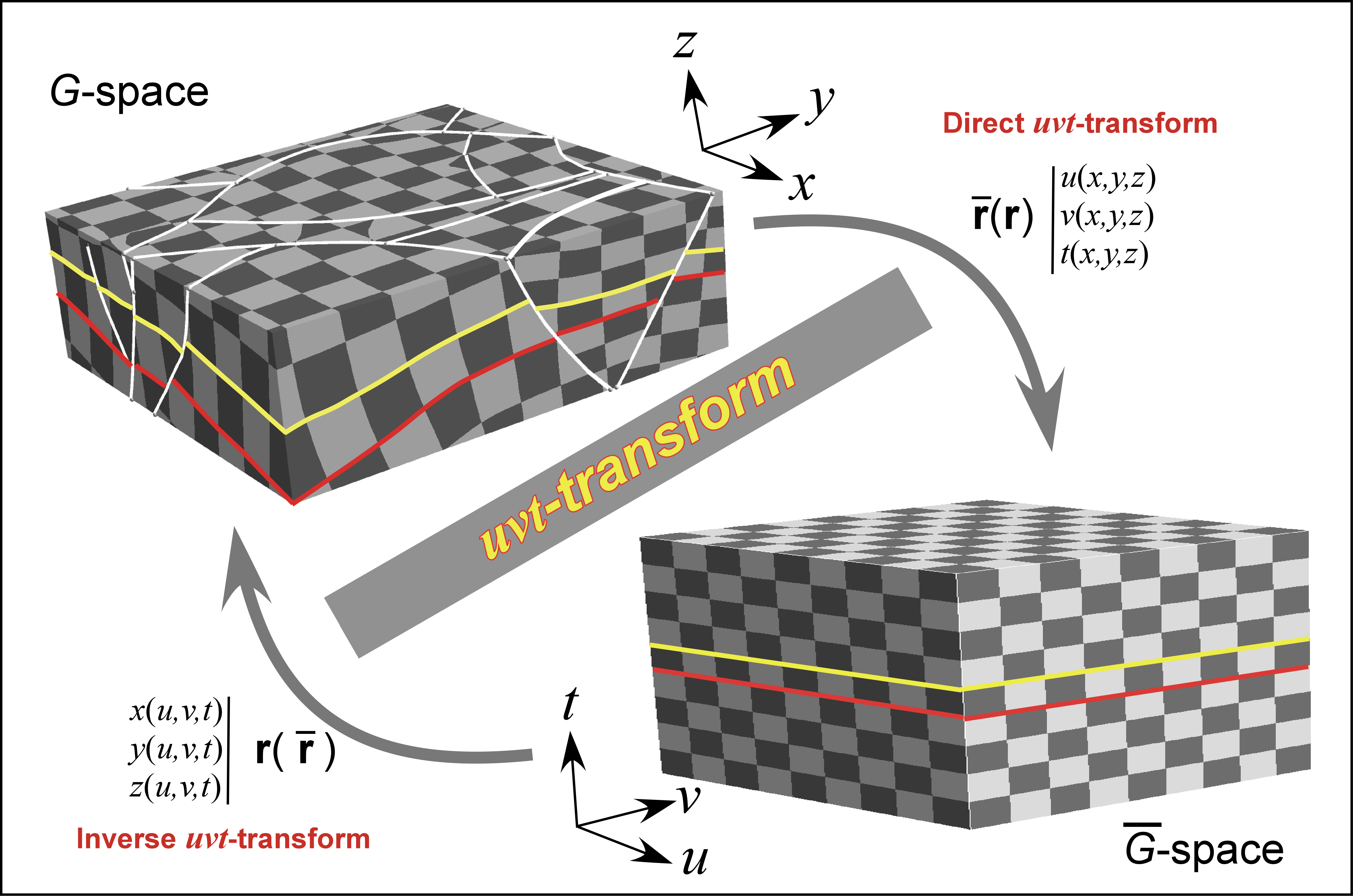
Figure 2: Graphical characterization of direct and inverse $uvt$-transforms (in Mallet, (2014), courtesy of EAGE).

Let $G$, also called $G$-space, be the domain of interest in stratified sedimentary terrains. Two distinct coordinate systems characterize any particle of sediment observed today at location ${\bf r}\in G$ in the subsurface:

• First, present-day horizontal geographic coordinates $\{x({\bf r}),y({\bf r})\}$ and altitude $z({\bf r})$ with respect to a given direct 3D frame consisting of three orthogonal unit vectors $\{{\bf r}_{x},{\bf r}_{y},{\bf r}_{z}\}$ associated with the $G$-space, where ${\bf r}_{z}$ is vertical and oriented upward:

  $${\bf r}\ =\ x({\bf r})\cdot{\bf r}_{x}+y({\bf r})\cdot{\bf r}_{y}+z({\bf r})\cdot{\bf r}_{z}\quad\in G$$ (2)

• Second, paleo-geographic coordinates $\{u({\bf r}),v({\bf r})\}$ as they could have been observed at geological-time $t({\bf r})$ when the particle was deposited. These paleo-coordinates $\{u({\bf r}),v({\bf r}),t({\bf r})\}$ define the location $\overline{{\bf r}}$ of the particle in a “depositional” space $\overline{G}$ also called $\overline{G}$-space:

  $$\overline{{\bf r}}\ =\ u({\bf r})\cdot\overline{{\bf r}}_{u}+v({\bf r})\cdot\overline{{\bf r}}_{v}+t({\bf r})\cdot\overline{{\bf r}}_{t}\quad\in\overline{G}$$ (3)

  In this definition, the $\overline{G}$-space is associated with a given, direct 3D frame of three unit orthogonal vectors $\{\overline{{\bf r}}_{u},\overline{{\bf r}}_{v},\overline{{\bf r}}_{t}\}$ where $\overline{{\bf r}}_{t}$ is vertical and oriented upward. From now on, $\overline{G}$ is identified with the box associated with the camera shown in Figure 1.

As Figure 2 shows, the equations above can be viewed as a “direct” $uvt$-transform of point ${\bf r}\in G$ into a point $\overline{{\bf r}}=\overline{{\bf r}}({\bf r})\in\overline{G}$ and, conversely, a “reverse” $uvt$-transform of point $\overline{{\bf r}}\in\overline{G}$ into a point ${\bf r}={\bf r}(\overline{{\bf r}})\in G$. Furthermore, the $uvt$-transform also applies as follows to any function $\varphi$ defined in $G$:

$$\overline{\varphi}(\overline{{\bf r}})=\varphi({\bf r})\quad\forall\>{\bf r}\in G$$ (4)

This concept of $uvt$-transform both of points and functions plays a central role in the GeoChron-based restoration method presented in this article. When referring to a function $\varphi$ defined in $G$, the following notations may be used interchangeably for clarity:

$$\begin{array}[]{llllllllllllllll}&\varphi(x,y,z)&\equiv&\varphi({{\bf r}})&\equiv&\varphi\big{(}\ {{\bf r}}(\bar{{\bf r}})\ \big{)}\\ \\ \equiv&\bar{\varphi}(u,v,t)&\equiv&\bar{\varphi}(\bar{{\bf r}})&\equiv&\bar{\varphi}\big{(}\ \bar{{\bf r}}({{\bf r}})\ \big{)}&\equiv&\overline{\varphi({\bf r})}\end{array}$$ (5)

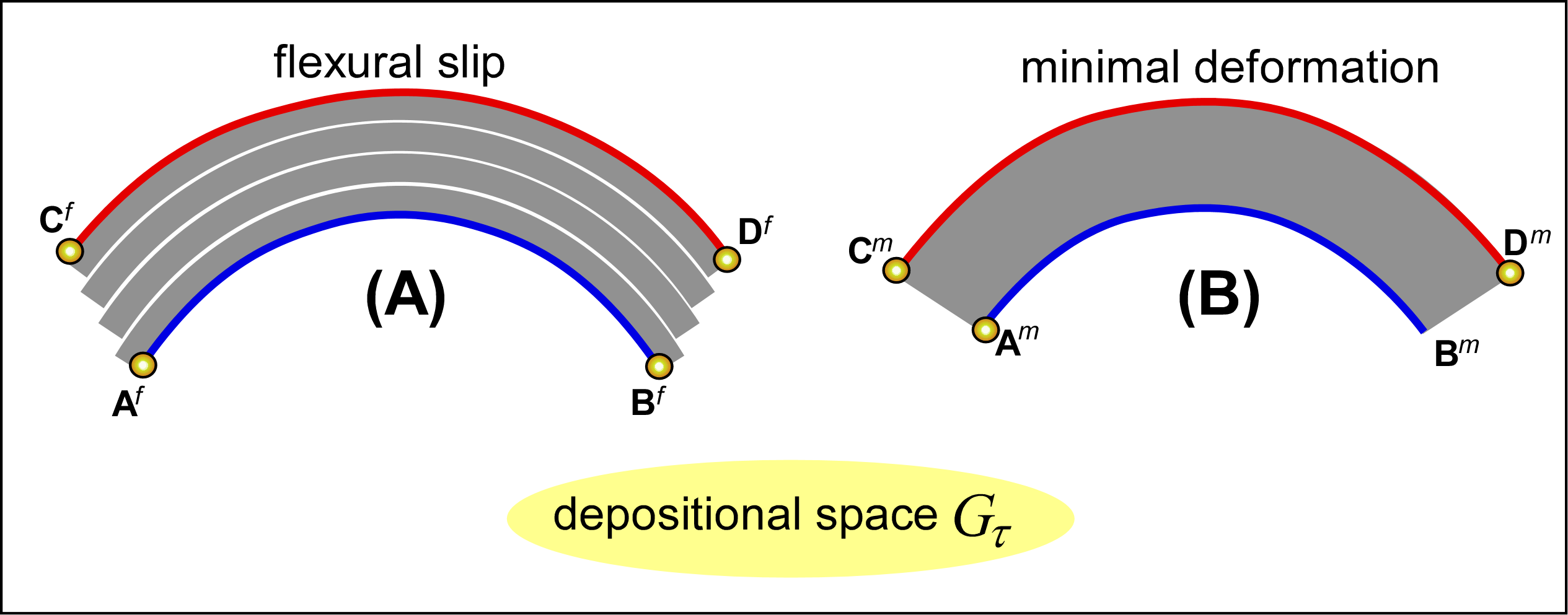
Figure 3: Vertical cross section of a cylindrical, constant thickness layer. If the tectonic style is flexural slip, arc lengths $A^{f}B^{f}$ and $C^{f}D^{f}$ are equal. If the tectonic style is minimal deformation, arc length $A^{m}B^{m}$ is smaller than arc length $C^{m}D^{m}$. As an example, one can picture flexural slip occurring when the material being bent is a stack of paper sheets, but minimal deformation would rather occur with a piece of rubber.

According to geological context, a geologist can choose one of two different tectonic styles to characterize the behavior of geological layers subject to tectonic forces. Figure 3 illustrates both these options, referred to as “flexural slip” and “minimal deformation” (see definitions on pages 53 and 54 of Mallet, (2014)). In the GeoChron framework, these tectonic styles each translate as a different set of equations which constrain the behavior of paleo-geographic coordinates $\{u,v\}$.

Let $\partial_{\alpha}\varphi$ denote $\partial\varphi/\partial\alpha\>\forall\,\alpha\in\{x,y,z\}$ and $\mathbf{grad}\,\varphi$ denote the gradient $\partial_{x}\varphi\,{\bf r}_{x}+\partial_{y}\varphi\,{\bf r}_{y}+\partial_{z}\varphi\,{\bf r}_{z}$ of a function $\varphi$ over frame $\{{\bf r}_{x},{\bf r}_{y},{\bf r}_{z}\}$. The mathematical GeoChron theory presented in (Mallet,, 2014) states that, depending on tectonic style, functions $\{u,v\}_{\bf r}$ are assumed to honor, in a least squares sense, the following differential equations (see pages 70 to 74 in Mallet, (2014)):

$$\begin{array}[]{cc}\mbox{Minimal deformation style:}&\left\{\begin{array}[]{cc}1\&2)&||\mathbf{grad}\,u||\simeq 1\quad;\quad||\mathbf{grad}\,v||\simeq 1\\ \\ 3)&\mathbf{grad}\,u\cdot\mathbf{grad}\,v\ \simeq\ 0\\ 4)&\mathbf{grad}\,t\cdot\mathbf{grad}\,u\ \simeq\ 0\\ 5)&\mathbf{grad}\,t\cdot\mathbf{grad}\,v\ \simeq\ 0\end{array}\right.\end{array}$$ (6)

$$\begin{array}[]{cc}\mbox{Flexural slip style:}&\left\{\begin{array}[]{cccccccc}1\&2)&||\mathbf{grad}_{H}\,u||\simeq 1\quad;\quad||\mathbf{grad}_{H}\,v||\simeq 1\\ \\ 3)&\mathbf{grad}_{H}\,u\cdot\mathbf{grad}_{H}\,v\ \simeq\ 0\end{array}\right.\end{array}$$ (7)

where $\mathbf{grad}\,\varphi({\bf r})$ is the gradient of scalar function $\varphi$ at location ${\bf r}$, $H\equiv H_{t({\bf r})}$ is the horizon passing through point ${{\bf r}\in G}$, defined as the set of particles of sediment which were deposited at geological-time $t({\bf r})$, and $\mathbf{grad}_{H}\,\varphi({{\bf r}})$ is the projection of gradient $\mathbf{grad}\,\varphi({{\bf r}})$ onto said horizon $H$.

Equations 6 or 7 can be honored exactly only in the particular case where horizons are perfectly planar and parallel. In all other cases, local deformations of terrains entail that these equations can only be approximated in a least squares sense. As Figure 2 shows, functions $\{u,v,t\}_{\bf r}$ are continuous and smooth everywhere in $G$ except across faults.

For any equivalent system of GeoChron functions $\{u,v,t\}_{\bf r}$ and any tectonic style, it may be shown that the component ${\cal E}_{\alpha\beta}({\bf r})$ of the strain (deformation) tensor $\mbox{{\boldmath${\cal E}$}}({\bf r})$ at any point ${{\bf r}\in G}$ on the global frame $\{{\bf r}_{x},{\bf r}_{y},{\bf r}_{z}\}$ honors the following equation:

$$2\cdot{\cal E}_{\alpha\beta}({\bf r})\ =\ \delta_{\alpha\beta}\ -\ \biggl{\{}\partial_{\alpha}u\cdot\partial_{\beta}u+\partial_{\alpha}v\cdot\partial_{\beta}v+\frac{N^{\alpha}\cdot N^{\beta}}{(1-\phi)^{2}}\biggr{\}}_{{\bf r}}\qquad\forall\ (\alpha,\beta)\in\{x,y,z\}^{2}$$ (8)

where $\phi({{\bf r}})$ denotes the compaction coefficient at point ${\bf r}$ defined on page 38 of Mallet, (2014) whilst $\{N^{x},N^{y},N^{z}\}_{{\bf r}}$ denote the components on $\{{\bf r}_{x},{\bf r}_{y},{\bf r}_{z}\}$ of the unit vector $\mbox{\bf N}({\bf r})$ orthogonal to horizon $H_{t({\bf r})}$ passing through ${\bf r}$ and oriented in the direction of younger terrains:

$$\mbox{\bf N}({\bf r})\ =\ \frac{\mathbf{grad}\,t({\bf r})}{||\mathbf{grad}\,t({\bf r})||}$$ (9)

3 GeoChron framework for 3D restoration

The restoration method presented in this paper uses as input an initial GeoChron model of the studied domain $G$, which provides (see Figure 4 and Mallet, (2014)):

• Fault network topology and geometry;

  

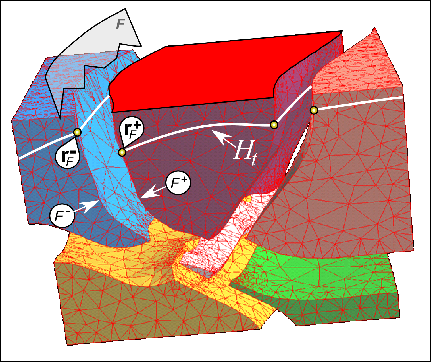
  Figure 4: Exploded view of a faulted, 3D geological domain $G$. During restoration, twin faces $F^{-}$ and $F^{+}$ of fault $F$ must slide on one another. Points $({\bf r}_{\textsc{f}}^{+},{\bf r}_{\textsc{f}}^{-})$, which were collocated on horizon $H_{t}$ at deposition time $t$ prior to faulting, are denoted a pair of “twin-points”.

• For each geological fault $F$, two disconnected surfaces $F^{+}$ and $F^{-}$ bordering $F$ on either side. As observed today, $F^{+}$ and $F^{-}$ are collocated; however, during the restoration process, $F^{+}$ and $F^{-}$ should slide on one another, without generating gaps or overlaps between adjacent fault blocks;

• For each fault $F$, a set of pairs of points $({\bf r}_{\textsc{f}}^{+},{\bf r}_{\textsc{f}}^{-})$ called “twin-points” and such that:

  1. ${\bf r}_{\textsc{f}}^{+}\in F^{+}$ and ${\bf r}_{\textsc{f}}^{-}\in F^{-}$;

  2. Before $F$ induced any movement in the subsurface, the particles of sediment which are observed today at locations ${\bf r}_{\textsc{f}}^{+}$ and ${\bf r}_{\textsc{f}}^{-}$ were collocated.

  During the activation of fault $F$, particles of sediment initially located on $F$ are assumed to slide along apparent fault-striae defined as the shortest path, on $F$, between pairs of twin points $({\bf r}_{\textsc{f}}^{+},{\bf r}_{\textsc{f}}^{-})$ (see example of fault network with fault-striae in Figure 5). From now on and for concision’s sake, “apparent” fault-striae will simply be called “fault-striae”;

• A tectonic style which may be either “minimal deformation” or “flexural slip”;

• A triplet $\{u,v,t\}_{\bf r}$ of piecewise continuous functions defined on the $G$-space such that, for a particle of sediment observed today at location ${\bf r}\in G$, the numerical values $\{u({\bf r}),v({\bf r})\}$ represent the paleo-geographic coordinates of the particle at geological-time $t({\bf r})$ when it was deposited.

Moreover, inherent to the GeoChron model, the following points are of relevance to the restoration method presented in this paper:

• Each geological horizon $H_{\tau}$ is the set of particles of sediment deposited at a given geological-time $\tau$:

  $${\bf r}\in H_{\tau}\quad\Longleftrightarrow\quad t({\bf r})=\tau$$ (10)

  In other words, $H_{\tau}$ is defined as a level-set of the geological-time function $t({\bf r})$;

• Paleo-geographic coordinates functions $\{u,v\}_{\bf r}$ and twin-points are linked by the following equations:

  $$\begin{array}[]{c}\{\ ({\bf r}_{\textsc{f}}^{+},{\bf r}_{\textsc{f}}^{-})\mbox{ is a pair of twin-points }\}\quad\Longleftrightarrow\quad\left\{\begin{array}[]{ccccccc}1)&{\bf r}_{\textsc{f}}^{+}\in F^{+}\ \mbox{ \mbox{\bf\&} }\ {\bf r}_{\textsc{f}}^{-}\in F^{-}\\ \\ 2)&u({\bf r}_{\textsc{f}}^{-})=u({\bf r}_{\textsc{f}}^{+})\\ 3)&v({\bf r}_{\textsc{f}}^{-})=v({\bf r}_{\textsc{f}}^{+})\\ 4)&t({\bf r}_{\textsc{f}}^{-})=t({\bf r}_{\textsc{f}}^{+})\end{array}\right.\end{array}$$ (11)

  As shown in Figure 5, each pair of twin-points $({\bf r}_{\textsc{f}}^{+},{\bf r}_{\textsc{f}}^{-})$ is the intersection of a level set of function $t({\bf r})$ with a fault-stria. As a consequence of constraints 2-3-4 above, fault-striae characterize the paleo-geographic coordinates $\{u,v\}_{\bf r}$, and vice versa;

• Each point ${\bf r}\in G$ is characterized by its coordinates $\{x({\bf r}),y({\bf r}),z({\bf r})\}$ with respect to a direct frame $\{{\bf r}_{x},{\bf r}_{y},{\bf r}_{z}\}$ consisting of three mutually orthogonal unit vectors with ${\bf r}_{z}$ oriented upward;

• At any location ${\bf r}$ in geological domain $G$, the equation ${\bf x}(s|{\bf r})$ of curve ${\cal N}({\bf r})$ passing through ${\bf r}$, denoted “normal-line”, where $s$ is the arc length abscissa along ${\cal N}({\bf r})$, obeys the following differential relationship:

  $$\frac{d{\bf x}(s|{\bf r})}{ds}\ =\ \mbox{\bf N}({\bf x}(s|{\bf r}))$$ (12)

  where $\mbox{\bf N}({\bf r})$ is the unit vector defined by equation 9.

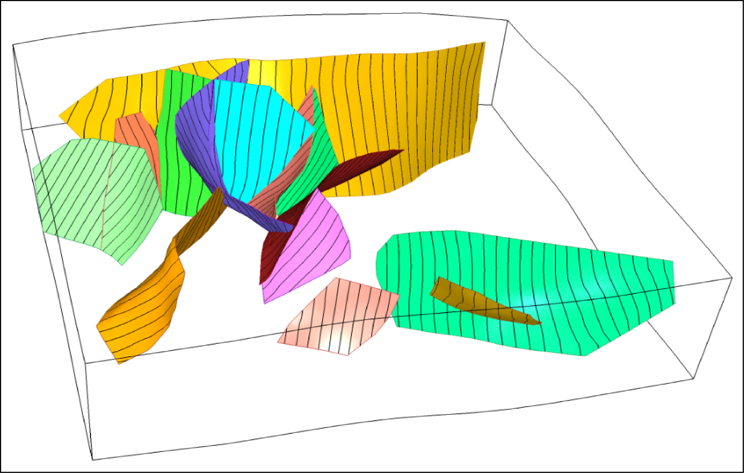
Figure 5: Example of fault-striae drawn on a fault network and deduced from functions $\{u,v,t\}_{\bf r}$ of a GeoChron model. Data courtesy of Total.

Problem to address

Let us assume that, at given geological-time $\tau$, horizon $H_{\tau}$ to be restored coincided with a given, smooth surface $\widetilde{H}_{\tau}$ considered as the sea floor, whose altitude at geological-time $\tau$ is a given function $z_{\tau}^{o}(u,v)$ of GeoChron paleo-geographic coordinates $(u,v)$:

$$\{\ {\bf r}_{\tau}^{o}\in{H}_{\tau}\ \}\quad\Longleftrightarrow\quad\{\ z_{\tau}^{o}({\bf r}_{\tau}^{o})=z_{\tau}^{o}(u({\bf r}_{\tau}^{o}),v({\bf r}_{\tau}^{o}))\ \}$$ (13)

Let $G_{\tau}$ be the part of the $G$-space observed today and geologically deposited up to geological-time $\tau$:

$$\begin{array}[]{|c|}\hline\cr\\ \quad{\bf r}_{\tau}\in G_{\tau}\quad\Longleftrightarrow\quad t({\bf r}_{\tau})\leq\tau\\ \\ \hline\cr\end{array}$$ (14)

The problem then consists in:

1. Restoring horizon $H_{\tau}$ to its initial, unfolded and unfaulted state $\widetilde{H}_{\tau}$ corresponding to sea floor $\widetilde{\cal S}_{\tau}(0)$ at geological-time $\tau$;

2. Reshaping the terrains in such a way that, for each point ${\bf r}_{\tau}\in G_{\tau}$ stratigraphically located below $H_{\tau}$:

   1. the particle of sediment currently located at point ${\bf r}_{\tau}$ moves to its former, restored location $\{\bar{\bf r}_{\tau}=\bar{\bf r}_{\tau}({\bf r}_{\tau})\}$, where it was at geological-time $\tau$;

   2. no overlaps or voids are created in the subsurface;

   3. volume variations are minimized whilst also taking compaction into account.

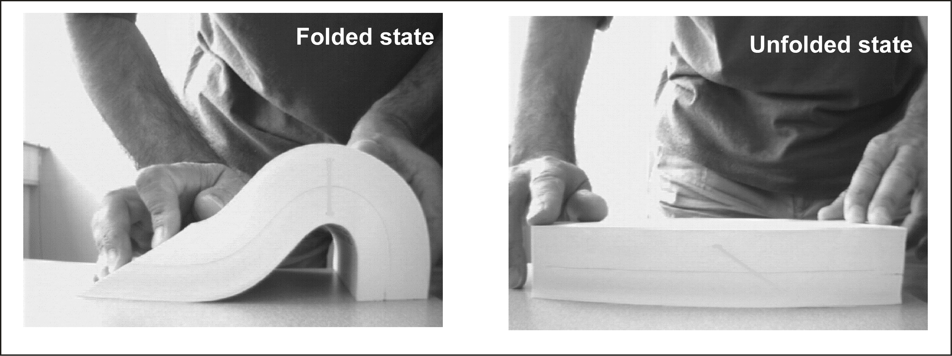
Figure 6: Folding / unfolding a book. Modified after Mallet, (2014).

Comment

Figure 6 shows a book, considered as the analogue of a stack of geological layers, being folded, then laid flat again. Two distinct types of differential equations drive the book’s geometrical transformations:

• Folding:

  1. Initial state:

     • Book pages are parallel and flat, which implies that the book’s initial geometry is known;

     • Mechanical laws which control the behavior of the pages (e.g., elasticity) are known;

     • Physical properties (e.g., Lamé coefficients) of the pages are known;

     • External forces applied to the book are known.

  2. Final state:

     • The book folds under the action of given external forces;

     • Its final geometry may be deduced from the aforementioned mechanical laws and physical properties.

  In this first case, the geometry of the final state is dictated by a set of differential equations controlled by initial geometry and mechanical properties. It seems quite obvious that, with the application of similar external forces, the book’s final geometry will differ considerably according to whether its pages are made of paper, plastic or steel.

• Unfolding:

  1. Initial state:

     • Book pages are folded and their geometry is given;

  2. Final state:

     • The top page of the book is flat and its geometry is given,

     • All book pages remain parallel, without any void or intersection.

  In this second case, the geometry of the final state is dictated by a set of differential equations controlled by initial and final conditions only and does not depend on the pages’ mechanical properties.

This analysis shows that differential equations which rule the folding and unfolding cases differ and do not require the same input and boundary conditions. In particular, unfolding does not require the mechanical properties of the medium (pages of the book) to be known. This is why we state that geologic restoration can be purely geometrical, without relying on geo-mechanical laws and physical properties of geologic layers.

Prior art

Since seminal article Dahlstrom, (1969) was published half a century ago, dozens of methods have been proposed to restore sedimentary terrains as they were at a given geologic time $\tau$ (e.g. Gibbs, (1983); Suppe, (1985); Muron, (2005); Moretti et al., (2006); Moretti, (2008); Maerten and Maerten, (2015)), including some that represent horizons as level-sets of a geological-time function (Durand-Riard et al.,, 2010). So far, only the one developed by Lovely et al., (2018) is based on the GeoChron model paradigm.

Figure 2 illustrates that the $uvt$-transform of the subsurface has the general look of restored stratified terrains. However, this is not true restoration because, in the “unfolded” $\overline{G}$-space, all horizons are transformed into parallel, horizontal planes, so lateral variations in layer thicknesses are generally not preserved.

Note that, barring compaction, in the very particular case where all layers have a constant thickness and the following equation holds

$$||\mathbf{grad}\,t_{\tau}({\bf r}_{\tau})||=1\qquad\forall\ {\bf r}_{\tau}\in G_{\tau}$$ (15)

then, the $uvt_{\tau}$-transform $\overline{G}_{\tau}$ of $G_{\tau}$ preserves the thickness of each layer, which implies that $\overline{G}_{\tau}$ so obtained could be considered as a restored version of $G_{\tau}$. This observation led to the following comment on page 91 in Mallet, (2014), recalled here:

$$\left.\begin{array}[]{c}\mbox{ \begin{minipage}[t]{327.20668pt} \small\sl$\ll$ [\ldots] using a GeoChron model as an \mbox{\bf input}, \\ it is possible to develop new breeds of unfolding algorithms. $\gg$ \end{minipage}\noindent}\end{array}\right.$$

By adding minimal functionalities to commercial SKUA^® software designed to implement the GeoChron model, Lovely et al., (2018) proposed a first, easy to implement restoration algorithm which consists in using classical GeoChron equations to compute restoration functions. These “native” GeoChron equations were not devised with restoration of sedimentary terrains as a goal. Despite this, by clever use of the software, Lovely et al., achieved remarkable first restoration results. As a remedy to some weaknesses their study pointed out, in this paper we adapt the GeoChron model theory, rather than its implementation. The new set of differential equations and boundary conditions obtained as a result are specifically designed to solve geometric restoration problems and provide geologically and geometrically consistent restored models. As we develop each step in our method, we will point out the differences with Lovely et al.,’s work.

4 GeoChron-Based Restoration (GBR)

This section describes a purely geometrical method directly derived from the GeoChron mathematical framework and aimed at restoring terrains at a given geological-time $\tau$, whatever the structural complexity of horizons and faults in studied domain $G$. This GeoChron-Based Restoration (GBR) method can be intuitively introduced by the “jelly block” analogy depicted in Figure 7.

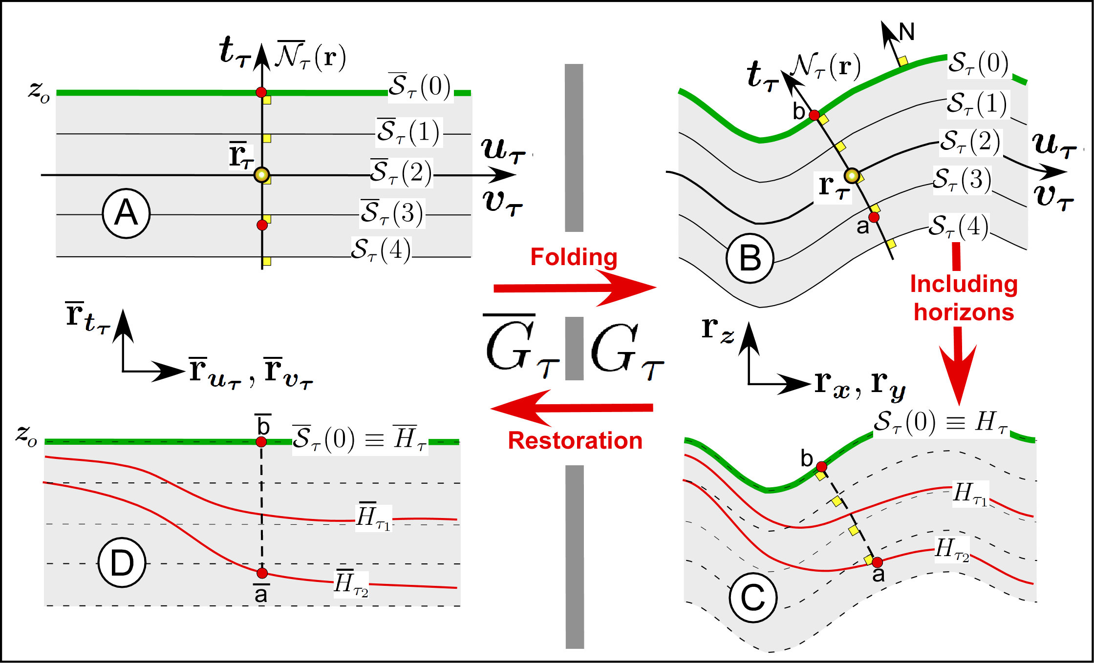
Figure 7: Jelly principle (minimal deformation style): The $u_{\tau}v_{\tau}t_{\tau}$-transform of jelly block $G_{\tau}$ consists of a jelly block $\overline{G}_{\tau}$ identical to the restored version of $G_{\tau}$ as it was at geological-time $\tau$. In Tertois and Mallet, (2019).

Jelly block ${\overline{G}_{\tau}}$

Figure 7-A shows an arbitrarily-shaped “jelly block”, denoted $\overline{G}_{\tau}$, which contains a direct frame of orthogonal unit vectors $\{\bar{\bf r}_{u_{\tau}},\bar{\bf r}_{v_{\tau}},\bar{\bf r}_{t_{\tau}}\}$ and a family of smooth, continuous horizontal surfaces $\{\overline{\cal S}_{\tau}(d):d\geq 0\}$ intersected only once by any vertical straight line parallel to $\bar{\bf r}_{t_{\tau}}$:

1. For each point ${\bar{\bf r}_{\tau}}\in\overline{G}_{\tau}$, $\{u_{\tau}({\bar{\bf r}_{\tau}}),v_{\tau}({\bar{\bf r}_{\tau}})\}$ represent the horizontal coordinates of ${\bar{\bf r}_{\tau}}$ with respect to horizontal unit frame vectors $\{\bar{\bf r}_{u_{\tau}},\bar{\bf r}_{v_{\tau}}\}$ whilst $t_{\tau}(\bar{\bf r}_{\tau})$ represents its altitude with respect to $\bar{\bf r}_{t_{\tau}}$, oriented upward;

2. Any point $\bar{\bf r}_{\tau}^{o}\in\overline{\cal S}_{\tau}(0)$ is located at altitude $(t_{\tau}(\bar{\bf r}_{\tau}^{o})=0)$ with respect to the vertical unit vector $\bar{\bf r}_{t_{\tau}}$ oriented upward;

3. $\overline{\cal S}_{\tau}(d)$ is located at algebraic vertical distance $(d)$ from $\overline{\cal S}_{\tau}(0)$ in such a way that:

   $$\left|\begin{array}[]{cccccccc}d<0&\Longleftrightarrow&\overline{\cal S}_{\tau}(d)&\mbox{is located above }\overline{\cal S}_{\tau}(0)\\ d>0&\Longleftrightarrow&\overline{\cal S}_{\tau}(d)&\mbox{is located below }\overline{\cal S}_{\tau}(0)\end{array}\right.$$ (16)

Contrarily to classical Free Form Deformation methods which, following the principles formulated by Sederberg and Parry, (1986), introduce the concept of jelly block, $\overline{G}_{\tau}$ may be of arbitrary shape and may be discontinuous across surfaces dividing it, either partially or totally.

Jelly block ${G_{\tau}}$

Figure 7-B shows the folded jelly block $G_{\tau}$ resulting from the deformation of jelly block $\overline{G}_{\tau}$ under tectonic forces induced either by minimal deformation or flexural slip tectonic forces:

$$\begin{array}[]{|c|}\hline\cr\\ \quad\begin{array}[]{c}\overline{G}_{\tau}\quad\longrightarrow\mbox{Tectonic forces}\longrightarrow\quad G_{\tau}\end{array}\\ \\ \hline\cr\end{array}$$ (17)

In spaces $\overline{G}_{\tau}$ and $G_{\tau}$:

1. Using reverse and direct $u_{\tau}v_{\tau}t_{\tau}$-transforms, each point ${\bar{\bf r}_{\tau}}\in\overline{G}_{\tau}$ is transformed into point ${\bf r}_{\tau}\in G_{\tau}$, and conversely:

   $${\bar{\bf r}_{\tau}}\in\overline{G}_{\tau}\quad\longleftrightarrow\quad{\bf r}_{\tau}\in G_{\tau}$$ (18)

2. For each point ${\bf r}_{\tau}\in G_{\tau}$:

   • $\{x({\bf r}_{\tau}),y({\bf r}_{\tau})\}$ represent the horizontal geographic coordinates of ${\bf r}_{\tau}$ with respect to $\{{\bf r}_{x},{\bf r}_{y}\}$, whilst $z({\bf r}_{\tau})$ represents its altitude with respect to the vertical unit frame vector ${\bf r}_{z}$ oriented upward;

   • $\{u_{\tau},v_{\tau},t_{\tau}\}_{{\bf r}_{\tau}}$ are functions defined as follows in $G_{\tau}$:

     $$\begin{array}[]{|c|}\hline\cr\\ u_{\tau}({\bf r}_{\tau})=u_{\tau}(\bar{{\bf r}}_{\tau})\quad;\quad v_{\tau}({\bf r}_{\tau})=v_{\tau}(\bar{{\bf r}}_{\tau})\quad;\quad t_{\tau}({\bf r}_{\tau})=t_{\tau}(\bar{{\bf r}}_{\tau})\\ \\ \hline\cr\end{array}$$ (19)

3. Each horizontal surface $\overline{\cal S}_{\tau}(d)\in\overline{G}_{\tau}$ is transformed into a curved surface ${\cal S}_{\tau}(d)\in G_{\tau}$ “parallel” to ${\cal S}_{\tau}(0)$ and each surface ${\cal S}_{\tau}(d)$ is a level-set of function $t_{\tau}({\bf r}_{\tau})$;

4. The images of rectilinear coordinate axes $(u_{\tau})$, $(v_{\tau})$ and $(t_{\tau})$ contained in jelly block $\overline{G}_{\tau}$ consist of curved lines in folded jelly block $G_{\tau}$.

From now on, without loss of generality and for the sake of simplicity, $\overline{G}_{\tau}$-space frame $\{\bar{\bf r}_{u_{\tau}},\bar{\bf r}_{v_{\tau}},\bar{\bf r}_{t_{\tau}}\}$ and its origin $\overline{O}_{u_{\tau}v_{\tau}t_{\tau}}$ are identified with $G$-space frame $\{{\bf r}_{x},{\bf r}_{y},{\bf r}_{z}\}$ and its origin $O_{xyz}$:

$$\bar{\bf r}_{u_{\tau}}\equiv{\bf r}_{x}\quad;\quad\bar{\bf r}_{v_{\tau}}\equiv{\bf r}_{y}\quad;\quad\bar{\bf r}_{t_{\tau}}\equiv{\bf r}_{z}\quad;\quad\overline{O}_{u_{\tau}v_{\tau}t_{\tau}}\equiv O_{xyz}$$ (20)

Equivalently to Equations 20, we can state that the jelly particle observed at location ${\bf r}_{\tau}\in G_{\tau}$ may be moved (i.e. restored) to its former, initial location $\bar{\bf r}_{\tau}=\bar{\bf r}_{\tau}({\bf r}_{\tau})$ defined as follows, where $\mbox{\bf R}_{\tau}({\bf r}_{\tau})$ is called “restoration vector field”:

$$\begin{array}[]{|c|}\hline\cr\\ \begin{array}[]{c}\bar{\bf r}_{\tau}({\bf r}_{\tau})\ =\ {\bf r}_{\tau}\ +\ \mbox{\bf R}_{\tau}({\bf r}_{\tau})\qquad\forall\ {\bf r}_{\tau}\in G_{\tau}\\ \\ \mbox{with : }\quad\mbox{\bf R}_{\tau}({\bf r}_{\tau})=[{\bf r}_{x},{\bf r}_{y},{\bf r}_{z}]\cdot\left[\begin{array}[]{c}u_{\tau}({\bf r}_{\tau})-x({\bf r}_{\tau})\\ v_{\tau}({\bf r}_{\tau})-y({\bf r}_{\tau})\\ t_{\tau}({\bf r}_{\tau})-z({\bf r}_{\tau})\end{array}\right]\end{array}\\ \\ \hline\cr\end{array}$$ (21)

Fundamental GeoChron-Based Restoration principle

We can conclude from the statements above that jelly block $G_{\tau}$ may be considered as a pseudo-subsurface whose geometry at time of deposition $\tau$ was identical to $\overline{G}_{\tau}$ and where all pseudo-horizons $\{{\cal S}_{\tau}(d):d\geq 0\}$ are assumed to be parallel. Therefore, for any point ${\bf r}$ within jelly block $G_{\tau}$, restoration functions $u_{\tau}({\bf r}_{\tau})$ and $v_{\tau}({\bf r}_{\tau})$ may be identified with pseudo paleo-geographic coordinates and $t_{\tau}({\bf r}_{\tau})$ may be identified with a pseudo geological-time of deposition, which leads us to derive the following “fundamental GeoChron-based restoration principle”:

$$\begin{array}[]{|c|}\hline\cr\mbox{ \begin{minipage}[t]{369.88582pt} \ \\ {\sc Fundamental GBR principle: } \\ \sl Barring the effects of compaction, equations established for the GeoChron functions $\{u,v,t\}_{\bf r}$ also apply to functions $\{u_{\tau},v_{\tau},t_{\tau}\}_{{\bf r}_{\tau}}$ \end{minipage}\noindent}\\ \\ \hline\cr\end{array}$$ (22)

GeoChron-Based Restoration (GBR) algorithm

Assume that a numerical GeoChron model characterized by functions $\{u,v,t\}_{\bf r}$ defined on a possibly faulted geological domain $G$ is given. To restore the terrains to their state at given restoration geological-time $\tau$, as Figure 7 shows, the following GeoChron-Based Restoration algorithm is proposed:

1. Identify the part of the subsurface stratigraphically located below horizon $H_{\tau}$ with jelly block $G_{\tau}$.

2. Identify our restoration problem with a jelly block restoration problem. For that purpose, make the following assumptions:

   1. reverse $u_{\tau}v_{\tau}t_{\tau}$-transform ${S}_{\tau}(0)$ of sea floor $\overline{S}_{\tau}(0)$ is identified with horizon $H_{\tau}$:

      $${\cal S}_{\tau}(0)\ \equiv\ H_{\tau}$$ (23)

   2. at depositional time $\tau$, $\overline{S}_{\tau}(0)$ is temporarily assumed to be flat and horizontal and is identified with sea level with an altitude of zero; in other words, the following temporary assumption is made:

      $$t_{\tau}({\bf r}_{\tau}^{o})\ =\ 0\qquad\forall\ {\bf r}_{\tau}^{o}\in H_{\tau}$$ (24)

   3. in $G_{\tau}$, terrain compaction is temporarily ignored;

3. Using the jelly block paradigm, to restore subsurface geometry to geological-time $\tau$:

   1. using equations and numerical techniques described in sections 5 to 7, compute numerical approximations of functions $\{u_{\tau},v_{\tau},t_{\tau}\}_{{\bf r}_{\tau}}$ on $G_{\tau}$;

   2. compute restoration vector field $\mbox{\bf R}_{\tau}({\bf r}_{\tau})$ defined by Equation 21 and generate restored jelly block $\overline{G}_{\tau}$ as the $u_{\tau}v_{\tau}t_{\tau}$-transform of $G_{\tau}$;

      $$\bar{\bf r}_{\tau}({\bf r}_{\tau})\in\overline{G}_{\tau}\quad\Longleftrightarrow\quad\bar{\bf r}_{\tau}({\bf r}_{\tau})={\bf r}_{\tau}+\mbox{\bf R}_{\tau}({\bf r}_{\tau})$$ (25)

   3. using a specific algorithm described in section 8, reverse compaction assumption #2.c;

   4. to reverse the flat $\overline{S}_{\tau}(0)$ assumption #2.b, move each point $\overline{{\bf r}}_{\tau}\in\overline{G}_{\tau}$ downward as follows

      $$\overline{{\bf r}}_{\tau}\quad\longleftarrow\quad\overline{{\bf r}}_{\tau}\ +\ \{t_{\tau}(\overline{{\bf r}}_{\tau})+z_{\tau}^{o}(u_{\tau}(\overline{{\bf r}}_{\tau}),v_{\tau}(\overline{{\bf r}}_{\tau}))\}\cdot\overline{{\bf r}}_{t_{\tau}}\qquad\forall\ \overline{{\bf r}}_{\tau}\in\overline{G}_{\tau}$$ (26)

      where $z_{\tau}^{o}(u,v)$ is assumed to be a given function of GeoChron paleo-geographic coordinates; In practice, $z_{\tau}^{o}(u,v)$ may be defined on $H_{\tau}$.

At first glance, replacing $(u,v)$ by $(u_{\tau},v_{\tau})$ in Equation 26 may seem dubious. To justify this, in $\overline{G}_{\tau}$, consider the vertical straight line $\overline{\Delta}(u_{\tau},v_{\tau})$ with constant paleo-geographic coordinates $(u_{\tau},v_{\tau})$. The straight line $\overline{\Delta}(u_{\tau},v_{\tau})$ so defined cuts the horizontal plane $\overline{\cal S}_{\tau}(0)$ at a point with paleo-geographic coordinates $(u_{\tau},v_{\tau},t_{\tau}=0)$. The crux point of our argument is that, if the restoration process is coherent with the input GeoChron model then, on $\{\overline{S}_{\tau}(0)\equiv\overline{H}_{\tau}\}$, paleo-geographic coordinates $(u_{\tau},v_{\tau})$ are exactly the same as the GeoChron paleo-geographic coordinates $(u,v)$. Therefore, Equation 26 simply states that, in $\overline{G}_{\tau}$, the entire column of sediments located on line $\overline{\Delta}(u_{\tau},v_{\tau})$ is rigidly moved downward in such a way that the particle of sediment at the top of this column, which was at altitude zero of sea level, is moved to the correct, given altitude of the sea floor at geological-time $\tau$.

Preservation of GeoChron functions

In the proposed GBR process, the “true” GeoChron paleo-geographic coordinate functions $\{u,v\}_{\bf r}$ and “true” geological-time function $t({\bf r})$ of the GeoChron model provided as input are transformed passively. In other words, after restoration, paleo-geographic coordinates $\{u({\bf r}_{\tau}),v({\bf r}_{\tau}),t({\bf r}_{\tau})\}$ attached to the particle of sediment observed today at a point ${\bf r}_{\tau}\in G_{\tau}$ remain preserved:

$$u(\overline{{\bf r}}_{\tau})=u({{\bf r}}_{\tau})\quad;\quad v(\overline{{\bf r}}_{\tau})=v({{\bf r}}_{\tau})\quad;\quad t(\overline{{\bf r}}_{\tau})=t({{\bf r}}_{\tau})$$ (27)

As a consequence:

$$\begin{array}[]{|c|}\hline\cr\mbox{ \begin{minipage}[t]{369.88582pt} \ \\ Given a present-day GeoChron model of the subsurface characterized by GeoChron functions $\{u,v,t\}_{\bf r}$, its GBR restoration at a given geological-time $\tau$ in the past is also a GeoChron model characterized by the same GeoChron functions. \end{minipage} }\\ \\ \hline\cr\end{array}$$ (28)

Therefore, at any restoration time $\tau$, any tool or application developed for a GeoChron model may be applied as is on the GBR-restored version $\overline{G}_{\tau}$ of this model.

The most important application of geological restoration is to validate the geometry of the input GeoChron model. At any geological-time $\tau$, this restored geometry is simpler, which makes validation and editing easier. This validation process is robust only if the restoration method is both precise and consistent with the initial GeoChron model provided as input and we will show how to implement a solution which addresses these concerns.

5 Characterizing function ${t_{\tau}({\bf r}_{\tau})}$

In this section, assume that, at geological-time $\tau$, the effect of compaction is omitted in $G_{\tau}$ and that sea floor $\overline{\cal S}_{\tau}(0)$ coincides with sea level at altitude zero.

For any tectonic style, after applying tectonic forces to jelly block $\overline{G}_{\tau}$, the images $\{{\cal S}_{\tau}(d):d\geq 0\}$ of horizontal surfaces $\{\overline{\cal S}_{\tau}(d):d\geq 0\}$ remain parallel. For any $d\geq 0$ and any infinitely small increment $\varepsilon>0$, parallel surfaces ${\cal S}_{\tau}(d)$ and ${\cal S}_{\tau}(d+\varepsilon)$ may be considered as the top and base of a jelly layer with constant thickness $\varepsilon$. In other words, for any point ${\bf r}_{\tau}\in{\cal S}_{\tau}(d+\varepsilon)$, the shortest path to ${\cal S}_{\tau}(d)$ measures $\varepsilon$ and is orthogonal to both ${\cal S}_{\tau}(d)$ and ${\cal S}_{\tau}(d+\varepsilon)$.

As a consequence:

• Starting from any arbitrary point ${\bf r}_{\tau}\in G_{\tau}$ there is, recursively defined, a curvilinear “normal-line” ${\cal N}_{\tau}({\bf r}_{\tau})$ constantly orthogonal to the family of parallel surfaces $\{{\cal S}_{\tau}(d):d\geq 0\}$ and linking ${\bf r}_{\tau}$ to the nearest point on $\{{\cal S}_{\tau}(0)\equiv H_{\tau}\}$;

• The value of $t_{\tau}({\bf r}_{\tau})$ is defined as the negative distance along ${\cal N}_{\tau}({\bf r}_{\tau})$ from point ${\bf r}_{\tau}$ to surface $\{{\cal S}_{\tau}(0)\equiv H_{\tau}\}$:

  $$\begin{array}[]{|c|}\hline\cr\\ t_{\tau}({\bf r}_{\tau})\ =\ \mbox{{\boldmath${-}$}}\,\biggl{\{}\ \mbox{ arc length of normal-line between ${\bf r}_{\tau}$ and ${\cal S}_{\tau}(0)$}\ \biggr{\}}\quad\forall\ {\bf r}_{\tau}\in G_{\tau}\\ \\ \hline\cr\end{array}$$ (29)

Moreover, $t_{\tau}({\bf r}_{\tau})$ is also equal to the vertical coordinate $t_{\tau}(\bar{\bf r}_{\tau})$ of $\bar{\bf r}_{\tau}$ in $\overline{G}_{\tau}$.

For any derivable function $\varphi({\bf r})$ and unit vector u, the following equation holds:

$$\frac{d\varphi({\bf r}+s\cdot\mbox{\bf u})}{ds}\bigg{|}_{s=0}\ =\ \mathbf{grad}\,\varphi({\bf r})\cdot\mbox{\bf u}$$ (30)

Therefore, if we denote $\mbox{\bf N}_{\tau}({\bf r}_{\tau})$ the unit vector at location ${\bf r}_{\tau}\in G_{\tau}$ which is orthogonal to surface ${\cal S}_{\tau}(d({\bf r}_{\tau}))$ passing through ${\bf r}_{\tau}$ and oriented in the direction of younger terrains, then:

$$\frac{dt_{\tau}({\bf r}_{\tau}+s\cdot\mbox{\bf N}_{\tau}({\bf r}_{\tau}))}{ds}\bigg{|}_{s=0}\ =\ \mathbf{grad}\,t_{\tau}({\bf r}_{\tau})\cdot\mbox{\bf N}_{\tau}({\bf r}_{\tau})\ =\ \mathbf{grad}\,t_{\tau}({\bf r}_{\tau})\cdot\frac{\mathbf{grad}\,t_{\tau}({\bf r}_{\tau})}{||\mathbf{grad}\,t_{\tau}({\bf r}_{\tau})||}\ =\ ||\mathbf{grad}\,t_{\tau}({\bf r}_{\tau})||$$ (31)

According to Equation 29, $dt_{\tau}({\bf r}_{\tau}+s\cdot\mbox{\bf N}_{\tau}({\bf r}_{\tau}))$ represents the thickness $ds>0$ of the micro layer between ${\cal S}_{\tau}(d({\bf r}_{\tau}))$ and ${\cal S}_{\tau}(d({\bf r}_{\tau})-ds)$, from which we can write:

$$\{\ dt_{\tau}({\bf r}_{\tau}+s\cdot\mbox{\bf N}_{\tau}({\bf r}))\ =\ ds\}\quad\Longleftrightarrow\quad\biggl{\{}||\mathbf{grad}\,t_{\tau}({\bf r}_{\tau})||\ =\ \frac{dt_{\tau}({\bf r}+s\cdot\mbox{\bf N}_{\tau}({\bf r}_{\tau}))}{ds}\ =\ 1\biggr{\}}$$ (32)

Moreover, on horizon $H_{\tau}$, we have

$$\forall\ {\bf r}_{\tau}^{o}\in\{{\cal S}_{\tau}(0)\equiv H_{\tau}\}\ :\quad\left|\begin{array}[]{lll}1)&t_{\tau}({\bf r}_{\tau}^{o})=0\\ \\ 2)&\displaystyle\mbox{\bf N}_{\tau}({\bf r}_{\tau}^{o})=\mbox{\bf N}({\bf r}_{\tau}^{o})\end{array}\right.$$ (33)

where $\mbox{\bf N}({\bf r}_{\tau}^{o})$, defined by equation 12, is given.

The eikonal equation

In a jelly block $G_{\tau}$ of any geometrical and topological complexity, we may conclude from the equations above that $t_{\tau}({\bf r}_{\tau})$ must honor the following fundamental differential equation, called the “eikonal equation”, characterizing the parallelism of surfaces $\{{\cal S}_{\tau}(d):d\geq 0\}$, subject to specific boundary conditions:

$$\begin{array}[]{|c|}\hline\cr\\ \begin{array}[]{cccc}1)&||\mathbf{grad}\,t_{\tau}({\bf r}_{\tau})||=1\qquad\forall\ {\bf r}_{\tau}\in G_{\tau}\\ \\ 2)&\mbox{subject to : \ }\left\{\begin{array}[]{cc}a)&t_{\tau}({\bf r}_{\tau}^{o})=0\\ \\ b)&\displaystyle\mathbf{grad}\,t_{\tau}({\bf r}_{\tau}^{o})=\mbox{\bf N}({\bf r}_{\tau}^{o})\end{array}\right\}\quad\forall\ {\bf r}_{\tau}^{o}\in\{{\cal S}_{\tau}(0)\equiv H_{\tau}\}\end{array}\noindent\\ \\ \hline\cr\end{array}$$ (34)

Physicists would use the well-known eikonal Equation 34 to describe the time of first arrival at point ${\bf r}_{\tau}\in G_{\tau}$ of a light wave-front emitted by $\{{\cal S}_{\tau}(0)\equiv H_{\tau}\}$ and propagating at constant, unit speed. To go further with this analogy, faults would be considered as opaque barriers which induce discontinuities in functions $\{u_{\tau},v_{\tau},t_{\tau}\}_{{\bf r}_{\tau}}$. As Figure 8 shows, fault blocks which are not illuminated by $H_{\tau}$ are called “$\tau$-dark fault blocks”. More precisely, a point ${\bf r}_{\tau}\in G_{\tau}$ belongs to a $\tau$-dark fault block if and only if, within the studied domain, no continuous path (i.e. uncut by faults) exists between ${\bf r}_{\tau}$ and $\{{\cal S}_{\tau}(0)\equiv H_{\tau}\}$.

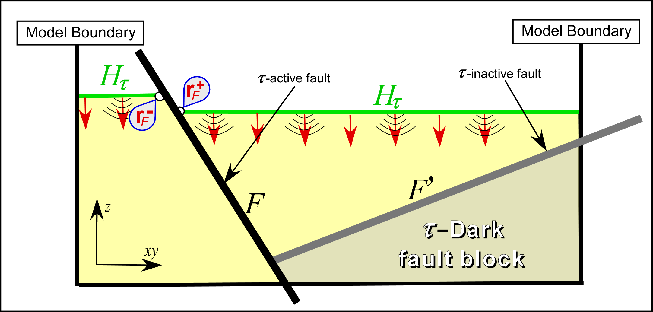
Figure 8: Vertical cross section in a structural model depicting a “$\tau$-dark” fault block (darker yellow), which cannot be illuminated by light emitted by horizon $H_{\tau}$.

6 Characterizing functions ${\{u_{\tau},v_{\tau}\}_{{\bf r}_{\tau}}}$

Solving eikonal Equation 34 provides us with the values of $t_{\tau}({\bf r}_{\tau})$ over space $G_{\tau}$. Assuming that $t_{\tau}({\bf r}_{\tau})$ is now known, this section shows how differential equations characterizing functions $\{u_{\tau},v_{\tau}\}_{{\bf r}_{\tau}}$ can be derived from the jelly paradigm and fundamental GBR principle 22.

First type boundary conditions for ${\{u_{\tau},v_{\tau}\}_{{\bf r}_{\tau}}}$ on ${H_{\tau}}$

By definition, for any point ${\bf r}_{\tau}^{o}\in H_{\tau}$:

• In the $G_{\tau}$ space, $\{u({\bf r}_{\tau}^{o}),v({\bf r}_{\tau}^{o})\}$ are the given GeoChron paleo-geographic coordinates of the particle of sediment observed today at location ${\bf r}_{\tau}^{o}$;

• In the $\overline{G}_{\tau}$ restored space, $\{u_{\tau}(\bar{\bf r}_{\tau}^{o}),v_{\tau}(\bar{\bf r}_{\tau}^{o})\}$ are unknown geographic coordinates of the particle of sediment which would have been observed at location $\bar{\bf r}_{\tau}^{o}$ on sea floor $\overline{\cal S}_{\tau}(0)$.

Obviously, taking Equations 19 into account and for any point ${\bf r}_{\tau}^{o}\in H_{\tau}$, coordinates $\{u({\bf r}_{\tau}^{o}),v({\bf r}_{\tau}^{o})\}$ and $\{u_{\tau}({\bf r}_{\tau}^{o}),v_{\tau}({\bf r}_{\tau}^{o})\}$ should be identical. As a consequence, the following first type boundary conditions, where $u({\bf r}_{\tau}^{o})$ and $v({\bf r}_{\tau}^{o})$ are known, must be honored:

$$\begin{array}[]{|c|}\hline\cr\\ \forall\ {\bf r}_{\tau}^{o}\in\{{\cal S}_{\tau}(0)\equiv H_{\tau}\}\ :\quad\left|\begin{array}[]{cccl}1)&u_{\tau}({\bf r}_{\tau}^{o})&=&u({\bf r}_{\tau}^{o})\\ \\ 2)&v_{\tau}({\bf r}_{\tau}^{o})&=&v({\bf r}_{\tau}^{o})\end{array}\right.\\ \\ \hline\cr\end{array}$$ (35)

Lovely et al., (2018) do not set the constraints specified above, which implies that functions $\{u_{\tau},v_{\tau}\}_{{\bf r}_{\tau}}$ are not synchronized with known paleo-geographic functions $\{u,v\}_{\bf r}$. As a consequence, the $uvt$-transform and $u_{\tau}v_{\tau}t_{\tau}$-transform of $H_{\tau}$ are not constrained to be identical, implying that erroneous deformations may appear on $\overline{H}_{\tau}$ obtained as $u_{\tau}v_{\tau}t_{\tau}$-transform of $H_{\tau}$. As an example, consider the (generally curvilinear) patch $H_{\tau}(u_{o},v_{o},\Delta)$ defined on $H_{\tau}$ as follows:

$${\bf r}\in H_{\tau}(u_{o},v_{o},\Delta)\quad\Longleftrightarrow\quad\left\{\begin{array}[]{ccccc}t({\bf r})=\tau\\ u_{o}\leq u({\bf r})\leq u_{o}+\Delta\\ v_{o}\leq v({\bf r})\leq v_{o}+\Delta\end{array}\right.$$ (36)

and consider also $\overline{H}_{\tau}^{\oplus}(u_{o},v_{o},\Delta)$ and $\overline{H}_{\tau}^{\ominus}(u_{o},v_{o},\Delta)$ as the restored images of $H_{\tau}(u_{o},v_{o},\Delta)$ on $\overline{H}_{\tau}$ with and without constraints 35, respectively. If constraints 35 are omitted, then $\overline{H}_{\tau}^{\oplus}(u_{o},v_{o},\Delta)$ and $\overline{H}_{\tau}^{\ominus}(u_{o},v_{o},\Delta)$ may have different areas and/or shapes, implying that the restoration process may induce deformations which are incoherent with those described by the $\{u,v,t\}_{\bf r}$ GeoChron functions provided as input.

Second type boundary conditions for ${\{u_{\tau},v_{\tau}\}_{{\bf r}_{\tau}}}$ on ${H_{\tau}}$

In the restored space $\overline{G}_{\tau}$, terrains older than $\tau$ are generally still folded and, similarly to terrains in the $G$-space, their deformation may be characterized by the “partial” strain tensor at geological-time $\tau$ denoted $\mbox{{\boldmath${\cal E}$}}({\bf r}|\tau)$. For coherency’s sake, on $H_{\tau}$ the “total” strain tensor $\mbox{{\boldmath${\cal E}$}}({\bf r})$ characterized by Equation 2.20 on page 63 of Mallet, (2014) and the “partial” strain tensor $\mbox{{\boldmath${\cal E}$}}({\bf r}|\tau)$ should be equal:

$$\mbox{{\boldmath${\cal E}$}}({\bf r}_{\tau}^{o})\ =\ \mbox{{\boldmath${\cal E}$}}({\bf r}_{\tau}^{o}|\tau)\qquad\forall\ {\bf r}_{\tau}^{o}\in H_{\tau}$$ (37)

On horizon $H_{\tau}$, as a consequence of boundary conditions 34.2b set on $t_{\tau}({\bf r}_{\tau})$, we have:

$$\mbox{\bf N}({\bf r}_{\tau}^{o})\ =\ \frac{\mathbf{grad}\,t({\bf r}_{\tau}^{o})}{||\mathbf{grad}\,t({\bf r}_{\tau}^{o})||}\ =\ \frac{\mathbf{grad}\,t_{\tau}({\bf r}_{\tau}^{o})}{||\mathbf{grad}\,t_{\tau}({\bf r}_{\tau}^{o})||}\ =\ \mbox{\bf N}_{\tau}({\bf r}_{\tau}^{o})\qquad\forall\ {\bf r}_{\tau}^{o}\in H_{\tau}$$ (38)

Therefore, barring the effects of compaction, according to GBR principle 22 and Equation 37, for all indexes $(\alpha,\beta)\in\{x,y,z\}^{2}$, Equation 8 implies:

$$\forall\ {\bf r}_{\tau}^{o}\in H_{\tau}\ :\quad\left|\begin{array}[]{llllllllll}&&\{\partial_{\alpha}u\cdot\partial_{\beta}u+\partial_{\alpha}v\cdot\partial_{\beta}v+{N^{\alpha}\cdot N^{\beta}}\}_{{\bf r}_{\tau}^{o}}\\ \\ &=&\{\partial_{\alpha}u_{\tau}\cdot\partial_{\beta}u_{\tau}+\partial_{\alpha}v_{\tau}\cdot\partial_{\beta}v_{\tau}+{N^{\alpha}\cdot N^{\beta}}\}_{{\bf r}_{\tau}^{o}}\end{array}\right.$$ (39)

$$\Longleftrightarrow\quad\forall\ {\bf r}_{\tau}^{o}\in H_{\tau}\ :\quad\left|\begin{array}[]{cllllll}&&\{\partial_{\alpha}u\cdot\partial_{\beta}u+\partial_{\alpha}v\cdot\partial_{\beta}v\}_{{\bf r}_{\tau}^{o}}\\ \\ &=&\{\partial_{\alpha}u_{\tau}\cdot\partial_{\beta}u_{\tau}+\partial_{\alpha}v_{\tau}\cdot\partial_{\beta}v_{\tau}\}_{{\bf r}_{\tau}^{o}}\end{array}\right.$$ (40)

A straightforward solution to these equations consists in constraining restoration functions $\{u_{\tau},v_{\tau}\}_{{\bf r}_{\tau}}$ as follows, where $\{u,v\}_{\bf r}$ are known:

$$\begin{array}[]{|c|}\hline\cr\\ \forall\ {\bf r}_{\tau}^{o}\in\{{\cal S}_{\tau}(0)\equiv H_{\tau}\}\ :\quad\left|\begin{array}[]{cccl}1)&\mathbf{grad}\,u_{\tau}({\bf r}_{\tau}^{o})&=&\mathbf{grad}\,u({\bf r}_{\tau}^{o})\\ \\ 2)&\mathbf{grad}\,v_{\tau}({\bf r}_{\tau}^{o})&=&\mathbf{grad}\,v({\bf r}_{\tau}^{o})\end{array}\right.\\ \\ \hline\cr\end{array}$$ (41)

This second type of boundary conditions are not implemented in Lovely et al., (2018)’s method, which may jeopardize the consistency of restored models with respect to the initial GeoChron model.

Comment

In order to maintain consistency of restoration functions $\{u_{\tau},v_{\tau},t_{\tau}\}_{{\bf r}_{\tau}}$ with input GeoChron functions $\{u,v,t\}_{{\bf r}_{\tau}}$, boundary conditions 35 and 41 must be honored as strictly as possible. If they do not conflict with these boundary conditions, other, not so strict constraints may be added and honored in a least squares sense, as for example the following “$\tau$-twin-pins” constraint.

By definition, we suggest denoting “$\tau$-twin-pins” a pair of points $({\bf r}_{\tau}^{1},{\bf r}_{\tau}^{2})$ in $G_{\tau}$ such that the structural geologist has reason to believe that their restored images $(\overline{{\bf r}}_{\tau}^{1},\overline{{\bf r}}_{\tau}^{2})$ at restoration time $\tau$ must be located on a single vertical line in $\overline{G}_{\tau}$. In order to take that constraint into account, restoration functions $\{u_{\tau},v_{\tau},t_{\tau}\}_{{\bf r}_{\tau}}$ may be computed such that, in a least squares sense:

$$\left|\begin{array}[]{ccccccccc}u_{\tau}({\bf r}_{\tau}^{1})&\simeq&u_{\tau}({\bf r}_{\tau}^{2})\\ \\ v_{\tau}({\bf r}_{\tau}^{1})&\simeq&v_{\tau}({\bf r}_{\tau}^{2})\end{array}\right.$$ (42)

By setting this type of constraint repeatedly on pairs of points located, for instance, on a line in $G_{\tau}$, it is possible to make the restored version of this line vertical in $\overline{G}_{\tau}$.

Characterizing functions ${\{u_{\tau},v_{\tau}\}_{{\bf r}_{\tau}}}$ in $G_{\tau}$

According to GeoChron theory, everywhere in studied domain $G$, terrain deformation is characterized by the gradients of geological-time function $t({\bf r})$ and paleo-geographic functions $\{u,v\}_{\bf r}$, which may be considered as deformation “records” taken into account by boundary conditions 35 and 41. As explained below, to propagate these boundary conditions over the entire $G_{\tau}$-space, the gradients of $\{u_{\tau},v_{\tau}\}_{{\bf r}_{\tau}}$ have to honor specific differential equations.

Referring to fundamental GBR principle 22, to characterize the restoration functions $\{u_{\tau},v_{\tau},t_{\tau}\}_{\bf r}$, we should simply substitute these functions to $\{u,v,t\}_{\bf r}$ in Equation 6 or Equation 7. However:

1. In $G_{\tau}$ and in accordance with GeoChron theory:

   1. “soft” constraints 6-1&2 or 7-1&2 may only be honored in a least squares sense;

   2. due to local deformations of horizons and layers induced by tectonic forces, left hand sides of constraints 6-1&2 or 7-1&2 may slightly differ from the specified value “1”.

2. On $H_{\tau}$, “hard” constraints 35 and 41 strictly specify the values of restoration functions $\{u_{\tau},v_{\tau}\}$ and their 3D gradients which, according to item 1.b above, may conflict with constraints 6-1&2 or 7-1&2.

Therefore, to resolve such a conflict, we suggest removing constraints 6-1&2 or 7-1&2 and constraining $\{u_{\tau},v_{\tau}\}_{{\bf r}_{\tau}}$ in a least squares sense as follows:

• In a minimal deformation tectonic style context:

  $$\forall\ {\bf r}_{\tau}\in G_{\tau}\ :\quad\begin{array}[]{|c|}\hline\cr\\ \begin{array}[]{cc}1)&\{\mathbf{grad}\,u_{\tau}\cdot\mathbf{grad}\,v_{\tau}\}_{{\bf r}_{\tau}}\ \simeq\ 0\\ 2)&\{\mathbf{grad}\,t_{\tau}\cdot\mathbf{grad}\,u_{\tau}\}_{{\bf r}_{\tau}}\ \simeq\ 0\\ 3)&\{\mathbf{grad}\,t_{\tau}\cdot\mathbf{grad}\,v_{\tau}\}_{{\bf r}_{\tau}}\ \simeq\ 0\end{array}\\ \\ \hline\cr\end{array}$$ (43)

• In a flexural slip tectonic style context, denoting $\mathbf{grad}_{\textsc{s}}\varphi({\bf r}_{\tau})$ the orthogonal projection of $\mathbf{grad}\,\varphi({\bf r}_{\tau})$ onto the plane tangent to the level-set ${\cal S}_{\tau}(-t_{\tau}({\bf r}_{\tau}))$ of function $t_{\tau}({\bf r}_{\tau})$ at location ${\bf r}_{\tau}$:

  $$\forall\ {\bf r}_{\tau}\in G_{\tau}\ :\quad\begin{array}[]{|c|}\hline\cr\\ \{\mathbf{grad}_{\textsc{s}}\,u_{\tau}\cdot\mathbf{grad}_{\textsc{s}}\,v_{\tau}\}_{{\bf r}_{\tau}}\ \simeq\ 0\\ \\ \hline\cr\end{array}$$ (44)

It must be noted, however, that boundary conditions 35 and 41 fully specify $\{u_{\tau},v_{\tau}\}_{{\bf r}_{\tau}}$ only on horizon $H_{\tau}$. To propagate these conditions downward throughout the whole domain $G_{\tau}$ whilst honoring constraints 43 or 44, we propose to specify that the gradients of these functions must vary as smoothly as possible in $G_{\tau}$. In practice, this may be achieved in a least squares sense thanks to the following, additional constraint:

$$\sum_{\alpha\in\{x,y,z\}}\int_{G_{\tau}}\biggl{[}||\partial_{\alpha}\mathbf{grad}\,u_{\tau}({\bf r}_{\tau})||^{2}+||\partial_{\alpha}\mathbf{grad}\,v_{\tau}({\bf r}_{\tau})||^{2}\biggr{]}\cdot d{\bf r}_{\tau}\qquad\mbox{minimum}$$ (45)

7 Accounting for faults

As shown on Figure 4, 3D geological domain $G$ may be cut by faults and GeoChron functions $\{u,v,t\}_{\bf r}$ are discontinuous across these faults. Similarly, faults induce discontinuities in GeoChron functions $\{u_{\tau},v_{\tau},t_{\tau}\}_{{\bf r}_{\tau}}$ defined on $G_{\tau}$. However, based on geological arguments presented below, values and gradients of functions $\{u_{\tau},v_{\tau},t_{\tau}\}_{{\bf r}_{\tau}}$ on either side of a fault should generally honor geometric constraints which are specific to particular types of faults.

${\tau}$-active & ${\tau}$-inactive faults

With respect to a given restoration time $\tau$, we classify faults according to the two following categories:

• A fault which intersects horizon $H_{\tau}$ is a “$\tau$-active” fault (e.g $F$ in Figure 9);

• A fault which belongs to $G_{\tau}$ and does not intersect horizon $H_{\tau}$ is a “$\tau$-inactive” fault (e.g. $F^{\prime}$ and $F^{\prime\prime}$ in Figure 9).

“$\tau$-active” or “$\tau$-inactive” status is defined relatively to restoration time $\tau$: At an older restoration time $\tau^{\prime}<\tau$, a $\tau$-inactive fault which intersects $H_{\tau^{\prime}}$ may become a $\tau^{\prime}$-active fault.

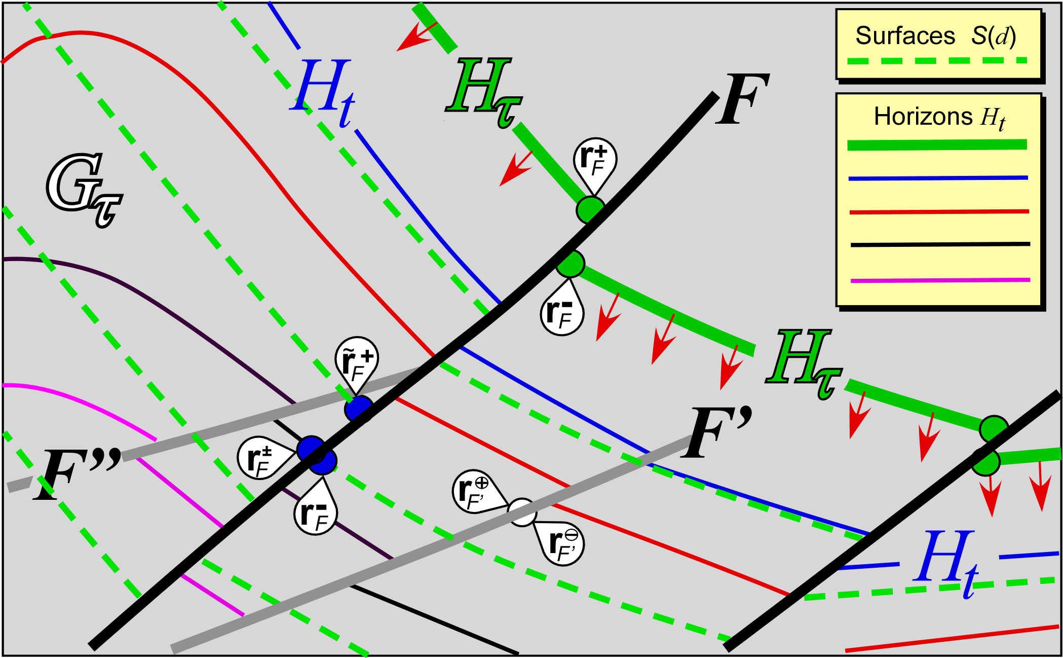
Figure 9: Vertical cross section where multicolored bold lines represent horizons $\{H_{t}:t\leq\tau\}$ and green dashed lines depict surfaces $\{{\cal S}_{\tau}(d):d\geq 0\}$ parallel to $\{H_{\tau}\equiv{\cal S}_{\tau}(0)\}$. For each pair of twin-points $({\bf r}_{\textsc{f}}^{+},{\bf r}_{\textsc{f}}^{-})$ on $H_{\tau}$, we have both $\{t_{\tau}({\bf r}_{\textsc{f}}^{+})=t_{\tau}({\bf r}_{\textsc{f}}^{-})=z_{\tau}^{o}\}$ and $\{t({\bf r}_{\textsc{f}}^{+})=t({\bf r}_{\textsc{f}}^{-})\}$. Level sets $\{{\cal S}_{\tau}(d):d\geq 0\}$ of function $t_{\tau}({\bf r}_{\tau})$ are continuous across $\tau$-inactive faults (in gray).

When horizon $H_{\tau}$ is restored, the jelly block $G_{\tau}$ underneath $H_{\tau}$ must behave as if it were only impacted by $\tau$-active faults. All other geologic objects such as horizons and $\tau$-inactive faults embedded in the jelly block are passively deformed by this restoration process. In other words, restoration functions $\{u_{\tau},v_{\tau},t_{\tau}\}_{{\bf r}_{\tau}}$ must be continuous across $\tau$-inactive faults.

However, geological domain $G_{\tau}$ is topologically discontinuous across faults of any type. In order to ensure functions $\{u_{\tau},v_{\tau},t_{\tau}\}_{{\bf r}_{\tau}}$ are ${\cal C}^{1}$-continuous across $\tau$-inactive faults, the following constraints may be set on pairs of “$\tau$-mate-points” $({\bf r}_{\textsc{f}}^{\oplus},{\bf r}_{\textsc{f}}^{\ominus})_{\tau}$ defined as collocated points lying on $F^{+}$ and $F^{-}$, respectively:

$$\begin{array}[]{|c|}\hline\cr\\ \left|\begin{array}[]{cccccccccccccccccc}1)&u_{\tau}({\bf r}_{\textsc{f}}^{\oplus})&=&u_{\tau}({\bf r}_{\textsc{f}}^{\ominus})\\ 2)&v_{\tau}({\bf r}_{\textsc{f}}^{\oplus})&=&v_{\tau}({\bf r}_{\textsc{f}}^{\ominus})\\ 3)&t_{\tau}({\bf r}_{\textsc{f}}^{\oplus})&=&t_{\tau}({\bf r}_{\textsc{f}}^{\ominus})\end{array}\right.\quad\mbox{{\boldmath${\&}$}}\quad\left|\begin{array}[]{cccccccccccccccccc}4)&\mathbf{grad}\,u_{\tau}({\bf r}_{\textsc{f}}^{\oplus})&=&\mathbf{grad}\,u_{\tau}({\bf r}_{\textsc{f}}^{\ominus})\\ 5)&\mathbf{grad}\,v_{\tau}({\bf r}_{\textsc{f}}^{\oplus})&=&\mathbf{grad}\,v_{\tau}({\bf r}_{\textsc{f}}^{\ominus})\\ 6)&\mathbf{grad}\,t_{\tau}({\bf r}_{\textsc{f}}^{\oplus})&=&\mathbf{grad}\,t_{\tau}({\bf r}_{\textsc{f}}^{\ominus})\end{array}\right.\\ \\ \forall\ ({\bf r}_{\textsc{f}}^{\oplus},{\bf r}_{\textsc{f}}^{\ominus})_{\tau}\in\ \mbox{$\tau$-inactive fault $F$}\\ \\ \hline\cr\end{array}$$ (46)

Boundary conditions for ${\{u_{\tau},v_{\tau}\}_{{\bf r}_{\tau}}}$ on ${\tau}$-active faults

When horizon $H_{\tau}$ is restored, terrains located on either side of $\tau$-active faults must slide along lines called $\tau$-fault-striae, tangent to these faults. For geological consistency, $\tau$-fault-striae must be identical to fault-striae (see Figure 5) associated with the $\{u,v\}_{\tau}$ paleo-geographic coordinates of the GeoChron model provided as input to the proposed restoration method:

$$\begin{array}[]{|c|}\hline\cr\\ \mbox{{\boldmath${\tau}$}}\mbox{-fault-striae}\ \equiv\ \mbox{fault-striae}\qquad\forall\ \tau\\ \\ \hline\cr\end{array}$$ (47)

As Lovely et al., (2018) use the standard SKUA^® algorithm to reestablish continuity of functions $\{u_{\tau},v_{\tau}\}_{{\bf r}_{\tau}}$ through faults, $\tau$-twin-points are recomputed from the geometry and topology of level-sets $\{{\cal S}(d):d\geq 0\}$ of $t_{\tau}({\bf r}_{\tau})$ in $G_{\tau}$. As a consequence, these $\tau$-twin-points may not be located on the same fault-striae as those induced by known $\{u,v,t\}_{\bf r}$ functions of the input GeoChron model (e.g., see Figure 5), which may break the consistency between input and restored model close to faults.

Similarly to GeoChron twin-points $({\bf r}_{\textsc{f}}^{+},{\bf r}_{\textsc{f}}^{-})$, $\tau$-twin-points $({\bf r}_{\textsc{f}}^{+},{\bf r}_{\textsc{f}}^{-})_{\tau}$ are characterized by the following equations:

$$\{\ ({\bf r}_{\textsc{f}}^{+},{\bf r}_{\textsc{f}}^{-})_{\tau}\mbox{ is a pair of $\tau$-twin-points }\}\quad\Longleftrightarrow\quad\left\{\begin{array}[]{ccccccc}1)&\mbox{$F$ is a $\tau$-active fault}\\ 2)&{\bf r}_{\textsc{f}}^{+}\in F^{+}\ \mbox{ \mbox{\bf\&} }\ {\bf r}_{\textsc{f}}^{-}\in F^{-}\\ \\ 3)&u_{\tau}({\bf r}_{\textsc{f}}^{-})=u_{\tau}({\bf r}_{\textsc{f}}^{+})\\ 4)&v_{\tau}({\bf r}_{\textsc{f}}^{-})=v_{\tau}({\bf r}_{\textsc{f}}^{+})\\ 5)&t_{\tau}({\bf r}_{\textsc{f}}^{-})=t_{\tau}({\bf r}_{\textsc{f}}^{+})\end{array}\right.$$ (48)

In order to restore terrains along $\tau$-active faults without creating voids or overlaps, constraints 48-3 to 48-5 must be honored all along $\tau$-active faults. Function $t_{\tau}({\bf r}_{\tau})$ is independent from $\{u_{\tau},v_{\tau}\}_{{\bf r}_{\tau}}$ and is assumed to be already known. As a consequence, $\{u_{\tau},v_{\tau}\}_{{\bf r}_{\tau}}$ simply have to honor the following constraints:

$$\begin{array}[]{|c|}\hline\cr\\ \left.\begin{array}[]{ccccccccccccc}1)&u_{\tau}({\bf r}_{\textsc{f}}^{+})&=&u_{\tau}({\bf r}_{\textsc{f}}^{-})\\ \\ 2)&v_{\tau}({\bf r}_{\textsc{f}}^{+})&=&v_{\tau}({\bf r}_{\textsc{f}}^{-})\end{array}\right\}\quad\forall\ ({\bf r}_{\textsc{f}}^{+},{\bf r}_{\textsc{f}}^{-})_{\tau}\in\mbox{ $\tau$-active fault}\\ \\ \hline\cr\end{array}$$ (49)

Why distinguish ${\tau}$-active from ${\tau}$-inactive faults?

At restoration geological-time $\tau$, any fault that isolates a fault block in $G_{\tau}$ such that pseudo light emitted by $H_{\tau}$ cannot reach it, must be considered as $\tau$-inactive in order for this fault block to be restored.

Next, considering faults that do not intersect $H_{\tau}$ as active may result in erroneous distortion of restored terrains. The top left corner of Figure 10 shows the same cross section as Figure 9 but the restoration for horizon $H_{\tau}$ is computed while considering fault $F^{\prime\prime}$, which does not intersect $H_{\tau}$, as a $\tau$-active fault.

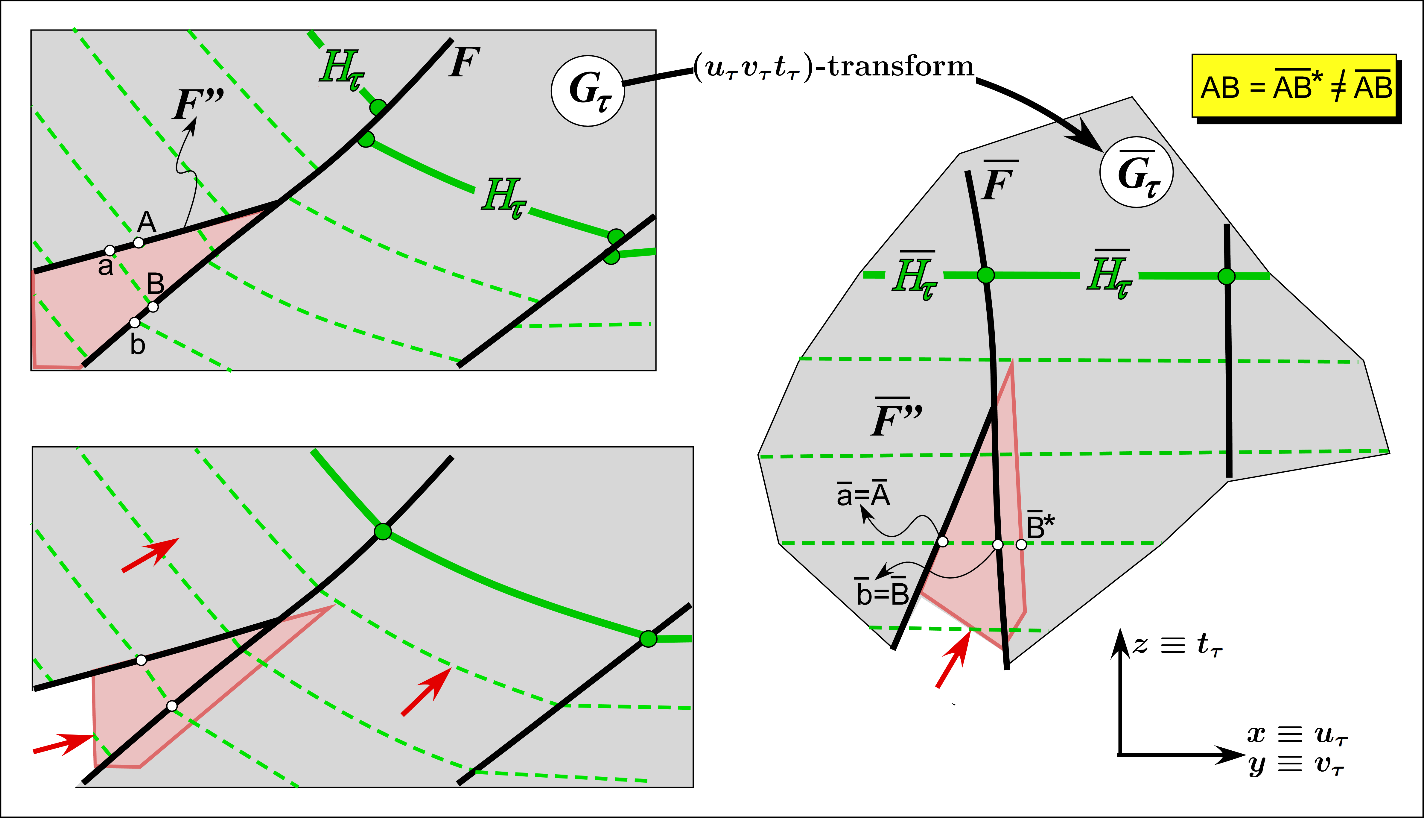
Figure 10: Vertical cross section in which fault $F^{\prime\prime}$ is erroneously considered as a $\tau$-active fault. In the restoration process induced by a $u_{\tau}v_{\tau}t_{\tau}$-transform, the distance between points A and B cannot be correctly preserved.

If fault $F^{\prime\prime}$ is considered as a $\tau$-active fault, pairs of points $(\mbox{\bf a},\mbox{\bf A})$ and $(\mbox{\bf b},\mbox{\bf B})$ shown in the top left part of Figure 10 are considered as $\tau$-twin-points. After restoration, $\tau$-twin-points are collocated, implying that $(\overline{\mbox{\bf a}}=\overline{\mbox{\bf A}})$ and $(\overline{\mbox{\bf b}}=\overline{\mbox{\bf B}})$ (right hand side of Figure 10).

As distance $(\mbox{\bf AB}=\overline{\mbox{\bf AB}^{\star}})$ differs from $(\overline{\mbox{\bf AB}}=\overline{\mbox{\bf ab}})$, in the neighborhood of faults $F$ and $F^{\prime\prime}$, a restoration performed via $u_{\tau}v_{\tau}t_{\tau}$-transform would generate incorrect variations in lengths and volumes.

To avoid these inconsistencies, distinguishing $\tau$-active and $\tau$-inactive faults is a key component of the GBR method and an improvement over the first implementation of a GeoChron restoration method by Lovely et al., (2018).

Manually activating faults

According to geological context, structural geologists may prefer some $\tau$-inactive faults to be considered as $\tau$-active, for example when a thrust fault is known to be active at a particular time even though it did not break through to the sea floor. Technically, this is possible for nearly any fault, which is then constrained with Equations 49 as any other active fault.

However, any fault bordering a $\tau$-dark fault block (e.g. Figure 8) must be handled as $\tau$-inactive, otherwise functions $\{u_{\tau},v_{\tau},t_{\tau}\}_{{\bf r}_{\tau}}$ would be undetermined inside this $\tau$-dark fault block which, as a consequence, could not be restored.

8 Taking compaction into account

Compaction is defined as pore space reduction in sediments due to increased load during deposition. As this process changes the geometry of geological layers as their depths increase, restoration workflows frequently handle compaction as an option.

As we have done so far, assume that an initial version of restoration functions $\{u_{\tau},v_{\tau},t_{\tau}\}_{{\bf r}_{\tau}}$ has been obtained without taking compaction into account. In other words, the compacted thicknesses of layers in studied domain $G_{\tau}$, as observed today, have been approximately preserved in restored domain $\overline{G}_{\tau}$. In effect, restoration uplifts and unloads terrains, which should induce decompaction resulting in increased layer thicknesses in the restored domain.

In this section we show how $\{u_{\tau},v_{\tau},t_{\tau}\}_{{\bf r}_{\tau}}$ can be replaced by new restoration functions in such a way that the new $u_{\tau}v_{\tau}t_{\tau}$-transform $\overline{G}_{\tau}$ of $G_{\tau}$ so obtained restores the terrains and induces thickness variations as a consequence of decompaction, which should be the exact inverse of the compaction that occurred between geological-time $\tau$ and the present geological-time.

Athy’s law

As the concept of decompaction may be easier to grasp in the restored space, we refer to Figure 7-D which shows the subsurface restored at geological-time $\tau$. Let $\overline{V}(\overline{{\bf r}}_{\tau})$ be an infinitely small volume of sediment centered on point $\overline{{\bf r}}_{\tau}\in\overline{G}_{\tau}$ underneath the sea floor $\{\overline{\cal S}_{\tau}(0)\equiv\overline{H}_{\tau}\}$.

Laboratory experiments on rock samples show that, during burial when sediments contained in $\overline{V}(\overline{{\bf r}}_{\tau})$ compact under their own weight, their porosity $\overline{\Psi}(\overline{{\bf r}}_{\tau})$ exponentially decreases according to Athy’s law (Athy,, 1930):

$$\overline{\Psi}(\overline{{\bf r}}_{\tau})\ \simeq\ \overline{\Psi}_{o}(\overline{{\bf r}}_{\tau})\cdot exp\biggl{\{}-\overline{\kappa}(\overline{{\bf r}}_{\tau})\cdot\delta(\overline{{\bf r}}_{\tau})\biggr{\}}\qquad\forall\ \overline{{\bf r}}_{\tau}\in\overline{G}_{\tau}$$ (50)

In this equation, $\delta(\overline{{\bf r}}_{\tau})$ is the absolute distance, or depth, from point $\overline{{\bf r}}_{\tau}\in\overline{G}_{\tau}$ to sea floor $\overline{\cal S}_{\tau}(0)$ measured at geological-time $\tau$ whilst $\overline{\Psi}_{o}(\overline{{\bf r}}_{\tau})<1$ and $\overline{\kappa}(\overline{{\bf r}}_{\tau})>0$ are known non-negative coefficients which only depend on rock type at location $\overline{{\bf r}}_{\tau}$. As an example, assuming that $\delta(\overline{{\bf r}}_{\tau})$ is expressed in meters, the following average coefficients for sedimentary terrains observed in southern Morocco have been reported (Labbassi,, 1999):

$Rock\ type$	$\overline{\Psi}_{o}$	$\overline{\kappa}$
Siltstone	0.62	0.57$\times 10^{-3}$
Clay	0.71	0.77$\times 10^{-3}$
Sandstone	0.35	0.60$\times 10^{-3}$
Carbonates	0.46	0.23$\times 10^{-3}$
Dolomites	0.21	0.61$\times 10^{-3}$

Keeping in mind that, in the restored $\overline{G}_{\tau}$-space, $\{-{t}_{\tau}(\overline{{\bf r}}_{\tau})\}$ measures the vertical distance from $\overline{{\bf r}}_{\tau}$ to sea floor $\overline{S}_{\tau}(0)$, in Equation 50, depth function $\delta(\overline{{\bf r}}_{\tau})$ can be expressed as follows:

$$\delta(\overline{{\bf r}}_{\tau})\ =\ -{t}_{\tau}(\overline{{\bf r}}_{\tau})\qquad\forall\ \overline{{\bf r}}_{\tau}\in\overline{G}_{\tau}$$ (51)

As a consequence, in the context of our GBR method, Athy’s law may straightforwardly be reformulated as:

$$\overline{\Psi}(\overline{{\bf r}}_{\tau})\ \simeq\ \overline{\Psi}_{o}(\overline{{\bf r}}_{\tau})\cdot exp\biggl{\{}\overline{\kappa}(\overline{{\bf r}}_{\tau})\cdot{t}_{\tau}(\overline{{\bf r}}_{\tau})\biggr{\}}\qquad\forall\ \overline{{\bf r}}_{\tau}\in\overline{G}_{\tau}$$ (52)

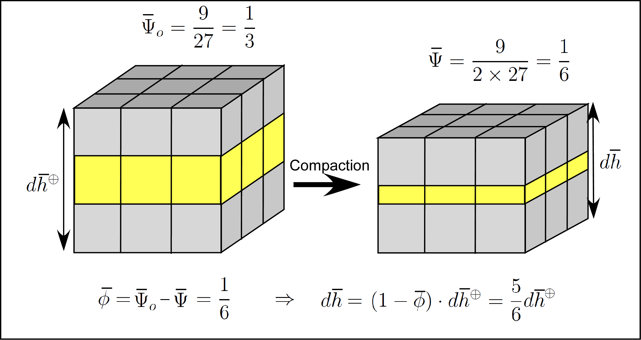
Figure 11: Porosity versus compaction: Infinitely small column of sediment where, under vertical compaction, the vertical dimension of pores represented in yellow is halved. As a result, $(d\bar{h}^{\oplus}=3)$ becomes $(d\bar{h}=2.5)$. Note that yellow and gray cells may be randomly swapped in the vertical direction without altering these results.

Decompaction in ${\overline{G}_{\tau}}$

Elasto-plastic mechanical frameworks developed to model compaction rely on a number of input parameters which may be difficult for a geologist or geomodeler to assess and require solving a complex system of equations (Schneider et al.,, 1996). Isostasic approaches are simpler to parameterize and still provide useful information on basin evolution (Durand-Riard et al.,, 2011). Therefore, we will consider compaction as a mainly one-dimensional, vertical process induced by gravity which mainly occurs in the early stages of sediment burial when horizons are still roughly horizontal surfaces close to the sea floor. At any point $\overline{{\bf r}}_{\tau}\in\overline{G}_{\tau}$ within a layer, the decompacted thickness $d\bar{h}^{\oplus}(\overline{{\bf r}}_{\tau})$ of a vertical probe consisting of an infinitely short column of sediment roughly orthogonal to the restored horizon passing through $\overline{{\bf r}}_{\tau}$ is linked to the thickness $d\bar{h}(\overline{{\bf r}}_{\tau})$ of the shorter, compacted vertical column by the following relationship:

$$\forall\ \overline{{\bf r}}_{\tau}\in\overline{G}_{\tau}\ :\quad\left|\begin{array}[]{c}d\bar{h}^{\oplus}(\overline{{\bf r}}_{\tau})\ =\ \displaystyle\frac{1}{1-\overline{\phi}_{\tau}(\overline{{\bf r}}_{\tau})}\cdot d\bar{h}(\overline{{\bf r}}_{\tau})\\ \\ \mbox{with : }\overline{\phi}_{\tau}(\overline{{\bf r}}_{\tau})=\overline{\Psi}_{o}(\overline{{\bf r}}_{\tau})-\overline{\Psi}(\overline{{\bf r}}_{\tau})\in[0,1[\end{array}\right.$$ (53)

In this equation, $\overline{\phi}(\overline{{\bf r}}_{\tau})$ denotes the “compaction coefficient” which characterizes vertical shortening of the probe at restored location $\overline{{\bf r}}_{\tau}\in\overline{G}_{\tau}$. As an example, Figure 11 shows the same infinitely short vertical column of sediment where average porosity is equal to $(\overline{\Psi}_{o}=1/3)$ before compaction and $(\overline{\Psi}=1/6)$ after compaction. The compaction coefficient $(\overline{\Psi}_{o}-\overline{\Psi})$ is then equal to $(\overline{\phi}=1/6)$ and column shortening $(1-\overline{\phi})$ is $(5/6)$.

Taking present day compaction in ${\overline{G}_{\tau}}$ into account

So far, in the context of our GBR method, the restored $\overline{G}_{\tau}$-space has been built assuming that there is no compaction. As a consequence, $\overline{G}_{\tau}$ we obtained so far is incorrect because it has undergone compaction characterized by present day porosity $\overline{\Psi}_{p}(\overline{{\bf r}}_{\tau})$.

Let $\bar{\phi}_{\tau}^{\ominus}(\overline{{\bf r}}_{\tau})$ and $\bar{\phi}_{\tau}^{\oplus}(\overline{{\bf r}}_{\tau})$ be the pair of given functions defined by:

$$\forall\ \overline{{\bf r}}_{\tau}\in\overline{G}_{\tau}\ :\quad\left|\begin{array}[]{llllllllllll}\bar{\phi}_{\tau}^{\ominus}(\overline{{\bf r}}_{\tau})&=&\bar{\Psi}_{o}(\overline{{\bf r}}_{\tau})-\overline{\Psi}_{p}(\overline{{\bf r}}_{\tau})\\ \\ \bar{\phi}_{\tau}^{\oplus}(\overline{{\bf r}}_{\tau})&=&\bar{\Psi}_{o}(\overline{{\bf r}}_{\tau})-\overline{\Psi}(\overline{{\bf r}}_{\tau})\end{array}\right.$$ (54)

where, for coherency with Athy’s law, present day porosity $\overline{\Psi}_{p}(\overline{{\bf r}}_{\tau})$ is assumed to honor the following constraint:

$$\overline{\Psi}_{\bf p}(\overline{{\bf r}}_{\tau})\ \leq\ \overline{\Psi}(\overline{{\bf r}}_{\tau})\qquad\forall\ \overline{{\bf r}}_{\tau}\in\overline{G}_{\tau}$$ (55)

Note that such a constraint implies that $\phi_{\tau}^{\oplus}({{\bf r}}_{\tau})\leq\phi_{\tau}^{\ominus}({{\bf r}}_{\tau})$.

Considering once again the vertical probe introduced above in restored space $\overline{G}_{\tau}$ and using equation 53 twice in a forward then backward way, to take compaction into account, we propose the following two steps:

1. First, to cancel out the compaction characterized by given, present day porosity $\overline{\Psi}_{p}(\overline{{\bf r}}_{\tau})$, a “total”, vertical decompaction is applied by updating $d\bar{h}(\overline{{\bf r}}_{\tau})$ as follows:

   $$d\bar{h}_{o}(\overline{{\bf r}}_{\tau})\ =\ \displaystyle\frac{1}{1-\bar{\phi}_{\tau}^{\ominus}(\overline{{\bf r}}_{\tau})}\cdot d\bar{h}(\overline{{\bf r}}_{\tau})$$ (56)

   After this first operation, probe porosity is equal to $\overline{\Psi}_{o}(\overline{{\bf r}}_{\tau})$.

2. Next, a “partial” recompaction is applied as a function of the actual porosity $\overline{\Psi}(\overline{{\bf r}}_{\tau})$ approximated by Athy’s law 52 at geological-time $\tau$:

   $$d\bar{h}^{\oplus}(\overline{{\bf r}}_{\tau})\ =\ \displaystyle\{1-\bar{\phi}_{\tau}^{\oplus}(\overline{{\bf r}}_{\tau})\}\cdot d\bar{h}_{o}(\overline{{\bf r}}_{\tau})$$ (57)

   After this second operation, probe porosity is equal to $\overline{\Psi}(\overline{{\bf r}}_{\tau})$.

Therefore, to take present-day compaction into account, Equation 53 must be replaced by:

$$d\bar{h}^{\oplus}(\overline{{\bf r}}_{\tau})\ =\ \displaystyle\frac{1-\bar{\phi}_{\tau}^{\oplus}(\overline{{\bf r}}_{\tau})}{1-\bar{\phi}_{\tau}^{\ominus}(\overline{{\bf r}}_{\tau})}\cdot d\bar{h}(\overline{{\bf r}}_{\tau})\qquad\forall\ \overline{{\bf r}}_{\tau}\in\overline{G}_{\tau}$$ (58)

GBR approach to decompaction in ${\overline{G}_{\tau}}$

In the restored $\overline{G}_{\tau}$-space, ${t}_{\tau}(\overline{{\bf r}}_{\tau})$ may be interpreted as an arc-length abscissa ${s}(\overline{{\bf r}}_{\tau})$ along the vertical straight line passing through $\overline{{\bf r}}_{\tau}$ oriented in the same direction as the vertical unit frame vector $\{\overline{{\bf r}}_{t_{\tau}}={\bf r}_{z}\}$. Therefore, in the $\overline{G}_{\tau}$-space,

$$d{t}_{\tau}(\overline{{\bf r}}_{\tau})\ =\ ds(\overline{{\bf r}}_{\tau})\ =\ d\overline{h}(\overline{{\bf r}}_{\tau})$$ (59)

is the height of an infinitely short vertical column of restored sediment located at point $\overline{{\bf r}}_{\tau}\in\overline{G}_{\tau}$, subject to present-day compaction. As a consequence, to take compaction into account in the restored $\overline{G}_{\tau}$-space, according to Equations 58 and 59, function ${t}_{\tau}(\overline{{\bf r}}_{\tau})$ must be replaced by a “decompacted” function ${t}_{\tau}^{\oplus}(\overline{{\bf r}}_{\tau})$ such that:

$$\frac{d{t}_{\tau}^{\oplus}}{d{t}_{\tau}}\bigg{|}_{\overline{{\bf r}}_{\tau}}\ =\ \displaystyle\frac{d\bar{h}^{\oplus}(\overline{{\bf r}}_{\tau})}{d\bar{h}(\overline{{\bf r}}_{\tau})}\ =\ \displaystyle\frac{1-\bar{\phi}_{\tau}^{\oplus}(\overline{{\bf r}}_{\tau})}{1-\bar{\phi}_{\tau}^{\ominus}(\overline{{\bf r}}_{\tau})}$$ (60)

Assuming that $\{\overline{{\bf r}}_{t_{\tau}}={\bf r}_{z}\}$ is the unit vertical frame vector of the $\overline{G}_{\tau}$-space, it is well known that

$$\mathbf{grad}\,{t}_{\tau}^{\oplus}(\overline{{\bf r}}_{\tau})\cdot\ \overline{{\bf r}}_{t_{\tau}}\ =\ \frac{d{t}_{\tau}^{\oplus}(\overline{{\bf r}}_{\tau}+{s}\cdot\overline{{\bf r}}_{t_{\tau}})}{d{s}}\bigg{|}_{s=0}\ =\ \frac{d{t}_{\tau}^{\oplus}}{d{t}_{\tau}}\bigg{|}_{\overline{{\bf r}}_{\tau}}$$ (61)

from which we can conclude that the current altitude ${t}_{\tau}(\overline{{\bf r}}_{\tau})$ of point $\overline{{\bf r}}_{\tau}\in\overline{G}_{\tau}$ should be transformed into a decompacted altitude ${t}_{\tau}^{\oplus}(\overline{{\bf r}}_{\tau})$ honoring the following differential equation:

$$\begin{array}[]{|c|}\hline\cr\\ \quad\displaystyle\mathbf{grad}\,{t}_{\tau}^{\oplus}(\overline{{\bf r}}_{\tau})\cdot\overline{{\bf r}}_{{t}_{\tau}}\ =\ \frac{1-{\phi}_{\tau}^{\oplus}(\overline{{\bf r}}_{\tau})}{1-{\phi}_{\tau}^{\ominus}(\overline{{\bf r}}_{\tau})}\qquad\forall\ \overline{{\bf r}}_{\tau}\in\overline{G}_{\tau}\\ \\ \mbox{with : }\quad\bar{\phi}_{\tau}^{\oplus}(\overline{{\bf r}}_{\tau})=\overline{\Psi}_{o}(\overline{{\bf r}}_{\tau})-\overline{\Psi}(\overline{{\bf r}}_{\tau})\quad\&\quad\bar{\phi}_{\tau}^{\ominus}(\overline{{\bf r}}_{\tau})=\overline{\Psi}_{o}(\overline{{\bf r}}_{\tau})-\overline{\Psi}_{p}(\overline{{\bf r}}_{\tau})\\ \\ \hline\cr\end{array}$$ (62)

Due to the vertical nature of compaction, on $\{\overline{\cal S}(0)\equiv\overline{H}_{\tau}\}$, function ${t}_{\tau}^{\oplus}(\overline{{\bf r}}_{\tau})$ should vanish and its gradient should be vertical. In other words, in addition to constraint 62, function ${t}_{\tau}^{\oplus}(\overline{{\bf r}}_{\tau})$ must also honor the following boundary conditions where $\overline{{\bf r}}_{u_{\tau}}$ and $\overline{{\bf r}}_{v_{\tau}}$ are the unit horizontal frame vectors of the $\overline{G}_{\tau}$-space:

$$\begin{array}[]{|c|}\hline\cr\\ \quad\forall\ \overline{{\bf r}}_{\tau}^{o}\in\{\overline{\cal S}_{\tau}(0)\equiv\overline{H}_{\tau}\}\ :\quad\left|\begin{array}[]{cc}1)&t_{\tau}^{\oplus}(\bar{\bf r}_{\tau}^{o})=\ 0\\ \\ 2)&\mathbf{grad}\,{t}_{\tau}^{\oplus}(\overline{{\bf r}}_{\tau}^{o})\cdot\overline{{\bf r}}_{\bar{u}_{\tau}}\ =\ 0\\ 3)&\mathbf{grad}\,{t}_{\tau}^{\oplus}(\overline{{\bf r}}_{\tau}^{o})\cdot\overline{{\bf r}}_{\bar{v}_{\tau}}\ =\ 0\end{array}\right.\\ \\ \hline\cr\end{array}$$ (63)

As compaction is a continuous process, ${t}_{\tau}^{\oplus}(\overline{{\bf r}}_{\tau})$ must be ${\cal C}^{o}$-continuous across all faults affecting $\overline{G}_{\tau}$. As a consequence, in addition to constraints 62 and 63, for any fault $\overline{F}$ in $\overline{G}_{\tau}$, function ${t}_{\tau}^{\oplus}(\overline{{\bf r}}_{\tau})$ must also honor the following boundary conditions where $(\overline{{\bf r}}_{\textsc{f}}^{\oplus},\overline{{\bf r}}_{\textsc{f}}^{\ominus})_{\tau}$ are pairs of “$\tau$-mate-points”defined as collocated points lying on the positive face $\overline{F}^{+}$ and negative face $\overline{F}^{-}$ of $\overline{F}$ at geological-time $\tau$:

$$\begin{array}[]{|c|}\hline\cr\\ \begin{array}[]{c}{t}_{\tau}(\overline{{\bf r}}_{\textsc{f}}^{\oplus})\ =\ {t}_{\tau}(\overline{{\bf r}}_{\textsc{f}}^{\ominus})\\ \\ \forall\ \overline{F}\in\overline{G}_{\tau}\quad\&\quad\forall\ (\overline{{\bf r}}_{\textsc{f}}^{\oplus},\overline{{\bf r}}_{\textsc{f}}^{\ominus})_{\tau}\in\ \overline{F}\end{array}\\ \\ \hline\cr\end{array}$$ (64)

Using an appropriate numerical method, ${t}_{\tau}^{\oplus}({\bf r}_{\tau})$ must be computed in $\overline{G}_{\tau}$ whilst ensuring that differential equation 62 and boundary conditions 63 and 64 are honored. To ensure smoothness and uniqueness of ${t}_{\tau}^{\oplus}({\bf r}_{\tau})$, the following constraint may also be added:

$$\sum_{(a,b)\in\{u_{\tau},v_{\tau},t_{\tau}\}^{2}}\int_{\overline{G}_{\tau}}\biggl{\{}\partial_{a}\partial_{b}\,{t}_{\tau}^{\oplus}(\overline{{\bf r}}_{\tau})\biggr{\}}^{2}\cdot d\overline{{\bf r}}_{\tau}\qquad\mbox{minimum}$$ (65)

As a conclusion, to take compaction into account, the following GBR approach may be used:

1. Compute a numerical approximation of ${t}_{\tau}^{\oplus}(\overline{{\bf r}}_{\tau})$ in $\overline{G}_{\tau}$ and use the reverse $u_{\tau}v_{\tau}t_{\tau}$-transform to update ${t}_{\tau}({{\bf r}}_{\tau})$ in ${G}_{\tau}$:

   $${t}_{\tau}({{\bf r}}_{\tau})\longleftarrow\ {t}_{\tau}^{\oplus}(\overline{{\bf r}}_{\tau})\qquad\forall\ {{\bf r}}_{\tau}\in G_{\tau};$$ (66)

2. Recompute numerical approximations of restoration functions $u_{\tau}({\bf r}_{\tau})$ and $v_{\tau}({\bf r}_{\tau})$ in $G_{\tau}$ to prevent voids and overlaps in the restored space, as, according to Equations 43 and 44, $u_{\tau}({\bf r}_{\tau})$ and $v_{\tau}({\bf r}_{\tau})$ depend on $t_{\tau}({\bf r}_{\tau})$;

3. Build the “decompacted” restored space $\overline{G}_{\tau}$ as the new, direct $u_{\tau}v_{\tau}t_{\tau}$-transform of geological space $G_{\tau}$ observed today.

This approach to decompaction is fully derived from the GBR framework described in this paper and differs from the sequential decompaction following Athy’s law along IPG-lines applied by Lovely et al., (2018).

9 Constraints summary

Among all the equations presented so far, Equations 34-1, 35, 41 and 49 are the most critical.

First and above all, honoring constraint 34-1 as closely as possible is the very heart of the proposed GBR method. Due to local deformations of horizons, this equation may generally be honored only in a least squares sense. However, if $||\mathbf{grad}\,t_{\tau}||_{\bf r}$ deviates too much from 1, then, during the restoration process, layer thicknesses will not be preserved, which may induce undesirable volume variations; and due to constraints 43 or 44 based on $t_{\tau}({\bf r}_{\tau})$, restoration functions $\{u_{\tau},v_{\tau}\}_{{\bf r}_{\tau}}$ will be incorrect.

Next, constraints 49 are of paramount importance because, during restoration of horizon $H_{\tau}$, they prevent gaps and overlaps from appearing in $\overline{G}_{\tau}$ along faults.

Finally, constraints 35 and 41 are also extremely important because they preserve coherency of restored surface $\overline{H}_{\tau}$ viewed either as the $u_{\tau}v_{\tau}t_{\tau}$-transform or the regular GeoChron $uvt$-transform of $H_{\tau}$. Without constraints 35, the GBR method would not be consistent with the input GeoChron model.

Comment: Volume preservation

Barring the effects of compaction, let us consider, in the $G_{\tau}$-space, a pseudo-layer $L(d,\varepsilon)$ with infinitely small thickness $\varepsilon$ bounded by pseudo-horizons ${\cal S}(d)$ and ${\cal S}(d-\varepsilon)$. Because of eikonal constraint 34, in the $\overline{G}_{\tau}$-space, restored layer $\overline{L}(d,\varepsilon)$ holds as closely as possible the same thickness $\varepsilon$ as $L(d,\varepsilon)$.

Consider now, in the $G_{\tau}$-space, an infinitely small compact patch $\Delta{\cal S}(d)$ drawn on ${\cal S}(d)$ and let $\Delta{\cal S}(d-\varepsilon)$ be the projection of this patch onto ${\cal S}(d-\varepsilon)$ along lines with constant $\{u_{\tau},v_{\tau}\}$ coordinates passing through ${\cal S}(d)$. Let $\Delta V(d,\varepsilon)$ be the infinitely small volume bounded by $\Delta{\cal S}(d)$, $\Delta{\cal S}(d-\varepsilon)$ and the field of lines defined above. During restoration, depending on the structural style, two cases have to be considered:

• if the structural style is flexural slip, by definition, areas and angles on surfaces ${\cal S}(d)$ and ${\cal S}(d-\varepsilon)$ are preserved;

• if the structural style is minimal deformation, by definition, deformations of areas and angles on surfaces ${\cal S}(d)$ and ${\cal S}(d-\varepsilon)$ are minimized, as much as possible.

Therefore, omitting compaction, as in both cases thickness $\varepsilon$ is preserved as much as possible, volumes of $\Delta V(d,\varepsilon)$ and its restored version $\overline{\Delta}V(d,\varepsilon)$ are as identical as possible.

10 Numerically approximating ${\{u_{\tau},v_{\tau},t_{\tau}\}}$

From a theoretical standpoint, restoration functions $\{u_{\tau},v_{\tau},t_{\tau}\}_{{\bf r}_{\tau}}$ are solutions to a wide system of partial differential equations presented so far in this paper. However, from a practical perspective, these equations are often non linear and coupled, which makes them difficult to solve. Many general numerical techniques known in the art could be employed but, as we show in the following, the geological nature of our problem makes it possible for us to replace these complex differential equations by surrogates which are easier to solve.

About the eikonal equation

As pointed out in the previous section, computing a function $t_{\tau}({\bf r}_{\tau})$ which honors eikonal Equation 34 is the corner-stone of our proposed GBR method but Equation 34-1, recalled below, is not linear:

$$||\mathbf{grad}\,t_{\tau}({\bf r}_{\tau})||=1\qquad\forall\ {\bf r}_{\tau}\in G_{\tau}$$ (67)

Through Equations 43 or 44, any excessive violation of this constraint also impacts functions $\{u_{\tau},v_{\tau}\}_{{\bf r}_{\tau}}$ and the resulting restoration is then inevitably incorrect.

Based on the test example shown in Figure 12, where horizon $H_{\tau}$ to restore is the central sigmoid surface, results obtained with two different numerical techniques are compared and shown on Figure 13. This seemingly simple test is actually highly significant because it shows local variations in curvature which make eikonal Equation 67 difficult to approximate numerically.

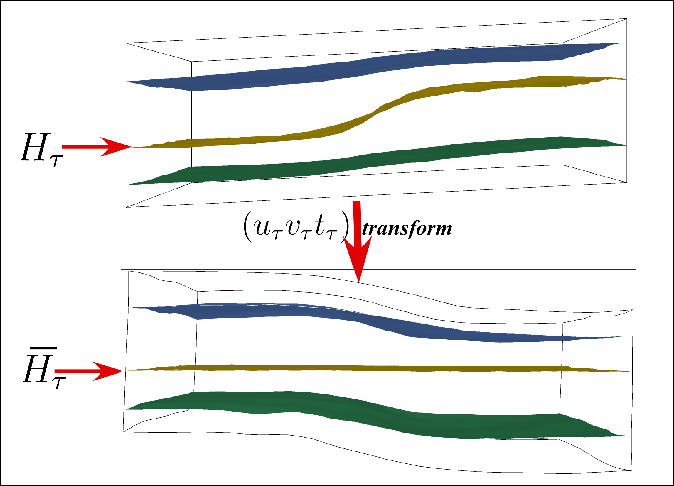
Figure 12: Test example: GBR of a “ramp” structure. Restored horizon $H_{\tau}$ is the central, sigmoid surface. Note that main curvature of $H_{\tau}$ locally varies and the associated curvature center moves from one side to the opposite side of $H_{\tau}$.

Computing ${t_{\tau}({\bf r}_{\tau})}$: Surrogate (weak) eikonal equations

We have stated before that:

$$\mathbf{grad}\,t_{\tau}({\bf r}_{\tau}^{o})\ =\ \mbox{\bf N}({\bf r}_{\tau}^{o})\ =\ \frac{\mathbf{grad}\,t({\bf r}_{\tau}^{o})}{||\mathbf{grad}\,t({\bf r}_{\tau}^{o})||}\qquad\forall\ {\bf r}_{\tau}^{o}\in H_{\tau}$$ (68)

which means that eikonal Equation 34 is approximately equivalent to the following system called “surrogate-eikonal” equation:

$$\left|\begin{array}[]{cccc}1)&\displaystyle\sum_{\alpha\in\{x,y,z\}}\int_{G_{\tau}}||\partial_{\alpha}\,\mathbf{grad}\,t_{\tau}({\bf r}_{\tau})||^{2}\cdot d{\bf r}_{\tau}\qquad\mbox{minimum}\\ \\ 2)&\mbox{subject to : \ }\left\{\begin{array}[]{cclllll}a)&t_{\tau}({\bf r}_{\tau}^{o})=0\\ \\ b)&\displaystyle\mathbf{grad}\,t_{\tau}({\bf r}_{\tau}^{o})=\mbox{\bf N}({\bf r}_{\tau}^{o})\end{array}\right\}\quad\forall\ {\bf r}_{\tau}^{o}\in H_{\tau}\end{array}\noindent\right.$$ (69)

Eikonal Equations 34-2 are strictly honored on $H_{\tau}$ and Equation 69-1 is assumed to smoothly propagate $\mathbf{grad}\,t_{\tau}({\bf r})$ in such a way that, everywhere inside $G_{\tau}$ and similarly to Equation 34-1, $\mathbf{grad}\,t_{\tau}({\bf r}_{\tau})$ roughly remains a unit vector field. In practice, according to techniques known in the art, Equation 69-1 may be linearly approximated so that each Equation 69 is linear and, therefore, easier to solve than “true” eikonal equation  34.

As mentioned above, at any point ${\bf r}_{\tau}\in G_{\tau}$, Equation 69-1 should ensure that $||\mathbf{grad}\,t_{\tau}({\bf r}_{\tau})||$ is equal to its unit starting value on $H_{\tau}$. Unfortunately, away from $H_{\tau}$, numerical drift usually makes $||\mathbf{grad}\,t_{\tau}({\bf r}_{\tau})||$ deviate from target value 1. As a consequence, eikonal constraint 34-1 is generally not perfectly honored away from $\{{\cal S}_{\tau}(0)\equiv H_{\tau}\}$, which implies that, after restoration, distortions inevitably appear in the vertical direction of the $\overline{G}_{\tau}$-space.

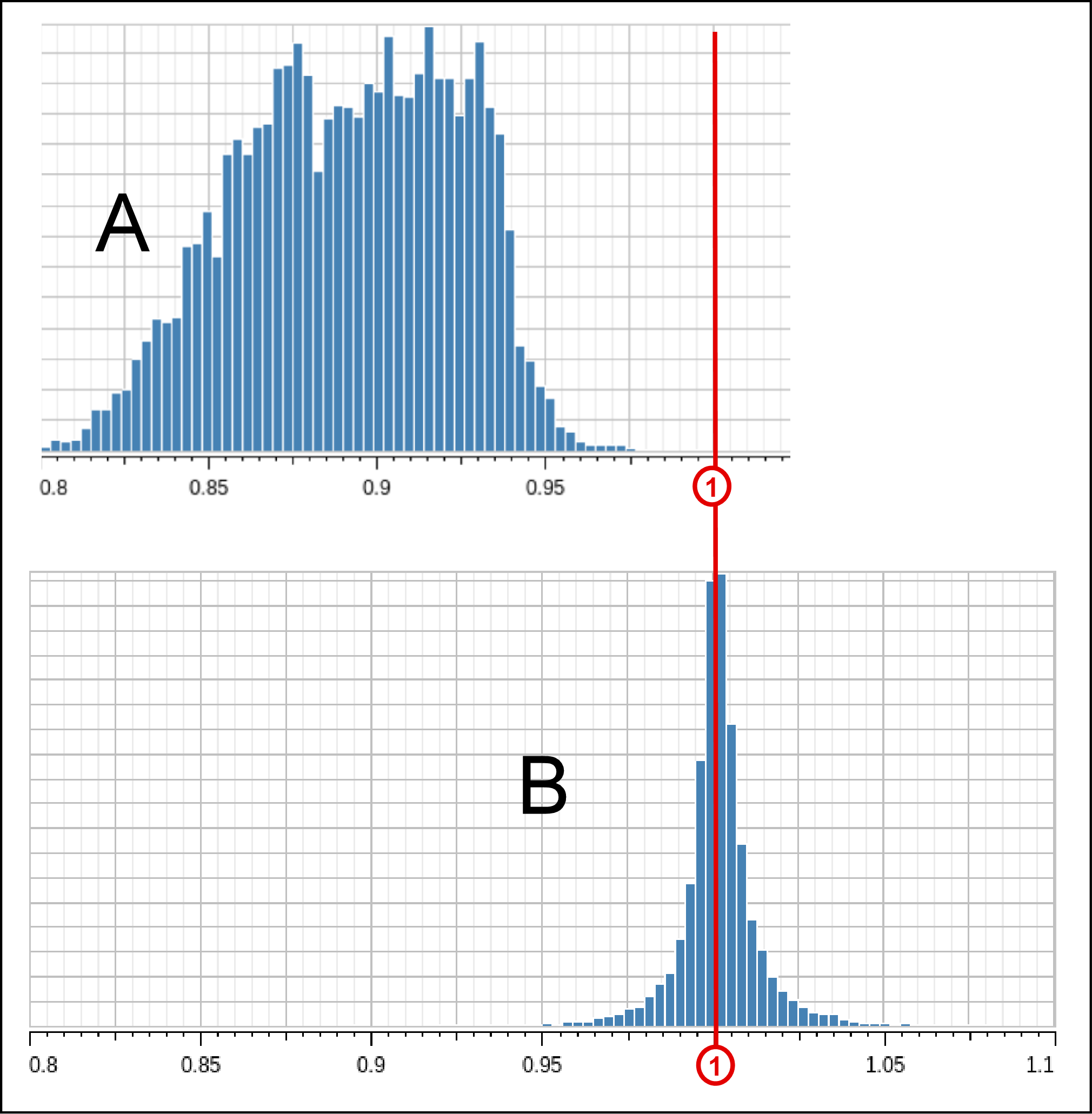
Figure 13: Test example showing histograms of $||\mathbf{grad}\,t_{\tau}({\bf r}_{\tau})||$ in the studied domain corresponding to Figure 12. Depending on the method used to compute $t_{\tau}({\bf r}_{\tau})$, the resulting magnitude of $||\mathbf{grad}\,t_{\tau}({\bf r}_{\tau})||$ may severely deviate from value “1” required by eikonal Equation 34-1. Note that, for clarity’s sake, the vertical axis of histogram (B) has been shrunk by a factor of 3.

On Figure 13-A, the histogram of $||\mathbf{grad}\,t_{\tau}({\bf r}_{\tau})||$ so obtained in $G_{\tau}$ with surrogate eikonal Equations 69 applied to our test example clearly shows that eikonal Equation 34-1 is not honored correctly. First, $||\mathbf{grad}\,t_{\tau}({\bf r}_{\tau})||$ is never equal to 1. Next, the median value is about 0.89, which represents an error of 11 %. Finally, standard deviation is 0.032 and the spread between 25^th and 75^th percentiles is 0.051.

We can conclude from these figures that approximating eikonal Equation 34-1 by Equations 69 does not give precise enough results.

Computing ${t_{\tau}({\bf r}_{\tau})}$: A precise incremental solution

Generally, even though eikonal Equation 34-1 is not perfectly honored, function $t_{\tau}({\bf r}_{\tau})$ generated by Equations 69 may be considered as an approximation of the actual solution. In other words, assuming that $t_{\tau}^{\star}({\bf r})$ is a first approximation of $t_{\tau}({\bf r}_{\tau})$, there is an unknown function $\varepsilon_{\tau}({\bf r}_{\tau})$ which may be used as follows to compute, in a post-processing step, an improved version of $t_{\tau}({\bf r}_{\tau})$:

$$t_{\tau}({\bf r}_{\tau})\ =\ t_{\tau}^{\star}({\bf r}_{\tau})+\varepsilon_{\tau}({\bf r}_{\tau})$$ (70)

with

$$\varepsilon_{\tau}({\bf r}_{\tau}^{o})\ =\ -t_{\tau}^{\star}({\bf r}_{\tau}^{o})\qquad\ \forall\ {\bf r}_{\tau}^{o}\in H_{\tau}$$ (71)

and where $t_{\tau}^{\star}({\bf r}_{\tau})$ is assumed to be precise enough to honor:

$$||\mathbf{grad}\,\varepsilon_{\tau}({\bf r}_{\tau})||\ \ll\ ||\mathbf{grad}\,t_{\tau}^{\star}({\bf r}_{\tau})||\ \simeq\ 1\qquad\ \forall\ {\bf r}_{\tau}\in G_{\tau}$$ (72)

Through faults, $\varepsilon_{\tau}({\bf r}_{\tau})$ is assumed to behave in a similar way to function $t_{\tau}({\bf r}_{\tau})$. In other words, referring to constraints 46, for any pair of $\tau$-mate-points $({\bf r}_{\textsc{f}}^{\oplus},{\bf r}_{\textsc{f}}^{\ominus})$ located on a $\tau$-inactive fault $F$, function $\varepsilon_{\tau}({\bf r}_{\tau})$ and its gradient must honor the following equations:

$$\left.\begin{array}[]{cccccccccccccccccc}1)&\varepsilon_{\tau}({\bf r}_{\textsc{f}}^{\oplus})-\varepsilon_{\tau}({\bf r}_{\textsc{f}}^{\ominus})&=&t_{\tau}^{\star}({\bf r}_{\textsc{f}}^{\ominus})-t_{\tau}^{\star}({\bf r}_{\textsc{f}}^{\oplus})\\ \\ 2)&\mathbf{grad}\,\varepsilon_{\tau}({\bf r}_{\textsc{f}}^{\oplus})-\mathbf{grad}\,\varepsilon_{\tau}({\bf r}_{\textsc{f}}^{\ominus})&=&\mathbf{grad}\,t_{\tau}^{\star}({\bf r}_{\textsc{f}}^{\ominus})-\mathbf{grad}\,t_{\tau}^{\star}({\bf r}_{\textsc{f}}^{\oplus})\end{array}\right\}\quad\forall\ ({\bf r}_{\textsc{f}}^{\oplus},{\bf r}_{\textsc{f}}^{\ominus})\in\mbox{$\tau$-inactive fault}$$ (73)

In addition to constraints 71 and 73, to better fit eikonal Equation 34-1, the unknown function $\varepsilon_{\tau}({\bf r}_{\tau})$ should also honor the following non linear constraint:

$$1\ =\ ||\mathbf{grad}\,\{t_{\tau}^{\star}({\bf r}_{\tau})+\varepsilon_{\tau}({\bf r}_{\tau})\}||^{2}\ =\ ||\mathbf{grad}\,t_{\tau}^{\star}({\bf r}_{\tau})||^{2}\ +\ ||\mathbf{grad}\,\varepsilon_{\tau}({\bf r}_{\tau})||^{2}\ +\ 2\cdot\mathbf{grad}\,t_{\tau}^{\star}({\bf r}_{\tau})\cdot\mathbf{grad}\,\varepsilon_{\tau}({\bf r}_{\tau})$$ (74)

According to Equation 72, second order term $||\mathbf{grad}\,\varepsilon_{\tau}({\bf r}_{\tau})||^{2}$ may be neglected in order to linearize the equation above:

$$\quad\mathbf{grad}\,\varepsilon_{\tau}({\bf r}_{\tau})\cdot\mathbf{grad}\,t_{\tau}^{\star}({\bf r}_{\tau})\ \simeq\ \frac{1}{2}\cdot\{1-||\mathbf{grad}\,t_{\tau}^{\star}({\bf r}_{\tau})||^{2}\}\qquad\forall\ {\bf r}_{\tau}\in G_{\tau}\quad$$ (75)

This linear constraint to be honored in a least squares sense, in addition to constraints 71 and 73, fully characterizes function $\varepsilon_{\tau}({\bf r}_{\tau})$ in a unique way. Similarly to Equation 69-1, the following constraint may be added to ensure $\varepsilon_{\tau}({\bf r}_{\tau})$ is smooth:

$$\sum_{\alpha\in\{x,y,z\}}\int_{G_{\tau}}||\partial_{\alpha}\,\varepsilon_{\tau}({{\bf r}}_{\tau})||^{2}\cdot d{\bf r}_{\tau}\qquad\mbox{minimum}$$ (76)

On Figure 13-B, the histogram of $||\mathbf{grad}\,t_{\tau}({\bf r}_{\tau})||$ obtained on our test example with the above incremental approach shows that eikonal Equation 34-1 is now correctly honored: $||\mathbf{grad}\,t_{\tau}({\bf r}_{\tau})||$ is, in average, very close to 1. The median value stands at 1.0, standard deviation is 0.012 and the spread between 25^th and 75^th percentiles is reduced to 0.0092.

From these observations, we can conclude that the above incremental approximation of eikonal Equation 34-1 is well suited to computing function $t_{\tau}({\bf r}_{\tau})$. Similar results may be observed on other test examples of varying complexity.

Computing ${\{u_{\tau},v_{\tau}\}_{{\bf r}_{\tau}}}$

Assuming that $t_{\tau}({\bf r}_{\tau})$ has already been numerically approximated, to compute an approximation of $\{u_{\tau},v_{\tau}\}_{{\bf r}_{\tau}}$, our approach derives from a technique suggested on page 123 of (Mallet,, 2014):

1. assuming that $\mbox{\bf N}_{\tau}({\bf r})$ is defined as follows in $G_{\tau}$:

   $${\bf N}_{\tau}({\bf r}_{\tau})\ =\ \frac{\mathbf{grad}\,t_{\tau}({\bf r}_{\tau})}{||\mathbf{grad}\,t_{\tau}({\bf r}_{\tau})||}\qquad\forall\ {\bf r}_{\tau}\in G_{\tau}$$ (77)

   we compute global structural axis $\mbox{\bf A}_{\tau}$ defined as a unit vector averagely orthogonal to vector field $\mbox{\bf N}_{\tau}({\bf r}_{\tau})$;

2. for any point ${\bf r}_{\tau}\in G_{\tau}$, we compute local structural axis $\mbox{{\boldmath${a}$}}_{\tau}({\bf r}_{\tau})$ and co-axis $\mbox{{\boldmath${b}$}}_{\tau}({\bf r}_{\tau})$ as follows:

   $$\mbox{{\boldmath${a}$}}_{\tau}({\bf r}_{\tau})\ =\ \frac{{\bf N}_{\tau}({\bf r}_{\tau})\times{\bf A}_{\tau}\times{\bf N}_{\tau}({\bf r}_{\tau})}{||{\bf N}_{\tau}({\bf r}_{\tau})\times{\bf A}_{\tau}\times{\bf N}_{\tau}({\bf r}_{\tau})||}\,;\qquad\mbox{{\boldmath${b}$}}_{\tau}({\bf r}_{\tau})\ =\ {\bf N}_{\tau}({\bf r}_{\tau})\times\mbox{{\boldmath${a}$}}_{\tau}({\bf r}_{\tau})\,;$$ (78)

3. depending on tectonic style, for any point ${\bf r}_{\tau}\in G_{\tau}$, restoration functions $\{u_{\tau},v_{\tau}\}_{{\bf r}_{\tau}}$ are set to honor the following surrogate equations in a least squares sense:

   • in a minimal deformation context, Equation 43 may be approximated by:

     $$\left|\begin{array}[]{ccccccccccccc}\mathbf{grad}\,u_{\tau}({\bf r}_{\tau})&\times&\mbox{{\boldmath${a}$}}_{\tau}({\bf r}_{\tau})&\simeq&\mbox{\bf 0}\\ \mathbf{grad}\,v_{\tau}({\bf r}_{\tau})&\times&\mbox{{\boldmath${b}$}}_{\tau}({\bf r}_{\tau})&\simeq&\mbox{\bf 0}\end{array}\right.$$ (79)

   • in a flexural slip context, Equation 44 may be approximated by:

     $$\left|\begin{array}[]{cccccccccccc}\mathbf{grad}_{\textsc{s}}\,u_{\tau}({\bf r}_{\tau})&\times&\mbox{{\boldmath${a}$}}_{\tau}({\bf r}_{\tau})&\simeq&\mbox{\bf 0}\\ \mathbf{grad}_{\textsc{s}}\,v_{\tau}({\bf r}_{\tau})&\times&\mbox{{\boldmath${b}$}}_{\tau}({\bf r}_{\tau})&\simeq&\mbox{\bf 0}\end{array}\right.$$ (80)

   In the particular case where $H_{\tau}$ is a perfect cylindrical surface, it can be shown that these approximations are exact. Compared to similar Equations 3.124 and 3.125 on page 123 of (Mallet,, 2014), the surrogate equations above have been slightly adapted not to conflict with Equation 41 on $H_{\tau}$;

4. finally, to ensure smoothness and uniqueness of functions $\{u_{\tau},v_{\tau}\}_{{\bf r}_{\tau}}$, constraint 45 is added.

In practice, numerical results so obtained generally yield sufficiently precise approximations for restoration functions $\{u_{\tau},v_{\tau}\}_{{\bf r}_{\tau}}$. If more precision is required, these approximations could be improved with an incremental technique similar to the one proposed above for restoration function $t_{\tau}({\bf r}_{\tau})$.

11 Examples of 3D restoration

Figure 14 shows the restoration of a synthetic model with four horizons, modeled on a grid with about 84,000 cells. Restoration functions $\{u_{\tau},v_{\tau},t_{\tau}\}_{{\bf r}_{\tau}}$ and the associated restoration vector field $\mbox{\bf R}_{\tau}({\bf r}_{\tau})$ are computed on the grid for each restoration time $\tau$ from the initial GeoChron functions $\{u,v,t\}_{{\bf r}}$ using the framework and algorithms described in this paper. The full structural model is then updated on demand to reflect the restored state specified by the user. This synthetic example was designed to illustrate the correct behavior of the GBR method on layers with varying thickness and horizons with extreme deformation as their extremities on either side are vertical.

Total computation time on an average workstation is 2.25 s per horizon to restore. Switching between two restored states then takes 0.07 s. Using the flexural slip tectonic style, variations in area for horizons from present-day state (A) to restored state (B) are -3.91 % for the top horizon and +0.225 % for the bottom horizon. As expected, areal variations are higher if the minimal deformation tectonic style (C) is used (-14.9 % and +9.10 % for top and bottom horizons, respectively). The neutral axis in this model when the minimal deformation regime is applied is located close to the third, blue horizon at the top of the blue layer for which areal variation at this restoration stage is 0.243 %. As this model is essentially a two-dimensional example with no variation in geometry in the third dimension, volume variation figures are similar, with a -1.67 % global volume variation between initial and restored states for top horizon in the flexural slip case and -4.46 % in the minimal deformation case.

This extreme example illustrates that restoration results depend on the initial GeoChron paleo-coordinates $\{u,v\}_{\bf r}$ from which restoration functions $\{u_{\tau},v_{\tau}\}_{{\bf r}_{\tau}}$ are computed. When the tectonic style is minimal deformation, specifying the location of the horizon with the minimal amount of deformation in the initial GeoChron model would help compute $\{u_{\tau},v_{\tau}\}_{{\bf r}_{\tau}}$ such that in restored states, deformations on that specific horizon are minimized.

Figure 15 shows a full structural volume model restored to deposition time of various horizons. On an average workstation, computation time in this grid with 845,150 cells was 29.8 s per horizon to restore. Switching from one restored state to the next then takes 1.15 s.

The top-left block diagram shows the model restored to present-day sea floor geometry, used as an approximation of paleo-topography. The horizon being restored is an erosive surface and the volume below shows the geological-time function for the eroded terrains. The image to the right shows the location of a seismic cross section rendered at different restored times $\{\tau_{3},\tau_{2},\tau_{1}\}$. The top cross section is the present-day geometry of horizons and faults painted over the seismic image. The cross sections below show horizons, faults and seismic image restored at times $\tau_{3}$ when the blue horizon was deposited, $\tau_{2}$ when the green, erosive horizon was deposited and $\tau_{1}$ when the yellow, first horizon modeled in the eroded sequence was deposited.

Each restored model is consistent: Despite the complexity of the fault network, there are no gaps between faults and horizons and no overlaps between fault blocks. Interval times between horizons, highlighted by identical black arrows on each cross section, are a constant 360 ms for a, 500 ms for b and 395 ms for c.

12 Conclusions

In this paper, we propose a new restoration method based on the GeoChron model. Contrary to classical, mechanical methods based on elasticity theory, this new method is purely geometrical and, therefore, does not require prior knowledge of geo-mechanical properties of the terrains. This method works equally well for small and large deformations and for any possible mechanical behavior (elastic, plastic, …) of the terrains. Moreover, the restoration process in itself handles consistency around faults and with the tectonic style chosen by the geomodeler. Finally, a new technique aimed at taking compaction into account is also proposed.

This restoration method also requires less computation and fewer user inputs than classical geo-mechanical methods. As a consequence, it is fast and simple to use, which allows geologists to routinely check and validate structural model consistency. At any given geological-time $\tau$, if inconsistencies are spotted, the geological-time function $t({\bf r})$ ruling the geometry of the horizons of a restored GeoChron model may be locally interactively edited. Such changes of $t({\bf r})$ can automatically and instantly be back-propagated to the initial GeoChron model corresponding to the present-day subsurface, without any additional computations.

13 Acknowledgments

The authors would like to thank Emerson for their support and for permission to publish this paper.

Figure 14: Vertical cross-section of a three-dimensional synthetic model with four horizons showing both variations in layer thickness and extreme deformation as towards the extremities of the model, horizons become vertical (A). Restoration using the flexural slip tectonic style (B) results in better conservation of horizon area than using the minimal deformation style (C).

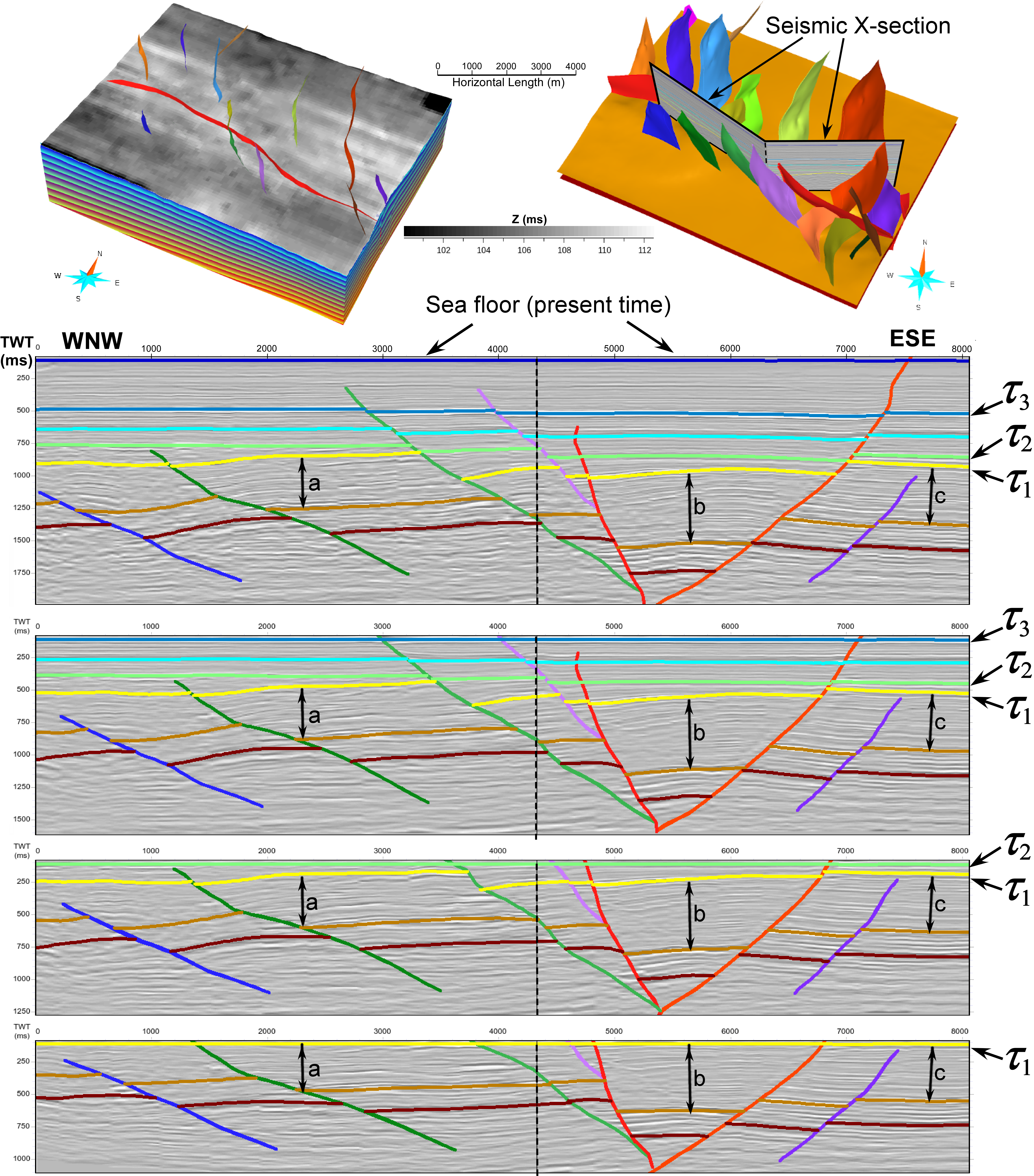
Figure 15: Restoration of several horizons in a three-dimensional model with an erosive stratigraphic sequence. Location of seismic image section is shown in top right corner. Sections below are painted with seismic image, faults and horizons in the present-day model and at three restoration times. Interval times between two horizons highlighted by thick, black arrows are preserved.

References

- Athy, (1930) Athy, L. F., 1930, Density, Porosity, and Compaction of Sedimentary Rocks, AAPG Bulletin, v. 14, no. 1, p. 1–24, doi: 10.1306/3D93289E-16B1-11D7-8645000102C1865D.
- Dahlstrom, (1969) Dahlstrom, C. D. A., 1969, Balanced cross sections, Canadian Journal of Earth Sciences, v. 6, no. 4, p. 743–757, doi: 10.1139/e69-069.
- Durand-Riard et al., (2010) Durand-Riard, P., G. Caumon, and P. Muron, 2010, Balanced restoration of geological volumes with relaxed meshing constraints, Computers & Geosciences, v. 36, no. 4, p. 441–452, doi: 10.1016/j.cageo.2009.07.007.
- Durand-Riard et al., (2013) Durand-Riard, P., C. Guzofski, G. Caumon, and M.-O. Titeux, 2013, Handling natural complexity in three-dimensional geomechanical restoration, with application to the recent evolution of the outer fold and thrust belt, deep-water Niger Delta, AAPG Bulletin, v. 97, no. 1, p. 87–102, doi: 10.1306/06121211136.
- Durand-Riard et al., (2011) Durand-Riard, P., L. Salles, M. Ford, G. Caumon, and J. Pellerin, 2011, Understanding the evolution of syn-depositional folds: Coupling decompaction and 3D sequential restoration, Marine and Petroleum Geology, v. 28, no. 8, p. 1530–1539, doi: 10.1016/j.marpetgeo.2011.04.001.
- Gibbs, (1983) Gibbs, A., 1983, Balanced cross-section construction from seismic sections in areas of extensional tectonics, Journal of Structural Geology, v. 5, no. 2, p. 153–160.
- Labbassi, (1999) Labbassi, K., 1999, Détermination des coefficients de compaction pour les faciès silico-clastiques et carbonatés du Bassin d’El Jadida-Agadir (Maroc), Géologie Méditerranéenne, v. 26, no. 1-2, p. 103–112, doi: 10.3406/geolm.1999.1650.
- Lovely et al., (2018) Lovely, P. J., S. N. Jayr, and D. A. Medwedeff, 2018, Practical and efficient three-dimensional structural restoration using an adaptation of the GeoChron model, AAPG Bulletin, v. 102, no. 10, p. 1985–2016, doi: 10.1306/03291817191.
- Maerten and Maerten, (2015) Maerten, F. and L. Maerten, 2015, On a method for reducing interpretation uncertainty of poorly imaged seismic horizons and faults using geomechanically based restoration technique, Interpretation, v. 3, no. 4, p. 105–116, doi: 10.1190/int-2015-0009.1.
- Mallet, (2014) Mallet, J.-L., 2014, Elements of Mathematical Sedimentary Geology: the GeoChron Model: Houten, EAGE Publications BV, 388 p.
- Moretti, (2008) Moretti, I., 2008, Working in complex areas: New restoration workflow based on quality control, 2D and 3D restorations, Marine and Petroleum Geology, v. 25, no. 3, p. 205–218, doi: 10.1016/j.marpetgeo.2007.07.001.
- Moretti et al., (2006) Moretti, I., F. Lepage, and M. Guiton, 2006, KINE3D: a New 3d Restoration Method Based on a Mixed Approach Linking Geometry and Geomechanics, Oil & Gas Science and Technology, v. 61, no. 2, p. 277–289, doi: 10.2516/ogst:2006021.
- Muron, (2005) Muron, P., 2005, Méthodes numériques 3-D de restauration des structures géologiques faillées, Ph.D. thesis, Institut National Polytechnique de Lorraine, Nancy, France, 131 p.
- Schneider et al., (1996) Schneider, F., J. Potdevin, S. Wolf, and I. Faille, 1996, Mechanical and chemical compaction model for sedimentary basin simulators, Tectonophysics, v. 263, no. 1-4, p. 307–317, doi: 10.1016/s0040-1951(96)00027-3.
- Sederberg and Parry, (1986) Sederberg, T. W. and S. R. Parry, 1986, Free-form deformation of solid geometric models, Computer Graphics, p. 151–160, doi: 10.1145/15922.15903.
- Suppe, (1985) Suppe, J., 1985, Principles of Structural Geology: Englewood Cliffs, NJ, Prentice-Hall, Inc., 537 p.
- Tertois and Mallet, (2019) Tertois, A.-L. and J.-L. Mallet, 2019, Restoration of Complex Three-Dimensional Structural Models Based on the Mathematical GeoChron Framework, In: 81st EAGE Conference and Exhibition 2019, EAGE Publications BV, doi: 10.3997/2214-4609.201901294.