House Price Prediction using Satellite Imagery

Abstract

In this paper we show how using satellite images can improve the accuracy of housing price estimation models. Using Los Angeles County’s property assessment dataset, by transferring learning from an Inception-v3 model pretrained on ImageNet, we could achieve an improvement of  10% in R-squared score compared to two baseline models that only use non-image features of the house.

1 Introduction

High-resolution satellite images from most of the Earth’s surface have been available for over a decade, and in recent years advanced deep learning methods have been applied to them. Mnih et. al. started this field with a classifier that detects roads [7]. More recently, deep learning models and satellite imagery have been used for more complicated tasks such as crop yield prediction in the U.S. [10] and poverty prediction in Africa [5].

We believe there are still many unexplored questions and potential applications for this field of study. One such problem is using satellite images to enhance existing house price prediction models, which historically only used hand-selected features (e.g. number of rooms or floor area). We show that a vision-based model can learn important relevant features from the neighborhood of a house (e.g. distance from green fields or highways) by processing a single satellite image, and then use those features to improve the estimation accuracy.

Although high-resolution satellite images contain an abundance of information that might be correlated with house prices, such data are highly unstructured and thus challenging to extract meaningful insights from. Although deep learning models such as convolutional neural networks (CNN) could in principle be trained to directly estimate prices from satellite imagery, the scarcity of training data makes the application of these techniques challenging. Therefore, we use transfer learning techniques to overcome this problem in that we will use knowledge gained while solving one problem and apply it to our different but related problem. We will start with a CNN model that has been trained on ImageNet [8], a large image classification data set, to identify low-level image features such as edges and corners that are common to many vision tasks. Next, we will build on the knowledge gained from this image classification task and fine-tune the model on a new task.

We combine a dataset of house prices (from LA County’s property assessment dataset ) and a dataset of satellite images (collected via Google Static Maps API ) to accomplish this objective. The input to our model is a $640\times 640$ image (with the house located at the center) and a feature vector (number of bedrooms, etc.). The output is a single number, the value of the house in dollars. We feed the image to the pretrained CNN whose last two layers have been deleted after pretraining, and get a feature vector for the image. We then combine the two feature vectors using several fully-connected layers and get the output.

Finally, we evaluate our estimation performance using $R^{2}$ and mean-squared error (MSE) metrics. The results will be compared to two baseline models that only use hand-selected features.

The inspiration for this project came from Zillow’s Home Value Prediction competition , which is challenging the data science community to help push the accuracy of the house price estimations further by utilizing any additional source of information .

2 Related work

Traditionally, house price prediction models used hand-selected features (e.g. number of rooms or floor area). Feed-forward neural networks and various decision-tree-based models [3] outperformed other approaches. However, as [2] mentions, the parameters that determine the price of a house are twofold: one that is intrinsic to the house and one that indicates the "desirability" of the house. Traditional models can only learn the former, but the latter usually depends on the location of the house [6]. In particular, social and economic metrics such as crime rate, pollution levels and distance from important locations (e.g. train station, hospitals) can affect the housing price [1]. Therefore, a model that is able to capture the resulting spatial correlations can potentially outperform other models. Spatial auto-regressive (SAR) models are one approach to capturing the existing spatial correlation in housing prices. These models rely on a spatial contiguity matrix that is usually hand-designed with the help of a domain expert, but as [2] showed, can also be learned by algorithms. Non of these models use vision-related features. More recently, [1] proposed a model that uses deep neural networks to extract information from satellite images, combined them with an SAR model and other house features. This approach resulted in a $57\%$ reduction in RMSE compared to a model with SAR but without satellite images.

It is worth noting that these papers use different datasets which in most cases are gathered by the authors of the paper. This makes it difficult to compare their results in a completely fair manner However, it can be seen that the focus of the research has been moving towards models that can capture features from outside the building itself, which has generally improved the accuracy of estimators.

3 Dataset and Features

Our dataset consists of two main parts: 1. real estate properties, and 2. high-resolution satellite images. Details of each part are explained in this section.

3.1 Real Estate Properties

We collected properties data from LA County’s property assessment data which is available online. This dataset consists of more than 2 million real-estate properties in LA county assessed between 2006 and 2017. Each entry had 50 features, floor area, number of bedrooms, year built, use type, latitude and longitude to name a few. Preprocessing was done on the data, details of which will be discussed later in this paper.

3.2 High-Resolution Satellite Images

To better predict the price error, we combined our main dataset with satellite images of houses, collected via Google Static Maps API using the longitude and latitude of each house. This API gives access to different zoom levels between 1 (the Earth) and 24 (the most detailed). In this study, we set the zoom level to 19, and retrieved images with size 640x640 which is the highest resolution available for the free tier users. Figure 1 shows a few examples. We believe this zoom level provides a suitable amount of information about the neighborhood while showing the shape of the building itself.

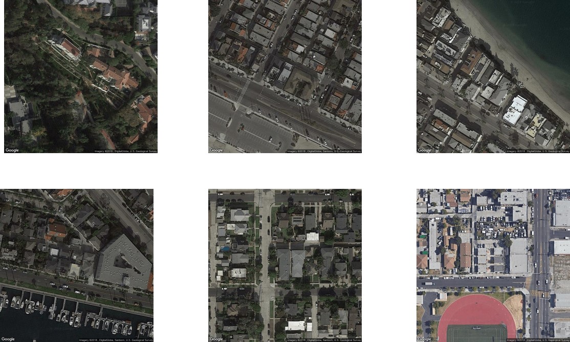
Figure 1: Examples of satellite images. Each image is $640\times 640$ pixels.

3.3 Data Preprocessing

Before beginning analysis, the LA County dataset was preprocessed. Eight columns contained unrelated information such as assessor’s ID and parcel ID, which were removed. One redundant column was also removed. With each property, came three price values: total land value, personal property value, and total value. In addition to residential properties, the data included rows for non-residential properties as well as empty lots. Since our aim is to study housing price estimations, we focused our analysis on entries for which personal property value was non-zero, and used this column as our labels. Consequently, non-residential rows were removed. Finally, we ended up with 40 features per property, among which 23 were categorical parameters (e.g. use type). We replaced categories with integer values. Each column in the dataset was then normalized to have zero mean and standard deviation of $1$. Table 1 shows a summary of the size of our dataset.

Train Set Size	Validation Set Size	Test Set Size	Number of Features
48,548	2,698	2,698	40

Table 1: Train/validation/test size of the dataset

4 Methods

4.1 Baseline Models

We started our analysis by building two baseline models: decision-tree-based models and neural networks. For the former, we analyzed multiple tree-based estimators. Extra tree regressor [4] demonstrated the best performance and was chosen as our baseline. Moreover, we trained a neural network on our features dataset. Performance of these models are provided in the Experiments and Results section.

4.2 Inception-v3

Since we do not have enough data to train vision-based convolutional neural networks, we use pretrained models to encode images. We use Inception-v3 model [9], trained on ImageNet, to construct 2048-dimensional vectors for our images. The process is as follows. First, JPEG satellite images are converted into RGB matrices, resized to $299\times 299\times 3$ and normalized to have values in $[0,1]$ to match the expected input of Inception-v3. Feeding the data into the model, we then save resulting vectors in a binary file to be used later in our network. This time-consuming process generated around 8 gigabytes of processed data. We do this in order to make the training process faster and be able to iterate more quickly in hyperparameter tuning part of the project.

4.3 Cost Function

We use mean-squared error (MSE) as our cost function: $J=\frac{1}{m}\sum_{i=1}^{m}L(\hat{y}^{(i)},y^{(i)})=\frac{1}{m}\sum_{i=1}^{m}(\hat{y}^{(i)}-y^{(i)})^{2}$. Note that we report our results using $R^{2}$ (not MSE), but the two metrics are nicely related in a way that minimizing MSE is equivalent to maximizing $R^{2}$: $R^{2}=1-\frac{MSE}{S}$ where $S$ is the variance of the test set’s labels.

5 Experiments and Results

5.1 Experiments

All numerical results are provided in table 2. We have studied to see if images alone are able to make estimations about prices. Encodings are fed into fully-connected neural network layers and trained to minimize mean squared error (MSE) loss.

From the results we got, it is apparent that by themselves, images are not able to predict prices. This can be attributed to the difficulty of estimations of house size from images. It is not possible for a model to decide on the size of a house by just looking at a satellite picture, as is may include several other buildings too.

Next step was to train models on both features and images to see if combining the two can improve our estimations. We feed our two feature vectors to two separate dense networks and we concatenate the results in the final layer. We will describe the details of this model in the Network Architecture section.

Model	Train $R^{2}$	Dev $R^{2}$	Test $R^{2}$	Train MSE	Dev MSE	Test MSE
Extra Tree (baseline)	0.99	0.86	0.71	0.000	0.112	0.002
Neural Net F (baseline)	0.96	0.84	0.85	0.037	0.136	0.001
Neural Net I	$0.000$	-0.0001	-0.038	1.062	0.859	0.010
Neural Net F+I	0.98	0.94	0.93	0.011	0.044	0.001

Table 2: Summary of results. MSE (mean-square error) is calculated using normalized labels. F is features, I is satellite images.

5.2 Interpretation of the Results

We see that the F+I model outperforms all other models by at least $10\%$ in $R^{2}$ metric. Intuitively, the cost of a house is approximately floor area $\times$ price per square foot. While features provide the model with the first factor, images help it improve its estimation for the second. We ranked data points based on how much F+I improves estimations compared to F model. Top 5 positive (F+I corrected underestimation) and top 4 negative improvements (F+I improved overestimation) are shown in figures 2 and 3 respectively.

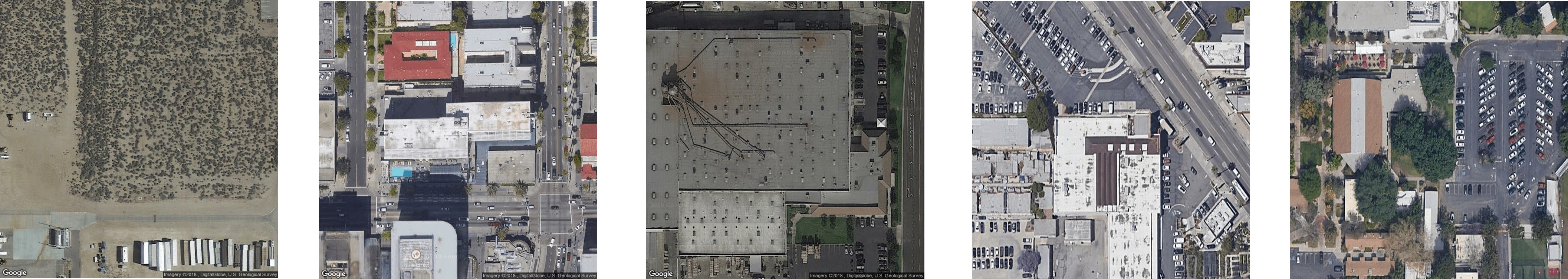
Figure 2: Baselines underestimated the price of these houses and F+I corrected them.

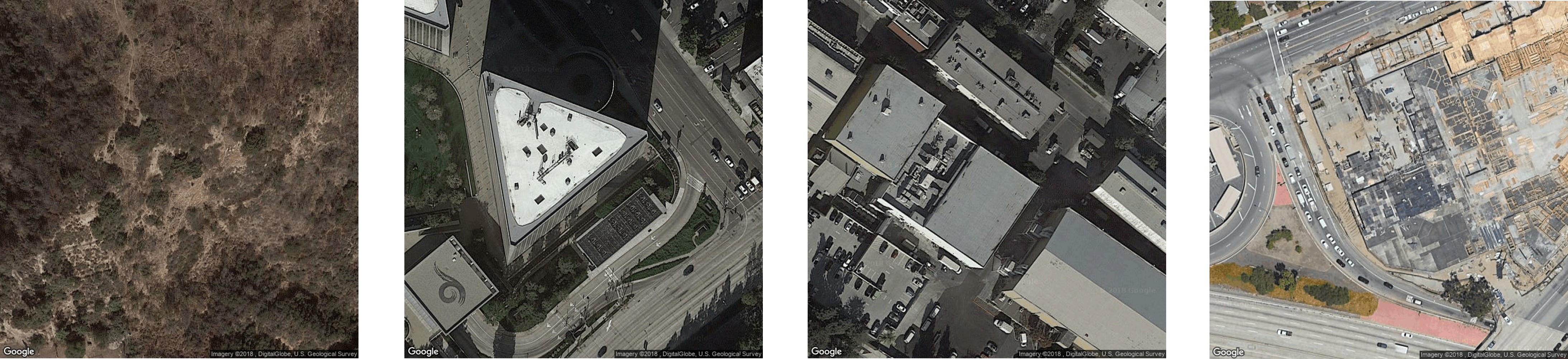
Figure 3: Baselines overestimated the price of these houses and F+I corrected them.

An interesting observation is that our dataset -despite all the preprocessing that we have done- contained a few empty lands with no buildings. The fact that these data points are present in figures 2 and 3 shows that our model is more robust to noise in the data. After evaluating figure 2, we think it shows that our model realizes that cars are an indicator of higher prices (since it shows higher accessibility or low distance from city center), so it adds to the estimated price.

5.3 Network Architecture

We have tried many different architectures and hyperparameters, and in this section only describe the best results. Also, due to lack of space we only describe our model for F+I model. We use the architecture described in figure 4. The hyper parameters are mentioned in table 3. Our model, especially on image side is very prone to over-fitting, so we use L2 regularization and dropout to prevent that. The learning rate (lr) is decreased after each batch is processed, using the following formula: $lr=\frac{lr}{1+\alpha\times t}$. We use a relatively big batch size because we were training on a GPU. Larger batch sizes (but smaller than available memory size) help increase the utilization of GPU and generally speed up the training process.

L2 Regularization Parameter	$0.1$
First Dropout (drop probability)	$0.3$
First Dropout (drop probability)	$0.2$
Activation Function	ReLU
Batch Size	$1024$
Optimizer	Adam(learning rate=$0.0005$, $\beta_{1}=0.9$, $\beta_{2}=0.999$)
Epochs	$200$
Learning Rate Decay	$\alpha=0.0001$

Table 3: Hyperparameters for F+I model

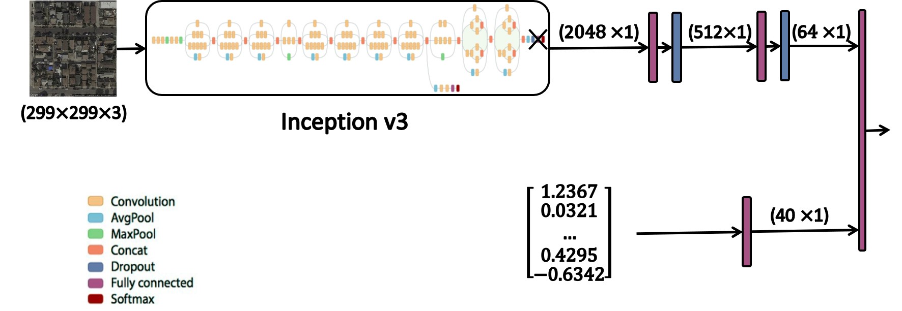
Figure 4: F+I neural network architecture

6 Conclusion/Future Work

To sum up, by adding satellite images to our prediction model, we were able to improve $R^{2}$ by  10% and reduce MSE by  60% compared to the baseline. The results are promising. We believe the following future steps are worth further analysis.

Using different image zoom levels or a combination of them: Lower zoom levels will be able to capture more details about the neighborhood as they cover a wider range around the property, while a higher zoom level may estimate based on more details from the house, for example the materials used to build it. Fine tuning last layers of the Inception-v3 network: Inception-v3 encodes images of size 299x299x3 to 2048-dimensional vectors. Thus, valuable information may be omitted by this process. As a future step, we can take outputs of earlier layers of the pretrained model or fine tune parameters of the last few convolutional layers. This will allow us to capture more relevant features from the images. Adding data from different locations to the dataset to test how generalizable the model is from one location to another: Since public data of property transactions are widely available today, analysis can continue on larger datasets consisting of more counties. This will add to inputs’ variance, and potentially make the model more robust. We can then examine if our approach can be generalized.

References

- Bency et al. [2016] A. J. Bency, S. Rallapalli, R. K. Ganti, M. Srivatsa, and B. S. Manjunath. Beyond Spatial Auto-Regressive Models: Predicting Housing Prices with Satellite Imagery. 2016. URL http://arxiv.org/abs/1610.04805.
- Chopra et al. [2007] S. Chopra, T. Thampy, J. Leahy, A. Caplin, and Y. LeCun. Discovering the hidden structure of house prices with a non-parametric latent manifold model. Proceedings of the 13th ACM SIGKDD international conference on Knowledge discovery and data mining - KDD ’07, page 173, 2007. doi: 10.1145/1281192.1281214. URL http://portal.acm.org/citation.cfm?doid=1281192.1281214.
- Fan et al. [2006] G.-Z. Fan, S. E. Ong, and H. C. Koh. Determinants of House Price: A Decision Tree Approach. Urban Studies, 43(12):2301–2315, 2006. ISSN 00420980. doi: 10.1080/00420980600990928. URL http://proxy.elmhurst.edu/login?url=http://search.ebscohost.com/login.aspx?direct=true{&}db=a9h{&}AN=23148559{&}site=ehost-live.
- Geurts et al. [2006] P. Geurts, D. Ernst, and L. Wehenkel. Extremely randomized trees. Machine Learning, 63(1):3–42, 2006. ISSN 08856125. doi: 10.1007/s10994-006-6226-1.
- Jean et al. [2016] N. Jean, M. Burke, M. Xie, W. M. Davis, D. B. Lobell, and S. Ermon. Combining satellite imagery and machine learning to predict poverty. Science, 353(6301):790–794, 2016. ISSN 0036-8075. doi: 10.1126/science.aaf7894. URL http://science.sciencemag.org/content/353/6301/790.
- Kockelman [1997] K. Kockelman. Effects of Location Elements on Home Purchase Prices and Rents in San Francisco Bay Area. Transportation Research Record: Journal of the Transportation Research Board, 1606(-1):40–50, 1997. ISSN 0361-1981. doi: 10.3141/1606-06. URL http://dx.doi.org/10.3141/1606-06.
- Mnih and Hinton [2010] V. Mnih and G. E. Hinton. Learning to detect roads in high-resolution aerial images. In K. Daniilidis, P. Maragos, and N. Paragios, editors, Computer Vision – ECCV 2010, pages 210–223, Berlin, Heidelberg, 2010. Springer Berlin Heidelberg. ISBN 978-3-642-15567-3.
- Russakovsky et al. [2015] O. Russakovsky, J. Deng, H. Su, J. Krause, S. Satheesh, S. Ma, Z. Huang, A. Karpathy, A. Khosla, M. Bernstein, A. C. Berg, and L. Fei-Fei. Imagenet large scale visual recognition challenge. International Journal of Computer Vision, 115(3):211–252, Dec 2015. ISSN 1573-1405. doi: 10.1007/s11263-015-0816-y. URL https://doi.org/10.1007/s11263-015-0816-y.
- Szegedy et al. [2015] C. Szegedy, V. Vanhoucke, S. Ioffe, J. Shlens, and Z. Wojna. Rethinking the Inception Architecture for Computer Vision. 2015. ISSN 08866236. doi: 10.1109/CVPR.2016.308. URL http://arxiv.org/abs/1512.00567.
- You et al. [2017] J. You, X. Li, M. Low, D. Lobell, and S. Ermon. Deep Gaussian Process for Crop Yield Prediction Based on Remote Sensing Data. 2017 Association for the Advancement of Articial Intelligence, pages 4559–4565, 2017.