DataExposer: Exposing Disconnect between Data and Systems

Abstract.

As data is a central component of many modern systems, the cause of a system malfunction may reside in the data, and, specifically, particular properties of the data. For example, a health-monitoring system that is designed under the assumption that weight is reported in imperial units (lbs) will malfunction when encountering weight reported in metric units (kilograms). Similar to software debugging, which aims to find bugs in the mechanism (source code or runtime conditions), our goal is to debug the data to identify potential sources of disconnect between the assumptions about the data and the systems that operate on that data. Specifically, we seek which properties of the data cause a data-driven system to malfunction. We propose DataExposer, a framework to identify data properties, called profiles, that are the root causes of performance degradation or failure of a system that operates on the data. Such identification is necessary to repair the system and resolve the disconnect between data and system. Our technique is based on causal reasoning through interventions: when a system malfunctions for a dataset, DataExposer alters the data profiles and observes changes in the system’s behavior due to the alteration. Unlike statistical observational analysis that reports mere correlations, DataExposer reports causally verified root causes—in terms of data profiles—of the system malfunction. We empirically evaluate DataExposer on three real-world and several synthetic data-driven systems that fail on datasets due to a diverse set of reasons. In all cases, DataExposer identifies the root causes precisely while requiring orders of magnitude fewer interventions than prior techniques.

PVLDB Reference Format:
DataExposer: Exposing Disconnect between Data and Systems. PVLDB, 14(1): XXX-XXX, 2020.
doi:XX.XX/XXX.XX

1. Introduction

Traditional software debugging aims to identify errors and bugs in the mechanism—such as source code, configuration files, and runtime conditions—that may cause a system to malfunction (Hailpern and Santhanam, 2002; Liblit et al., 2005; Fariha et al., 2020). However, in modern systems, data has become a central component that itself can cause a system to fail. Data-driven systems comprise complex pipelines that rely on data to solve a target task. Prior work addressed the problem of debugging machine-learning models (Cadamuro et al., 2016) and finding root causes of failures in computational pipelines (Lourenço et al., 2020), where certain values of the pipeline parameters—such as a specific model and/or a specific dataset—cause the pipeline failure. However, just knowing that a pipeline fails for a certain dataset is not enough; naturally, we ask: what properties of a dataset caused the failure?

Two common reasons for malfunctions in data-driven systems are: (1) incorrect data, and (2) disconnect between the assumptions about the data and the design of the system that operates on the data. Such disconnects may happen when the system is not robust, i.e., it makes strict assumptions about metadata (e.g., data format, domains, ranges, and distributions), and when new data drifts from the data over which the system was tested on before deployment (Rawal et al., 2020) (e.g., when a system expects a data stream to have a weekly frequency, but the data provider suddenly switches to daily data).

Therefore, in light of a failure, one should investigate potential issues in the data. Some specific examples of commonly observed system malfunctions caused by data include: (1) decline of a machine-learned model’s accuracy (due to out-of-distribution data), (2) unfairness in model predictions (due to imbalanced training data), (3) excessive processing time (due to a system’s failure to scale to large data), and (4) system crash (due to invalid input combination in the data tuples beyond what the system was designed to handle). These examples indicate a common problem: disconnect or mismatch between the data and the system design. Once the mismatch is identified, then possible fixes could be either to repair the data to suit the system design, or to adjust the system design (e.g., modify source code) to accommodate data with different properties.

A naïve approach to deal with potential issues in the data is to identify outliers: report tuples as potentially problematic based on how atypical they are with respect to the rest of the tuples in the dataset. However, without verifying whether the outliers actually cause unexpected outcomes, we can never be certain about the actual root causes. As pointed out in prior work (Barowy et al., 2014): “With respect to a computation, whether an error is an outlier in the program’s input distribution is not necessarily relevant. Rather, potential errors can be spotted by their effect on a program’s output distribution.” To motivate our work, we start with an example taken from a real-world incident, where Amazon’s delivery service was found to be racist (Is Amazon same-day delivery service racist?, 2016).

Example 1 (Biased Classifier).

An e-commerce company wants to build an automated system that suggests who should get discounts. To this end, they collect information from the customers’ purchases over one year and build a dataset over the attributes name, gender, age, race, zip_code, phone, products_purchased, etc. Anita, a data scientist, is then asked to develop a machine learning (ML) pipeline over this dataset to predict whether a customer will spend over a certain amount, and, subsequently, should be offered discounts. Within this pipeline, Anita decides to use a logistic regression classifier for prediction and implements it using an off-the-shelf ML library. To avoid discrimination over any group and to ensure that the classifier trained on this dataset is fair, Anita decides to drop the sensitive attributes—race and gender—during the pre-processing step of the ML pipeline, before feeding it to the classifier. However, despite this effort, the trained classifier turns out to be highly biased against African American people and women. After a close investigation, Anita discovers that: (1) In the training data, race is highly correlated with zip_code, and (2) The training dataset is imbalanced: a larger fraction of the people who purchase expensive products are male. Now she wonders: if these two properties did not hold in the dataset, would the learned classifier be fair? Have either (or both) of these properties caused the observed unfairness?

Unfortunately, existing tools (e.g., CheckCell (Barowy et al., 2014)) that blame individual cells (values) for unexpected outcomes cannot help here, as no single cell in the training data is responsible for the observed discrimination, rather, global statistical properties (e.g., correlation) that involve multiple attributes over the entire data are the actual culprits. Furthermore, Anita only identified two potential or correlated data issues that may or may not be the actual cause of the unfairness. To distinguish mere correlation from true causation and to verify if there is indeed a causal connection between the data properties and the observed unfairness, we need to dig deeper.

Example 1 is one among many incidents in real-world applications where issues in the data caused systems to malfunction (Bias, ring; Google, cism). A recent study of 112 high-severity incidents in Microsoft Azure services showed that 21% of the bugs were due to inconsistent assumptions about data format by different software components or versions (Liu et al., 2019). The study further found that 83% of the data-format bugs were due to inconsistencies between data producers and data consumers, while 17% were due to mismatch between interpretations of the same data by different data consumers. Similar incidents happened due to misspelling and incorrect date-time format (Rezig et al., 2020b), and issues pertaining to data fusion where schema assumptions break for a new data source (Dong et al., 2014; Wang et al., 2015). We provide another illustrative example where a system times out when the distribution of the data, over which the system operates, exhibits significant skew.

Example 2 (Process Timeout).

A toll collection software EZGo checks if vehicles passing through a gate have electronic toll pass installed. If it fails to detect a toll pass, it uses an external software OCR to extract the registration number from the vehicle’s license plate. EZGo operates in a batch mode and processes every $1000$ vehicles together by reserving AWS for one hour, assuming that one hour is sufficient for processing each batch. However, for some batches, EZGo fails. After a close investigation, it turns out that the external software OCR uses an algorithm that is extremely slow for images of black license plates captured in low illumination. As a result, when a batch contains a large number of such cases (significantly skewed distribution), EZGo fails.

The aforementioned examples bring forth two key challenges. First, we need to correctly identify potential causes of unexpected outcomes and generate hypotheses that are expressive enough to capture the candidate root causes. For example, “outliers cause unexpected outcomes” is just one of the many possible hypotheses, which offers very limited expressivity. Second, we need to verify the hypotheses to confirm or refute them, which enables us to pinpoint the actual root causes, eliminating false positives.

Data profile as root cause.

Towards solving the first challenge, our observation is that data-driven systems often function properly for certain datasets, but malfunction for others. Such malfunction is often rooted in certain properties of the data, which we call data profiles, that distinguish passing and failing datasets. Examples include size of a dataset, domains and ranges of attribute values, correlations between attribute pairs, conditional independence (Yan et al., 2020), functional dependencies and their variants (Papenbrock et al., 2015a; Koudas et al., 2009; Fan et al., 2009; Ilyas et al., 2004; Caruccio et al., 2016), and other more complex data profiles (Song and Chen, 2011; Langer and Naumann, 2016; Papenbrock et al., 2015b; Chu et al., 2013).

Oracle-guided root cause identification.

Our second observation is that if we have access to an oracle that can indicate whether the system functions desirably or not, we can verify our hypotheses. Access to an oracle allows us to precisely isolate the correct root causes of the undesirable malfunction from a set of candidate causes. Here, an oracle is a mechanism that can characterize whether the system functions properly over the input data. The definition of proper functioning is application-specific; for example, achieving a certain accuracy may indicate proper functioning for an ML pipeline. Such oracles are often available in many practical settings, and have been considered in prior work (Lourenço et al., 2020; Fariha et al., 2020).

Solution sketch. In this paper, we propose DataExposer, a framework that identifies and exposes data profiles that cause a data-driven system to malfunction. Our framework involves two main components: (1) an intervention-based mechanism that alters the profiles of a dataset, and (2) a mechanism that speeds up analysis by carefully selecting appropriate interventions. Given a scenario where a system malfunctions (fails) over a dataset but functions properly (passes) over another, DataExposer focuses on the discriminative profiles, i.e., data profiles that significantly differ between the two datasets. DataExposer’s intervention mechanism modifies the “failing” dataset to alter one of the discriminative profiles; it then observes whether this intervention causes the system to perform desirably, or the malfunction persists. DataExposer speeds up this analysis by favoring interventions on profiles that are deemed more likely causes of the malfunction. To estimate this likelihood, we leverage three properties of a profile: (1) coverage: the more tuples an intervention affects, the more likely it is to fix the system behavior, (2) discriminating power: the bigger the difference between the failing and the passing datasets over a profile, the more likely that the profile is a cause of the malfunction, and (3) attribute association: if a profile involves an attribute that is also involved with a large number of other discriminative profiles, then that profile has high likelihood to be a root cause. This is because altering such a profile is likely to passively repair other discriminative profiles as a side-effect (through the associated attribute). We also provide a group-testing-based technique that allows group intervention, which helps expedite the root-cause analysis further.

Scope. In this work, we assume knowledge of the classes of (domain-specific) data profiles that encompass the potential root causes. E.g., in Example 1, we assume the knowledge that correlation between attribute pairs and disparity between the conditional probability distributions (the probability of belonging to a certain gender, given price of items bought) are potential causes of malfunction. This assumption is realistic because: (1) For a number of tasks there exists a well-known set of relevant profiles: e.g., class imbalance and correlation between sensitive and non-sensitive attributes are common causes of unfairness in classification (Bellamy et al., 2018); and violation of conformance constraints (Fariha et al., 2021), missing values, and out-of-distribution tuples are well-known causes of ML model’s performance degradation. (2) Domain experts are typically aware of the likely class of data profiles for the specific task at hand and can easily provide this additional knowledge as a conservative approximation, i.e., they can include extra profiles just to err on the side of caution. Notably, this assumption is also extremely common in software debugging techniques (Fariha et al., 2020; Liblit et al., 2005; Zheng et al., 2006), which rely on the assumption that the “predicates” (traps to extract certain runtime conditions) are expressive enough to encode the root causes, and software testing (Mesbah et al., 2011), validation (Kumar et al., 2013), and verification (Henzinger et al., 2003) approaches, which rely on the assumption that the test cases, specifications, and invariants reasonably cover the codebase and correctness constraints.

To support a data profile, DataExposer further needs the corresponding mechanisms for discovery and intervention. In this work, we assume knowledge of the profile discovery and intervention techniques, as they are orthogonal to our work. Nevertheless, we discuss some common classes of data profiles supported in DataExposer and the corresponding discovery and intervention techniques. For data profile discovery, we rely on prior work on pattern discovery (Python, kage), statistical-constraint discovery (Yan et al., 2020), data-distribution learning (Hellerstein, 2008), knowledge-graph-based concept identification (Galhotra et al., 2019), etc. While our evaluation covers specific classes of data profiles (for which there exist efficient discovery techniques), our approach is generic and works for any class of data profiles, as long as the corresponding discovery and intervention techniques are available.

Limitations of prior work. To find potential issues in data, Dagger (Rezig et al., 2020b, a) provides data debugging primitives for human-in-the-loop interactions with data-driven computational pipelines. Other explanation-centric efforts (Wang et al., 2015; Bailis et al., 2017; Chirigati et al., 2016; El Gebaly et al., 2014) report salient properties of historical data based only on observations. In contrast with observational techniques, the presence of an oracle allows for interventional techniques (Lourenço et al., 2020) that can query the oracle with additional, system-generated test cases to identify root causes of system malfunction more accurately. One such approach is CheckCell (Barowy et al., 2014), which presents a ranked list of cells of data rows that unusually affect output of a given target function. CheckCell uses a fine-grained approach: it removes one cell of the data at a time, and observes changes in the output distribution. While it is suitable for small datasets, where it is reasonable to expect a human-in-the-loop paradigm to fix cells one by one, it is not suitable for large datasets, where no individual cell is significantly responsible, rather, a holistic property of the entire dataset (profile) causes the problem.

Interpretable machine learning is related to our problem, where the goal is to explain behavior of machine-learned models. However, prior work on interpretable machine learning (Ribeiro et al., 2016, 2018) typically provide local (tuple-level) explanations, as opposed to global (dataset-level) explanations. While some approaches provide feature importance as a global explanation for model behavior (Casalicchio et al., 2018), they do not model feature interactions as possible explanations.

Software testing and debugging techniques (Gulzar et al., 2018; Attariyan and Flinn, 2011; Attariyan et al., 2012; Chen et al., 2002; Fraser and Arcuri, 2013; Godefroid et al., 2008; Holler et al., 2012; Johnson et al., 2020; Zheng et al., 2006; Liblit et al., 2005) are either application-specific, require user-defined test suites, or rely only on observational data. The key contrast between software debugging and our setting is that the former focuses on white-box programs: interventions, runtime conditions, program invariants, control-flow graphs, etc., all revolve around program source code and execution traces. Unlike programs, where lines have logical and semantic connections, tuples in data do not have similar associations. Data profiles significantly differ in their semantics, and discovery and intervention techniques from program profiles, and, thus, techniques for program profiling do not trivially apply here. We treat data as a first-class citizen in computational pipelines, while considering the program as a black box.

Contributions. In this paper, we make the following contributions:

• We formalize the novel problem of identifying root causes (and fixes) of the disconnect between data and data-driven systems in terms of data profiles (and interventions). (Sec 2)

• We design a set of data profiles that are common root causes of data-driven system malfunctions, and discuss their discovery and intervention techniques based on available technology. (Sec 3)

• We design and develop a novel interventional approach to pinpoint causally verified root causes. The approach leverages a few properties of the data profiles to efficiently explore the space of candidate root causes with a small number of interventions. Additionally, we develop an efficient group-testing-based algorithm that further reduces the number of required interventions. (Sec 4)

• We evaluate DataExposer on three real-world applications, where data profiles are responsible for causing system malfunction, and demonstrate that DataExposer successfully explains the root causes with a very small number of interventions (¡ $5$). Furthermore, DataExposer requires $10$–$1000\times$ fewer interventions when compared against two state-of-the-art techniques for root-cause analysis: BugDoc (Lourenço et al., 2020) and Anchors (Ribeiro et al., 2018). Through an experiment over synthetic pipelines, we further show that the number of required interventions by DataExposer increases sub-linearly with the number of discriminative profiles, thanks to our group-testing-based approach. (Sec 5)

2. Preliminaries & Problem Definition

In this section, we first formalize the notions of system malfunction and data profile, its violation, and transformation function used for intervention. We then proceed to define explanation (cause and corresponding fix) of system malfunction and formulate the problem of data-profile-centric explanation of system malfunction.

Basic notations. We use $\mathcal{R}(A_{1},A_{2},\dots,A_{m})$ to denote a relation schema over $m$ attributes, where $A_{i}$ denotes the $i^{th}$ attribute. We use $\texttt{Dom}_{i}$ to denote the domain of attribute $A_{i}$. Then the set ${\mathbf{Dom}}^{m}=\texttt{Dom}_{1}\times\cdots\times\texttt{Dom}_{m}$ specifies the domain of all possible tuples. A dataset $D\subseteq{\mathbf{Dom}}^{m}$ is a specific instance of the schema $\mathcal{R}$. We use $t\in\mathbf{Dom}^{m}$ to denote a tuple in the schema $\mathcal{R}$. We use $t.A_{i}\in\texttt{Dom}_{i}$ to denote the value of the attribute $A_{i}$ of the tuple $t$ and use $D.A_{j}$ to denote the multiset of values all tuples in $D$ take for attribute $A_{j}$.

2.1. Quantifying System Malfunction

To measure how much the system malfunctions over a dataset, we use the malfunction score.

Definition 1 (Malfunction score).

Let $D\subseteq\mathbf{Dom}^{m}$ be a dataset, and $S$ be a system operating on $D$. The malfunction score $m_{S}(D)\in[0,1]$ is a real value that quantifies how much $S$ malfunctions when operating on $D$.

The malfunction score $m_{S}(D)=0$ indicates that $S$ functions properly over $D$ and a higher value indicates a higher degree of malfunction, with $1$ indicating extreme malfunction. A threshold parameter $\tau$ defines the acceptable degree of malfunction and translates the continuous notion of malfunction to a Boolean value. If $m_{S}(D)\leq\tau$, then $D$ is considered to pass with respect to $S$; otherwise, there exists a mismatch between $D$ and $S$, whose cause (and fix) we aim to expose.

Example 2.

For a binary classifier, its misclassification rate (additive inverse of accuracy) over a dataset can be used as a malfunction score. Given a dataset $D$, if a classifier $S$ makes correct predictions for tuples in $D^{\prime}\subseteq D$ , and incorrect predictions for the remaining tuples, then $S$ achieves accuracy $\frac{\lvert D^{\prime}\rvert}{\lvert D\rvert}$, and, thus, $m_{S}(D)=1-\frac{\lvert D^{\prime}\rvert}{\lvert D\rvert}$.

Example 3.

In fair classification, we can use disparate impact (IBM, 360), which is defined by the ratio between the number of tuples with favorable outcomes within the unprivileged and the privileged groups, to measure malfunction.

2.2. Profile-Violation-Transformation (PVT)

Once we detect existence of a mismatch, the next step is to investigate its cause. We characterize the issues in a dataset that are responsible for the mismatch between the dataset and the system using data profiles. Structure or schema of data profiles is given by profile templates, which contains holes for parameters. Parameterizing a profile template gives us a concretization of the corresponding profile ($P$). Given a dataset $D$, we use existing data-profiling techniques to find out parameter values to obtain concretized data profiles, such that $D$ satisfies the concretized profiles. To evaluate how much a dataset $D$ satisfies or violates a data profile, we need a corresponding violation function ($V$). Violation functions provide semantics of the data profiles. Finally, to alter a dataset $D$, with respect to a data profile and the corresponding violation function, we need a transformation function ($T$). Transformation functions provide the intervention mechanism to alter data profiles of a dataset and suggest fix to remove the cause of malfunction. DataExposer requires the following three components over the schema $\langle$Profile, Violation function, Transformation function$\rangle$, PVT in short:

1. $P$: a (concretized) profile along with its parameters, which follows the schema $\langle$profile type, parameters$\rangle$.

2. $V(D,P)$: a violation function that computes how much the dataset $D$ violates the profile $P$ and returns a violation score.

3. $T(D,P,V)$: a transformation function that transforms the dataset $D$ to another dataset $D^{\prime}$ such that $D^{\prime}$ no longer violates the profile $P$ with respect to the violation function $V$. (When clear from the context, we omit the parameters $P$ and $V$ when using the notation for transformation functions.)

For a PVT triplet $X$, we define $X_{P}$ as its profile, $X_{V}$ as the violation function and $X_{T}$ as the transformation function. We provide examples and additional discussions on data profiles, violation functions, and transformation functions in Section 3.

2.2.1. Data Profile

Intuitively, data profiles encode dataset characteristics. They can refer to a single attribute (e.g., mean of an attribute) or multiple attributes (e.g., correlation between a pair of attributes, functional dependencies, etc.).

Definition 4 (Data Profile).

Given a dataset $D$, a data profile $P$ denotes properties or constraints that tuples in $D$ (collectively) satisfy.

2.2.2. Profile Violation Function

To quantify the degree of violation a dataset incurs with respect to a data profile, we use a profile violation function that returns a numerical violation score.

Definition 5 (Profile violation function).

Given a dataset $D$ and a data profile $P$, a profile violation function $V(D,P)\mapsto[0,1]$ returns a real value that quantifies how much $D$ violates $P$.

$V(D,P)=0$ implies that $D$ fully complies with $P$ (does not violate it at all). In contrast, $V(D,P)>0$ implies that $D$ violates $P$. The higher the value of $V(D,P)$, the higher the profile violation.

		Profile	Data type	Discovery over $D$	Interpretation	Violation by $D$	Transformation function
	$\mathbf{1}$	$\langle$Domain, $A_{j}$, $\mathbb{S}\rangle$	Categorical	$\mathbb{S}=\displaystyle\bigcup_{t\in D}\{t.A_{j}\}$	Values are drawn from a specific domain.	$\frac{\sum_{t\in D}\llbracket t.A_{j}\;\not\in\;\mathbb{S}\rrbracket}{\lvert D\rvert}$	Map values outside $\mathbb{S}$ to values in $\mathbb{S}$ using domain knowledge.
	$\mathbf{2}$	$\langle$Domain, $A_{j}$, $\mathbb{S}\rangle$	Numerical	$\mathbb{S}$ = $[\mathtt{lb},\mathtt{ub}]$, where $\mathtt{lb}$ = $\displaystyle\min_{t\in D}t.A_{j}$ $\mathtt{ub}$ = $\displaystyle\max_{t\in D}t.A_{j}$	Values lie within a bound.	$\frac{\sum_{t\in D}\llbracket t.A_{j}\;\not\in\;\mathbb{S}\rrbracket}{\lvert D\rvert}$	(1) Use monotonic linear transformation and transform all values. (2) Use winsorization techniques to replace the violating values only.
strict	$\mathbf{3}$	$\langle$Domain, $A_{j}$, $\mathbb{S}\rangle$	Text	$\mathbb{S}=[t\in\texttt{Dom}_{j}\mid t\models\mathbb{P}]$, where $\mathbb{P}$ is a regex over $D.A_{j}$ learned via pattern discovery (Python, kage)	Values satisfy a regular expression or length of values lie within a bound.	$\frac{\sum_{t\in D}\llbracket t.A_{j}\;\not\in\;\mathbb{S}\rrbracket}{\lvert D\rvert}$	Minimally alter data to satisfy regular expression. For example, insert (remove) characters to increase (reduce) text length.
	$\mathbf{4}$	$\langle$Outlier, $A_{j}$, $O$, $\theta\rangle$	All	$\theta=\frac{\sum_{t\in D}\llbracket O(D.A_{j},t.A_{j})\rrbracket}{\lvert D\rvert}$, where $O$ is learned from $D.A_{j}$’s distribution (Hellerstein, 2008)	Fraction of outliers within an attribute does not exceed a threshold.	$\max\Big{(}0,\frac{\sum_{t\in D}\llbracket O(D.A_{j},t.A_{j})\rrbracket-\theta\cdot\lvert D\rvert}{\lvert D\rvert\cdot(1-\theta)}\Big{)}$	(1) Replace outliers with the expected value (mean, median, mode) of the attribute. (2) Map all values above (below) the maximum (minimum) limit with highest (lowest) valid value.
	$\mathbf{5}$	$\langle$Missing, $A_{j}$, $\theta\rangle$	All	$\theta=\frac{\sum_{t\in D}\llbracket t.A_{j}=\mathtt{NULL}\rrbracket}{\lvert D\rvert}$	Fraction of missing values within an attribute does not exceed a threshold.	$\max\Big{(}0,\frac{\sum_{t\in D}\llbracket t.A_{j}=\mathtt{NULL}\rrbracket-\theta\cdot\lvert D\rvert}{\lvert D\rvert\cdot(1-\theta)}\Big{)}$	Use missing value imputation techniques.
thresholded by data coverage	$\mathbf{6}$	$\langle$Selectivity, $\mathbb{{P}},\theta\rangle$	All	$\theta=\frac{\lvert\sigma_{\mathbb{P}}(D)\rvert}{\lvert D\rvert}$	Fraction of tuples satisfying a given constraint (selection predicate) does not exceed a threshold.	$\max\Big{(}0,\frac{\lvert\sigma_{\mathbb{P}}(D)\rvert-\theta\cdot\lvert D\rvert}{\lvert D\rvert\cdot(1-\theta)}\Big{)}$	Undersample tuples that satisfy the predicate $\mathbb{P}$.
	$\mathbf{7}$	$\langle$Indep, $A_{j}$, $A_{k}$, $\alpha\rangle$	Categorical	$\alpha$ denotes Chi-squared statistic between $D.A_{j}$ and $D.A_{k}$	$\chi^{2}$ statistic between a pair of attributes is below a threshold with a p-value $\leq$ 0.05.	$1-e^{-\max(0,\chi^{2}(D.A_{j},D.A_{k})-\alpha)}$	Modify attribute values to remove/reduce dependence.
	$\mathbf{8}$	$\langle$Indep, $A_{j}$, $A_{k}$, $\alpha\rangle$	Numerical	$\alpha$ denotes Pearson correlation coefficient between $D.A_{j}$ and $D.A_{k}$	PCC between a pair attributes is below a threshold with a p-value $\leq$ 0.05.	$\max\big{(}0,\frac{\lvert\mathtt{PCC}(D.A_{j},D.A_{k})\rvert-\lvert\alpha\rvert}{1-\lvert\alpha\rvert}\big{)}$	Add noise to remove/reduce dependence between attributes.
thresholded by parameter	$\mathbf{9}$	$\langle$Indep, $A_{j}$, $A_{k},\alpha\rangle$	Categorical, numerical	Learn causal graph and causal coefficients ($\alpha$) using TETRAD (Scheines et al., 1998)	A causal relationship between a pair of attributes is unlikely (with causal coefficient less than $\alpha$).	$\max\big{(}0,\frac{|\mathtt{coeff}(A_{j},A_{k})|-\alpha}{1-\alpha}\big{)}$	Change data distribution to modify the causal relationship.

Figure 1. A list of PVT triplets that we consider in this paper, their syntax, and semantics.

2.2.3. Transformation Function

In our work, we assume knowledge of a passing dataset for which the system functions properly, and a failing dataset for which the system malfunctions. Our goal is to identify which profiles of the failing dataset caused the malfunction. We seek answer to the question: how to “fix” the issues within the failing dataset such that the system no longer malfunctions on it (mismatch is resolved)? To this end, we apply interventional causal reasoning: we intervene on the failing dataset by altering its attributes such that the profile of the altered dataset matches the corresponding correct profile of the passing dataset. To perform intervention, we need transformation functions with the property that it should push the failing dataset “closer” to the passing dataset in terms of the profile that we are interested to alter. More formally, after the transformation, the profile violation score should decrease.

Definition 6 (Transformation function).

Given a dataset $D$, a data profile $P$, and a violation function $V$, a transformation function $T(D,P,V)\mapsto 2^{\mathbf{Dom}^{m}}$ alters $D$ to produce $D^{\prime}$ such that $V(D^{\prime},P)=0$.

A dataset can be transformed by applying a series of transformation functions, for which we use the composition operator ($\circ$).

Definition 7 (Composition of transformations).

Given a dataset $D$, and two PVT triplets $X$ and $Y$, $(X_{T}\circ Y_{T})(D)=X_{T}(Y_{T}(D))$. Further, if $D^{\prime\prime}=(X_{T}\circ Y_{T})(D)$, then $X_{V}(D^{\prime\prime},X_{P})=Y_{V}(D^{\prime\prime},Y_{P})=0$.

2.3. Problem Definition

We expose a set of PVT triplets for explaining the system malfunction. The explanation contains both the cause and the corresponding fix: profile within a PVT triplet indicates the cause of system malfunction with respect to the corresponding transformation function, which suggests the fix.

Definition 8 (Explanation of system malfunction).

Given

1. a system $S$ with a mechanism to compute $m_{S}(D)$ $\forall D\subseteq\mathbf{Dom}^{m}$,

2. an allowable malfunction threshold $\tau$,

3. a passing dataset $D_{\mathit{pass}}$ for which $m_{S}(D_{\mathit{pass}})\leq\tau$,

4. a failing dataset $D_{\mathit{fail}}$ for which $m_{S}(D_{\mathit{fail}})>\tau$, and

5. a set of candidate PVT triplets $\mathcal{X}$ such that $\forall X\in\mathcal{X}\;\;$ $X_{V}(D_{\mathit{pass}},X_{P})=0\wedge X_{V}(D_{\mathit{fail}},X_{P})>0$,

the explanation of the malfunction of $S$ for $D_{\mathit{fail}}$, but not for $D_{\mathit{pass}}$, is a set of PVT triplets ${\mathcal{X}^{*}}\subseteq{\mathcal{X}}$ such that $m_{S}((\circ_{X\in{\mathcal{X}^{*}}}X_{T})(D_{\mathit{fail}}))\leq\tau$.

Informally, ${\mathcal{X}^{*}}$ explains the cause: why $S$ malfunctions for $D_{\mathit{fail}}$, but not for $D_{\mathit{pass}}$. More specifically, failing to satisfy the profiles of the PVT triplets in ${\mathcal{X}^{*}}$ are the causes of malfunction. Furthermore, the transformation functions of the PVT triplets in ${\mathcal{X}^{*}}$ suggest the fix: how can we repair $D_{\mathit{fail}}$ to eliminate system malfunction. However, there could be many possible such ${\mathcal{X}^{*}}$ and we seek a minimal set ${\mathcal{X}^{*}}$ such that transformation for every $X\in{\mathcal{X}^{*}}$ is necessary to bring down the malfunction score below the threshold $\tau$.

Definition 9 (Minimal explanation of system malfunction).

Given a system $S$ that malfunctions for $D_{\mathit{fail}}$ and an allowable malfunction threshold $\tau$, an explanation ${\mathcal{X}^{*}}$ of $S$’s malfunction for $D_{\mathit{fail}}$ is minimal if $\;\forall\mathcal{X}^{\prime}\subset{\mathcal{X}^{*}}\;m_{S}((\circ_{X\in\mathcal{X}^{\prime}}X_{T})(D_{\mathit{fail}}))>\tau$.

Note that there could be multiple such minimal explanations and we seek any one of them, as any minimal explanation exposes the causes of mismatch and suggests minimal fixes.

Problem 10 (Discovering explanation of mismatch between data and system).

Given a system $S$ that malfunctions for $D_{\mathit{fail}}$ but functions properly for $D_{\mathit{pass}}$, the problem of discovering the explanation of mismatch between $D_{\mathit{fail}}$ and $S$ is to find a minimal explanation that captures (1) the cause why $S$ malfunctions for $D_{\mathit{fail}}$ but not for $D_{\mathit{pass}}$ and (2) how to repair $D_{\mathit{fail}}$ to remove the malfunction.

3. Data Profiles, Violation Functions, & Transformation Functions

We now provide an overview of the data profiles we consider, how we discover them, how we compute the violation scores for a dataset w.r.t. a data profile, and how we apply transformation functions to alter profiles of a dataset. While a multitude of data-profiling primitives exist in the literature, we consider a carefully chosen subset of them that are particularly suitable for modeling issues in data that commonly cause malfunction or failure of a system. We focus on profiles that, by design, can better “discriminate” a pair of datasets as opposed to “generative” profiles (e.g., data distribution) that can profile the data better, but nonetheless are less useful for the task of discriminating between two datasets. However, the DataExposer framework is generic, and other profiles can be plugged into it.

As discussed in Section 2, a PVT triplet encapsulates a profile, and corresponding violation and transformation functions. Figure 1 provides a list of profiles along with the data types they support, how to learn their parameters from a given dataset, how to interpret them intuitively, and the corresponding violation and transformation functions. In this work, we assume that a profile can be associated with multiple transformation functions (e.g., rows 2 and 4), but each transformation function can be associated with at most one profile. This assumption helps us to blame a unique profile as cause of the system malfunction when at least one of the transformation functions associated with that profile is verified to be a fix.

PVT triplets can be classified in different ways. Based on the strictness of the violation function, they can be classified as follows:

• Strict: All tuples are expected to satisfy the profile (rows 1–3).

• Thresholded by data coverage: Certain fraction ($\theta$) of data tuples are allowed to violate the profile (rows 4–6).

• Thresholded by a parameter: Some degree of violation is allowed with respect to a specific parameter ($\alpha$) (rows 7–9).

Further, PVT triplets can be classified in two categories based on the nature of the transformation functions:

• Local transformation functions can transform a tuple in isolation without the knowledge of how other tuples are being transformed (e.g., rows 1–3). Some local transformation functions only transform the violating tuples (e.g., row 2, transformation (2)), while others transform all values (e.g., row 2, transformation (1)). For instance, in case of unit mismatch (kilograms vs. lbs), it is desirable to transform all values and not just the violating ones.

• Global transformation functions are holistic, as they need the knowledge of how other tuples are being transformed while transforming a tuple (e.g., rows 6 and 9).

Example 1.

Domain requires two parameters: (1) an attribute $A_{j}\in\mathcal{R}(D)$, and (2) a set $\mathbb{S}$ specifying its domain. A dataset $D$ satisfies $\langle\textsc{Domain},A_{j},\mathbb{S}\rangle$ if $\;\forall t\in D\;\;t.A_{j}\in\mathbb{S}$. The profile $\langle\textsc{Domain},A_{j},\mathbb{S}\rangle$ is minimal w.r.t. $D$ if $\;\not\exists\mathbb{S}^{\prime}\subset\mathbb{S}$ s.t. $D$ satisfies the profile $\langle\textsc{Domain},A_{j},\mathbb{S}^{\prime}\rangle$. The technique for discovering a domain $\mathbb{S}$ varies depending on the data type of the attribute. Rows 1–3 of Figure 1 show three different domain-discovery techniques for different data types.

$\mathit{People_{fail}}$ (Figure 2) satisfies $\langle\textsc{Domain},\mathtt{gender},\{F,M\}\rangle$, as all tuples draw values from $\{F,M\}$ for the attribute gender. Our case studies of Sentiment Prediction and Cardiovascular Disease Prediction show the application of the profile Domain (Section 5).

Example 2.

Outlier requires three parameters: (1) an attribute $A_{j}\in\mathcal{R}(D)$, (2) an outlier detection function $O(A,a)\mapsto\{\mathtt{True},\mathtt{False}\}$ that returns $\mathtt{True}$ if $a$ is an outlier w.r.t. the values within $A$, and $\mathtt{False}$ otherwise, and (3) a threshold $\theta\in[0,1]$. A dataset $D$ satisfies $\langle\textsc{Outlier},A_{j},O,\theta\rangle$ if the fraction of outliers within the attribute $A_{j}$—according to $O$—does not exceed $\theta$. Otherwise, we compute how much the fraction of outliers exceeds the allowable fraction of outliers ($\theta$) and then normalize it by dividing by $(1-\theta)$. The profile $\langle\textsc{Outlier},A_{j},O,\theta\rangle$ is minimal if $\;\not\exists\theta^{\prime}<\theta$ s.t. $D$ satisfies $\langle\textsc{Outlier},A_{j},O,\theta^{\prime}\rangle$.

An outlier detection function $O_{1.5}$ identifies values that are more than $1.5$ standard deviation away from the mean as outliers. In $\mathit{People_{fail}}$, age has a mean $34.5$ and a standard deviation $11.78$. According to $O_{1.5}$, only $t_{3}$—which is $0.1$ fraction of the tuples—is an outlier in terms of age as $t_{3}$’s age $60>(34.5+1.5\times 11.78)=52.17$. Therefore, $\mathit{People_{fail}}$ satisfies $\langle\textsc{Outlier},\mathtt{age},O_{1.5},0.1\rangle$.

Example 3.

Indep requires three parameters: two attributes $A_{j},A_{k}\in\mathcal{R}(D)$, and a real value $\alpha$. A dataset $D$ satisfies the profile $\langle\textsc{Indep},A_{j},A_{k},\alpha\rangle$ if the dependency between $D.A_{j}$ and $D.A_{k}$ does not exceed $\alpha$. Different techniques exist to quantify the dependency and rows 6–9 of Figure 1 show three different ways to model dependency, where the first two are correlational and the last one is causal.

$\langle\textsc{Indep},\mathtt{race},\mathtt{high\_expenditure},0.67\rangle$ is satisfied by $\mathit{People_{fail}}$ using the PVT triplet of row 7, as $\chi^{2}$-statistic between race and high_expenditure over $\mathit{People_{fail}}$ is $0.67$. We show the application of the profile Indep in our case study involving the task of Income Prediction in Section 5.

While the profiles in Figure 1 are defined over the entire data, analogous to conditional functional dependency (Fan et al., 2009), an extension to consider is conditional profiles, where only a subset of the data is required to satisfy the profiles.

id	name	gender	age	race	zip code	phone	high expenditure
$t_{1}$	Shanice Johnson	F	45	A	01004	2088556597	no
$t_{2}$	DeShawn Bad	M	40	A	01004	2085374523	no
$t_{3}$	Malik Ayer	M	60	A	01005	2766465009	no
$t_{4}$	Dustin Jenner	M	22	W	01009	7874891021	yes
$t_{5}$	Julietta Brown	F	41	W	01009		yes
$t_{6}$	Molly Beasley	F	32	W		7872899033	no
$t_{7}$	Jake Bloom	M	25	W	01101	4047747803	yes
$t_{8}$	Luke Stonewald	M	35	W	01101	4042127741	yes
$t_{9}$	Scott Nossenson	M	25	W	01101		yes
$t_{10}$	Gabe Erwin	M	20	W		4048421581	yes

Figure 2. A sample dataset $\mathit{People_{fail}}$ with $10$ entities. A logistic regression classifier trained over this dataset discriminates against African Americans (race = ‘A’) and women (gender = ‘F’) (Example 1).

id	name	gender	age	race	zip code	phone	high expenditure
$t_{1}$	Darin Brust	M	25	W	01004	2088556597	no
$t_{2}$	Rosalie Bad	F	22	W	01005		no
$t_{3}$	Kristine Hilyard	F	50	W	01004	2766465009	yes
$t_{4}$	Chloe Ayer	F	22	A		7874891021	yes
$t_{5}$	Julietta Mchugh	F	51	W	01009	9042899033	yes
$t_{6}$	Doria Ely	F	32	A	01101		yes
$t_{7}$	Kristan Whidden	F	25	W	01101	4047747803	no
$t_{8}$	Rene Strelow	M	35	W	01101	6162127741	yes
$t_{9}$	Arial Brent	M	45	W	01102	4089065769	yes

Figure 3. A sample dataset $\mathit{People_{\mathit{pass}}}$ with $9$ entities. A logistic regression classifier trained over this dataset does not discriminate against any specific race or gender, and, thus, is fair (Example 1).

4. Intervention Algorithms

We now describe our intervention algorithms to explain the mismatch between a dataset and a system malfunctioning on that dataset. Our algorithms consider a failing and a passing dataset as input and report a collection of PVT triplets (or simply PVTs) as the explanation (cause and fix) of the observed mismatch. To this end, we first identify a set of discriminative PVTs—whose profiles take different values in the failing and passing datasets—as potential explanation units, and then intervene on the failing dataset to alter the profiles and observe change in system malfunction. We develop two approaches that differ in terms of the number of PVTs considered simultaneously during an intervention. DataExposer_GRD is a greedy approach that considers only one PVT at a time. However, in worst case, the number of interventions required by DataExposer_GRD is linear in number of discriminative PVTs. Therefore, we propose a second algorithm DataExposer_GT, built on the group-testing paradigm, that considers multiple PVTs to reduce the number of interventions, where the number of required interventions is logarithmically dependent on the number of discriminative PVTs. We start with an example scenario to demonstrate how DataExposer_GRD works and then proceed to describe our algorithms.

4.1. Example Scenario

Consider the task of predicting the attribute high_expenditure to determine if a customer should get a discount (Example 1). The system calculates bias of the trained classifier against the unprivileged groups (measured using disparate impact (IBM, 360)) as its malfunction score. We seek the causes of mismatch between this prediction pipeline and $\mathit{People_{fail}}$ (Figure 2), for which the pipeline fails with a malfunction score of $0.75$. We assume the knowledge of $\mathit{People_{\mathit{pass}}}$ (Figure 3), for which the malfunction score is $0.15$. The goal is to identify a minimal set of PVTs whose transformation functions bring down the malfunction score of $\mathit{People_{fail}}$ below $0.20$.

(Step 1) The first goal is to identify the profiles whose parameters differ between $\mathit{People_{fail}}$ and $\mathit{People_{\mathit{pass}}}$. To do so, DataExposer_GRD identifies the exhaustive set of PVTs over $\mathit{People_{\mathit{pass}}}$ and $\mathit{People_{fail}}$ and discards the identical ones (PVTs with identical profile-parameter values). We call the PVTs of the passing dataset whose profile-parameter values differ over the failing dataset discriminative PVTs. Figure 5 lists a few profiles of the discriminative PVTs w.r.t. $\mathit{People_{\mathit{pass}}}$ and $\mathit{People_{fail}}$.

(Step 2) Next, DataExposer_GRD ranks the set of discriminative PVTs based on their likelihood of offering an explanation of the malfunction. Our intuition here is that if an attribute $A$ is related to the malfunction, then many PVTs containing $A$ in their profiles would differ between $\mathit{People_{fail}}$ and $\mathit{People_{\mathit{pass}}}$. Additionally, altering $A$ with respect to one PVT is likely to automatically “fix” other PVTs associated with $A$. Based on this intuition, DataExposer_GRD constructs a bipartite graph, called PVT-attribute graph, with discriminative PVTs on one side and data attributes on the other side (Figure 4). In this graph, a PVT $X$ is connected to an attribute $A$ if $X_{P}$ is defined over $A$. In the bipartite graph, the degree of an attribute $A$ captures the number of discriminative PVTs associated with $A$. During intervention, DataExposer_GRD prioritizes PVTs associated with a high-degree attributes. For instance, since $\mathtt{high\_expenditure}$ has the highest degree in Figure 4, PVTs associated with it are considered for intervention before others.

(Step 3) DataExposer_GRD further ranks the subset of the discriminative PVTs that are connected to the highest-degree attributes in the PVT-attribute graph based on their benefit score. Benefit score of a PVT $X$ encodes the likelihood of reducing system malfunction when the failing dataset is altered using $X_{T}$. The benefit score of $X$ is estimated from (1) the violation score that the failing dataset incurs w.r.t. $X_{V}$, and (2) the number of tuples in the failing dataset that are altered by $X_{T}$. For example, to break the dependence between high_expenduture and race, the transformation corresponding to Indep modifies five tuples in $\mathit{People_{fail}}$ by perturbing (adding noise to) high_expenditure. In contrast, the transformation for Missing needs to change only one value ($t_{6}$ or $t_{10}$). Since more tuples are affected by the former, it has higher likelihood of reducing the malfunction score. The intuition behind this is that if a transformation alters more tuples in the failing dataset, the more likely it is to reduce the malfunction score. This holds particularly in applications where the system optimizes aggregated statistics such as accuracy, recall, F-score, etc.

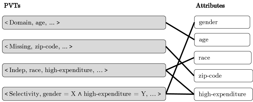
Figure 4. PVT-attribute graph. The attribute high_expenditure is associated with two discriminative PVTs. For ease of exposition, we only show profile within a PVT to denote the entire PVT.

$\mathit{People_{\mathit{pass}}}$	$\mathit{People_{fail}}$
$\langle\textsc{Domain},\mathtt{age},[22,51]\rangle$	$\langle\textsc{Domain},\mathtt{age},[20,60]\rangle$
$\langle\textsc{Missing},\mathtt{zip\_code},0.11\rangle$	$\langle\textsc{Missing},\mathtt{zip\_code},0.2\rangle$
$\langle\textsc{Indep},\mathtt{race},\mathtt{high\_expenditure},0.04\rangle$	$\langle\textsc{Indep},\mathtt{race},\mathtt{high\_expenditure},0.67\rangle$
$\langle\textsc{Selectivity},\mathtt{gender}=\text{F}$	$\langle\textsc{Selectivity},\mathtt{gender}=\text{F}$
$\wedge\mathtt{high\_expenditure}=\text{yes},0.44\rangle$	$\wedge\mathtt{high\_expenditure}=\text{yes},0.1\rangle$

Figure 5. A list of PVTs that discriminate $\mathit{People_{\mathit{pass}}}$ (Figure 3) and $\mathit{People_{fail}}$ (Figure 2) based on the scenario of Example 1 . We omit the violation and transformation functions for ease of exposition.

(Step 4) DataExposer_GRD starts intervening on $\mathit{People_{fail}}$ using the transformation of the PVT corresponding to the profile $\langle\textsc{Indep},\mathtt{race},\mathtt{high\_expenditure},0.04\rangle$ as its transformation offers the most likely fix. Then, it evaluates the malfunction of the system over the altered version of $\mathit{People_{fail}}$. Breaking the dependence between high_expenditure and race helps reduce bias in the trained classifier, and, thus, we observe a malfunction score of $0.35$ w.r.t. the altered dataset. This exposes the first explanation of malfunction.

(Step 5) DataExposer_GRD then removes the processed PVT (Indep) from the PVT-attribute graph, updates the graph according to the altered dataset, and re-iterates steps 2–4. Now the PVT corresponding to the profile Selectivity is considered for intervention as it has the highest benefit score. To do so, DataExposer_GRD over-samples tuples corresponding to female customers with $\mathtt{high\_expenditure}=yes$. This time, DataExposer_GRD intervenes on the transformed dataset obtained from the previous step. After this transformation, bias of the learned classifier further reduces and the malfunction score falls below the required threshold. Therefore, with these two interventions, DataExposer_GRD is able to expose two issues that caused undesirable behavior of the prediction model trained on $\mathit{People_{fail}}$.

(Step 6) DataExposer_GRD identifies an initial explanation over two PVTs: Indep and Selectivity. However, to verify whether it is a minimal, DataExposer_GRD tries to drop from it one PVT at a time to obtain a proper subset of the initial explanation that is also an explanation. This procedure guarantees that the explanation only consists of PVTs that are necessary, and, thus, is minimal. In this case, both Indep and Selectivity are necessary, and, thus, are part of the minimal explanation. DataExposer_GRD finally reports the following as a minimal explanation of the malfunction, where failure to satisfy the profiles is the cause and the transformations indicate fix (violation and transformation functions are omitted).

$$\{ \langle\textsc{Indep},\mathtt{race},\mathtt{high\_expenditure},0.04\rangle,$$

$$\langle\textsc{Selectivity},\mathtt{gen\-der}=\text{F}\wedge\mathtt{high\_expenditure}=\text{yes},0.44\rangle\}$$

4.2. Assumptions and Observations

We now proceed to describe our intervention algorithms more formally. We first state our assumptions and then proceed to present our observations that lead to the development of our algorithms.

Assumptions

DataExposer makes the following assumptions:

(A1) The ground-truth explanation of malfunction is captured by at least one of the discriminative PVTs. This assumption is prevalent in software-debugging literature where program predicates are assumed to be expressive enough to capture the root causes (Fariha et al., 2020; Liblit et al., 2005).

(A2) If the fix corresponds to a composition of transformations, then the malfunction score achieved after applying the composition of transformations is less than the malfunction score achieved after applying any of the constituents, and all these scores are less than the malfunction score of the original dataset. For example, consider two discriminative PVTs $X$ and $Y$ and a failing dataset $D_{\mathit{fail}}$. Our assumption is that if $\{X,Y\}$ corresponds to a minimal explanation, then $m_{S}((Y_{T}\circ X_{T})(D_{\mathit{fail}}))<m_{S}(X_{T}(D_{\mathit{fail}}))<m_{S}(D_{\mathit{fail}})$ and $m_{S}((Y_{T}\circ X_{T})(D_{\mathit{fail}}))<m_{S}(Y_{T}(D_{\mathit{fail}}))<m_{S}(D_{\mathit{fail}})$. Intuitively, this assumption states that $X$ and $Y$ have consistent (independent) effect on reducing the malfunction score, regardless of whether they are intervened together or individually. If this assumption does not hold, DataExposer can still work with additional knowledge about multiple failing and passing datasets. More details are in the appendix.

Observations

We make the following observations:

(O1) If the ground-truth explanation of malfunction corresponds to an attribute, then multiple PVTs that involve the same attribute are likely to differ across the passing and failing datasets. This observation motivates us to prioritize interventions based on PVTs that are associated with high-degree attributes in the PVT-attribute graph. Additionally, intervening on the data based on one such PVT is likely to result in an automatic “fix” of other PVTs connecting via the high-degree attribute. For example, adding noise to high_expenditure in Example 1 breaks its dependence with not only race but also with other attributes.

(O2) The PVT for which the failing dataset incurs higher violation score is more likely to be a potential explanation of malfunction.

(O3) A transformation function that affects a large number of data tuples is likely to result in a higher reduction in the malfunction score, after the transformation is applied.

PVT-attribute graph. DataExposer leverages observation O1 by constructing a bipartite graph ($G_{PA}$), called PVT-attribute graph, with all attributes $A\in\mathcal{R}(D)$ as nodes on one side and all discriminative PVTs $X\in\mathcal{X}$ on the other side. An attribute $A$ is connected to a PVT $X$ if and only if $X_{P}$ has $A$ as one of its parameters. E.g., Figure 4 shows the PVT-attribute graph w.r.t. $\mathit{People_{fail}}$ and $\mathit{People_{\mathit{pass}}}$ (Example 1). In this graph, the PVT corresponding to $\langle\textsc{Indep},\mathtt{race},\mathtt{high\_expenditure}\rangle$ is connected to two attributes, race and high_expenditure. Intuitively, this graph captures the dependence relationship between PVTs and attributes, where an intervention with respect to a PVT $X$ modifies an attribute $A$ connected to it. If this intervention reduces the malfunction score then it could possibly fix other PVTs that are connected to $A$.

Input: Failing dataset $D_{\mathit{fail}}$, passing dataset $D_{\mathit{pass}}$, malfunction score threshold $\tau$

Output: A minimal explanation set of PVTs ${\mathcal{X}^{*}}$

1

2$\mathcal{X}_{f}\leftarrow\textsc{Discover-PVT}(D_{\mathit{fail}})$

3 $\mathcal{X}_{p}\leftarrow\textsc{Discover-PVT}(D_{\mathit{pass}})$

4 $\mathcal{X}_{\cap}\leftarrow\mathcal{X}_{f}\cap\mathcal{X}_{p}$ /* Common PVTs */

5 $\mathcal{X}\leftarrow\mathcal{X}_{p}\setminus\mathcal{X}_{\cap}$ /* Discriminative PVTs */

6 $G_{PA}(V_{G},E_{G})\leftarrow\textsc{Construct-PVT-Attr-Graph}(\mathcal{X},D_{\mathit{fail}})$

7 $B\leftarrow\textsc{Calculate-Benefit-Score}(\mathcal{X},G_{PA},D_{\mathit{fail}})$

8 ${\mathcal{X}^{*}}\leftarrow\emptyset$ /* Initialize minimal explanation set to be empty */

9 $D\leftarrow D_{\mathit{fail}}$ /* Initialize dataset to the failing dataset */

10 while $m_{S}(D)>\tau$ do

11       $\mathcal{X}_{\mathtt{hda}}=\{X{\in}\mathcal{X}|(X,A){\in}E_{G}{\wedge}A{=}\operatorname{arg\,max}_{A\in\mathcal{R}(D)}deg_{G}(A)\}\!\!$ /* PVTs adjacent to high-degree attributes in $G_{PA}$ */

12       $X=\operatorname{arg\,max}_{X\in\mathcal{X}_{\mathtt{hda}}}B(X)$ /* Highest-benefit PVT */

13       $\Delta\leftarrow m_{S}(D)-m_{S}(X_{T}(D))$ /* Malfunction reduction */

14       $G_{PA}\leftarrow G_{PA}.\textsc{Remove}(X)$ /* Update $G_{PA}$ */

15       if $\Delta>0$ then /* Reduces malfunction */

16             $D\leftarrow X_{T}(D)$ /* Apply transformation */

17             $G_{PA}.\textsc{Update}(D)$ /* Update the PVT-attribute graph */

18             $B.\textsc{Update}(D)$ /* Update benefit scores */

19             ${\mathcal{X}^{*}}\leftarrow{\mathcal{X}^{*}}\cup\{X\}$ /* Add $P$ to explanation set */

20             $\mathcal{X}\leftarrow\mathcal{X}\setminus\{X\}$ /* Remove $P$ from the candidates */

21            

22      

23${\mathcal{X}^{*}}$ = Make-Minimal(${\mathcal{X}^{*}}$) /* Obtain minimality of ${\mathcal{X}^{*}}$ */

24 return ${\mathcal{X}^{*}}$ /* ${\mathcal{X}^{*}}$ is a minimal explanation */

Algorithm 1 DataExposer_GRD (greedy)

Benefit score calculation. DataExposer uses the aforementioned observations to compute a benefit score for each PVT to model their likelihood of reducing system malfunction if the corresponding transformation is used to modify the failing dataset $D_{\mathit{fail}}$. Intuitively, it assigns a high score to a PVT with a high violation score (O2) and if the corresponding transformation function modifies a large number of tuples in the dataset (O3). Formally, the benefit score of a PVT $X$ is defined as the product of violation score of $D_{\mathit{fail}}$ w.r.t. $X_{V}$ and the “coverage” of $X_{T}$. The coverage of $X_{T}$ is defined as the fraction of tuples that it modifies. Note that the benefit calculation procedure acts as a proxy of the likelihood of a PVT to offer an explanation, without actually applying any intervention.

4.3. Greedy Approach

Algorithm 1 presents the pseudocode of our greedy technique DataExposer_GRD, which takes a passing dataset $D_{\mathit{pass}}$ and a failing dataset $D_{\mathit{fail}}$ as input and returns the set of PVTs that corresponds to a minimal explanation of system malfunction.

Lines 1-1:

Identify two sets of PVTs $\mathcal{X}_{f}$ and $\mathcal{X}_{p}$ satisfied by $D_{\mathit{fail}}$ and $D_{\mathit{pass}}$, respectively.

Lines 1-1:

Discard the PVTs $\mathcal{X}_{f}\cap\mathcal{X}_{p}$ from $\mathcal{X}_{p}$ and consider the remaining discriminative ones $\mathcal{X}\equiv\mathcal{X}_{p}\setminus\mathcal{X}_{f}$ as candidates for potential explanation of system malfunction.

Line 1:

Compute the PVT-attribute graph $G_{PA}$, where the candidate PVTs $\mathcal{X}$ correspond to nodes on one side and the data attributes correspond to nodes on the other side.

Line 1:

Calculate the benefit score of each discriminative PVT $X\in\mathcal{X}$ w.r.t. $D_{\mathit{fail}}$. This procedure relies on the violation score using the violation function of the PVT and the coverage of the corresponding transformation function over $D_{\mathit{fail}}$.

Line 1-1:

Initialize the solution set $\mathcal{X}^{*}$ to $\emptyset$ and the dataset to perform intervention on $D$ to the failing dataset $\mathcal{D}_{\mathit{fail}}$. In subsequent steps, $\mathcal{X}^{*}$ will converge to a minimal explanation set and $D$ will be transformed to a dataset for which the system passes.

Line 1:

Iterate over the candidate PVTs $\mathcal{X}$ until the dataset $D$ (which is being transformed iteratively) incurs an acceptable violation score (less than the allowable threshold $\tau$).

Line 1:

Identify the subset of PVTs $\mathcal{X}_{\mathtt{hda}}\subseteq\mathcal{X}$ such that all $X\in\mathcal{X}_{\mathtt{hda}}$ are adjacent to at least one of the highest degree attributes in the current PVT-attribute graph (Observation O1).

Line 1:

Choose the PVT $X\in\mathcal{X}_{\mathtt{hda}}$ that has the maximum benefit.

Line 1:

Calculate the reduction in malfunction score if the dataset $D$ is transformed according to the transformation $X_{T}$.

Line 1:

Remove $X$ from $G_{PA}$ as it has been explored.

Lines 1-1:

If the malfunction score reduces over $X_{T}(D)$, then $X$ is added to the solution set ${\mathcal{X}^{*}}$, and $D$ is updated to $X_{T}(D)$, which is then used to update the PVT-attribute graph and benefit of each PVT. The update procedure recalculates the benefit scores of all PVTs that are connected to the attributes adjacent to $X$ in $G_{PA}$.

Line 1:

Post-process the set ${\mathcal{X}^{*}}$ to identify a minimal subset that ensure that malfunction score remains less than the threshold $\tau$. This procedure iteratively removes one PVT at a time (say $X$) from ${\mathcal{X}^{*}}$ and recalculates the malfunction score over the failing dataset $D_{\mathit{fail}}$ transformed according to the transformation functions of the PVTs in the set $\mathcal{X}^{\prime}={\mathcal{X}^{*}}\setminus\{X\}$. If the transformed dataset incurs a violation score less than $\tau$ then ${\mathcal{X}^{*}}$ is replaced with $\mathcal{X}^{\prime}$.

4.4. Group-testing-based Approach

We now present our second algorithm DataExposer_GT, which performs group interventions to identify the minimal explanation that exposes the mismatch between a dataset and a system. The group intervention methodology is applicable under the following assumption along with assumptions $A_{1}$ and $A_{2}$ (Section 4.2).

(A3) The malfunction score incurred after applying a composition of transformations is less than the malfunction score incurred by the the original dataset if and only if at least one of the constituent transformations reduces the malfunction score. For two PVTs $X$ and $Y$, $m_{S}((X_{T}\circ Y_{T})(D_{\mathit{fail}}))<m_{S}(D_{\mathit{fail}})$, iff $m_{S}(X_{T}(D_{\mathit{fail}}))<m_{S}(D_{\mathit{fail}})$ or $m_{S}(Y_{T}(D_{\mathit{fail}}))<m_{S}(D_{\mathit{fail}})$. Note that this assumption is crucial to consider group interventions and is prevalent in the group-testing literature (Du et al., 2000).

DataExposer_GT follows the classical adaptive group testing (GT) paradigm (Du et al., 2000) for interventions. To this end, it iteratively partitions the set of discriminative PVTs into two “almost” equal subsets (when the number of discriminative PVTs is odd, then the size of the two partitions will differ by one). During each iteration, all PVTs in a partition are considered for intervention together (group intervention) to evaluate the change in malfunction score. If a partition does not help reduce the malfunction score, all PVTs within that partition are discarded. While traditional GT techniques (Du et al., 2000) would use a random partitioning of the PVTs, DataExposer_GT can leverage the dependencies among PVTs (inferred from the PVT-attribute graph) to achieve more effective partitioning. Intuitively, it is beneficial to assign all PVTs whose transformations operate on the same attribute to the same partition, which is likely to enable aggressive pruning of spurious PVTs that do not reduce malfunction.

DataExposer_GRD captures the dependencies among PVTs by constructing a PVT-dependency graph $G_{PD}$. Two PVTs $U$ and $V$ are connected by an edge in $G_{PD}$ if they are connected via some attribute in $G_{PA}$. $G_{PD}$ is equivalent to $G_{PA}^{2}$ (transitive closure of $G_{PA}$), restricted to PVT nodes (excluding the attribute nodes). This ensures that PVTs that are associated via some attribute in $G_{PA}$ are connected in $G_{PD}$. DataExposer_GRD partitions $G_{PD}$ such that the number of connections (edges) between PVTs that fall in different partitions are minimized. More formally, we aim to construct two “almost” equal-sized partitions of $\mathcal{X}$ such that the number of edges between PVTs from different partitions are minimized, which maps to the problem of finding the minimum bisection of a graph (Garey et al., 1974). The minimum bisection problem is NP-hard (Garey et al., 1974) and approximate algorithms exist (Fernandes et al., 2018; Fellows et al., 2012). In this work, we use the local search algorithm (Fellows et al., 2012) (details are in the appendix).

We proceed to demonstrate the benefit of using DataExposer_GT as opposed to traditional GT with the following example.

Input: Failing dataset $D_{\mathit{fail}}$, passing dataset $D_{\mathit{pass}}$, malfunction score threshold $\tau$

Output: A minimal explanation set of PVTs ${\mathcal{X}^{*}}$

1

2$\mathcal{X}_{f}\leftarrow\textsc{Discover-PVT}(D_{\mathit{fail}})$

3 $\mathcal{X}_{p}\leftarrow\textsc{Discover-PVT}(D_{\mathit{pass}})$

4 $\mathcal{X}_{\cap}\leftarrow\mathcal{X}_{f}\cap\mathcal{X}_{p}$ /* Common PVTs */

5 $\mathcal{X}\leftarrow\mathcal{X}_{p}\setminus\mathcal{X}_{\cap}$ /* Discriminative PVTs */

6 $G_{PA}(V_{G},E_{G})\leftarrow\textsc{Construct-PVT-attr-Graph}(\mathcal{X},D_{\mathit{fail}})$

7 $D,{\mathcal{X}^{*}}\leftarrow\textsc{Group-Test}(\mathcal{X},D_{\mathit{fail}},G_{PA}^{2},\tau)$ /* Obtain an exp. */

8 ${\mathcal{X}^{*}}$ = Make-Minimal(${\mathcal{X}^{*}}$) /* Obtain minimality of ${\mathcal{X}^{*}}$ */

9 return ${\mathcal{X}^{*}}$ /* ${\mathcal{X}^{*}}$ is a minimal cause */

Algorithm 2 DataExposer_GT (group-testing-based)

Input: Candidate PVT $\mathcal{X}$, dataset $D$, PVT-dependency graph $G_{PD}$, malfunction score threshold $\tau$

Output: A transformed dataset $D^{\prime}$ and an explanation set of PVTs ${\mathcal{X}^{*}}$

1

2${\mathcal{X}^{*}}\leftarrow\emptyset$ /* Initialize explanation set to be empty */

3

4if $|\mathcal{X}|=1$ then /* Only a single PVT is candidate */

5       return $T_{\mathcal{X}}(D),\mathcal{X}$

6$\mathcal{X}^{1},\mathcal{X}^{2}\leftarrow\textsc{Get-Min-Bisection}(G_{PD},\mathcal{X})$ /* Partition $\mathcal{X}$ */

7 $\mathcal{M}\leftarrow m_{S}(D)$ /* Initial malfunction score */

8 $\Delta_{1}\leftarrow\mathcal{M}-m_{S}(\mathcal{X}^{1}_{T}(D))$ /* Malfunction reduction by $\mathcal{X}^{1}_{T}$ */

9

10if $\mathcal{M}-\Delta_{1}>\tau$ then /* ${\mathcal{X}^{1}}$ alone is insufficient */

11       $\Delta_{2}\leftarrow\mathcal{M}{-}m_{S}(\mathcal{X}^{2}_{T}(D))$ /* Malfunction reduction by $\mathcal{X}^{2}_{T}$ */

12      

13

14if $(\mathcal{M}-\Delta_{1}\leq\tau)$ OR $(\Delta_{1}>0$ AND $\mathcal{M}-\Delta_{2}>\tau)$ then

15       /* ${\mathcal{X}_{1}}$ is sufficient OR ${\mathcal{X}_{1}}$ helps AND ${\mathcal{X}_{2}}$ is insufficient */

16       $D,\mathcal{X}^{\prime}\leftarrow\textsc{Group-Test}(\mathcal{X}_{1},D,G_{PD})$

17       ${\mathcal{X}^{*}}={\mathcal{X}^{*}}\cup\mathcal{X}^{\prime}$ /* Augment explanation set */

18      if $\mathcal{M}-\Delta_{1}\leq\tau$ then /* Malfunction is acceptable */

19             return $D,{\mathcal{X}^{*}}$ /* No need to check $\mathcal{X}_{2}$ */

20      

21

22if $\Delta_{2}>0$ then /* $T_{\mathcal{X}_{2}}$ reduces malfunction */

23       $D,\mathcal{X}^{\prime}\leftarrow\textsc{Group-Test}(\mathcal{X}_{2},D,G_{PD})$

24       ${\mathcal{X}^{*}}={\mathcal{X}^{*}}\cup\mathcal{X}^{\prime}$ /* Augment explanation set */

25return $D,{\mathcal{X}^{*}}$

Algorithm 3 Group-Test

Example 1.

Consider a set of $\;8$ PVTs $\mathcal{X}=\{X_{1},\ldots,X_{8}\}$ where the ground-truth (minimal) explanation is either $\{X_{1},X_{6}\}$ or $\{X_{4},X_{8}\}$ (disjunction). An example of steps for a traditional adaptive GT approach is shown in Figure 6(c). In this case, it requires a total of $14$ interventions. Note that adaptive GT is a randomized algorithm and this example demonstrates one such execution. However, we observed similar results for other instances. In contrast to adaptive GT, DataExposer_GT constructs a min-bisection of the graph during each iteration: it does not partition $\{X_{2},X_{3}\}$ and $\{X_{5},X_{7}\}$ as none of these PVTs help reduce the malfunction. Therefore, it requires only $10$ interventions.

Algorithm 2 presents the DataExposer_GT algorithm. It starts with a set of discriminative PVTs $\mathcal{X}$ and the PVT-attribute graph $G_{PA}$. All candidate PVTs are then considered by Group-Test subroutine to identify the explanation ${\mathcal{X}^{*}}$.

Group-Test. Algorithm 3 presents the procedure that takes the set of discriminative PVTs $\mathcal{X}$, a failing dataset $D$, PVT-dependency graph $G_{PD}$, and the malfunction score threshold $\tau$ as input. It returns a transformed (fixed) dataset and an explanation.

Lines 3:

Initialize the solution set ${\mathcal{X}^{*}}$ to $\emptyset$.

Lines 3-3:

Return the candidate PVT set $\mathcal{X}$ if its cardinality is 1.

Lines 3:

Partition $\mathcal{X}$ into $\mathcal{X}_{1}$ and $\mathcal{X}_{2}$ using min-bisection of the PVT-dependency graph $G_{PD}$.

Lines 3:

Calculate the malfunction score of the input dataset.

Lines 3:

Calculate the reduction in malfunction score $\Delta_{1}$ if $D$ is intervened w.r.t. all PVTs $\mathcal{X}_{1}$.

Lines 3-3:

If the malfunction exceeds $\tau$ even after intervening on $D$ w.r.t. all PVTs in $\mathcal{X}_{1}$ then try out $\mathcal{X}_{2}$: calculate the reduction in malfunction score $\Delta_{2}$ if $D$ is intervened w.r.t. all PVTs in $\mathcal{X}_{2}$.

Lines 3-3:

Recursively call Group-Test on the partition $\mathcal{X}_{1}$ if one of the following conditions hold: (1) Intervening on $D$ w.r.t. all PVTs in $\mathcal{X}_{1}$ reduces the malfunction to be lower than $\tau$: the explanation over $\mathcal{X}_{1}$ is returned as the final explanation. (2) Intervening on $D$ w.r.t. all PVTs in $\mathcal{X}_{1}$ reduces the malfunction, but still remains above $\tau$, but intervening on $D$ w.r.t. all PVTs in $\mathcal{X}_{2}$ brings the malfunction below $\tau$: the explanation returned by the recursive call on $\mathcal{X}_{1}$ is added to the set ${\mathcal{X}^{*}}$ and $\mathcal{X}_{2}$ is processed next.

Lines 3-3:

Recursively call Group-Test on $\mathcal{X}_{2}$ if intervening on all PVTs in $\mathcal{X}_{2}$ reduces malfunction. The set of PVTs returned by this recursive call of the algorithm are added to the solution set ${\mathcal{X}^{*}}$.

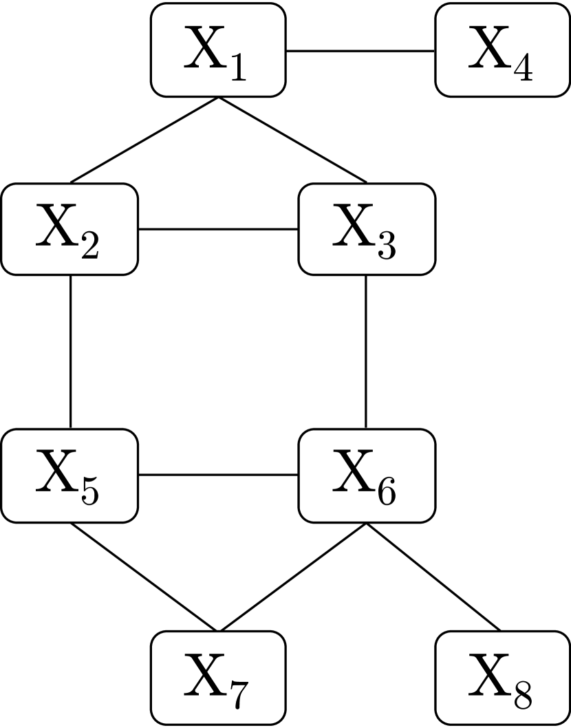
(a) Dependency graph $G_{PD}$

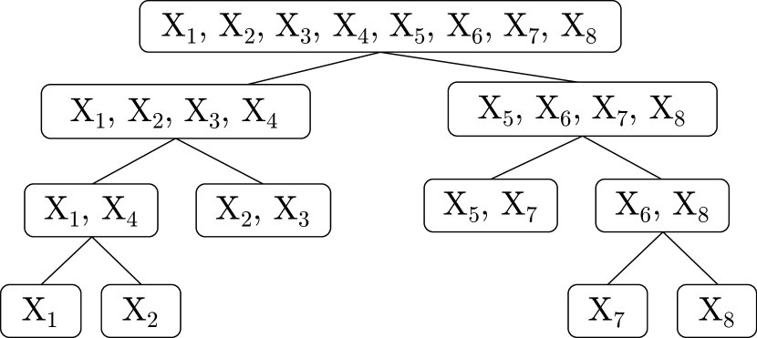
(b) Execution of DataExposer_GT

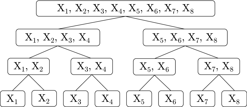
(c) Execution of traditional group testing algorithm

Figure 6. Comparison between DataExposer_GT and adaptive group testing on a toy example.

Discussion on DataExposer_GRD vs. DataExposer_GT. DataExposer_GRD intervenes by considering a single discriminative PVT at a time. Hence, in the worst case, it requires $O(|\mathcal{X}|)$ interventions where $\mathcal{X}$ denotes the set of discriminative PVTs. Note that DataExposer_GRD requires much fewer interventions in practice and would require $O(|\mathcal{X}|)$ only when any of the mentioned observations (O1–O3) do not hold. In contrast, DataExposer_GT performs group intervention by recursively partitioning the set of discriminative PVTs. Thus, the maximum number of interventions required by DataExposer_GT is $O(t\log|\mathcal{X}|)$ where $t$ denotes the number of PVTs that help reduce malfunction if the corresponding profile is altered. Note that, in expectation, DataExposer_GT requires fewer interventions than DataExposer_GRD whenever $t=o(|\mathcal{X}|/\log|\mathcal{X}|)$. DataExposer_GT is particularly helpful when multiple PVTs disjunctively explain the malfunction. However, DataExposer_GT requires an additional assumption assumption A3 (Section 4.4). We discuss the empirical impact of this assumption in Section 5.1 (Cardiovascular disease prediction). Overall, we conclude that DataExposer_GT is beneficial for applications whenever $t=O(|\mathcal{X}|/\log|\mathcal{X}|)$ and observations O1-O3 hold (more details are in the appendix).

5. Experimental Evaluation

Our experiments involving DataExposer aim to answer the following questions: (Q1) Can DataExposer correctly identify the cause and corresponding fix of mismatch between a system and a dataset for which the system fails? (Q2) How efficient is DataExposer compared to other alternative techniques? (Q3) Is DataExposer scalable with respect to the number of discriminating PVTs?

	Number of Interventions					Execution Time (seconds)
Application	DataExposerGRD	DataExposerGT	BugDoc	Anchor	GrpTest	DataExposerGRD	DataExposerGT	BugDoc	Anchor	GrpTest
Sentiment	2	3	10	303	3	25.1	23.4	64.6	4594.9	21.2
Income	1	8	20	800	10	11.8	12.5	20.0	195.5	10.4
Cardiovascular	1	NA	100	5900	NA	7.6	NA	62.1	8602.9	NA

Figure 7. Comparison of number of interventions and running time of DataExposer with other baselines. NA denotes that the technique could not identify the cause of malfunction because assumption A3 did not hold.

Baselines. Since there is no prior work on modifying a dataset according to a PVT, we adapted state-of-the-art debugging and explanation techniques to incorporate profile transformations and explain the cause of system failure. We consider three baselines: (1) BugDoc (Lourenço et al., 2020) is a recent debugging technique that explores different parameter configurations of the system to understand its behavior. We adapt BugDoc to consider each PVT as a parameter of the system and interventions as the modified configurations of the pipeline. (2) Anchor (Ribeiro et al., 2018) is a local explanation technique for classifiers that explains individual predictions based on a surrogate model. We train Anchor with PVTs as features, and the prediction variable is Pass/Fail where Pass (Fail) denotes the case where an input dataset incurs malfunction below (above) $\tau$. In this technique, each intervention creates a new data point to train the surrogate model. (3) GrpTest (Du et al., 2000) is an adaptive group testing approach that performs group interventions to expose the mismatch between the input dataset and the system. It is similar to DataExposer_GT with a difference that the recursive partitioning of PVTs is performed randomly without exploiting the PVT-dependency graph.

5.1. Real-world Case Studies

We design three case studies focusing on three different applications, where we use well-known ML models (Akbik et al., 2018; AdaBoost, fier; Random, fier) as black-box systems. For all of the three case studies, we use real-world datasets. Figure 7 presents a summary of our evaluation results.

Sentiment Prediction. The system in this study predicts sentiment of input text (reviews/tweets) and computes misclassification rate as the malfunction score. It uses flair (Akbik et al., 2018), a pre-trained classifier to predict sentiment of the input records and assumes a target attribute in the input data, indicating the ground truth sentiment: A value of $1$ for the attribute target indicates positive sentiment and a value of $-1$ indicates negative sentiment. We test the system over IMDb dataset (IMDb, aset) ($50K$ tuples) and a twitter dataset (Sentiment, aset) (around $1.6$M tuples). The malfunction score of the system on the IMDb dataset is only $0.09$ while on the twitter dataset it is $1.0$. We considered IMDb as the passing dataset and twitter as the failing dataset and used both DataExposer_GRD and DataExposer_GT to explain the mismatch between the twitter dataset and the system. The ground-truth cause of the malfunction is that the target attribute in the twitter dataset uses “4” to denote positive and “0” to denote negative sentiment (Sentiment, aset). DataExposer_GRD identifies a total of $3$ discriminative PVTs between the two datasets. One such PVT includes the profile Domain of the target attribute that has corresponding parameter $\mathbb{S}=\{-1,1\}$ for IMDb and $\mathbb{S}=\{0,4\}$ for the twitter dataset. DataExposer_GRD performs two interventions and identifies that the malfunction score reduces to $0.36$ by mapping $0\rightarrow-1$ and $4\rightarrow 1$ by intervening w.r.t. the PVT corresponding Domain, which is returned as an explanation of the malfunction.

DataExposer_GT and GrpTest both require $3$ group interventions to explain the cause of system malfunction. BugDoc and Anchor require $10$ and $303$ interventions, respectively. Anchor calculates system malfunction on datasets transformed according to various local perturbations of the PVTs in the failing dataset.

Income Prediction. The system in this study trains a Random Forest classifier (Random, fier) to predict the income of individuals while ensuring fairness towards marginalized groups. The pipeline returns the normalized disparate impact (IBM, 360) of the trained classifier w.r.t. the protected attribute (sex), as the malfunction score. Our input data includes census records (Dua and Graff, 2017) containing demographic attributes of individuals along with information about income, education, etc. We create two datasets through a random selection of records, and manually add noise to one of them to break the dependence between target and sex. The system has malfunction score of $0.195$ for the passing dataset and $0.58$ for the failing dataset due to the dependence between target and sex. DataExposer_GRD identifies a total of $43$ discriminative PVTs and constructs a PVT-attribute graph. In this graph, the target attribute has degree $15$ while all other attributes have degree $2$. The PVTs that include target are then intervened in non-increasing order of benefit. The transformation w.r.t. Indep PVT on the target attribute breaks the dependence between target and all other attributes, thereby reducing the malfunction score to $0.32$. Therefore, DataExposer_GRD requires one intervention to explain the cause of the malfunction. Our group testing algorithm DataExposer_GT and GrpTest require $8$ and $10$ interventions, respectively. Note that group testing is not very useful because the datasets contain few discriminative PVTs.

BugDoc and Anchor do not identify discriminative PVTs explicitly and consider all PVTs ($136$ for this dataset) as candidates for intervention. Anchor performs $800$ local interventions to explain the malfunction. BugDoc identifies the ground truth malfunction in $50\%$ of the runs when allowed to run fewer than $10$ interventions. It identifies the mismatch with intervention budget of $20$ but the returned solution of PVTs is not minimal. For instance, BugDoc returns two PVTs: $\{\langle$Indep, target, education$\rangle$ and $\langle$Indep, target, sex$\rangle\}$ as the explanation of malfunction.

Cardiovascular Disease Prediction. This system trains an AdaBoost classifier (AdaBoost, fier) on patients’ medical records (Cardiovascular, aset) containing age, height (in centimeters) and weight along with other attributes. It predicts if the patient has a disease and does not optimize for false positives. Therefore, the system calculates recall over the patients having cardiovascular disease, and the goal is to achieve more than $0.70$ recall. The pipeline returns the additive inverse of recall as the malfunction score. We tested the pipeline with two datasets generated through a random selection of records: (1) the passing dataset satisfies the format assumptions of the pipeline; (2) for the failing dataset we manually converted height to inches. DataExposer_GRD identifies $86$ discriminative PVTs with height, weight and age having the highest degree of $15$ in the PVT-attribute graph. Among the PVTs involving these attributes, the Domain of height has the maximum benefit, which is the ground-truth PVT too. DataExposer_GRD alters the failing dataset by applying a linear transformation and it reduces the malfunction from $0.71$ to $0.30$. This explanation matches the ground truth difference in the passing and the failing dataset. Among baselines, BugDoc and Anchor performed $100$ and $5900$ interventions, respectively. Group testing techniques are not applicable because assumption A3 (Section 4.4) does not hold. We observe that the malfunction score with a composition of transformation functions is higher than the one in the original dataset if the composition involves Indep PVT. This behavior is observed because adding noise to intervene with respect to Indep PVT worsens the classifier performance. If we remove PVTs that violate this assumption, then DataExposer_GT and GrpTest require $6$ and $9$ interventions, respectively.

Efficiency. Figure 7 presents the execution time of considered techniques for real-world applications presented above. DataExposer_GRD, DataExposer_GT and GrpTest are highly efficient and require less than $30$ seconds to explain the ground-truth cause of malfunction. In contrast, Anchor is extremely inefficient as it requires more than 143 minutes for cardiovascular, while DataExposer_GRD and BugDoc explain the malfunction within 63 seconds.

Key takeaways. Among all real-world case studies, the greedy approach DataExposer_GRD requires the fewest interventions to explain the cause of malfunction. Group testing techniques, DataExposer_GT and GrpTest, require fewer interventions than BugDoc and Anchor whenever assumption A3 (Section 4.4) holds. Anchor requires the highest number of interventions as it performs many local transformations to explain the cause of failure. BugDoc optimizes interventions by leveraging combinatorial design algorithms: it requires more interventions than DataExposer but fewer than Anchor.

5.2. Synthetic Pipelines

We evaluate the effectiveness and scalability of DataExposer_GRD and DataExposer_GT for a diverse set of synthetic scenarios.

DataExposer_GRD vs. DataExposer_GT. In this experiment, we consider a pipeline where the ground-truth explanation of malfunction violates the observations discussed in Section 4.2. Specifically, the explanation requires modifying one particular value in the dataset and its likelihood (as estimated by DataExposer_GRD) is ranked $54$ among the set of discriminative PVTs. Therefore, it requires $54$ interventions to explain the cause of malfunction. On the other hand, DataExposer_GT performs group interventions and requires only $9$ interventions. This experiment demonstrates that DataExposer_GT requires fewer interventions than DataExposer_GRD when the failing dataset and the corresponding PVTs do not satisfy the observations DataExposer_GRD relies on. We present additional experiments with complex conjunctive and disjunctive explanations of malfunction in the appendix.

Scalability. To test the scalability of our techniques, we compare their running time with increasing number of attributes and discriminative PVTs. Figure 8 shows that the time required by DataExposer_GRD and DataExposer_GT to explain the malfunction grows sub-linearly in the number of attributes and discriminative PVTs. We observe similar trend of the number of required interventions on varying these parameters. This experiment demonstrates that DataExposer_GRD requires fewer than $O(|\mathcal{X}|)$ interventions in practice (where $\mathcal{X}$ denotes the set of discriminative profiles) and validates the logarithmic dependence of DataExposer_GT on $|\mathcal{X}|$.

6. Related Work

Interventional debugging. AID (Fariha et al., 2020) uses an interventional approach to blame runtime conditions of a program for causing failure; but it is limited to software bugs and does not intervene on datasets. BugDoc (Lourenço et al., 2020) finds parameter settings in a black-box pipeline as root causes of pipeline failure; but it only reports whether a dataset is a root cause and does not explain why a dataset causes the failure. CADET (Iqbal et al., [n.d.]) uses causal inference to derive root causes of non-functional faults for hardware platforms focused on performance issues. Capuchin (Salimi et al., 2019) casts fairness in machine learning as a database repair problem and adds or removes rows in the training data to simulate a fair world; but it does not aim to find cause of unfairness.

Data explanation. Explanations for query results have been abundantly studied (Wang et al., 2015; Bailis et al., 2017; Chirigati et al., 2016; El Gebaly et al., 2014). Some works find causes of errors in data generation processes (Wang et al., 2015), while others discover relationships among attributes (Bailis et al., 2017; El Gebaly et al., 2014), and across datasets (Chirigati et al., 2016). ExceLint (Barowy et al., 2018) exploits the spatial structure of spreadsheets to look for erroneous formulas. Unlikely interventional efforts, these approaches operate on observational data, and do not generate additional test cases.

Model explanation. Machine learning interpreters (Ribeiro et al., 2016, 2018) perturb testing data to learn a surrogate for models. Their goal is not to find mismatch between data and models. Debugging methods for ML pipelines are similar to data explanation (Cadamuro et al., 2016; Breck et al., 2019), where training data may cause model’s underperformance. (Varma et al., 2017) and (Kulesza et al., 2015) discuss principled ways to find reasons of malfunctions. Wu et al. (Wu et al., 2020) allow users to complain about outputs of SQL queries, and presents data points whose removal resolves the complaints. (Schelter et al., 2020) validates when models fail on certain datasets and assumes knowledge of the mechanism that corrupts the data. We aim to find discriminative profiles among datasets without such knowledge.

Causal inference debugging. Data-driven approaches have been taken for causal-inference-based fault localization (Gulzar et al., 2018; Attariyan and Flinn, 2011; Attariyan et al., 2012; Chen et al., 2002), software testing (Fraser and Arcuri, 2013; Godefroid et al., 2008; Holler et al., 2012; Johnson et al., 2020; Zeller, 1999), and statistical debugging (Zheng et al., 2006; Liblit et al., 2005). However, they use a white-box strategy or are application-specific. Causal relational learning (Salimi et al., 2020) infers causal relationships in relational data, but it does not seek mismatches between the data and the systems. Our work shares similarity with BugEx (Rößler et al., 2012), which generates test cases to isolate root causes. However, it assumes complete knowledge of the program, and data-flow paths.

Data debugging. Porting concepts of debugging from software to data has gained attention in data management community (Muşlu et al., 2013; Brachmann et al., 2019). Dagger (Rezig et al., 2020b, a) provides data debugging primitives for white-box interactions with data-driven pipelines. CheckCell (Barowy et al., 2014) ranks data cells that unusually affect output of a given target. However, it is not meant for large datasets where single cells are unlikely to causes malfunction. Moreover, CheckCell cannot expose combination of root causes. DataExposer is general-purpose, application-agnostic, and interventional, providing causally verified issues mismatch between the data and the systems.

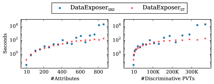
Figure 8. Execution time of DataExposer_GRD vs. DataExposer_GT with varying number of data attributes (left) and discriminative PVTs (right) over synthetic pipelines.

7. Summary and Future Directions

We introduced the problem of identifying causes and fixes of mismatch between data and systems that operate on data. To this end, we presented DataExposer, a framework that reports violation of data profiles as causally verified root causes of system malfunction and reports fixes in the form of transformation functions. We demonstrated the effectiveness and efficacy of DataExposer in explaining the reason of mismatch in several real-world and synthetic data-driven pipelines, significantly outperforming the state of the art. In future, we want to extend DataExposer to support more complex classes of data profiles. Additionally, we plan to investigate ways that can facilitate automatic repair of both data and the system guided by the identified data issues.

Appendix A Minimum Bisection

Algorithm 4 presents the local search algorithm (Fellows et al., 2012) that DataExposer_GT uses to partition the set of discriminative PVTs. It is an anytime algorithm (Zilberstein, 1996) and is known to be very efficient in most practical settings (Fellows et al., 2012).

Line 4:

Initialize the solution $\mathcal{X}_{1},\mathcal{X}_{2}$ to a randomized partition of $\mathcal{X}$ where $|\mathcal{X}_{1}|-|\mathcal{X}_{2}|\leq 1$.

Lines 2-4:

Iteratively try to improve the solution by performing local search.

Line 4:

Count the number of cut edges, i.e., edges that connect two nodes from different partitions.

Line 4:

Initialize the number of cut edges in an improved partitioning to be equal to the current number of cut edges.

Lines 4-4:

Swap a pair of PVTs between the partitions to create two temporary partitions.

Lines 4:

Count the number of cut edges between the temporary partitions.

Lines 4-4:

If swapping the PVT pairs reduces the number of cut edges, then update the partitions and terminate the current iteration.

Line 4:

Stop searching for an improved partitioning reduction in the number of cut edges is no longer possible.

Line 4:

Return the updated partitions $\mathcal{X}_{1},\mathcal{X}_{2}$ as the solution.

Appendix B Modeling Interaction among PVT Interventions

We now extend our techniques for the setting when intervening on one PVT may affect the impact of intervention on another PVT. For example, when altering the failing dataset with respect to PVT $P_{1}$ does not help reduce malfunction when considered in isolation, but, malfunction reduces when the failing dataset is intervened with respect to PVT $P_{1}$ along with another PVT $P_{2}$. In such a setting, assumption A2 does not hold and DataExposer may fail to identify the ground-truth cause of malfunction.

To address this issue, we propose to leverage multiple passing and failing datasets. Using this additional knowledge, we generate a decision tree to guide DataExposer. The key idea is to fit a decision tree based on the PVTs and the relative decrease of the malfunction score ($m_{S}{D}$) with respect to the maximum allowable malfunction score threshold ($\tau$). Each training data point for learning the decision tree consists of the set of PVTs $\mathcal{X}_{i}$, extracted from dataset $D_{i}$, and the outcome is the Boolean assessment of whether $m_{S}(D_{i})\leq\tau$. Each path of the tree can be seen as a conjunction of PVTs. If a conjunction leads to a consistent outcome (a “pure” leaf), then that combination becomes an explanation “candidate”. The candidates are then verified by Algorithm 5, where we perform interventions on an arbitrary failing dataset.

Line 5:

Traverse the decision tree at least once.

Line 5-5:

Follow the decision-tree paths until we find a conjunction of PVTs $\mathcal{X}$ that reduces the malfunction score of $D_{\mathit{fail}}$ so that $m_{S}(D_{\mathit{fail}})\leq\tau$. If no candidate conjunction of PVTs can convert $D_{\mathit{fail}}$ to a passing dataset, then rebuild the decision tree.

Input: Dependency Graph $G_{PD}$, discriminative PVTs $\mathcal{X}$

Output: Partitions $\mathcal{X}_{1}$, $\mathcal{X}_{2}$

1 $\mathcal{X}_{1},\mathcal{X}_{2}\leftarrow\textsc{Random-Bisection}(\mathcal{X})$ /* Initialization */

2 do

3       $C\leftarrow\sum\limits_{X_{1}\in\mathcal{X}_{1},X_{2}\in\mathcal{X}_{2}}\mathbbm{1}_{G_{PD}}(X_{1},X_{2})$ /* #Cut edges */

4       $C^{\prime}\leftarrow C$ /* Initialize */

5       foreach $X_{1}\in\mathcal{X}_{1}$ do

6             foreach $X_{2}\in\mathcal{X}_{2}$ do

7                   $\mathcal{X}_{1}^{\prime}\leftarrow\mathcal{X}_{1}\cup\{X_{2}\}\setminus\{X_{1}\}$ /* Swap PVTs */

8                   $\mathcal{X}_{2}^{\prime}\leftarrow\mathcal{X}_{2}\cup\{X_{1}\}\setminus\{X_{2}\}$ /* Swap PVTs */

9                   $C^{\prime}\leftarrow\sum\limits_{X_{1}\in\mathcal{X}_{1}^{\prime},X_{2}\in\mathcal{X}_{2}^{\prime}}\mathbbm{1}_{G_{PD}}(X_{1},X_{2})$ /* #Cut edges */

10                   if $C^{\prime}<C$ then /* Cut size is reduced */

11                         $\mathcal{X}_{1}\leftarrow\mathcal{X}_{1}^{\prime}$ /* Update partition */

12                         $\mathcal{X}_{2}\leftarrow\mathcal{X}_{2}^{\prime}$ /* Update partition */

13                         break

14                  

15            

16      

17while $C^{\prime}<C$; /* As long as cut size reduces */

return $\mathcal{X}_{1},\mathcal{X}_{2}$ /* $\mathcal{X}_{1},\mathcal{X}_{2}$ are returned as the solution */

Algorithm 4 Get-Min-Bisection

Line 5:

Find the paths $\Pi$ of the decision tree that lead to pure leaves (malfunction score is less than $\tau$ whenever all PVTs in the paths, in conjunction, are observed) and sort them by their PVTs’ benefit scores, as defined in Algorithm 1.

Line 5:

Record that some candidate PVTs were computed.

Lines 5-5:

Iteratively test each conjunction of PVTs $\mathcal{X}$.

Line 5:

Transform the failing dataset $D_{\mathit{fail}}$ w.r.t $\mathcal{X}$ to obtain $D_{t}$.

Lines 5-5:

If the transformed dataset $D_{t}$ reduces the malfunction score, then return $\mathcal{X}$ as a cause of malfunction. Otherwise, add a new instance (data point) to re-train the decision tree and recompute $\Pi$.

In future work, we plan to extend this approach to leverage combinatorial-design-based techniques to efficiently intervene PVTs to initialize the decision tree algorithm (Colbourn et al., 2006).

Appendix C Discussion on DataExposer_GRD vs. DataExposer_GT

As discussed in Section 4.4, DataExposer_GRD always identifies the ground-truth cause of malfunction, but, the number of interventions required may increase if observations O1-O3 do not hold. If O1 does not hold, then the initial ordering of attributes, which is computed based on their degree in PVT-Attribute graph $G_{PA}$, may not be accurate. In this case, DataExposer_GRD may require $O(\mathcal{X})$ interventions to explain the cause of system malfunction. Similarly, whenever O2 or O3 fail, the benefit-based ordering of the PVTs is likely to be incorrect. In applications where O1 holds but O2 and O3 do not hold, $G_{PA}$ is expected to be accurate and the number of required interventions is $O(r)$, where $r$ is the degree of the attribute that has the highest degree in $G_{PA}$. In contrast, DataExposer_GT requires $O(t\log|\mathcal{X}|)$ interventions even when these observations are violated. Therefore, DataExposer_GRD is beneficial whenever all of these observations hold, or $t=\Omega(|\mathcal{X}|/\log|\mathcal{X}|)$.

Input: Failing dataset $D_{\mathit{fail}}$, decision tree $DT$, malfunction score threshold $\tau$

1 $\textsc{Update-Paths}\leftarrow\texttt{true}$ /* Indicates whether to explore decision tree paths */

2 while Update-Paths do

3       Let $\Pi$ be the set of paths in $DT$ that are observed for instances where system malfunction score is less than $\tau$. All PVTs along a path are considered in conjunction and sorted by decreasing order of their benefit score.

4      

5      $\textsc{Update-Paths}\leftarrow\texttt{false}$ /* $\Pi$ is up-to-date */

6      

7      for $\mathcal{X}\in\Pi$ do

8             $D_{t}\leftarrow\mathcal{X}_{T}(D_{\mathit{fail}})$ /* Transform $D_{\mathit{fail}}$ wrt $\mathcal{X}$ */

9            

10            if $m_{S}(D_{t})\leq\tau$ then /* Cause has been identified */

11                   return $\mathcal{X}$

12            else

13                   $DT.\textsc{Update}(D_{t},\texttt{Fail})$ /* Add instance to tree */

14                  

15                  $\textsc{Update-Paths}\leftarrow\texttt{true}$ /* Recompute $\Pi$ */

16                  

17            

18      

return $\emptyset$

Algorithm 5 Greedy + Decision Tree Approach

Appendix D Effect of Various Parameters

In this experiment, we test the effect of the number of dataset attributes and the number of discriminative PVTs on the efficacy of DataExposer algorithms, and contrast those with other state-of-the-art baselines. We also investigate the influence of the number of PVTs involved in the root causes and their interactions on the number of interventions each method requires.

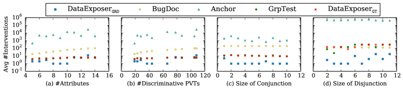
Figure 9. Average number of interventions required by two versions of DataExposer and three other techniques for varying number of attributes, discriminative PVTs, size of single conjunctive root causes, and size of disjunctive root causes.

D.1. Effect of Number of Attributes and PVTs

Figure 9(a) presents the effect of changing the number of attributes in the datasets on the number of required interventions. DataExposer_GRD requires fewer than $5$ interventions on average. In contrast, BugDoc and Anchor require orders of magnitude more interventions. The number of interventions required by BugDoc grows linearly with the number of attributes. At the same time, Anchor perturbs all PVTs to solve a multi-armed bandit problem: the more PVTs affect the pipeline errors, the more interventions are needed. Group-testing-based approaches also require more intervention than that of DataExposer_GRD, and grow logarithmically with the number of data attributes.

Figure 9(b) depicts the effect of the number of discriminative PVTs on the number of required interventions. DataExposer_GRD shows superior performance as it requires fewer than $10$ interventions even when the number of discriminative PVTs go beyond $100$. Here, we observe trends similar the one in Figure 9(a) for other baselines as the number of PVTs are strongly and positively correlated to the number attributes.

D.2. Effect of Number of Root Causes and their Interactions

The pipelines presented in Figures 9(a) and 9(b) have a single PVT as the root cause of the malfunction. In Figure 9(c), we fix the number of attributes to $15$ and the number of discriminative PVTs between the passing and the failing datasets to $136$. We also define the root cause to be a conjunction over a set of PVTs of varying cardinalities. We find that the cardinality of the root-cause set (length of the conjunctive cause) does not impact the number of interventions as much as the number of attributes and the number of discriminative PVTs do. However, having more than one cause for malfunction (i.e., a disjunctive cause) requires more interventions for Anchor and the Group-Test techniques, as shown in Figure 9(d). DataExposer_GRD still needs orders of magnitude fewer interventions than these other approaches, although the probability of failing to find any feasible transformation, which decreases malfunctions scores, increases with the number of possible root causes within the disjunction.

References

- (1)
- AdaBoost (fier) AdaBoost Classifier. https://scikit-learn.org/stable/modules/generated/sklearn.ensemble.AdaBoostClassifier.html
- Akbik et al. (2018) Alan Akbik, Duncan Blythe, and Roland Vollgraf. 2018. Contextual String Embeddings for Sequence Labeling. In COLING 2018, 27th International Conference on Computational Linguistics. 1638–1649.
- Attariyan et al. (2012) Mona Attariyan, Michael Chow, and Jason Flinn. 2012. X-Ray: Automating Root-Cause Diagnosis of Performance Anomalies in Production Software. In Proceedings of USENIX OSDI (Hollywood, CA, USA) (OSDI’12). USENIX Association, USA, 307–320.
- Attariyan and Flinn (2011) Mona Attariyan and Jason Flinn. 2011. Automating Configuration Troubleshooting with ConfAid. ;login: 36, 1 (2011), 1–14.
- Bailis et al. (2017) Peter Bailis, Edward Gan, Samuel Madden, Deepak Narayanan, Kexin Rong, and Sahaana Suri. 2017. MacroBase: Prioritizing Attention in Fast Data. In Proceedings of the 2017 ACM International Conference on Management of Data (Chicago, Illinois, USA) (SIGMOD ’17). ACM, New York, NY, USA, 541–556. https://doi.org/10.1145/3035918.3035928
- Barowy et al. (2018) Daniel W Barowy, Emery D Berger, and Benjamin Zorn. 2018. ExceLint: Automatically finding spreadsheet formula errors. Proceedings of the ACM on Programming Languages 2, OOPSLA (2018), 1–26.
- Barowy et al. (2014) Daniel W. Barowy, Dimitar Gochev, and Emery D. Berger. 2014. CheckCell: data debugging for spreadsheets. In OOPSLA. 507–523. https://doi.org/10.1145/2660193.2660207
- Bellamy et al. (2018) Rachel KE Bellamy, Kuntal Dey, Michael Hind, Samuel C Hoffman, Stephanie Houde, Kalapriya Kannan, Pranay Lohia, Jacquelyn Martino, Sameep Mehta, Aleksandra Mojsilovic, et al. 2018. AI Fairness 360: An extensible toolkit for detecting, understanding, and mitigating unwanted algorithmic bias. arXiv preprint arXiv:1810.01943 (2018).
- Bias (ring) Bias in Amazon Hiring. https://becominghuman.ai/amazons-sexist-ai-recruiting-tool-how-did-it-go-so-wrong-e3d14816d98e
- Brachmann et al. (2019) Mike Brachmann, Carlos Bautista, Sonia Castelo, Su Feng, Juliana Freire, Boris Glavic, Oliver Kennedy, Heiko Müeller, Rémi Rampin, William Spoth, et al. 2019. Data debugging and exploration with vizier. In Proceedings of the 2019 International Conference on Management of Data. 1877–1880.
- Breck et al. (2019) Eric Breck, Neoklis Polyzotis, Sudip Roy, Steven Euijong Whang, and Martin Zinkevich. 2019. Data validation for machine learning. In Conference on Systems and Machine Learning (SysML). https://www. sysml. cc/doc/2019/167. pdf.
- Cadamuro et al. (2016) Gabriel Cadamuro, Ran Gilad-Bachrach, and Xiaojin Zhu. 2016. Debugging machine learning models. In ICML Workshop on Reliable Machine Learning in the Wild.
- Cardiovascular (aset) Cardiovascular Disease dataset. https://www.kaggle.com/sulianova/cardiovascular-disease-dataset
- Caruccio et al. (2016) Loredana Caruccio, Vincenzo Deufemia, and Giuseppe Polese. 2016. On the discovery of relaxed functional dependencies. In Proceedings of the 20th International Database Engineering & Applications Symposium. 53–61.
- Casalicchio et al. (2018) Giuseppe Casalicchio, Christoph Molnar, and Bernd Bischl. 2018. Visualizing the feature importance for black box models. In Joint European Conference on Machine Learning and Knowledge Discovery in Databases. Springer, 655–670.
- Chen et al. (2002) Mike Y. Chen, Emre Kiciman, Eugene Fratkin, Armando Fox, and Eric Brewer. 2002. Pinpoint: Problem Determination in Large, Dynamic Internet Services. In Proceedings of IEEE DSN (DSN’02). IEEE, USA, 595–604.
- Chirigati et al. (2016) Fernando Chirigati, Harish Doraiswamy, Theodoros Damoulas, and Juliana Freire. 2016. Data Polygamy: The Many-Many Relationships Among Urban Spatio-Temporal Data Sets. In Proceedings of ACM SIGMOD (San Francisco, California, USA) (SIGMOD ’16). ACM, New York, NY, USA, 1011–1025. https://doi.org/10.1145/2882903.2915245
- Chu et al. (2013) Xu Chu, Ihab F. Ilyas, and Paolo Papotti. 2013. Discovering Denial Constraints. PVLDB 6, 13 (2013), 1498–1509. https://doi.org/10.14778/2536258.2536262
- Colbourn et al. (2006) Charles J. Colbourn, Sosina S. Martirosyan, Gary L. Mullen, Dennis Shasha, George B. Sherwood, and Joseph L. Yucas. 2006. Products of mixed covering arrays of strength two. Journal of Combinatorial Designs 2 (2006), 124–138.
- Dong et al. (2014) Xin Luna Dong, Evgeniy Gabrilovich, Geremy Heitz, Wilko Horn, Kevin Murphy, Shaohua Sun, and Wei Zhang. 2014. From Data Fusion to Knowledge Fusion. Proc. VLDB Endow. 7, 10 (2014), 881–892. https://doi.org/10.14778/2732951.2732962
- Du et al. (2000) Dingzhu Du, Frank K Hwang, and Frank Hwang. 2000. Combinatorial group testing and its applications. Vol. 12. World Scientific.
- Dua and Graff (2017) Dheeru Dua and Casey Graff. 2017. UCI Machine Learning Repository. http://archive.ics.uci.edu/ml
- El Gebaly et al. (2014) Kareem El Gebaly, Parag Agrawal, Lukasz Golab, Flip Korn, and Divesh Srivastava. 2014. Interpretable and Informative Explanations of Outcomes. Proceedings of VLDB Endowment 8, 1 (Sept. 2014), 61–72. https://doi.org/10.14778/2735461.2735467
- Fan et al. (2009) Wenfei Fan, Floris Geerts, Laks V. S. Lakshmanan, and Ming Xiong. 2009. Discovering Conditional Functional Dependencies. In Proceedings of the 25th International Conference on Data Engineering, ICDE 2009, March 29 2009 - April 2 2009, Shanghai, China. 1231–1234. https://doi.org/10.1109/ICDE.2009.208
- Fariha et al. (2020) Anna Fariha, Suman Nath, and Alexandra Meliou. 2020. Causality-Guided Adaptive Interventional Debugging. In SIGMOD. 431–446. https://doi.org/10.1145/3318464.3389694
- Fariha et al. (2021) Anna Fariha, Ashish Tiwari, Arjun Radhakrishna, Sumit Gulwani, and Alexandra Meliou. 2021. Conformance Constraint Discovery: Measuring Trust in Data-Driven Systems. In SIGMOD. https://doi.org/10.1145/3448016.3452795
- Fellows et al. (2012) Michael R Fellows, Fedor V Fomin, Daniel Lokshtanov, Frances Rosamond, Saket Saurabh, and Yngve Villanger. 2012. Local search: Is brute-force avoidable? J. Comput. System Sci. 78, 3 (2012), 707–719.
- Fernandes et al. (2018) Cristina G Fernandes, Tina Janne Schmidt, and Anusch Taraz. 2018. On minimum bisection and related cut problems in trees and tree-like graphs. Journal of Graph Theory 89, 2 (2018), 214–245.
- Fraser and Arcuri (2013) Gordon Fraser and Andrea Arcuri. 2013. Whole test suite generation. IEEE Transactions on Software Engineering 39, 2 (2013), 276–291.
- Galhotra et al. (2019) Sainyam Galhotra, Udayan Khurana, Oktie Hassanzadeh, Kavitha Srinivas, Horst Samulowitz, and Miao Qi. 2019. Automated Feature Enhancement for Predictive Modeling using External Knowledge. In 2019 International Conference on Data Mining Workshops (ICDMW). IEEE, 1094–1097.
- Garey et al. (1974) Michael R Garey, David S Johnson, and Larry Stockmeyer. 1974. Some simplified NP-complete problems. In Proceedings of the sixth annual ACM symposium on Theory of computing. 47–63.
- Godefroid et al. (2008) Patrice Godefroid, Michael Y. Levin, and David A. Molnar. 2008. Automated whitebox fuzz testing. In Proceedings of NDSS. 151–166.
- Google (cism) Google Vision Racism. https://algorithmwatch.org/en/story/google-vision-racism/
- Gulzar et al. (2018) Muhammad Ali Gulzar, Siman Wang, and Miryung Kim. 2018. BigSift: Automated Debugging of Big Data Analytics in Data-Intensive Scalable Computing. In Proceedings of ESEC/FSE (Lake Buena Vista, FL, USA) (ESEC/FSE 2018). ACM, New York, NY, USA, 863–866. https://doi.org/10.1145/3236024.3264586
- Hailpern and Santhanam (2002) Brent Hailpern and Padmanabhan Santhanam. 2002. Software debugging, testing, and verification. IBM Systems Journal 41, 1 (2002), 4–12.
- Hellerstein (2008) Joseph M Hellerstein. 2008. Quantitative Data Cleaning for Large Databases. (2008).
- Henzinger et al. (2003) Thomas A Henzinger, Ranjit Jhala, Rupak Majumdar, and Grégoire Sutre. 2003. Software verification with BLAST. In International SPIN Workshop on Model Checking of Software. Springer, 235–239.
- Holler et al. (2012) Christian Holler, Kim Herzig, and Andreas Zeller. 2012. Fuzzing with code fragments. In Proceedings of USENIX Security Symposium. 445–458.
- IBM ( 360) IBM AIF 360. https://aif360.mybluemix.net/
- Ilyas et al. (2004) Ihab F Ilyas, Volker Markl, Peter Haas, Paul Brown, and Ashraf Aboulnaga. 2004. CORDS: automatic discovery of correlations and soft functional dependencies. In Proceedings of the 2004 ACM SIGMOD international conference on Management of data. 647–658.
- IMDb (aset) IMDb Dataset. https://www.kaggle.com/lakshmi25npathi/imdb-dataset-of-50k-movie-reviews
- Iqbal et al. ([n.d.]) Md Shahriar Iqbal, Rahul Krishna, Mohammad Ali Javidian, Baishakhi Ray, and Pooyan Jamshidi. [n.d.]. CADET: A Systematic Method For Debugging Misconfigurations using Counterfactual Reasoning. ([n. d.]).
- Is Amazon same-day delivery service racist? (2016) Is Amazon same-day delivery service racist? 2016. The Christian Science Monitor. https://www.csmonitor.com/Business/2016/0423/Is-Amazon-same-day-delivery-service-racist
- Johnson et al. (2020) Brittany Johnson, Yuriy Brun, and Alexandra Meliou. 2020. Causal Testing: Finding Defects’ Root Causes. In ICSE.
- Koudas et al. (2009) Nick Koudas, Avishek Saha, Divesh Srivastava, and Suresh Venkatasubramanian. 2009. Metric functional dependencies. In 2009 IEEE 25th International Conference on Data Engineering. IEEE, 1275–1278.
- Kulesza et al. (2015) Todd Kulesza, Margaret Burnett, Weng-Keen Wong, and Simone Stumpf. 2015. Principles of explanatory debugging to personalize interactive machine learning. In Proceedings of the 20th international conference on intelligent user interfaces. 126–137.
- Kumar et al. (2013) Amresh Kumar, M Kiran, and BR Prathap. 2013. Verification and validation of mapreduce program model for parallel k-means algorithm on hadoop cluster. In 2013 Fourth International Conference on Computing, Communications and Networking Technologies (ICCCNT). IEEE, 1–8.
- Langer and Naumann (2016) Philipp Langer and Felix Naumann. 2016. Efficient order dependency detection. VLDB J. 25, 2 (2016), 223–241. https://doi.org/10.1007/s00778-015-0412-3
- Liblit et al. (2005) Ben Liblit, Mayur Naik, Alice X Zheng, Alex Aiken, and Michael I Jordan. 2005. Scalable statistical bug isolation. Acm Sigplan Notices 40, 6 (2005), 15–26.
- Liu et al. (2019) Haopeng Liu, Shan Lu, Madan Musuvathi, and Suman Nath. 2019. What bugs cause production cloud incidents?. In Proceedings of the Workshop on Hot Topics in Operating Systems, HotOS 2019, Bertinoro, Italy, May 13-15, 2019. 155–162. https://doi.org/10.1145/3317550.3321438
- Lourenço et al. (2020) Raoni Lourenço, Juliana Freire, and Dennis E. Shasha. 2020. BugDoc: Algorithms to Debug Computational Processes. In SIGMOD. 463–478. https://doi.org/10.1145/3318464.3389763
- Mesbah et al. (2011) Ali Mesbah, Arie Van Deursen, and Danny Roest. 2011. Invariant-based automatic testing of modern web applications. IEEE Transactions on Software Engineering 38, 1 (2011), 35–53.
- Muşlu et al. (2013) Kıvanç Muşlu, Yuriy Brun, and Alexandra Meliou. 2013. Data debugging with continuous testing. In Proceedings of the 2013 9th Joint Meeting on Foundations of Software Engineering. 631–634.
- Papenbrock et al. (2015a) Thorsten Papenbrock, Jens Ehrlich, Jannik Marten, Tommy Neubert, Jan-Peer Rudolph, Martin Schönberg, Jakob Zwiener, and Felix Naumann. 2015a. Functional dependency discovery: An experimental evaluation of seven algorithms. Proceedings of the VLDB Endowment 8, 10 (2015), 1082–1093.
- Papenbrock et al. (2015b) Thorsten Papenbrock, Sebastian Kruse, Jorge-Arnulfo Quiané-Ruiz, and Felix Naumann. 2015b. Divide & conquer-based inclusion dependency discovery. Proceedings of the VLDB Endowment 8, 7 (2015), 774–785.
- Python (kage) Python Rexpy package. {https://tdda.readthedocs.io/en/v1.0.30/rexpy.html}
- Random (fier) Random Forest Classifier. {https://scikit-learn.org/stable/modules/generated/sklearn.ensemble.RandomForestClassifier.html}
- Rawal et al. (2020) Kaivalya Rawal, Ece Kamar, and Himabindu Lakkaraju. 2020. Can I Still Trust You?: Understanding the Impact of Distribution Shifts on Algorithmic Recourses. arXiv preprint arXiv:2012.11788 (2020).
- Rezig et al. (2020a) El Kindi Rezig, Ashrita Brahmaroutu, Nesime Tatbul, Mourad Ouzzani, Nan Tang, Timothy G. Mattson, Samuel Madden, and Michael Stonebraker. 2020a. Debugging Large-Scale Data Science Pipelines using Dagger. Proc. VLDB Endow. 13, 12 (2020), 2993–2996. http://www.vldb.org/pvldb/vol13/p2993-rezig.pdf
- Rezig et al. (2020b) El Kindi Rezig, Lei Cao, Giovanni Simonini, Maxime Schoemans, Samuel Madden, Nan Tang, Mourad Ouzzani, and Michael Stonebraker. 2020b. Dagger: A Data (not code) Debugger. In CIDR 2020, 10th Conference on Innovative Data Systems Research, Amsterdam, The Netherlands, January 12-15, 2020, Online Proceedings. http://cidrdb.org/cidr2020/papers/p35-rezig-cidr20.pdf
- Ribeiro et al. (2016) Marco Tulio Ribeiro, Sameer Singh, and Carlos Guestrin. 2016. ”Why should I trust you?” Explaining the predictions of any classifier. In Proceedings of the 22nd ACM SIGKDD international conference on knowledge discovery and data mining. 1135–1144.
- Ribeiro et al. (2018) Marco Tulio Ribeiro, Sameer Singh, and Carlos Guestrin. 2018. Anchors: High-Precision Model-Agnostic Explanations.. In AAAI, Vol. 18. 1527–1535.
- Rößler et al. (2012) Jeremias Rößler, Gordon Fraser, Andreas Zeller, and Alessandro Orso. 2012. Isolating failure causes through test case generation. In International Symposium on Software Testing and Analysis, ISSTA 2012, Minneapolis, MN, USA, July 15-20, 2012, Mats Per Erik Heimdahl and Zhendong Su (Eds.). ACM, 309–319. https://doi.org/10.1145/2338965.2336790
- Salimi et al. (2020) Babak Salimi, Harsh Parikh, Moe Kayali, Lise Getoor, Sudeepa Roy, and Dan Suciu. 2020. Causal Relational Learning. In Proceedings of the 2020 International Conference on Management of Data, SIGMOD Conference 2020, online conference [Portland, OR, USA], June 14-19, 2020. 241–256. https://doi.org/10.1145/3318464.3389759
- Salimi et al. (2019) Babak Salimi, Luke Rodriguez, Bill Howe, and Dan Suciu. 2019. Interventional Fairness: Causal Database Repair for Algorithmic Fairness. In SIGMOD. 793–810. https://doi.org/10.1145/3299869.3319901
- Scheines et al. (1998) Richard Scheines, Peter Spirtes, Clark Glymour, Christopher Meek, and Thomas Richardson. 1998. The TETRAD project: Constraint based aids to causal model specification. Multivariate Behavioral Research 33, 1 (1998), 65–117.
- Schelter et al. (2020) Sebastian Schelter, Tammo Rukat, and Felix Bießmann. 2020. Learning to Validate the Predictions of Black Box Classifiers on Unseen Data. In SIGMOD. 1289–1299. https://doi.org/10.1145/3318464.3380604
- Sentiment (aset) Sentiment 140 dataset. https://www.kaggle.com/kazanova/sentiment140
- Song and Chen (2011) Shaoxu Song and Lei Chen. 2011. Differential dependencies: Reasoning and discovery. ACM Transactions on Database Systems (TODS) 36, 3 (2011), 1–41.
- Varma et al. (2017) Paroma Varma, Dan Iter, Christopher De Sa, and Christopher Ré. 2017. Flipper: A systematic approach to debugging training sets. In Proceedings of the 2nd Workshop on Human-in-the-Loop Data Analytics. 1–5.
- Wang et al. (2015) Xiaolan Wang, Xin Luna Dong, and Alexandra Meliou. 2015. Data X-Ray: A Diagnostic Tool for Data Errors. In Proceedings of the 2015 ACM SIGMOD International Conference on Management of Data, Melbourne, Victoria, Australia, May 31 - June 4, 2015. 1231–1245. https://doi.org/10.1145/2723372.2750549
- Wu et al. (2020) Weiyuan Wu, Lampros Flokas, Eugene Wu, and Jiannan Wang. 2020. Complaint-driven Training Data Debugging for Query 2.0. In Proceedings of the 2020 ACM SIGMOD International Conference on Management of Data. 1317–1334.
- Yan et al. (2020) Jing Nathan Yan, Oliver Schulte, Mohan Zhang, Jiannan Wang, and Reynold Cheng. 2020. SCODED: Statistical Constraint Oriented Data Error Detection. In Proceedings of the 2020 International Conference on Management of Data, SIGMOD Conference 2020, online conference [Portland, OR, USA], June 14-19, 2020. 845–860. https://doi.org/10.1145/3318464.3380568
- Zeller (1999) Andreas Zeller. 1999. Yesterday, My Program Worked. Today, It Does Not. Why?. In Software Engineering - ESEC/FSE’99, 7th European Software Engineering Conference, Held Jointly with the 7th ACM SIGSOFT Symposium on the Foundations of Software Engineering, Toulouse, France, September 1999, Proceedings. 253–267. https://doi.org/10.1007/3-540-48166-4_16
- Zheng et al. (2006) Alice X. Zheng, Michael I. Jordan, Ben Liblit, Mayur Naik, and Alex Aiken. 2006. Statistical Debugging: Simultaneous Identification of Multiple Bugs. In Proceedings of ICML (Pittsburgh, Pennsylvania, USA) (ICML’06). ACM, New York, NY, USA, 1105–1112. https://doi.org/10.1145/1143844.1143983
- Zilberstein (1996) Shlomo Zilberstein. 1996. Using anytime algorithms in intelligent systems. AI magazine 17, 3, 73–73.