VPP-ART: An Efficient Implementation of Fixed-Size-Candidate-Set Adaptive Random Testing using Vantage Point Partitioning

Abstract

Adaptive Random Testing (ART) is an enhancement of Random Testing (RT), and aims to improve the RT failure-detection effectiveness by distributing test cases more evenly in the input domain. Many ART algorithms have been proposed, with Fixed-Size-Candidate-Set ART (FSCS-ART) being one of the most effective and popular. FSCS-ART ensures high failure-detection effectiveness by selecting the next test case as the candidate farthest from previously-executed test cases. Although FSCS-ART has good failure-detection effectiveness, it also faces some challenges, including heavy computational overheads. In this paper, we propose an enhanced version of FSCS-ART, Vantage Point Partitioning ART (VPP-ART). VPP-ART addresses the FSCS-ART computational overhead problem using vantage point partitioning, while maintaining the failure-detection effectiveness. VPP-ART partitions the input domain space using a modified Vantage Point tree (VP-tree) and finds the approximate nearest executed test cases of a candidate test case in the partitioned sub-domains — thereby significantly reducing the time overheads compared with the searches required for FSCS-ART. To enable the FSCS-ART dynamic insertion process, we modify the traditional VP-tree to support dynamic data. The simulation results show that VPP-ART has a much lower time overhead compared to FSCS-ART, but also delivers similar (or better) failure-detection effectiveness, especially in the higher dimensional input domains. According to statistical analyses, VPP-ART can improve on the FSCS-ART failure-detection effectiveness by approximately 50% to 58%. VPP-ART also compares favorably with the KDFC-ART algorithms (a series of enhanced ART algorithms based on the KD-tree). Our experiments also show that VPP-ART is more cost-effective than FSCS-ART and KDFC-ART.

1 Introduction

S  OFTWARE testing is an important technique for evaluating and verifying the quality of the System Under Test (SUT), and is an important part of the software life cycle [1], [2]. Software testing involves executing the software, aiming to find failures. It can be divided into four steps: (1) definition of test objectives; (2) generation of test cases; (3) execution of test cases; and (4) examination and verification of test results. Each test case is selected from the set of all possible inputs that constitute the input domain. When the output or behavior of the SUT during the execution of test case does not meet the expectation (as determined by the test oracle [3, 4, 5]), the test is considered to fail, otherwise, it passes.

Random Testing (RT) [6] is a simple and efficient black-box testing method that generates test cases randomly within the input domain. RT has been used in a wide variety of environments and systems, including: in a stochastic scheduling algorithm for testing distributed systems [7]; for testing GCC, LLVM and Intel C++ compilers [8]; and for GUI testing [9]. Research into RT enhancement has also been popular, with Dynamic Random Testing (DRT) [10, 11], for example, improving the selection probability of sub-domains with high failure-detection rates.

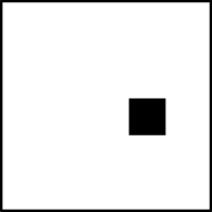
(a) Block pattern

(b) Strip pattern

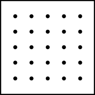
(c) Point pattern

Figure 1: An illustration of three types of failure patterns in 2-dimensional input domains.

Because RT does not make use of any additional information beyond input parameter requirements, research is ongoing into how to improve its testing effectiveness. Adaptive Random Testing (ART) [12] is a family of RT-based testing techniques that aims to improve on RT testing effectiveness by more evenly spreading the test cases throughout the input domain. One of the first, and still most popular, ART implementations is Fixed-Size-Candidate-Set ART (FSCS-ART) [13]. Basically, for each next test case, FSCS-ART randomly generates $k$ candidate test cases, calculates the distance between each candidate and each previously-executed test case (that did not reveal any failure), and selects the candidate furthest from them as the next test case to execute. Many previous studies have demonstrated the high effectiveness of FSCS-ART compared to RT [13, 14, 15, 16, 17, 18]. However, as reported by Wu et al. [19], although ART enhances RT, and is comparable to combinatorial testing in $96\%$ of scenarios, it can be $3.5$ times more computationally expensive than severely-constrained combinatorial testing.

Although ART is very effective, many problems and challenges remain that need to be addressed [12]. One of these problems relates to the time required by FSCS-ART to select test cases, which can be much greater than the execution time: This is referred to as the high computational overhead problem. Many studies have investigated potential performance improvements for ART algorithms, including: a forgetting strategy [20] that reduces the number of distance calculations to previously-executed tests; an approach, DF-FSCS-ART, that ignores executed test cases not in the line of sight of a given candidate [21]; implementations based on a $K$-Dimensional tree (KD-tree) structure, KDFC-ART [22]; a Single-Instruction-Multiple-Data (SIMD) mechanism [23] to calculate all pairwise distances for a single distance calculation instruction; ART-DC [24], which uses a divide-and-conquer strategy to generate the test cases from the entire input domain; and DMART [25], an enhancement of Mirror ART (MART) [26] based on dynamic partitioning, that generates test cases using a specific ART algorithm in half of the sub-domains, and then mirrors these test cases to the other half of the sub-domains to generate the remaining test cases.

As stated, a significant problem faced by FSCS-ART is the heavy time overheads related to the large number of distance calculations required to find the nearest executed test cases for each candidate test case. Alleviating this problem will require a better way of identifying nearest executed test cases. In this paper, we propose a new ART approach using Vantage Point Partitioning (VPP-ART), to improve the efficiency of FSCS-ART. VPP-ART uses a modified VP-tree spatial partitioning structure to avoid redundant distance calculations, reducing the computational overheads of FSCS-ART. An original vantage point tree (VP-tree) [27, 28, 29] is a special kind of spatial partitioning tree that divides the input space into hyperspheres. Using a VP-tree, space can be divided into inner and outer regions of the hypersphere, significantly reducing the number of computations when querying nearest neighbors (NNs) for a given query point. Therefore, vantage point partitioning addresses the need for FSCS-ART time overhead reduction. To evaluate VPP-ART, we conducted a series of simulations and experiments on $22$ subject programs, written in C++ and Java.

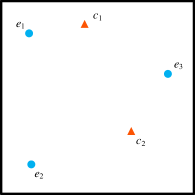
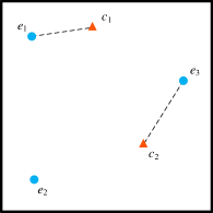
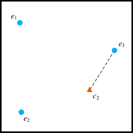
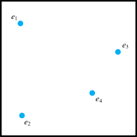
Figure 2: Example illustration of FSCS-ART generating test cases in a 2-dimensional input domain (from Huang et al. [12]).

A standard VP-tree is only applicable to static data — the points must be known before the VP-tree is constructed. However, ART test case generation is a dynamic process: A newly-generated test case $tc$ depends on the information of previously-executed test cases; if no failure is found by $tc$, then $tc$ should be saved in the VP-tree. This process requires that the tree structure support dynamic data, especially insert operations. Because the original VP-tree structure is constructed based on distances between the vantage point and other points, a worst-case scenario exists when a lower-level node in the tree changes, causing upper-level nodes to also (possibly) change, which may necessitate reconstruction of the entire tree. This problem can be addressed by revising the original VP-tree structure to support dynamic data.

The main contributions of this paper are:

• We propose an improved VP-tree structure that can support dynamic insertion. This tree structure can identify an approximate NN that does not differ much from the exact NN, reducing the time cost of FSCS-ART. To the best of our knowledge, this is the first paper to propose using vantage point partitioning to address the ART time overheads problem.

• We report on simulations and experiments investigating VPP-ART, from the perspectives of testing effectiveness and efficiency.

• Compared with FSCS-ART, our approach significantly reduces computational overheads while delivering comparable, or better, failure-detection effectiveness. Compared with KDFC-ART algorithms, our approach has similar or better performance, with reduced time costs in high dimensions.

The rest of this paper is organized as follows: Section 2 introduces some background information about failure patterns, the original FSCS-ART method, and vantage point partitioning. Section 3 presents a framework to enhance FSCS-ART, and introduces VPP-ART. Section 4 describes the simulations and experiments, the results and analyses of which are presented in Section 5. Section 6 discusses the potential threats to the validity of our studies. Related work is discussed in Section 7. Finally, we conclude the paper and discuss some potential future work in Section 8.

2 Background

In this section, we briefly present some background information about failure patterns and Fixed-Size-Candidate-Set ART. We also introduce some preliminary concepts about vantage point partitioning.

2.1 Failure Regions

The inputs to a faulty program can be divided into two distinct types: failure-causing inputs (those inputs which, when executed, cause a test to fail); and non-failure-causing inputs (inputs which do not reveal a failure). The program’s failure region consists of the set of all its failure-causing inputs. In software testing, knowledge of a failure region can be an extremely helpful guide for test case generation and selection. In general, two basic features are used to describe the failure region: the failure pattern, which is the distributions, shape, and locations of failure-causing inputs in the input domain; and the failure rate, denoted $\theta$, which is the proportion of failure-causing to all possible inputs in the entire input domain.

A number of studies [30, 31, 32, 33, 34] have reported that failure-causing inputs tend to cluster into contiguous regions. Chan et al. [35] classified failure patterns into three types: block pattern; strip pattern; and point pattern. Figure 1 shows these three main failure patterns in $2$-dimensional input domains, where the bounding boxes represent the input domain boundaries, and the shaded areas represent the failure regions (containing the failure-causing inputs). Chan et al. [35] also suggested that block and strip patterns are more commonly found than point patterns.

2.2 FSCS-ART: Fixed-Size-Candidate-Set ART

ART is a family of testing methods that improve over RT effectiveness by distributing the test cases more evenly throughout the input domain. One of the first, and still the most popular, ART implementations is Fixed-Size-Candidate-Set ART (FSCS-ART) [13]. Many studies have shown FSCS-ART to be more effective than RT, in terms of failure-detection effectiveness [13, 14, 15, 16], test case distribution [17], and code coverage [18].

FSCS-ART [13] makes use of the concept of distance to evaluate similarities among test cases. It maintains two sets of test cases, the candidate set $C$ and the executed set $E$. $C$ stores $k$ test cases that are randomly generated from the input domain, and $E$ stores the test cases that have already been executed (but without causing any failure). Previous studies [13] have recommended a default value of $10$ for $k$.

The FSCS-ART test case generation process can be described as follows: The first test case, $e_{1}$, is randomly generated from the input domain, and executed. Assuming that $e_{1}$ does not reveal a failure, it is then stored in $E$. From now on, each time a new test case is needed, $k$ test cases are randomly generated, and stored in the candidate set $C$. The best element from $C$ is selected as the next test case to be executed — with FSCS-ART, best is defined as being farthest from the previously-executed test cases (stored in $E$). As testing progresses (without failures being revealed), $E$ grows larger. Formally, given a nonempty set of executed test cases $E$ ($\{e_{1},e_{2},\cdots,e_{|E|}\}$), and a fixed number $k$ of candidate test cases in $C$ ($\{c_{1},c_{2},\cdots,c_{k}\}$), then the requirement for selecting the next (best) test case $c_{\textit{best}}$ is:

$$\min_{\forall e_{i}\in E,c_{j}\in C}dist(c_{j},e_{i})\leq\min_{\forall e_{i}\in E}dist(c_{\textit{best}},e_{i}),$$ (1)

where $dist(x,y)$ is the distance between test cases $x$ and $y$ (typically the Euclidean distance for numerical input domains).

Figure 2 shows an example of FSCS-ART generating test cases in a $2$-dimensional input domain. In the first step of the example (Figure 2), there are three executed test cases, $e_{1}$, $e_{2}$, $e_{3}$ (denoted by small dots); and two candidate test cases, $c_{1}$, $c_{2}$ (denoted by small triangles). In order to select the next test case, the distance between each candidate test case and each executed test case is calculated, and the NN to each candidate is identified. As shown in Figure 2, $e_{1}$ is the NN of $c_{1}$, and $e_{3}$ is the NN of $c_{2}$. The candidate with the greatest distance to its NN — $c_{2}$ in Figure 2 — is selected as the next test case, and executed. If no termination condition is satisfied (e.g., no failure is revealed), then $c_{2}$ is stored in $E$ as the fourth executed test case, $e_{4}$, as shown in Figure 2. This processes continues until a termination condition is satisfied.

A challenge for the FSCS-ART algorithm is its high computational overheads: Each iteration of the FSCS-ART process requires distance calculations between each candidate test case in $C$ and all the previously-executed test cases. The time complexity of FSCS-ART is $O(kN^{2})$, where $k$ is the size of $C$ and $N$ is the number of previously-executed test cases [12]. In order to detect a failure in a program, FSCS-ART could take an enormous amount of time to generate the required number of test cases. When the program’s failure rate is very small, the FSCS-ART time cost will be very high. A key to reducing the computational overheads is to optimize the search for candidates’ nearest executed test cases. Therefore, adoption of the highly-efficient NN Search [36] strategies should enable a reduction in the search time.

2.3 Vantage Point Partitioning

Given a point set in a $d$-dimensional vector space, Vantage Point Partitioning (VPP) [27] makes use of the relative distances between the points and a particular vantage point to enable a very efficient NN search.

VPP can be organized into a tree structure, a Vantage Point tree (VP-tree) [27, 28, 29]. The VP-tree can reduce unnecessary computations when solving NN search problems [36], and has been used in various contexts, including: computational biology [37]; image processing [38]; databases [39, 40]; and computer vision [41]. We have applied some modifications to the original VPP algorithm to enable its use with ART. Our research is, to the best of our knowledge, the first time VP-trees have been applied to test case generation in the field of ART.

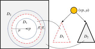
(a) Binary VP-tree

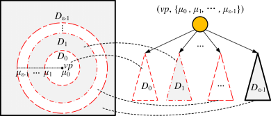
(b) $\varepsilon$-ary VP-tree

Figure 3: VP-tree partitioning strategy in a 2-dimensional input domain.

2.3.1 VP-tree Construction Process

To illustrate the VP-tree construction process, we use an example of binary (2-ary) partitioning. This can easily be generalized to $\varepsilon$-ary cases, where $\varepsilon>2$ [42].

Generally speaking, a binary VP-tree is constructed by splitting a data set into two subsets using a distance partitioning criterion and a vantage point. The vantage point is stored in the root node of the binary VP-tree, and the two subsets are organized into the left and right sub-trees of the root node. Then, the sub-trees are both processed recursively, constructing in each the next level sub-tree according to newly-selected vantage points. This continues until each node contains only one data point, and the construction of the tree is completed. Formally, given a set $\mathcal{D}$ of $n$ data points, a point $vp$ is randomly chosen as the vantage point. Next, the distances between $vp$ and other points in $\mathcal{D}$ are calculated: $\mathcal{S}=\big{\{}dist(p,vp)|p\in\mathcal{D}-\{vp\}\big{\}}$. The entire data set can be partitioned into two subsets using the median distance value $\mu$ in $\mathcal{S}$: As shown in Figure 3(a), $\mathcal{D}_{1}$ refers to the points within a distance of $\mu$ from $vp$; and $\mathcal{D}_{2}$ refers to the points that are more than a distance of $\mu$ from $vp$.

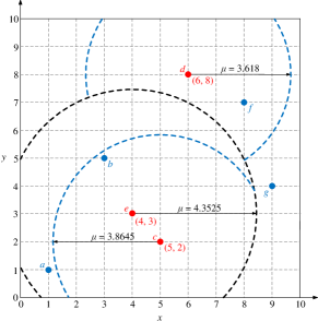
(a) Binary VP-tree partitioning

(b) $\varepsilon$-ary VP-tree partitioning

Figure 4: Example comparison between binary and $\varepsilon$-ary VP-tree partitioning in a 2-dimensional input domain.

The construction process for an $\varepsilon$-ary VP-tree when $\varepsilon>2$, is similar to the binary tree case: For a given set of points ($\mathcal{D}$), a vantage point $vp$ is again randomly chosen, and the distances between $vp$ and all points in $\mathcal{D}$ are calculated and stored in ascending order. The differences compared with the binary case are: (1) the data set is not partitioned into only two subsets, but into $\varepsilon$ approximately-equal subsets, and (2) $vp$ is stored in the first subset (in this paper). As shown in Figure 3(b), $\mu_{i}$ ($i=1,2,\cdots,\varepsilon-1$) denote the boundary distance values that split $\mathcal{D}_{i-1}$ and $\mathcal{D}_{i}$. Formally, for a sequence of distances, stored in ascending order, $\mathcal{S}=\big{\{}dist(a_{j},vp)|a_{j}\in\mathcal{D},j=0,1,\cdots,|\mathcal{D}|-1\big{\}}$, where $|\mathcal{D}|$ is the number of elements in $\mathcal{D}$, the boundary distance values $\mu_{i}$ can be calculated as follows:

$$\mu_{i}=\begin{cases}0,&i=0\\ \frac{\mathcal{S}\Big{(}i\times\big{\lfloor}|\mathcal{D}|/\varepsilon\big{\rfloor}-1\Big{)}+\mathcal{S}\Big{(}i\times\big{\lfloor}|\mathcal{D}|/\varepsilon\big{\rfloor}\Big{)}}{2},&i\in[1,\varepsilon-1]\\ \end{cases}$$ (2)

where $\mathcal{S}(j)$ represents the $j$-th ordered element in $\mathcal{S}$ ($j=0,1,\cdots,|\mathcal{D}|-1$), and $\big{\lfloor}|\mathcal{D}|/\varepsilon\big{\rfloor}$ indicates the rounding down integer $|\mathcal{D}|/\varepsilon$. Therefore, for each point $p$ in $\mathcal{D}_{i}$, the value of $dist(p,vp)$ is between $\mu_{i}$ and $\mu_{i+1}$.

To illustrate the VP-tree construction process, consider a set of data points $\mathcal{D}=\{a,b,c,d,e,f,g\}$ in a 2-dimensional vector space. The binary VPP process is illustrated in Figure 4(a): (1) Point $e$ is randomly selected as the vantage point; (2) the distances between $e$ and all other points are calculated, and stored in $\mathcal{S}$ $=$ $\big{\{}dist(p,e)|p\in\mathcal{D}-\{e\}\big{\}}$ $=$ $\{1.414,2.236,3.606,5.099,5.385,5.657\}$; (3) the median value in $\mathcal{S}$ is calculated — $\mu=(3.606+5.099)/2=4.3525$, in this example; (4) $\mathcal{D}_{1}$ $=$ $\{c,b,a\}$ and $\mathcal{D}_{2}$ $=$ $\{g,d,f\}$ are constructed; (5) the points in $\mathcal{D}_{1}$ and $\mathcal{D}_{2}$ are recursively organized, according to the preceding steps, until each subset contains only one data point. The corresponding binary VP-tree structure is shown in Figure 5(a).

The $\varepsilon$-ary case is illustrated in Figure 4(b), with the final $\varepsilon$-ary VP-tree structure shown in Figure 5(b), where $\varepsilon=3$. Similar to the binary case: (1) Point $e$ is randomly selected as the vantage point; (2) the distances between $e$ and all points are calculated, $\mathcal{S}$ $=$ $\big{\{}dist(p,e)|p\in\mathcal{D}\big{\}}$ $=$ $\{0.000,1.414,2.236,3.606,5.099,5.385,5.657\}$; (3) three boundary values are defined —

$$\mu_{0} =0.000,$$

$$\mu_{1} =\frac{\mathcal{S}\Big{(}\big{\lfloor}7/3\big{\rfloor}\times 1-1\Big{)}+\mathcal{S}\Big{(}\big{\lfloor}7/3\big{\rfloor}\times 1\Big{)}}{2}$$

$$=\frac{\mathcal{S}(1)+\mathcal{S}(2)}{2}=\frac{1.414+2.236}{2}=1.825,$$

$$\mu_{2} =\frac{\mathcal{S}\Big{(}\big{\lfloor}7/3\big{\rfloor}\times 2-1\Big{)}+\mathcal{S}\Big{(}\big{\lfloor}7/3\big{\rfloor}\times 2\Big{)}}{2}$$

$$=\frac{\mathcal{S}(3)+\mathcal{S}(4)}{2}=\frac{3.606+5.099}{2}=4.353,$$

partitioning $\mathcal{D}$ into three approximately-equally-sized subsets; (4) the steps above are repeated in each subset.

2.3.2 Nearest Neighbor Search in a VP-tree

This section describes the algorithm for an NN search in a VP-tree, which involves identifying the nearest neighboring point of a query point $q$ with the requirement that the maximum distance between $q$ and the point be less than a specific threshold $\sigma$. This means that if the distance between $q$ and its neighbor is greater than $\sigma$, then this cannot be the NN. If $dist(q,vp)$ is the distance between the query point $q$ and the vantage point $vp$, then the algorithm focuses on finding the NN of $q$ within the range $dist(q,vp)\pm\sigma$. With these requirements, the search for the NN of $q$ in a binary VP-tree only needs to explore both $\mathcal{D}_{1}$ and $\mathcal{D}_{2}$ if $q$ is in the range of $[\mu-\sigma,\mu+\sigma]$ (as shown in Figure 3(a)) — otherwise, only one subset needs to be searched, which effectively prunes one half of the input space. The approach is based on the principles of triangular inequality. Formally, if $dist(q,vp)\leq\mu-\sigma$, for $p\in\mathcal{D}_{2}$, the distance between $p$ and $q$ is lower-bounded by $\sigma$ [29]:

$$dist(p,q)\geq ~{}\Big{|}\big{|}dist(p,vp)\big{|}-\big{|}dist(q,vp)\big{|}\Big{|}$$ (3)

$$\geq ~{}\Big{|}\big{|}dist(p,vp)\big{|}-(\mu-\sigma)\Big{|}$$

$$> ~{}|\mu-\mu+\sigma|$$

$$= ~{}\sigma,$$

therefore, the subset $\mathcal{D}_{2}$ can be ignored. Similarly, if $dist(q,vp)>\mu+\sigma$, for $p\in\mathcal{D}_{1}$, then $\mathcal{D}_{1}$ can be ignored. For the $\varepsilon$-ary cases, the system needs to explore $\mathcal{D}_{i}$ if:

$$\mu_{i}-\sigma<d(q,vp)\leq\mu_{i+1}+\sigma,$$ (4)

for $i=0,1,\cdots,\varepsilon-2$ (the special case of $i=\varepsilon-1$ will be discussed in Section 3.2.3): It is also based on triangular inequality, and can be derived in a similar way to the binary case.

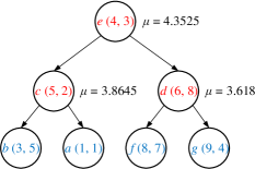
(a) Binary VP-tree structure

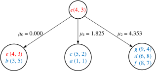
(b) $\varepsilon$-ary VP-tree structure

Figure 5: Example of the comparison between binary VP-tree structure and $\varepsilon$-ary VP-tree structure in a 2-dimensional input domain.

3 VPP-ART: ART based on Vantage Point Partitioning

In this section, we present our proposed ART approach, Vantage Point Partitioning ART (VPP-ART).

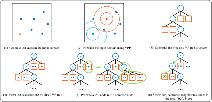
Figure 6: The VPP-ART framework, with six main stages.

3.1 Framework

A main challenge for FSCS-ART lies in the high time cost in generating test cases. In this paper, we combine vantage point partitioning with the original FSCS-ART to improve the efficiency, mainly by organizing the set of executed test cases into a new storage structure. As noted, ART requires that the data structure used to store the executed test cases be able support dynamic insertion.

The entire VPP-ART approach is similar to that of FSCS-ART. (1) Initially, a test case is randomly generated within the input domain. This test case is used to execute the SUT, and, if no testing termination condition is met, then this test case is added to the modified VP-tree. (2) Thereafter, $k$ candidate test cases are randomly generated in each round, and (temporarily) stored in the candidate test case set $C$. (3) The best candidate in $C$ is determined using a search strategy to find all candidates’ NNs in the modified VP-tree, with the candidate whose minimum distance is greatest then selected (Equation 1).

In general, typical testing termination conditions include: (1) at least one failure has been detected in the program under test; and (2) the number of executed test cases has reached some predetermined threshold value. When the termination condition is satisfied, the entire testing process ends.

The framework is shown in Figure 6. In the figure, the small squares represent the vantage points, the dots represent executed test cases, and the star represents a newly-generated test case. The framework consists of six main stages: (1) Generate test cases in the input domain; (2) Partition the input domain using VPP; (3) Construct the modified VP-tree structure; (4) Insert test cases into the modified VP-tree; (5) Promote a leaf node into a common node; and (6) Search for the NN test cases in the modified VP-tree.

Stage 1: The test cases are generated in the same way as in FSCS-ART. The candidate test case set ($C$) contains $k$ test cases randomly generated in the input domain. The executed test cases are stored in a modified VP-tree. Similar to FSCS-ART, the Euclidean distance is used to measure the similarity (distance) between test cases.

Stage 2: As the testing process proceeds, VPP is used to partition the input domain into different concentric hypersphere sub-domains, bounded by different vantage points. Each sub-domain contains far fewer test cases than the number of executed test cases in the entire input domain.

Stage 3: A modified VP-tree structure that supports dynamic data is used to store executed test cases, and to support the NNs searches.

Stage 4: As VPP-ART proceeds, the candidate test cases ($C$) are generated randomly within the input domain, and the best candidate is identified and applied to the SUT. If an SUT failure is not revealed (and no other testing termination criteria are met), then the test case is added to the modified VP-tree. As the testing continues, the number of executed test cases in the VP-tree increases.

Stage 5: Test cases are only stored in leaf nodes of the modified VP-tree. During test case insertion, the number of test cases in a leaf node may reach the storage capacity, causing a promotion operation to be performed, which expands the storage capacity of the leaf node. Each round of test case insertion only needs to be executed, at most, once. After at most one promotion operation, a suitable leaf node (with spare capacity) will be identified and used to store the current test case.

Stage 6: The executed NN for each candidate test case is identified using the $\varepsilon$-ary VP-tree, with a series of query thresholds $\sigma$ used to perform the searches. Starting from the root node of the modified VP-tree, the distances to vantage test cases are compared, layer by layer, until the leaf node containing the NN is identified.

3.2 Algorithm

The original VP-tree structure is constructed according to the distance criterion. The $top$-$down$ partitioning strategy makes the management of VP-tree updates complicated — the partitioning of upper-level nodes has an impact on the partitioning of lower-level nodes [42]. In a worst-case scenario, reconstruction of the entire tree structure may be required. The VP-tree update operation remains a problem requiring further study. Fu et al. [42] proposed a dynamic VP-tree structure, but this strategy involving upward backtracking and node-splitting/merging, which may incur significant time overheads.

In this paper, we (1) introduce a modified VP-tree structure in which to store the executed FSCS-ART test cases; and (2) propose an insertion approach for this modified structure, the pseudo-code for which is in Algorithm 1.

Inputs: 

The candidate set size, $k$;

The number of dimensions in the SUT input domain, $d$;

The capacity of a leaf node, $\lambda$;

The partitioning parameter, $\varepsilon$;

Output: 

The VP-tree with executed test cases, $T$;

1:  Set $T\leftarrow\{\}$; /* Initially, VP-tree for storing the executed test

cases is empty. */

2:  Set $C\leftarrow\{\}$; /* Initially, candidate test case set $C$, for storing $k$

candidates in each round, is empty. */

3:  Set $min_{\textit{dist}}[k]\leftarrow\infty$; /* Initially, the minimum distance between

each candidate test case and $T$ is set to infinity. */

4:  Randomly generate a test case $tc$ from the input domain

5:  Execute $tc$;

6:  while (No termination condition is satisfied) 

7:     InsertTCIntoVPtree($tc$, $\lambda$, $\varepsilon$, $node$);

8:     Randomly generate $k$ candidate test cases $c_{1},c_{2},\cdots,c_{k}$

from the input domain, then set $C\leftarrow\{c_{1},c_{2},\cdots,c_{k}\}$;

9:     for (each candidate $c_{j}\in C$, where $j=1,2,\cdots,k$) 

10:        Set $min_{\textit{dist}}[j]\leftarrow$ GetMinDistFromVPtree($c_{j}$, $node$);

11:     end_for

12:     Find $c_{\textit{best}}$ from $c_{1},c_{2},\cdots,c_{k}$ having the maximum

distance from its nearest test case;

13:     Set $tc\leftarrow c_{\textit{best}}$ and execute $tc$;

14:  end_while

15:  return  $T$;

Algorithm 1 VPP-ART

3.2.1 Modified VPP-ART VP-tree structure

Figure 7 shows the modified VP-tree structure, where nodes are divided into leaf nodes and common nodes, denoted by circles and squares, respectively. Leaf nodes contain only test cases, the maximum number of which that can be stored in a single leaf node is denoted by $\lambda$. Common nodes contain no test cases, but do contain the vantage test case information, several boundary distance values with child pointers, and an NN threshold.

The partitioning parameter, $\varepsilon$, specifies the number of subsets per division. This determines the number of child pointers in each common node ($c_{0},c_{1},\cdots,c_{\varepsilon-1}$ in Figure 7). The child pointers point to nodes in the next level of the tree. The same $\varepsilon$ value is used for each partition, with this value being set by the tester.

Vantage test cases are at the core of the structure, and their choice, in each level of the VP-tree, plays an important role in the performance of the algorithm. An ideal vantage test case should have a uniform distribution of distances between it and other test cases. This minimizes the number of test cases in concentric regions, thereby reducing the probability that all sub-trees must be explored. However, finding the ideal vantage test case for a given test case set can require very heavy computational costs. In practice, therefore, a test case is randomly selected from the $\lambda$ test cases stored in a leaf node, yielding an approximate (instead of optimal) vantage test case. This selection method has been shown to be effective, experimentally.

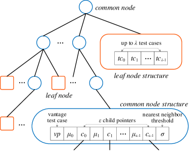
Figure 7: The modified VPP-ART VP-tree structure.

3.2.2 VPP-ART Test Case Insertion Algorithm

The VP-tree update operations, especially insertion, have a crucial role in the effectiveness of VPP-ART. In the following, we focus on the VPP-ART test case storage process, and propose insert and node promotion strategies to make this process more dynamic.

Inputs: 

The executed test case need to insert into the tree, $tc$;

The capacity of a leaf node, $\lambda$;

The number of subsets partition, $\varepsilon$;

A node of the VP-tree, $node$;

Output: 

Success flag, FALSE or TRUE;

1:  if ($node$ is $tc$-QBN (a leaf node)) 

2:     if ($|tc$-QBN$|<\lambda$) 

3:        Insert tc into $tc$-QBN;

4:        Set $tc$-BN $\leftarrow$ $tc$-QBN;

5:        return  TRUE;

6:     else if ($|tc$-QBN$|=\lambda$) /* Node promotion strategy */ 

7:        Randomly select a test case from $tc$-QBN, as the vantage

test case, $vp$;

8:        for (each test case $p\in tc$-QBN $\cup\{tc\}$) 

9:           Calculate $dist(p,vp)$;

10:           Sort the test cases in ascending order according to the

distance values;

11:        end_for

12:        Calculate the boundary distance values $\mu_{i}$ according to

Equation 2;

13:        Calculate $\sigma$ of current node, using Equation 6;

14:        Partition the input domain into $\varepsilon$ sub-domains;

/* Each sub-domain contains approximately the same

number of test cases */

15:        Reorganize all the test cases to the children nodes of this

new common node;

16:        if (allocate the new $tc$-BN) 

17:           return  TRUE;

18:        end_if

19:     end_if

20:  else

21:     Calculate $dist(vp,tc)$;

22:     if ($\mu_{i}<dist(vp,tc)\leq\mu_{i+1}$ where $0\leq i\leq\varepsilon-2$) 

23:        InsertTCIntoVPtree($tc$, $\lambda$, $\varepsilon$, $node.i$-th child node);

24:     end_if

25:     if ($dist(vp,tc)>\mu_{\varepsilon-1}$) 

26:        InsertTCIntoVPtree($tc$, $node.(\varepsilon-1)$-th child node);

27:     end_if

28:  end_if

Algorithm 2 InsertTCIntoVPtree($tc$, $\lambda$, $\varepsilon$, $node$)

Insertion: As testing progresses, it becomes necessary to insert newly-generated test cases into the modified VP-tree. For an executed test case $e$, if the current node is a leaf node, then the leaf node is said to be the quasi-belonging-node for $e$ (denoted $e$-QBN). If the number of test cases in $e$-QBN is less than the maximum storage capacity ($\alpha<\lambda$), then $e$ is inserted into $e$-QBN, and $e$-QBN is said to be the belonging-node for $e$ (denoted $e$-BN). If $\alpha=\lambda$, then it is necessary to promote (reconstruct) $e$-QBN to find $e$-BN. If the current node is a common node, then $dist(e,vp)$ is calculated (where $vp$ is the vantage test case in this node), and compared with the boundary values $\mu_{i}$ to determine which child pointer should be followed to find $e$-BN.

Promotion: This step is only performed when $\alpha=\lambda$, which means that it is necessary to transform $e$-QBN from a leaf node into a common node. A test case $t_{i}$ $(0<i\leq\lambda)$ is randomly selected from the test cases stored in $e$-QBN as the vantage test case for this node; the remaining test cases and $e$ are reorganized into child nodes (new leaf nodes) of this new common node; and $e$ is assigned to its new $e$-BN. This promotion process is executed, at most, one time when inserting $e$: After (at most) one promotion process, VPP-ART will find an $e$-BN in which to store $e$. The Insertion/Promotion pseudo-code is listed in Algorithm 2.

3.2.3 Approximate Nearest Neighbor Search in VPP-ART

In this section, the approach to calculate $\sigma$ is discussed, and the VPP-ART approximate NN search process is explained.

Nearest neighbor threshold: As discussed in Section 2.3.2, the threshold value $\sigma$ is the key to the search algorithm. It can be used to reduce the NN search effort such that the NNs of a query point are always very close to the query point itself — in other words, the smallest possible value of $\sigma$ can be used. Chiueh et al. [29] proposed a minimum possible value of $\sigma$, which we adopted and modified to match our partitioning strategy. Upper ($u[i]$) and lower ($l[i]$) bounds exist for distances in the $i$-th subset $\mathcal{D}_{i}$ of the partitioned input domain: $u[i]$ is the distance from the farthest test case in the current subset to its corresponding vantage test case, and $l[i]$ is the distance from the nearest test case. When traversing the VP-tree, it is not necessary to explore the nearest executed test cases of a candidate $c$ in $\mathcal{D}_{i}$ if $dist(c,vp)>u[i]+\sigma$, or $dist(c,vp)<l[i]-\sigma$. This use of $\sigma$ guarantees that $dist(c,vp)$ will fall within at least one of the ranges in $\big{[}l[i]-\sigma,u[i]+\sigma\big{]}$: This means that the search operation can be performed (and completed) in one sub-domain of the entire input domain. For each common node, the upper and lower bounds of $\varepsilon$ partitioned subsets are computed as:

$$\sigma_{i}=\frac{l[i]-u[i-1]}{2},$$ (5)

and the default value of $\sigma$ (for that node) is chosen to be the maximum value from $(\varepsilon-1)$ values, as determined by:

$$\sigma=\max_{i=1}^{\varepsilon-1}\sigma_{i}.$$ (6)

Based on the relationship among $\sigma$, $\mu$, and $dist(c,vp)$, VPP-ART can start from the root node of the modified VP-tree and recursively search downwards until it finds the leaf node that contains the nearest executed test case of the current candidate.

Combined with the partitioning boundary values in Figure 3(b), the last sub-domain ($\mathcal{D}_{\varepsilon-1}$) defined in Equation 4 is not covered by the search process. The reason for this is that the possible values of $i$ can only be from $0$ to $\varepsilon-2$. When $dist(q,vp)>\mu_{\varepsilon-1}$, the NN search process cannot be executed in $\mathcal{D}_{\varepsilon-1}$. To solve this, $\mathcal{D}_{\varepsilon-1}$ is treated separately: If $dist(q,vp)>\mu_{\varepsilon-1}$, then an exhaustive search in $\mathcal{D}_{\varepsilon-1}$ is conducted to obtain the query point $q$, and to get the NN distance in $\mathcal{D}_{\varepsilon-1}$. This will mean that the NN of $q$ — which located at the boundary of $\mathcal{D}_{\varepsilon-2}$ and $\mathcal{D}_{\varepsilon-1}$ — may be in the $\mathcal{D}_{\varepsilon-2}$, while the VPP-ART only searches in the $\mathcal{D}_{\varepsilon-1}$, and finds an approximate NN, rather than an exact NN.

Inputs: 

A candidate test case, $c_{j}$;

A node of the VP-tree, $node$;

Output: 

The minimum distance between $c_{j}$ and $E$, $min_{\textit{dist}}[j]$;

1:  $min_{\textit{dist}}[j]\leftarrow\infty$;

2:  if ($node$ is leaf node) 

3:     for (each test case $p$ in $node$) 

4:        if ($dist(c_{j},p)<min_{\textit{dist}}[j]$) 

5:           $min_{\textit{dist}}[j]\leftarrow dist(c_{j},p)$;

6:        end_if

7:     end_for

8:     return  $min_{\textit{dist}}[j]$;

9:  else

10:     Calculate $dist(c_{j},vp)$;

11:     for ($0\leq i\leq\varepsilon-2)$) 

12:        if ($\mu_{i}-\sigma<dist(vp,c_{j})\leq\mu_{i+1}+\sigma$) 

13:           Get $\sigma$ of current common node;

14:           GetMinDistFromVPtree($c_{j}$, $node.i$-th child node);

15:        end_if

16:     end_for

17:     if ($dist(c_{j},vp)>\mu_{\varepsilon-1}$) 

18:        GetMinDistFromVPtree($c_{j}$, $node.(\varepsilon-1)$-th child node);

19:     end_if

20:  end_if

Algorithm 3 GetMinDistFromVPtree($c_{j}$, $node$)

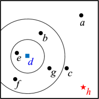
(a) Insertion

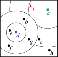
(b) Promotion

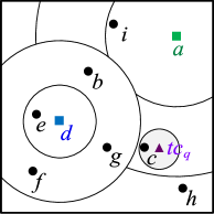
(c) Search

Figure 8: Illustration of VPP-ART insertion, promotion, and search strategies in a 2-dimensional input domain.

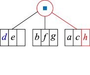
(a) Insert into a leaf node

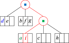
(b) Promote a leaf node

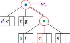
(c) Search for the NN in the tree

Figure 9: Illustration of insertion, promotion, and searching strategies in the modified VP-tree (in a 2-dimensional input domain). These modified VP-tree structures correspond to Figure 8.

Approximate Nearest Neighbor Search: The NN obtained by VPP-ART could be an approximate NN, because this search process is likely to find an inaccurate neighbor in the leaf node that does not contain an exact NN, which can be explained as follows: (1) Some specific sub-domains need special consideration, and the entire search may be carried out in these sub-domains, which may not contain the exact NNs. Such as the last sub-domains ($\mathcal{D}_{\varepsilon-1}$) after each round of partitioning. (2) Because the boundary distance $\mu$ and the NN threshold $\sigma$ of each node are calculated according to the fixed number of test cases, these two values of each node will be affected when a new point is inserted. To a certain extent, VPP-ART deliberately ignores the impact of the insertion process on these two values. Specifically, when a new point is inserted, VPP-ART ignores the change of the two values of the QBN’s upper-level nodes — it does not update their $\mu$ and $\sigma$ values. This may cause the NN of the query point to no longer be in the original sub-domain, which reduces the accuracy of the search algorithm.

Although VPP-ART adopts an approximate NN search, it still has advantages in some cases: (1) For an exact NN, an exhaustive search will be executed — the distances between the executed test cases and the candidate will all be calculated, and the closest executed test case will be identified as the NN. When the number of test cases is very large, or the dimensionality is relatively high, the search efficiency decreases sharply. However, VPP-ART can obtain a better efficiency by using an approximate search: VPP-ART can identify an acceptable NN using fewer distance calculations when searching for an approximate NN. (2) An approximate NN search process, by not being limited to identifying the exact NN, can improve the search efficiency at an acceptable cost in the accuracy. When searching some sub-domains, the accuracy of some NNs may be lost, but VPP-ART may achieve similar, or even better, results than other exact NN-based ART algorithms. The difference between approximate NN and exact NN can be very small, enabling VPP-ART to have comparable failure-detection effectiveness. (3) Using the characteristic that test cases closer to the vantage point are more likely to be divided into the same sub-domain. When the number of test cases increases, test cases with greater similarity will aggregate together. Using the VP-tree structure, VPP-ART, according to the distance relationship between candidate test cases and vantages points, will search the possible sub-domains (leaf nodes in the VP-tree) of executed test cases with greater similarity to candidate test cases.

The pseudo-code for the search process is listed in Algorithm 3.

3.2.4 Examples of VPP-ART operations

Figure 8 shows examples of insertion, promotion, and searching with VPP-ART, in a $2$-dimensional input domain. The corresponding VP-tree structures are shown in Figure 9, where $\lambda=3$, $\varepsilon=3$.

Insertion: Test case $h$ is a newly-generated test case for which no software failure is found and needs to be inserted into the VP-tree (Figure 8(a)). At this point, the third leaf node of the tree defined by the vantage test case $d$ still has space for the test case, so it is inserted directly (Figure 9(a)).

Promotion: Test case $i$ is the newly-generated test case that has revealed no software failure. It needs to be inserted into the VP-tree (Figure 8(b)). The third leaf node of the VP-tree defined by the vantage test case $d$ has no space to accommodate $i$, so the promotion operation is executed. During promotion, $a$ is randomly selected as the vantage test case from $a$, $c$, and $h$). The third sub-domain defined by the vantage test case $d$ is redistributed, and the four test cases are reorganized to three leaf nodes according to the distance values in $\mathcal{S}=\big{\{}dist(i,a),dist(c,a),dist(h,a)\big{\}}$. Finally, test case $i$ is then inserted into the first node of $a$ (Figure 9(b)).

Search: For queries with nearest executed test cases, a candidate test case $tc_{q}$ needs to find the NN in the input domain (Figure 8(c)). Starting from the root of the tree, the leaf nodes containing the NNs are searched, layer by layer, based on the partitioning radius $\mu$, the query threshold $\sigma$, and the distance relations defined in Section 2.3.2. In this example, if the second leaf node defined by the vantage point $a$ contains the NN, and this leaf node contains only $c$, then $c$ is considered the NN for $tc_{q}$ (Figure 9(c)).

4 Experimental Studies

This section introduces the design and settings of the simulations and experiments that we conducted to evaluate VPP-ART.

4.1 Research Questions

The proposed VPP-ART algorithm aims to reduce the time overheads of the original FSCS-ART algorithm, thus, measurement and examination of the test case generation time is necessary. VPP-ART is also expected to maintain the FSCS-ART failure-detection effectiveness, which requires evaluation and verification in various scenarios. The experimental studies were guided by the following research questions:

• How well does VPP-ART perform, in terms of software failure-detection, compared with other ART algorithms?

• Compared with FSCS-ART and KDFC-ART, to what extent can VPP-ART reduce computational overheads?

4.2 Variables and Evaluation Metrics

This section describes the independent and dependent variables in our research. The evaluation metrics used to examine the effectiveness and efficiency of the different ART algorithms are also introduced.

4.2.1 Independent Variable

The independent variable in the experimental study are the different ART algorithms used to generate test cases. VPP-ART, the new algorithm proposed in this paper, is compared with FSCS-ART [13] and KDFC-ART [22].

VPP-ART is an enhanced version of FSCS-ART, and we want to know the effects of using VPP on FSCS-ART. The KD-tree is an efficient spatial indexing mechanism. Mao et al. [22] introduced KD-trees into ART, and proposed three KDFC-ART algorithms: Naive-KDFC; SemiBal-KDFC; and LimBal-KDFC. Naive-KDFC and SemiBal-KDFC search for the exact NN of candidate test cases, and thus their generated test cases are the same as those generated by FSCS-ART. LimBal-KDFC uses a limited backtracking method, identifying an approximate NN, similar to VPP-ART. The simulations and experiments sought to examine two things: (1) the impact of the difference between exact and approximate NN searching on ART effectiveness and efficiency; and (2) the differences in effectiveness and efficiency between the two approximate NN-search-based ART algorithms, VPP-ART and LimBal-KDFC.

4.2.2 Dependent Variables

The dependent variables in our studies are the evaluation metrics, for both effectiveness and efficiency.

Effectiveness Metrics The F-measure [14] gives the number of test case executions before detecting the first failure in the SUT, and has been widely used in ART studies [12]. We also used the F-measure as an evaluation metric in our study, with $F_{\textit{RT}}$ and $F_{\textit{ART}}$ denoting the F-measure when conducting RT and ART, respectively. Theoretically, $F_{\textit{RT}}$ equals to $1/\theta$ (where $\theta$ is the SUT failure rate). The ART F-ratio [14] denotes the ratio of $F_{\textit{ART}}$ to $F_{\textit{RT}}$, showing the improvement of ART over RT: A lower ART F-ratio indicates better ART performance.

Efficiency Metrics There are several measurements commonly taken when examining the efficiency of a testing methodology, including: generation time; execution time; and F-time [12] [43]. The generation time refers to the cost of generating k test cases; the execution time refers to the time cost of executing the SUT with k test cases; and the F-time [43] is defined as the entire time cost for finding the first failure in the SUT. Generally speaking, the test case generation time has a great impact on the entire test cost. For the simulation studies, we recorded the average generation time to generate a certain number of test cases.

4.3 Experimental Environment

The simulations and experiments were conducted using a 16-GB RAM laptop PC with an i7 CPU, running at 2.20 GHz, running under the 64-bit Windows 10 operating system. All the algorithms under study were implemented in Java with JDK 1.8. The IDEs used were Eclipse (Version 4.15.0) and Microsoft Visual Studio 2019.

4.4 Data Collection and Statistical Analysis

The F-measure and F-time values were calculated by running each of the ART algorithms until a failure was detected. In the simulations, a failure was considered to be detected whenever a test case was generated from within a simulated failure region. In the experiments, the actual output was compared with the expected output (the test oracle [3], [4], [5]): A difference indicated a failure being detected. To minimize the error caused by randomness, and to provide confidence in the comparison, each experiment was run 3000 times, with the average being recorded.

When analyzing the experimental data, the p-value (probability value) and effect size for the different ART algorithms were calculated [44], [45], [46]. These can describe any significant differences or improvements between the two compared methods [47]. The unpaired two-tailed Mann-Whitney-Wilcoxon test [46] was used to verify whether or not there was a significant differences among the investigated ART algorithms. A p-value less than $0.05$ indicates a significant difference between the two algorithms [48]. The effect size [46] shows the possibility that one method is better than another: We used the non-parametric Vargha and Delaney effect size [49]. For two methods, A and B, an effect size between A and B of $0.50$ means that A and B are equivalent; if the value is greater than $0.50$, A is better than method B; and if the value is less than $0.50$, B is better than method A.

TABLE I: 22 subject programs used in experiments

No.	Program	Dimension $(d)$	Input domain		Size (LOC)	Mutant Operators	Total Faults
			From	To
1	airy	1	-5000	5000	43	CR	1
2	bessj0	1	-300000	300000	28	AOR, ROR, SVR, CR	5
3	erfcc	1	-30000	30000	14	AOR, ROR, SVR, CR	4
4	probks	1	-50000	50000	22	AOR, ROR, SVR, CR	4
5	tanh	1	-500	500	18	AOR, ROR, SVR, CR	4
6	bessj	2	(2, -1000)	(300, 15000)	99	AOR, ROR, CR	4
7	gammq	2	(0, 0)	(1700, 40)	106	ROR, CR	4
8	sncndn	2	(-5000, -5000)	(5000, 5000)	64	ROR, CR	5
9	golden	3	(-100, -100, -100)	(60, 60, 60)	80	ROR, SVR, CR	5
10	plgndr	3	(10, 0, 0)	(500, 11, 1)	36	AOR, ROR, CR	5
11	cel	4	(0.001, 0.001, 0.001, 0.001)	(1, 300, 10000, 1000)	49	AOR, ROR, CR	3
12	el2	4	(0, 0, 0, 0)	(250, 250, 250, 250)	78	AOR, ROR, SVR, CR	9
13	calDay	5	(1, 1, 1, 1, 1800)	(12, 31, 12, 31, 2200)	37	SDL	1
14	complex	6	(-20, -20, -20, -20, -20, -20)	(20, 20, 20, 20, 20, 20)	68	SVR	1
15	pntLinePos	6	(-25, -25, -25, -25, -25, -25)	(25, 25, 25, 25, 25, 25)	23	CR	1
16	triangle	6	(-25, -25, -25, -25, -25, -25)	(25, 25, 25, 25, 25, 25)	21	CR	1
17	line	8	(-10, -10, -10, -10, -10, -10, -10, -10)	(10, 10, 10, 10, 10, 10, 10, 10)	86	ROR	1
18	pntTrianglePos	8	(-10, -10, -10, -10, -10, -10, -10, -10)	(10, 10, 10, 10, 10, 10, 10, 10)	68	CR	1
19	twoLinesPos	8	(-15, -15, -15, -15, -15, -15, -15, -15)	(15, 15, 15, 15, 15, 15, 15, 15)	28	CR	1
20	nearestDistance	10	(1, 1, 1, 1, 1, 1, 1, 1, 1, 1)	(15, 15, 15, 15, 15, 15, 15, 15, 15, 15)	26	CR	1
21	calGCD	10	(1, 1, 1, 1, 1, 1, 1, 1, 1, 1)	(1000, 1000, 1000, 1000, 1000, 1000, 1000, 1000, 1000, 1000)	24	AOR	1
22	select	11	(1, 1, 1, 1, 1, 1, 1, 1, 1, 1, 1)	(10, 100, 100, 100, 100, 100, 100, 100, 100, 100, 100)	117	RSR, CR	2

4.5 Simulations and Experiments

The original FSCS-ART and KDFC-ART algorithms were compared with our proposed algorithm, VPP-ART, through a series of simulations and experiments [12]. The simulations involved simulated software faults, while the experiments used real-life subject programs altered through mutation analysis techniques [50].

4.5.1 Simulations Design

The simulations used a $d$-dimensional hypercube as the program input domain ($\mathcal{D}$). $\mathcal{D}$ was set as $\big{\{}(x_{1},x_{2},\cdots,x_{d})|0.0$ $\leq$ $x_{1},x_{2},\cdots,x_{d}<$ $1.0\big{\}}$, with the dimensionality, $d$, set as $1$, $2$, $3$, $4$, $5$, $8$ and $10$.

To address RQ1, the simulated failure regions were randomly placed in the input domain $\mathcal{D}$. Once a program has been written, the failure regions are fixed, but their locations are unknown to developers and testers (before testing). Failure regions have geometric shape (described by the failure patterns) and size (described by the failure rate), and distribution [12]. In the simulations, the failure rate and pattern were set in advance, allowing the failure regions to be located randomly in $\mathcal{D}$. As described in Section 2.1, failure patterns have often been categorized into three main types: strip; block; and point. The simulations included all three failure patterns types. Block patterns used a randomly-located, single-solid shape with equal lengths of side — a square in $2$-dimensions, cube in $3$-dimensions, etc. The strip patterns were each constructed using two points on adjacent boundaries that were connected with a width/volume to yield the desired size. According to the predetermined failure rate $\theta$, the point patterns used $25$ randomly-located regions. The simulations used seven different $\theta$ settings: $0.01$, $0.005$, $0.002$, $0.001$, $0.0005$, $0.0002$ and $0.0001$.

To address RQ2, the simulations recorded the test case generation times for both FSCS-ART and VPP-ART. A total of $20$,$000$ test cases were generated by each algorithm in the $d$-dimensional input domain, and the generation times recorded at intervals of $500$.

4.5.2 Experiments Design

Although simulations can simulate the performance of the algorithms in different scenarios, the failure types may not be representative of real-life situations for example, in reality, the failure types can be categorized into regular and irregular types [51] [52]). In addition to the simulations, we conducted experiments using 22 real-life programs with faults seeded in using mutation operators [50]. Table I presents the detailed information of these programs. 12 of the programs come from Numerical Recipes [53] and ACM’s Collected Algorithms [54], and have been widely studied in ART research [13, 16, 55, 25]. Programs calDay, complex, and line are from Ferrer et al. [56]. The pntLinePos, pntTrianglePos and twoLinesPos programs describe the positional relationships between a point and a line, a point and a triangle, and between two lines, respectively [57]. The triangle program classifies a triangle into one of three types (acute, right and obtuse) [57]. The nearestDistance program uses five points to realize the nearest point pair function. The calGCD program calculates the greatest common divisor of $10$ integers, and select returns the $i$-th largest element from an unordered array [58].

All subject programs were implemented in Java or C++, and had previously been used in the KDFC-ART experiments [22]. Six mutation operators were used to generate mutants of the original subject programs [50]: (1) arithmetic operator replacement (AOR); (2) relational operator replacement (ROR); (3) scalar variable replacement (SVR); (4) constant replacement (CR); (5) statement deletion (SDL); and (6) return statement replacement (RSR). Five algorithms were applied in the experiments: the original FSCS-ART; the three KDFC-ART algorithms; and our proposed VPP-ART.

TABLE II: ART F-ratio values of VPP-ART with different $\langle\varepsilon,\lambda\rangle$ parameter pair values

Partitioning Number $(\varepsilon)$	Dimension $(d)$	ART F-ratio
		FSCS-ART	VPP-ART
			$\lambda=10$	$\lambda=15$	$\lambda=20$	$\lambda=25$	$\lambda=30$	$\lambda=35$	$\lambda=40$	$\lambda=45$	$\lambda=50$
$\varepsilon=2$	$d=1$	0.5564	0.5706	0.5652	0.5523	0.5611	0.5675	0.5747	0.5631	0.5634	0.5702
	$d=2$	0.6391	0.6790	0.6584	0.6752	0.6712	0.6645	0.6547	0.6641	0.6516	0.6440
	$d=3$	0.7549	0.8056	0.7890	0.7809	0.7787	0.7964	0.8053	0.7957	0.8096	0.7970
	$d=4$	0.9033	0.9611	0.9329	0.9243	0.9391	0.9506	0.9539	0.9280	0.9368	0.9462
	$d=5$	1.0462	1.0824	1.0945	1.0984	1.0852	1.0978	1.1147	1.1260	1.1200	1.1069
	$d=8$	1.8607	1.7050	1.6886	1.7668	1.7673	1.8200	1.7956	1.7711	1.8460	1.8289
	$d=10$	2.6138	2.4504	2.4896	2.6366	2.6495	2.6355	2.6268	2.7046	2.7357	2.7719
$\varepsilon=3$	$d=1$	0.5564	0.5555	0.5605	0.5686	0.5584	0.5557	0.5573	0.5599	0.5514	0.5582
	$d=2$	0.6391	0.6510	0.6601	0.6447	0.6559	0.6377	0.6661	0.6459	0.6725	0.6523
	$d=3$	0.7549	0.7553	0.7534	0.8083	0.7832	0.7753	0.7663	0.8063	0.8037	0.7940
	$d=4$	0.9033	0.9390	0.9448	0.9510	0.9385	0.9385	0.9345	0.9355	0.9484	0.9421
	$d=5$	1.0462	1.0605	1.0890	1.0709	1.0698	1.1085	1.0876	1.0997	1.1178	1.1053
	$d=8$	1.8607	1.6631	1.8007	1.7354	1.7543	1.8558	1.8406	1.8833	1.8870	1.8493
	$d=10$	2.6138	2.2916	2.4821	2.4765	2.5670	2.6265	2.6319	2.7906	2.7058	2.7080
$\varepsilon=4$	$d=1$	0.5564	0.5577	0.5636	0.5621	0.5613	0.5529	0.5726	0.5567	0.5607	0.5588
	$d=2$	0.6391	0.6570	0.6587	0.6590	0.6739	0.6534	0.6296	0.6340	0.6448	0.6529
	$d=3$	0.7549	0.7617	0.7680	0.7571	0.7604	0.7659	0.7519	0.7900	0.7709	0.7754
	$d=4$	0.9033	0.9144	0.9159	0.9272	0.9086	0.9418	0.9572	0.9427	0.9418	0.9393
	$d=5$	1.0462	1.0896	1.0891	1.0734	1.0727	1.1486	1.0854	1.0964	1.0948	1.1133
	$d=8$	1.8607	1.6900	1.6744	1.8339	1.8043	1.8048	1.8067	1.8578	1.9174	1.9717
	$d=10$	2.6138	2.3144	2.3562	2.6492	2.6325	2.8174	2.6989	2.8207	2.8412	2.9358
$\varepsilon=5$	$d=1$	0.5564	0.5573	0.5542	0.5507	0.5822	0.5566	0.5639	0.5558	0.5585	0.5496
	$d=2$	0.6391	0.6467	0.6594	0.6416	0.6360	0.6536	0.6427	0.6412	0.6433	0.6447
	$d=3$	0.7549	0.7912	0.7747	0.7547	0.7745	0.7674	0.7518	0.7610	0.7671	0.7726
	$d=4$	0.9033	0.9276	0.9167	0.9024	0.9194	0.9582	0.9239	0.9559	0.9592	0.9391
	$d=5$	1.0462	1.0932	1.0849	1.0923	1.1254	1.1063	1.1072	1.1258	1.1370	1.1280
	$d=8$	1.8607	1.7753	1.7982	1.8214	1.8652	1.8581	2.0066	1.9264	1.9821	1.9547
	$d=10$	2.6138	2.4743	2.5811	2.6273	2.7442	2.7095	2.8409	2.9523	2.8931	2.9514

5 Experimental Results

This section presents the results from the simulations and experiments. The differences in effectiveness and efficiency among FSCS-ART, KDFC-ART, and VPP-ART are discussed, and answers are provided to the two research questions from Section 4.1. In the tables in this section, a blue bold number indicates the minimum value of ART F-ratio, F-measure or F-time across the several ART algorithms; and a red bold number indicates that the p-value of the comparison betweenVPP-ART and the corresponding ART algorithm is less than $0.05$, indicating significance.

5.1 VPP-ART Parameter Settings

As explained, the VPP-ART performance is strongly impacted by two parameters: the partitioning parameter, $\varepsilon$; and the maximum test case capacity of a leaf node, $\lambda$. These two values play important roles in the partitioning of the input domain, and also limit the amount of executed test cases in each sub-domain, which will affect the accuracy of the NN returned by VPP-ART. When VPP-ART performs the NN search in one sub-domain, the approximate NN is identified, as explained in Section 3.2.3. When there are more executed test cases in this sub-domain, — which is directly influenced by the static values of $\varepsilon$ and $\lambda$, — then VPP-ART will have a greater probability of finding a more accurate NN (of course, it may also be an approximate NN due to the construction of the modified VP-tree). If the approximate NN returned by VPP-ART is similar to the exact NN, the failure-detection effectiveness of VPP-ART and FSCS-ART will be comparable. Therefore, this section focuses on the influence of different $\langle\varepsilon,\lambda\rangle$ parameter pair values on VPP-ART. The specific parameter settings for the simulations were as follows:

• Dimension: $d=1,2,3,4,5,8,10$;

• Failure rate: $\theta=0.0005$;

• Partitioning parameter, $\varepsilon=2,3,4,5$;

• Maximum test case capacity of a leaf node, $\lambda=10,15,20,25,30,35,40,45,50$.

Table II presents the ART F-ratio simulation results of VPP-ART for the different parameter values. Based on the data in the table, some observations can be summarized as follows:

(1) As the maximum test case capacity of leaf nodes ($\lambda$) increases, the VPP-ART ART F-ratio differences (when $1\leq d\leq 5$) are not significant, but are, on the whole, slightly higher than FSCS-ART; For $d=8,10$, the ART F-ratio values increase gradually, and are lower than FSCS-ART when $\lambda$ is small. This shows that changes in $\lambda$ have little impact on the failure-detection effectiveness of VPP-ART in low dimensional input domains, but can have a great impact in high dimensions. Therefore, a small $\lambda$ value can effectively ensure VPP-ART failure-detection effectiveness in low dimensions, and improve FSCS-ART performance in high dimensions.

(2) When the partition parameter ($\varepsilon$) increases above $2$, the VPP-ART ART F-ratio values are not significantly different when $1\leq d\leq 5$. When $d=8,10$, the ART F-ratio values show a trend of first decreasing, and then increasing; an inflection point appears when $\varepsilon=3$. Similar to $\lambda$, changes in $\varepsilon$ have little impact on VPP-ART failure-detection effectiveness in low dimensions, but show a certain change trend in the high dimensions. Therefore, a smaller $\varepsilon$ value can enhance the VPP-ART performance.

Based on the above, the parameter pair $\langle\varepsilon,\lambda\rangle$ were assigned $\langle 3,10\rangle$ for the simulations and experiments.

5.2 Comparisons of Failure-Detection Effectiveness

This section reports on the effectiveness comparisons between VPP-ART and FSCS-ART, and between VPP-ART and the three kinds of KDFC-ART. The results and main findings address RQ1, as follows.

5.2.1 Answer to RQ1 - Part 1: Results of Simulations

TABLE III: ART F-ratio values and statistical analysis comparisons among VPP-ART and other ART algorithms for block patterns

Dimension $(d)$	Failure Rate $(\theta)$	ART F-ratio					Statistical Analysis
		VPP- ART	FSCS- ART	Naive- KDFC	SemiBal- KDFC	LimBal- KDFC	vs. FSCS-ART		vs. Naive-KDFC		vs. SemiBal-KDFC		vs. LimBal-KDFC
							p-value	effect size	p-value	effect size	p-value	effect size	p-value	effect size
$d=1$	0.01	0.5634	0.5729	0.5664	0.5714	0.5658	0.3679	0.5067	0.7899	0.5020	0.4101	0.5061	0.5294	0.5047
	0.005	0.5666	0.5633	0.5670	0.5696	0.5619	0.8994	0.4991	0.7826	0.5021	0.4768	0.5053	0.8362	0.4985
	0.002	0.5639	0.5683	0.5665	0.5723	0.5605	0.5704	0.5042	0.9981	0.5000	0.5034	0.5050	0.7817	0.4979
	0.001	0.5634	0.5720	0.5549	0.5690	0.5617	0.6041	0.5039	0.1890	0.4902	0.5659	0.5043	0.7915	0.4980
	0.0005	0.5555	0.5564	0.5629	0.5556	0.5619	0.5919	0.5040	0.4510	0.5056	0.7454	0.5024	0.4847	0.5052
	0.0002	0.5520	0.5700	0.5658	0.5662	0.5614	0.0602	0.5140	0.1353	0.5111	0.2506	0.5086	0.2506	0.5086
	0.0001	0.5766	0.5765	0.5527	0.5545	0.5569	0.8939	0.4990	0.0327	0.4841	0.0559	0.4857	0.1115	0.4881
$d=2$	0.01	0.6820	0.6911	0.6822	0.6904	0.6953	0.1867	0.5098	0.4907	0.5051	0.1303	0.5113	0.0805	0.5130
	0.005	0.6750	0.6613	0.6561	0.6635	0.6671	0.7798	0.4979	0.3619	0.4932	0.6590	0.4967	0.8597	0.4987
	0.002	0.6712	0.6536	0.6574	0.6633	0.6561	0.5933	0.4960	0.7498	0.4976	0.5793	0.5041	0.5865	0.4959
	0.001	0.6742	0.6573	0.6449	0.6557	0.6595	0.5260	0.4953	0.1795	0.4900	0.6460	0.4966	0.6193	0.4963
	0.0005	0.6510	0.6391	0.6525	0.6484	0.6492	0.9636	0.4997	0.2177	0.5092	0.4341	0.5058	0.3357	0.5072
	0.0002	0.6489	0.6268	0.6409	0.6414	0.6388	0.2310	0.4911	0.9428	0.4995	0.8521	0.4986	0.5000	0.4950
	0.0001	0.6244	0.6248	0.6531	0.6389	0.6313	0.5895	0.5040	0.0030	0.5222	0.0847	0.5129	0.4206	0.5060
$d=3$	0.01	0.8840	0.8641	0.8431	0.8504	0.8391	0.6879	0.5030	0.2535	0.4915	0.7570	0.4977	0.2964	0.4922
	0.005	0.8391	0.8314	0.8176	0.8195	0.8177	0.3398	0.5071	0.9302	0.5007	0.6204	0.5037	0.5875	0.4960
	0.002	0.8214	0.7847	0.7778	0.7948	0.8052	0.2653	0.4917	0.1122	0.4882	0.5126	0.4951	0.3310	0.4928
	0.001	0.8189	0.7735	0.7720	0.7735	0.7772	0.1464	0.4892	0.0981	0.4877	0.1562	0.4894	0.0703	0.4865
	0.0005	0.7553	0.7549	0.7504	0.7618	0.7615	0.2115	0.5093	0.3457	0.5070	0.2778	0.5081	0.2614	0.5084
	0.0002	0.7881	0.7499	0.7603	0.7441	0.7464	0.5469	0.4955	0.5871	0.4960	0.1881	0.4902	0.2464	0.4914
	0.0001	0.7688	0.7358	0.7252	0.7518	0.7387	0.6934	0.4971	0.1312	0.4887	0.7021	0.4971	0.2108	0.4907
$d=4$	0.01	1.0886	1.0786	1.0739	1.0711	1.0666	0.9147	0.5008	0.6676	0.5032	0.9517	0.4995	0.9651	0.5003
	0.005	1.0523	1.0272	1.0350	1.0200	1.0202	0.5394	0.4954	0.8604	0.5013	0.4641	0.4945	0.5352	0.4954
	0.002	0.9948	0.9606	0.9497	0.9711	0.9754	0.8243	0.4983	0.5681	0.4957	0.9008	0.5009	0.9820	0.4998
	0.001	0.9398	0.9155	0.9122	0.9190	0.9366	0.7930	0.5020	0.4660	0.4946	0.8987	0.4991	0.8987	0.5009
	0.0005	0.9390	0.9033	0.8908	0.8904	0.9067	0.1379	0.4889	0.1067	0.4880	0.0464	0.4852	0.2141	0.4907
	0.0002	0.8965	0.8522	0.8494	0.8651	0.8708	0.0963	0.4876	0.2810	0.4920	0.1513	0.4893	0.6204	0.4963
	0.0001	0.8857	0.8357	0.8234	0.8687	0.8491	0.3925	0.4936	0.3509	0.4930	0.4141	0.5061	0.8148	0.5017
$d=5$	0.01	1.3417	1.3346	1.3416	1.3268	1.3209	0.6070	0.5038	0.9107	0.5008	0.8170	0.4983	0.5754	0.5042
	0.005	1.2809	1.2694	1.2638	1.2632	1.2550	0.7747	0.4979	0.8919	0.4990	0.6168	0.4963	0.7876	0.5020
	0.002	1.1671	1.1661	1.1932	1.1685	1.1550	0.3047	0.5077	0.1059	0.5121	0.5585	0.5044	0.5848	0.5041
	0.001	1.1130	1.1097	1.1185	1.1317	1.0850	0.9833	0.5002	0.6000	0.5039	0.2411	0.5087	0.6566	0.4967
	0.0005	1.0605	1.0462	1.0498	1.0584	1.0217	0.7815	0.5021	0.7631	0.5022	0.8088	0.5018	0.4692	0.4946
	0.0002	1.0404	1.0156	0.9930	1.0215	1.0054	0.8649	0.4987	0.5564	0.4956	0.5235	0.5048	0.5712	0.4958
	0.0001	1.0223	0.9935	0.9833	0.9810	0.9867	0.8739	0.5012	0.7783	0.4979	0.3574	0.4931	0.4456	0.4943
$d=8$	0.01	2.4832	2.6802	2.6413	2.6390	2.5701	0.0000	0.5319	0.0030	0.5221	0.0046	0.5211	0.0026	0.5225
	0.005	2.2558	2.4032	2.4134	2.3672	2.2685	0.0081	0.5197	0.0010	0.5246	0.0079	0.5198	0.1401	0.5110
	0.002	1.9843	2.1176	2.1177	2.0986	2.0333	0.0672	0.5136	0.0511	0.5145	0.1144	0.5118	0.1073	0.5120
	0.001	1.7889	1.9526	1.9312	1.9525	1.8306	0.0004	0.5263	0.0027	0.5224	0.0068	0.5202	0.1988	0.5096
	0.0005	1.6631	1.8607	1.8474	1.8163	1.7219	0.0000	0.5352	0.0000	0.5303	0.0015	0.5237	0.1321	0.5112
	0.0002	1.5212	1.7096	1.7099	1.6956	1.5956	0.0000	0.5340	0.0000	0.5314	0.0000	0.5318	0.1752	0.5101
	0.0001	1.3741	1.6325	1.5772	1.6110	1.5027	0.0000	0.5510	0.0000	0.5452	0.0000	0.5502	0.0003	0.5267
$d=10$	0.01	3.3475	3.9718	3.9114	3.9454	3.8735	0.0000	0.5539	0.0000	0.5552	0.0000	0.5567	0.0000	0.5583
	0.005	3.1357	3.5995	3.4993	3.5591	3.4597	0.0000	0.5456	0.0000	0.5342	0.0000	0.5447	0.0000	0.5434
	0.002	2.8812	3.1565	3.1775	3.1184	2.9093	0.0000	0.5372	0.0000	0.5367	0.0000	0.5306	0.0239	0.5168
	0.001	2.6297	2.8741	2.8712	2.9142	2.6868	0.0004	0.5263	0.0011	0.5243	0.0005	0.5259	0.1794	0.5100
	0.0005	2.2916	2.7049	2.7083	2.7002	2.4310	0.0000	0.5432	0.0000	0.5466	0.0000	0.5443	0.0728	0.5134
	0.0002	1.9882	2.4118	2.3827	2.4727	2.1770	0.0000	0.5536	0.0000	0.5528	0.0000	0.5614	0.0007	0.5252
	0.0001	1.8902	2.2568	2.2235	2.3156	2.0289	0.0000	0.5481	0.0000	0.5466	0.0000	0.5549	0.0150	0.5181

TABLE IV: ART F-ratio values and statistical analysis comparisons among VPP-ART and other ART algorithms for strip patterns

Dimension $(d)$	Failure Rate $(\theta)$	ART F-ratio					Statistical Analysis
		VPP- ART	FSCS- ART	Naive- KDFC	SemiBal- KDFC	LimBal- KDFC	vs. FSCS-ART		vs. Naive-KDFC		vs. SemiBal-KDFC		vs. LimBal-KDFC
							p-value	effect size	p-value	effect size	p-value	effect size	p-value	effect size
$d=1$	0.01	0.5634	0.5729	0.5664	0.5714	0.5658	0.3679	0.5067	0.7899	0.5020	0.4101	0.5061	0.5294	0.5047
	0.005	0.5666	0.5633	0.5670	0.5696	0.5619	0.8994	0.4991	0.7826	0.5021	0.4768	0.5053	0.8362	0.4985
	0.002	0.5639	0.5683	0.5665	0.5723	0.5605	0.5704	0.5042	0.9981	0.5000	0.5034	0.5050	0.7817	0.4979
	0.001	0.5634	0.5720	0.5549	0.5690	0.5617	0.6041	0.5039	0.1890	0.4902	0.5659	0.5043	0.7915	0.4980
	0.0005	0.5555	0.5564	0.5629	0.5556	0.5619	0.5919	0.5040	0.4510	0.5056	0.7454	0.5024	0.4847	0.5052
	0.0002	0.5520	0.5700	0.5658	0.5662	0.5614	0.0602	0.5140	0.1353	0.5111	0.2506	0.5086	0.2506	0.5086
	0.0001	0.5766	0.5765	0.5527	0.5545	0.5569	0.8939	0.4990	0.0327	0.4841	0.0559	0.4857	0.1115	0.4881
$d=2$	0.01	0.9302	0.9816	0.9365	0.9490	0.9276	0.0415	0.5152	0.3121	0.5075	0.2007	0.5095	0.4732	0.5053
	0.005	0.9434	0.9716	0.9521	0.9279	0.9456	0.2303	0.5089	0.7102	0.5028	0.9005	0.5009	0.4696	0.5054
	0.002	0.9457	0.9961	0.9749	0.9611	0.9859	0.0644	0.5138	0.8804	0.5011	0.3378	0.5071	0.3354	0.5072
	0.001	0.9852	0.9561	0.9783	0.9775	0.9547	0.2154	0.4908	0.9536	0.5004	0.9391	0.4994	0.9948	0.5000
	0.0005	0.9978	0.9784	0.9769	0.9641	0.9808	0.4873	0.4948	0.3322	0.4928	0.0716	0.4866	0.7090	0.4972
	0.0002	0.9871	0.9827	0.9574	0.9915	0.9811	0.2026	0.4905	0.1222	0.4885	0.5323	0.4953	0.3852	0.4935
	0.0001	0.9678	1.0130	0.9726	0.9534	0.9760	0.2234	0.5091	0.4883	0.5052	0.4522	0.4944	0.5044	0.5050
$d=3$	0.01	0.9515	0.9639	0.9606	0.9850	0.9491	0.6975	0.5029	0.8514	0.5014	0.2837	0.5080	0.6560	0.4967
	0.005	0.9844	0.9404	0.9817	0.9803	0.9809	0.5083	0.4951	0.6035	0.5039	0.4249	0.5059	0.3965	0.5063
	0.002	0.9946	0.9853	0.9569	0.9918	0.9653	0.3922	0.4936	0.0275	0.4836	0.9863	0.4999	0.1312	0.4887
	0.001	0.9861	0.9514	0.9852	0.9757	1.0010	0.1059	0.4879	0.5522	0.5044	0.8288	0.4984	0.7370	0.5025
	0.0005	1.0068	0.9978	0.9859	0.9510	0.9832	0.7362	0.4975	0.4889	0.4948	0.1556	0.4894	0.2067	0.4906
	0.0002	0.9862	0.9734	0.9834	0.9730	0.9974	0.6592	0.4967	0.7665	0.4978	0.5442	0.4955	0.7425	0.5024
	0.0001	0.9996	0.9945	1.0162	1.0572	1.0066	0.9807	0.4998	0.4034	0.5062	0.0476	0.5148	0.6856	0.4970
$d=4$	0.01	0.9984	0.9733	1.0022	0.9895	0.9723	0.7517	0.4976	0.5908	0.5040	0.9209	0.5007	0.4972	0.5051
	0.005	0.9913	0.9830	0.9971	0.9604	0.9602	0.9922	0.4999	0.7150	0.5027	0.6021	0.4961	0.3329	0.4928
	0.002	0.9949	1.0274	1.0084	0.9749	0.9919	0.2591	0.5084	0.6052	0.5039	0.8414	0.4985	0.7604	0.5023
	0.001	0.9839	0.9982	0.9874	0.9767	0.9807	0.9649	0.5003	0.9953	0.5000	0.4106	0.4939	0.9186	0.4992
	0.0005	0.9997	1.0038	1.0264	0.9968	0.9792	0.8139	0.5018	0.2896	0.5079	0.8391	0.4985	0.4397	0.4942
	0.0002	0.9832	1.0081	1.0013	1.0117	1.0206	0.1872	0.5098	0.5527	0.5044	0.0689	0.5136	0.2540	0.5085
	0.0001	0.9693	1.0268	0.9943	1.0038	0.9911	0.0456	0.5149	0.5598	0.5043	0.5370	0.5046	0.3980	0.5063
$d=5$	0.01	0.9714	1.0162	0.9736	0.9806	1.0228	0.1548	0.5106	0.3827	0.5065	0.4749	0.5053	0.0056	0.5206
	0.005	0.9787	1.0210	1.0097	1.0002	0.9613	0.3629	0.5068	0.1643	0.5104	0.5924	0.5040	0.6791	0.4969
	0.002	1.0196	1.0108	0.9807	0.9871	1.0363	0.6384	0.5035	0.4244	0.4940	0.5290	0.4953	0.3940	0.5064
	0.001	1.0095	0.9791	1.0039	1.0275	1.0236	0.4323	0.4941	0.8983	0.4990	0.5204	0.5048	0.5039	0.5050
	0.0005	0.9939	1.0236	1.0298	0.9708	1.0223	0.3717	0.5067	0.2420	0.5087	0.7043	0.4972	0.4610	0.5055
	0.0002	0.9987	0.9751	0.9881	1.0208	0.9881	0.5492	0.4955	0.9281	0.5007	0.3255	0.5073	0.6977	0.5029
	0.0001	0.9954	1.0039	0.9648	0.9953	0.9832	0.7696	0.4978	0.4521	0.4944	0.6092	0.4962	0.4384	0.4942
$d=8$	0.01	0.9446	0.9907	0.9836	0.9847	1.0045	0.0642	0.5138	0.3624	0.5068	0.2449	0.5087	0.2238	0.5091
	0.005	1.0329	1.0145	0.9723	1.0094	0.9781	0.3021	0.4923	0.0229	0.4830	0.6840	0.4970	0.3628	0.4932
	0.002	0.9842	0.9905	1.0159	1.0024	1.0316	0.3255	0.5073	0.1617	0.5104	0.6831	0.5030	0.3427	0.5071
	0.001	1.0189	1.0107	0.9999	1.0069	1.0411	0.4169	0.4939	0.7538	0.4977	0.6408	0.4965	0.9866	0.5001
	0.0005	1.0247	1.0123	1.0064	0.9830	0.9866	0.1190	0.4884	0.1358	0.4889	0.0036	0.4783	0.0290	0.4837
	0.0002	0.9792	1.0166	0.9967	0.9596	0.9942	0.5020	0.5050	0.8309	0.5016	0.5052	0.4950	0.6009	0.5039
	0.0001	0.9932	1.0207	1.0074	0.9979	0.9935	0.3650	0.5068	0.3201	0.5074	0.4655	0.5054	0.5424	0.5045
$d=10$	0.01	0.9760	1.0068	1.0196	0.9771	0.9967	0.8753	0.5012	0.1357	0.5111	0.3455	0.4930	0.9348	0.4994
	0.005	1.0035	1.0265	0.9950	1.0067	1.0089	0.7691	0.5022	0.5492	0.5045	0.8914	0.5010	0.5979	0.4961
	0.002	0.9856	0.9933	0.9827	0.9882	0.9974	0.5222	0.5048	0.8152	0.4983	0.8856	0.5011	0.7253	0.5026
	0.001	1.0031	1.0083	1.0074	0.9946	0.9834	0.6407	0.5035	0.7539	0.5023	0.9126	0.5008	0.7832	0.4979
	0.0005	1.0161	1.0054	1.0052	1.0388	1.0265	0.6510	0.4966	0.4760	0.4947	0.2862	0.5079	0.4809	0.5053
	0.0002	1.0008	1.0073	1.0096	0.9823	1.0246	0.5084	0.5049	0.9860	0.5001	0.6003	0.4961	0.8356	0.5015
	0.0001	0.9743	0.9945	1.0097	0.9832	1.0149	0.2287	0.5090	0.1881	0.5098	0.9243	0.4993	0.3204	0.5074

TABLE V: ART F-ratio values and statistical analysis comparisons among VPP-ART and other ART algorithms for point patterns

Dimension $(d)$	Failure Rate $(\theta)$	ART F-ratio					Statistical Analysis
		VPP- ART	FSCS- ART	Naive- KDFC	SemiBal- KDFC	LimBal- KDFC	vs. FSCS-ART		vs. Naive-KDFC		vs. SemiBal-KDFC		vs. LimBal-KDFC
							p-value	effect size	p-value	effect size	p-value	effect size	p-value	effect size
$d=1$	0.01	0.9592	0.9607	0.9755	0.9621	0.9763	0.6231	0.5037	0.4279	0.5059	0.3374	0.5072	0.0750	0.5133
	0.005	0.9262	0.9543	0.9563	0.9576	0.9320	0.0654	0.5137	0.0993	0.5123	0.1321	0.5112	0.6065	0.5038
	0.002	0.9355	0.9568	0.9627	0.9825	0.9788	0.7519	0.4976	0.8121	0.5018	0.6477	0.5034	0.1144	0.5118
	0.001	1.0026	0.9346	0.9771	0.9623	0.9651	0.0445	0.4850	0.8614	0.4987	0.1676	0.4897	0.2653	0.4917
	0.0005	0.9779	0.9380	0.9815	0.9446	0.9422	0.3095	0.4924	0.5943	0.5040	0.7309	0.4974	0.2594	0.4916
	0.0002	0.9708	0.9693	0.9798	0.9282	0.9655	0.9067	0.4991	0.4938	0.5051	0.1021	0.4878	0.9205	0.5007
	0.0001	0.9750	0.9721	0.9807	0.9610	0.9530	0.8204	0.5017	0.9610	0.4996	0.9196	0.5008	0.6786	0.4969
$d=2$	0.01	0.9979	0.9988	0.9918	0.9894	1.0207	0.2747	0.5081	0.2338	0.5089	0.8688	0.5012	0.3148	0.5075
	0.005	0.9662	0.9762	1.0042	0.9825	0.9917	0.8852	0.5011	0.1460	0.5108	0.5882	0.5040	0.2836	0.5080
	0.002	0.9918	0.9675	0.9718	0.9557	0.9877	0.7730	0.4979	0.4953	0.4949	0.1776	0.4900	0.6302	0.5036
	0.001	0.9688	0.9995	0.9550	0.9672	0.9817	0.0655	0.5137	0.7319	0.4974	0.5542	0.4956	0.9392	0.4994
	0.0005	0.9427	0.9663	0.9650	0.9806	0.9777	0.0864	0.5128	0.1931	0.5097	0.0339	0.5158	0.0245	0.5168
	0.0002	0.9681	1.0034	0.9522	0.9392	0.9428	0.1068	0.5120	0.7450	0.4976	0.1525	0.4893	0.2421	0.4913
	0.0001	0.9758	0.9792	0.9511	0.9673	0.9556	0.9347	0.5006	0.4807	0.4947	0.8478	0.5014	0.7290	0.4974
$d=3$	0.01	1.0376	1.1231	1.0930	1.1084	1.0795	0.0005	0.5260	0.0149	0.5182	0.0038	0.5216	0.1723	0.5102
	0.005	1.0609	1.0744	1.0973	1.0665	1.1051	0.5259	0.5047	0.0861	0.5128	0.9106	0.4992	0.0198	0.5174
	0.002	1.0269	1.0235	1.0297	1.0746	1.0499	0.7553	0.5023	0.5115	0.5049	0.0372	0.5155	0.1239	0.5115
	0.001	1.0221	1.0343	1.0151	1.0548	1.0551	0.6355	0.5035	0.6821	0.5031	0.1631	0.5104	0.1841	0.5099
	0.0005	0.9988	1.0017	1.0121	1.0113	1.0077	0.8080	0.5018	0.2859	0.5080	0.3116	0.5075	0.8003	0.5019
	0.0002	1.0183	1.0093	1.0036	1.0122	1.0074	0.8180	0.4983	0.5799	0.4959	0.7378	0.4975	0.7097	0.4972
	0.0001	1.0023	1.0072	0.9795	0.9905	0.9824	0.9596	0.4996	0.2742	0.4918	0.9740	0.5002	0.5906	0.4960
$d=4$	0.01	1.2336	1.3211	1.2789	1.3035	1.3037	0.0023	0.5227	0.1548	0.5106	0.0181	0.5176	0.0014	0.5238
	0.005	1.2100	1.2614	1.2517	1.2633	1.2192	0.0265	0.5165	0.2072	0.5094	0.0424	0.5151	0.2278	0.5090
	0.002	1.1283	1.1809	1.1735	1.1524	1.1212	0.1155	0.5117	0.0355	0.5157	0.3352	0.5072	0.8672	0.4988
	0.001	1.0915	1.1137	1.1287	1.1401	1.1370	0.0935	0.5125	0.1586	0.5105	0.0229	0.5170	0.0257	0.5166
	0.0005	1.0788	1.1117	1.1062	1.0980	1.1065	0.1022	0.5122	0.3322	0.5072	0.2515	0.5085	0.0720	0.5134
	0.0002	1.0444	1.0521	1.1007	1.0487	1.0510	0.5517	0.5044	0.0073	0.5200	0.4581	0.5055	0.5910	0.5040
	0.0001	1.0506	1.0837	1.0500	1.0589	1.0509	0.2403	0.5088	0.9512	0.5005	0.6854	0.5030	0.6532	0.5033
$d=5$	0.01	1.4384	1.5695	1.5413	1.5603	1.5243	0.0003	0.5273	0.0012	0.5241	0.0007	0.5253	0.0206	0.5173
	0.005	1.3364	1.4785	1.4519	1.4385	1.4456	0.0002	0.5278	0.0032	0.5219	0.0154	0.5181	0.0030	0.5222
	0.002	1.2637	1.3549	1.3642	1.3691	1.3510	0.0000	0.5332	0.0001	0.5288	0.0000	0.5324	0.0000	0.5365
	0.001	1.1862	1.2964	1.2948	1.3005	1.2110	0.0002	0.5282	0.0015	0.5237	0.0000	0.5312	0.0569	0.5142
	0.0005	1.1718	1.2559	1.2236	1.2361	1.1938	0.0006	0.5256	0.0107	0.5190	0.0092	0.5194	0.1488	0.5108
	0.0002	1.1638	1.1746	1.1636	1.1562	1.1708	0.4006	0.5063	0.3808	0.5065	0.9149	0.4992	0.4725	0.5054
	0.0001	1.1276	1.1257	1.1474	1.1553	1.1074	0.6017	0.5039	0.2233	0.5091	0.1501	0.5107	0.5762	0.4958
$d=8$	0.01	2.0945	2.4049	2.3487	2.4215	2.3374	0.0000	0.5377	0.0000	0.5366	0.0000	0.5400	0.0000	0.5339
	0.005	2.0220	2.3711	2.3543	2.3313	2.2386	0.0000	0.5443	0.0000	0.5396	0.0000	0.5387	0.0000	0.5333
	0.002	1.8539	2.1827	2.2076	2.1710	2.0722	0.0000	0.5515	0.0000	0.5491	0.0000	0.5432	0.0000	0.5380
	0.001	1.7151	2.0761	2.1198	2.0804	1.9098	0.0000	0.5534	0.0000	0.5613	0.0000	0.5519	0.0000	0.5372
	0.0005	1.6117	1.9976	1.9948	1.9881	1.8038	0.0000	0.5626	0.0000	0.5643	0.0000	0.5633	0.0000	0.5368
	0.0002	1.4995	1.7979	1.7829	1.8695	1.6424	0.0000	0.5528	0.0000	0.5546	0.0000	0.5619	0.0000	0.5303
	0.0001	1.4719	1.7575	1.7223	1.7567	1.5938	0.0000	0.5539	0.0000	0.5450	0.0000	0.5512	0.0037	0.5216
$d=10$	0.01	2.3399	2.5080	2.5382	2.5738	2.5994	0.0271	0.5165	0.0069	0.5201	0.0002	0.5277	0.0000	0.5320
	0.005	2.4368	2.8216	2.6878	2.7286	2.7150	0.0000	0.5437	0.0000	0.5313	0.0000	0.5428	0.0000	0.5379
	0.002	2.3325	2.8479	3.0133	2.8899	2.6569	0.0000	0.5561	0.0000	0.5735	0.0000	0.5577	0.0000	0.5387
	0.001	2.2444	2.8835	2.8983	2.8322	2.6249	0.0000	0.5657	0.0000	0.5743	0.0000	0.5672	0.0000	0.5439
	0.0005	2.0856	2.7033	2.7247	2.6135	2.4393	0.0000	0.5710	0.0000	0.5743	0.0000	0.5602	0.0000	0.5408
	0.0002	1.8928	2.4606	2.4871	2.5065	2.2301	0.0000	0.5711	0.0000	0.5723	0.0000	0.5738	0.0000	0.5446
	0.0001	1.7778	2.0912	2.3241	2.3366	2.1341	0.0000	0.5445	0.0000	0.5708	0.0000	0.5744	0.0000	0.5553

Tables III to V present the simulation ART F-ratio value comparisons among FSCS-ART, KDFC-ART, and VPP-ART, for block, strip, and point patterns, respectively. In the tables, the effect size values represent the probability that VPP-ART outperforms the compared ART algorithm; and the p-value indicates the statistical significance of the ART F-ratio differences. Based on the data in these three tables, we have the following observations:

In general, for all five ART algorithms, the ART F-ratio values decrease as $\theta$ decreases, for both block and point patterns: This indicates that ART has better failure-detection effectiveness when the failure rate is small. As the dimensionality, $d$, increases, the ART F-ratio values generally increase, showing that $d$ has an important negative impact on the effectiveness of ART algorithms.

A. VPP-ART versus FSCS-ART

(1) Block-pattern simulation findings: When considering a fixed failure rate $\theta$, the VPP-ART ART F-ratio values increase with increases in the dimension $d$: The higher dimension is, the worse the failure-detection effectiveness of VPP-ART is. When $1\leq d\leq 4$, the failure-detection effectiveness of VPP-ART is significantly better than RT, in most cases. Except in some cases ($d=4,\theta=0.01,0.005$), the ART F-ratio values are less than $1.0$, but when $d$ increases, then the VPP-ART failure-detection effectiveness becomes weaker than RT. When $1\leq d\leq 5$, the failure-detection effectiveness of VPP-ART and FSCS-ART are similar. When $d=8,10$, the failure-detection effectiveness of VPP-ART is obviously better than that of FSCS-ART, which is shown by statistical analysis of the ART F-ratio value comparisons between VPP-ART and FSCS-ART. When $1\leq d\leq 5$, all p-values are greater than $0.05$; however, when $d=8,10$, the effect size values are all greater than $0.5$, and the p-values are all significantly less than $0.05$ (except for $d=8,\theta=0.002$).

TABLE VI: F-measures and statistical analysis comparisons among VPP-ART and other different ART algorithms with the $22$ subject programs

No.	Program	Dimension $(d)$	F-measure					Statistical Analysis
			VPP- ART	FSCS- ART	Naive- KDFC	SemiBal- KDFC	LimBal- KDFC	vs. FSCS-ART		vs. Naive-KDFC		vs. SemiBal-KDFC		vs. LimBal-KDFC
								p-value	effect size	p-value	effect size	p-value	effect size	p-value	effect size
1	airy	1	797.28	816.03	806.91	803.29	809.33	0.1793	0.5100	0.3791	0.5066	0.4055	0.5062	0.3163	0.5075
2	bessj0	1	450.05	448.20	443.44	440.31	449.13	0.8286	0.5016	0.9175	0.5008	0.4290	0.4941	0.5561	0.5044
3	erfcc	1	1019.32	1054.65	1040.58	1045.86	1033.00	0.0301	0.5162	0.3323	0.5072	0.1319	0.5112	0.2828	0.5080
4	probks	1	1452.91	1469.21	1450.82	1452.57	1475.86	0.4970	0.5051	0.9523	0.5004	0.9427	0.5005	0.4633	0.5055
5	tanh	1	312.42	319.82	306.91	309.85	309.36	0.3084	0.5076	0.3982	0.4937	0.7942	0.4981	0.4720	0.4946
6	bessj	2	462.96	452.49	457.52	457.60	461.69	0.4585	0.4945	0.9216	0.5007	0.6456	0.4966	0.5489	0.4955
7	gammq	2	1063.88	1087.52	1066.34	1100.74	1172.50	0.2777	0.5081	0.8889	0.5010	0.0757	0.5132	0.0011	0.5243
8	sncndn	2	640.22	643.40	629.63	649.75	655.74	0.5157	0.5048	0.9029	0.4991	0.3750	0.5066	0.1915	0.5097
9	golden	3	1824.80	1831.29	1806.09	1816.82	1902.52	0.4552	0.5056	0.9594	0.4996	0.5315	0.5047	0.0038	0.5216
10	plgndr	3	1733.83	1572.82	1648.26	1618.40	1665.89	0.0076	0.4801	0.1738	0.4899	0.0951	0.4876	0.6289	0.4964
11	cel	4	1628.50	1572.56	1577.88	1593.71	1586.13	0.5594	0.4956	0.7333	0.4975	0.7584	0.4977	0.7521	0.4976
12	el2	4	796.70	714.58	710.58	714.01	749.98	0.0003	0.4730	0.0009	0.4753	0.0001	0.4702	0.0429	0.4849
13	calDay	5	1101.30	1312.37	1295.35	1262.40	1226.75	0.0000	0.5380	0.0000	0.5380	0.0000	0.5354	0.0006	0.5256
14	complex	6	1134.81	1283.25	1155.82	1150.68	1142.01	0.0002	0.5278	0.9074	0.5009	0.8793	0.5011	0.7912	0.5020
15	pntLinePos	6	1397.57	1589.92	1444.04	1490.97	1458.47	0.0000	0.5431	0.5160	0.5048	0.0299	0.5162	0.0980	0.5123
16	triangle	6	1411.86	1396.55	1415.63	1389.04	1324.95	0.4483	0.4943	0.7890	0.4980	0.1772	0.4899	0.0175	0.4823
17	line	8	3322.27	3435.07	3343.48	3269.93	3370.50	0.1796	0.5100	0.7428	0.5024	0.3340	0.4928	0.2840	0.5080
18	pntTrianglePos	8	4584.95	5067.49	5046.12	4955.54	4659.86	0.1498	0.5107	0.2122	0.5093	0.3528	0.5069	0.3202	0.4926
19	TwoLinesPos	8	7415.10	9814.67	8297.09	8430.90	8909.71	0.0000	0.5922	0.0000	0.5304	0.0000	0.5337	0.0000	0.5522
20	nearestDistance	10	2145.31	2259.57	2277.88	2161.20	2188.53	0.0000	0.5489	0.0176	0.5177	0.4080	0.5062	0.1908	0.5098
21	calGCD	10	1004.15	1016.98	1016.14	1017.74	1056.02	0.5202	0.5048	0.6552	0.5033	0.3601	0.5068	0.0242	0.5168
22	select	11	5490.70	5599.86	5907.50	5634.03	5808.85	0.6502	0.5034	0.0368	0.5156	0.5461	0.5045	0.0885	0.5127

(2) Strip-pattern simulation findings: When $d=1$, both VPP-ART and FSCS-ART have better failure-detection effectiveness than RT, with ART F-ratio values of about $0.55$. In other dimensions, regardless of dimension $d$ and failure rate $\theta$, the ART F-ratio values of VPP-ART are similar to those of FSCS-ART. Nearly all p-values are greater than $0.05$ (except $d=2,\theta=0.01$ and $d=4,\theta=0.0001$), indicating that the failure-detection performance of VPP-ART is not significantly different from FSCS-ART.

(3) Point-pattern simulation findings: Similar to with the block pattern, for a give failure rate $\theta$, the failure-detection effectiveness of both VPP-ART and FSCS-ART decrease as the dimension $d$ increases — as seen from the increasing ART F-ratio values for increasing dimensionality. When $d=1,2$, both VPP-ART and FSCS-ART outperform RT, but when $d\geq 3$, VPP-ART has similar, or better, performance than FSCS-ART — reflected in VPP-ART having lower ART F-ratio values than FSCS-ART, in most cases. When $1\leq d\leq 4$, the p-values are usually greater than $0.05$, and all effect size are about $0.50$. When $d\geq 5$, the p-values are less than $0.05$ (except $d=5,\theta=0.0002,0.0001$), and all effect size values are greater than $0.50$. In summary, when $1\leq d\leq 4$, there is no significant difference in the failure-detection effectiveness of VPP-ART and FSCS-ART; but when $d\geq 5$, VPP-ART has a much better performance than FSCS-ART.

B. VPP-ART versus KDFC-ART

(1) Block-pattern simulation findings: For a given failure rate $\theta$, the failure-detection effectiveness of FSCS-ART, VPP-ART, and all three KDFC-ART versions appear similar, as the dimension $d$ increases. When $1\leq d\leq 5$, the three KDFC-ART versions have lower ART F-ratio values than VPP-ART, indicating that KDFC-ART has similar, or better, failure-detection in these dimensions. However, when $d=8,10$, VPP-ART has the lower ART F-ratio values, showing a much better failure-detection effectiveness. When $1\leq d\leq 5$, nearly all KDFC-ART p-values are greater than $0.05$, and all KDFC-ART effect size values are around $0.50$. When $d=8,10$, the Naive-KDFC and SemiBal-KDFC p-values are less than $0.05$ (except $d=8,\theta=0.002$), and all effect size values are greater than $0.50$. For LimBal-KDFC, when $d=8$, all effect size values are greater than $0.50$, and p-values are greater than $0.05$ (except $d=8,\theta=0.01,0.0001$). When $d=10$, all LimBal-KDFC effect size values are greater than $0.50$, and all p-values are less than for $d=8$ (except $\theta=0.0001$); furthermore, except for $\theta=0.001,0.0005$, all p-values are less than $0.05$. Overall, VPP-ART has similar failure-detection effectiveness to KDFC-ART in lower-dimensional input domains, and better performance than Naive-KDFC and SemiBal-KDFC in higher dimensions. VPP-ART also performs similar or better than LimBal-KDFC in some high-dimensional cases.

(2) Strip-pattern simulation findings: Similar to other ART algorithms, there is no significant difference in ART F-ratio values among VPP-ART and KDFC-ART. When $d=1$, VPP-ART and KDFC-ART have lower F-measures than RT. In other dimensions, the ART F-ratio values are about $1.0$, indicating similar failure-detection effectiveness to RT. The statistical analyses also indicate no significant difference among the four ART algorithms.

(3) Point-pattern simulation findings: For a given failure rate $\theta$, as the dimension $d$ increases, the failure-detection effectiveness of both VPP-ART and KDFC-ART declines. When $d=1,2$, the effectiveness of VPP-ART and KDFC-ART is better than RT, with their ART F-ratio values being less than $1.0$; when $d\geq 3$, the VPP-ART ART F-ratio values are similar or better than those of KDFC-ART. When $1\leq d\leq 4$, the p-values are usually greater than $0.05$, and the effect size values are around $0.50$; When $d=5$, in the cases of the lower failure rates ($\theta=0.0002,0.0001$ for Naive-KDFC and SemiBal-KDFC, and $\theta=0.0005,0.0002,0.0001$ for LimBal-KDFC), the p-values are greater than $0.05$, indicating no statistically-significant difference. When $d=8,10$, all p-values are less than $0.05$, and all effect size values are greater than $0.50$. In summary, when the dimensionality is low, VPP-ART and KDFC-ART have comparable failure-detection effectiveness; and in high dimensions, VPP-ART performs better.

Discussion of effectiveness simulation results: We examined the failure-detection effectiveness of VPP-ART, FSCS-ART, and three versions of KDFC-ART through simulations. Naive-KDFC and SemiBal-KDFC search for the exact NN of a candidate test case (the same as FSCS-ART); but VPP-ART and LimBal-KDFC use approximate NN searches. Through the simulations, it was found that VPP-ART has a similar failure-detection effectiveness to FSCS-ART and other ART algorithms that use the exact NN search approach, when the input domain dimensionality is low, and has better effectiveness in high dimensions. There was no significant difference between VPP-ART and LimBal-KDFC, in low dimensions, in terms of their failure-detection effectiveness. However, in high dimensions, VPP-ART can perform comparably or better than LimBal-KDFC.

5.2.2 Answer to RQ1 - Part 2: Results of Experiments

Table VI presents the ART F-ratio data and statistical analyses for VPP-ART, FSCS-ART, and KDFC-ART with the $22$ subject programs. Based on the data in this table, we have the following observations:

A. VPP-ART versus FSCS-ART

VPP-ART has lower F-measures than FSCS-ART in $16$ of the $22$ real-life programs ($73\%$). The effect size values for comparisons between VPP-ART and FSCS-ART range from $0.47$ to about $0.60$, indicating that VPP-ART can effectively ensure or improve on the failure-detection effectiveness of FSCS-ART in real-life programs. Six of the eight programs (erfcc, calDay, complex, pntLinePos, twoLinesPos, and nearestDistance) whose p-values are less than $0.05$ have effect size values greater than $0.5$, indicating that VPP-ART outperforms FSCS-ART in the tests of these programs; FSCS-ART performs better for the programs plgndr and el2. Generally speaking, VPP-ART performs similarly or slightly worse than FSCS-ART in low-dimensional programs, but has comparable or better failure-detection effectiveness in high-dimensional programs — from the perspective of the F-measure, VPP-ART may require fewer test cases to find the first program failure in high-dimensional programs.

B. VPP-ART versus KDFC-ART

In low-dimensional input domain programs, KDFC-ART can usually achieve lower F-measure values, but this changes for high dimensional input domains, when VPP-ART performs best.

Discussion of effectiveness experiments using subject programs: In the experiments using real-life programs, the VPP-ART failure-detection effectiveness was found to be comparable to that of other ART algorithms. VPP-ART had comparable failure-detection effectiveness in low-dimensional programs, and often had better performance than other ART algorithms with the high-dimensional programs — VPP-ART will use fewer test cases to detect the first failure in the high-dimensional programs.

Summary and Discussions of answering to RQ1: Both the simulations and experimental data suggest that VPP-ART can achieve comparable, or better, failure-detection effectiveness, especially in higher dimensions.

5.3 Comparisons of Efficiency

This section reports on the efficiency comparisons between VPP-ART and the other ART algorithms. The results and main findings address RQ2, as follows.

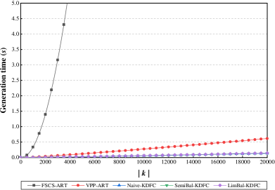
(a) $d=1$

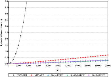
(b) $d=2$

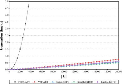
(c) $d=3$

Figure 10: Generation times for various test suite sizes, for $d=1$, $2$, and $3$.

5.3.1 Answer to RQ2 - Part 1: Results of Simulations

Figure 10 shows the test case generation times of VPP-ART, FSCS-ART, and the three KDFC-ART algorithms, for various test suite sizes, in $1$, $2$, and $3-$dimensional input domains. Figure 11 shows the data for $4$, $5$, $8$, and $10-$dimensional input domains. In the figures, the $x$-axis shows the size of the test suite (k), and the $y$-axis shows the time taken to generate the k test cases. Based on the simulation results, we have the following observations:

A. VPP-ART versus FSCS-ART

VPP-ART has a significant advantage over FSCS-ART in terms of test case generation time, across different input domain dimensionalities. Compared with FSCS-ART, VPP-ART uses vantage point partitioning and approximate NN strategies to increase the efficiency. The simulation results indicate that the VPP-ART test case generation time is not obviously impacted by increases in dimensionality: VPP-ART still maintains a strong ability to reduce the time overheads in high dimensions.

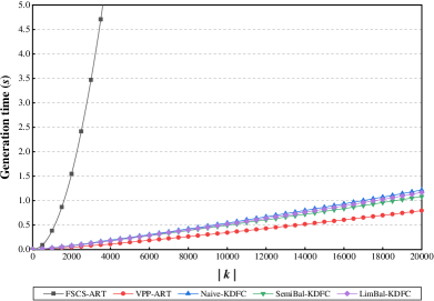
(a) $d=4$

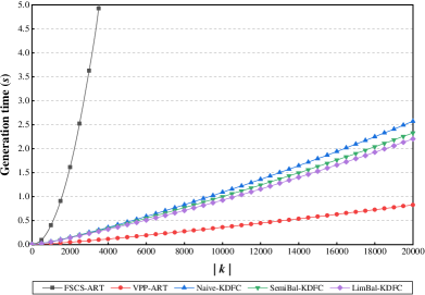
(b) $d=5$

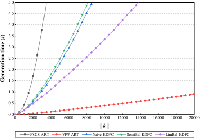
(c) $d=8$

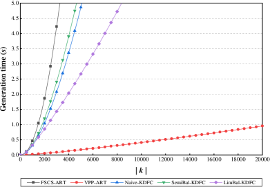
(d) $d=10$

Figure 11: Generation times for various test suite sizes, for $d=4$, $5$, $8$, and $10$.

B. VPP-ART versus KDFC-ART

Figure 10 shows that when $d=1$, $2$, or $3$, there is little difference in test case generation time for the three KDFC-ART versions, all of which have better performance than VPP-ART. Figure 11 shows that when the input domain dimension increases to $d=4$, the KDFC-ART performance becomes worse than VPP-ART. As the dimensionality increases ($d\geq 5$), the performance differences among the three KDFC-ART versions gradually increases, with LimBal-KDFC emerging as the best. However, the performance of all three KDFC-ART versions is worse than that of VPP-ART, with the difference increasing as the dimensionality increases.

Discussion of efficiency simulation results: The simulation results show that VPP-ART requires much less time than FSCS-ART to generate an equal number of test cases. VPP-ART performs slightly worse than KDFC-ART when the dimensionality is low, but increasingly becomes the better performer as the dimensions increase. The two ART algorithms based on approximate NN (LimBal-KDFC and VPP-ART) have better test case generation time. As the number of test cases get larger, the time cost of the approximate NN search is lower than that of the exact NN search.

5.3.2 Answer to RQ2 - Part 2: Results of Experiments

This section reports on the investigation into the efficiency of the five ART algorithms (VPP-ART, FSCS-ART, Naive-KDFC, SemiBal-KDFC, and LimBal-KDFC) on the $22$ subject programs. Table VII reports the average time taken to detect the first failure (F-time) in each program, by each algorithm. Based on the data in the table, the main findings are as follows.

A. VPP-ART versus FSCS-ART

The experiment data show the VPP-ART F-time results to be much lower than those of FSCS-ART: The effect size scores show VPP-ART to be better than FSCS-ART $78\%$ to $93\%$ of the time. The p-values for both algorithms are $0.0000$, which shows a significant difference between VPP-ART and FSCS-ART. In summary, VPP-ART greatly improves on the testing efficiency of FSCS-ART for the real-life subject programs.

TABLE VII: F-times and statistical analysis comparisons among VPP-ART and other different ART algorithms with the $22$ subject programs

No.	Program	Dimension $(d)$	F-time					Statistical Analysis
			VPP- ART	FSCS- ART	Naive- KDFC	SemiBal- KDFC	LimBal- KDFC	vs. FSCS-ART		vs. Naive-KDFC		vs. SemiBal-KDFC		vs. LimBal-KDFC
								p-value	effect size	p-value	effect size	p-value	effect size	p-value	effect size
1	airy	1	12.74	329.08	3.31	3.33	3.71	0.0000	0.8740	0.0000	0.2000	0.0000	0.2008	0.0000	0.2182
2	bessj0	1	6.38	98.95	1.66	1.66	1.76	0.0000	0.8382	0.0000	0.2062	0.0000	0.2061	0.0000	0.2151
3	erfcc	1	17.33	529.69	4.46	4.60	4.80	0.0000	0.8904	0.0000	0.1919	0.0000	0.1971	0.0000	0.2039
4	probks	1	37.18	1081.17	18.11	17.95	18.57	0.0000	0.8845	0.0000	0.3000	0.0000	0.2973	0.0000	0.3057
5	tanh	1	3.98	50.72	1.08	1.17	1.21	0.0000	0.8273	0.0000	0.2044	0.0000	0.2173	0.0000	0.2218
6	bessj	2	7.55	132.59	8.43	3.08	3.97	0.0000	0.7889	0.0000	0.5326	0.0000	0.3214	0.0000	0.3647
7	gammq	2	20.60	775.74	16.10	13.08	14.28	0.0000	0.8319	0.0000	0.4520	0.0000	0.4153	0.0000	0.4330
8	sncndn	2	11.18	287.05	5.53	9.03	9.06	0.0000	0.7967	0.0000	0.3773	0.0000	0.4399	0.0000	0.4528
9	golden	3	45.73	2417.30	45.16	72.10	66.76	0.0000	0.8518	0.1062	0.5120	0.0000	0.5623	0.0000	0.5760
10	plgndr	3	42.52	1714.59	94.44	19.43	21.65	0.0000	0.8155	0.0000	0.6282	0.0000	0.3541	0.0000	0.3745
11	cel	4	36.14	1858.20	155.37	23.46	28.03	0.0000	0.8601	0.0000	0.7358	0.0000	0.4126	0.0000	0.4457
12	el2	4	15.42	379.12	25.32	29.34	28.23	0.0000	0.7910	0.0000	0.5933	0.0000	0.5869	0.0000	0.5968
13	calDay	5	27.57	968.30	169.88	36.91	36.18	0.0000	0.8371	0.0000	0.7733	0.0004	0.5264	0.0088	0.5195
14	complex	6	27.62	1317.92	136.16	136.54	113.95	0.0000	0.8536	0.0000	0.7358	0.0000	0.7446	0.0000	0.7431
15	pntLinePos	6	34.46	1895.50	182.67	193.30	155.95	0.0000	0.8563	0.0000	0.7496	0.0000	0.7640	0.0000	0.7651
16	triangle	6	35.23	1562.98	177.93	180.97	142.86	0.0000	0.8339	0.0000	0.7444	0.0000	0.7453	0.0000	0.7372
17	line	8	102.64	10274.08	1542.17	1659.12	936.30	0.0000	0.8931	0.0000	0.8484	0.0000	0.8432	0.0000	0.8511
18	pntTrianglePos	8	153.93	21846.93	2864.84	3077.41	1450.36	0.0000	0.8972	0.0000	0.8594	0.0000	0.8676	0.0000	0.8547
19	TwoLinesPos	8	272.39	70499.32	6015.84	6919.79	3177.67	0.0000	0.9347	0.0000	0.8831	0.0000	0.8946	0.0000	0.8870
20	nearestDistance	10	69.81	3493.54	3113.37	3467.71	1067.29	0.0000	0.8596	0.0000	0.8503	0.0000	0.8540	0.0000	0.8608
21	calGCD	10	27.96	916.10	483.69	554.96	364.48	0.0000	0.8139	0.0000	0.8033	0.0000	0.8119	0.0000	0.8055
22	select	11	216.93	26894.43	24325.93	23561.25	4338.21	0.0000	0.9035	0.0000	0.9088	0.0000	0.9086	0.0000	0.9039

B. VPP-ART versus KDFC-ART

The results show that when the input domain dimensionality is low, all three KDFC-ART versions require less time than VPP-ART to find the first failure in the subject programs. When $d=1,2$, Naive-KDFC has better performance than VPP-ART, except for the bessj program, but for higher dimensions, according to the effect size scores, VPP-ART outperforms Naive-KDFC approximately $51\%$ to $91\%$ of the time. When $1\leq d\leq 4$, except for the golden and el2 programs, SemiBal-KDFC and LimBal-KDFC outperform VPP-ART. For the other programs/dimensions, VPP-ART outperforms SemiBal-KDFC and LimBal-KDFC in (approximately) $50\%$ to $91\%$, and (approximately) $51\%$ to $91\%$, of the time, respectively. All p-values are less than $0.05$, except for Naive-KDFC’s performance with golden, which shows that the differences in VPP-ART and KDFC-ART performances are significant.

Discussion of efficiency experiments using subject programs: In general, for all subject programs, VPP-ART outperforms FSCS-ART, in terms of the time taken to find the first failure. In low dimensions, KDFC-ART shows better efficiency than VPP-ART, but as the dimensionality increases, VPP-ART outperforms KDFC-ART.

Summary and Discussions of Answers to RQ2: VPP-ART is more efficient than FSCS-ART, according to both the simulation and experimental results. KDFC-ART is more efficient in low-dimensional input domains, but VPP-ART outperforms KDFC-ART when the dimensionality is higher.

Conclusion: Compared with FSCS-ART, the proposed VPP-ART approach not only shows comparable or better failure-detection effectiveness in most cases, but also significantly improves on the FSCS-ART efficiency in most cases. VPP-ART has similar failure-detection effectiveness to KDFC-ART, outperforming KDFC-ART in higher dimensions. VPP-ART, due to the use of vantage point partitioning and the approximate NN search strategy, has the following advantages: (1) VPP-ART can generate an equivalent number of test cases to FSCS-ART in very short time; (2) VPP-ART can find software failures more efficiently than FSCS-ART; and (3) VPP-ART can relieve the influence of dimensionality on the efficiency of KDFC-ART, with VPP-ART not showing performance degradation as the input domain dimensionality increases.

In conclusion, VPP-ART is more cost-effective than FSCS-ART; and in high dimensions, VPP-ART is more cost-effective than KDFC-ART.

6 Threats to Validity

This section examines some potential threats to the validity of our study.

6.1 Construct Validity

Construct validity refers to how well a study examines and measures its assertions. In this paper, we used the F-measure (and related ART F-ratio) [14] to measure the failure-detection effectiveness of RT and different ART algorithms. In addition to the F-measure, two other failure-detection effectiveness metrics that are commonly used are the E-measure and the P-measure [15]. The E-measure refers to the expected number of failures to be identified by a set of test cases; and the P-measure is the probability of a test set identifying at least one program failure. The E-measure and P-measure are most suitable for the evaluation of automated testing systems when the number of test cases is fixed [59]. The F-measure, in contrast, is more suitable when testing continues until a failure is detected. Previous studies have shown that ART outperforms RT in terms of the P-measure [60]. A criticism of the E-measure is that multiple failures may be associated with a single fault [59]. In this paper, we examined FSCS-ART and the enhanced RT algorithms VPP-ART and KDFC-ART in simulations and experiments, with the algorithm stopping whenever a (first) program failure was detected. Accordingly, the F-measure was the metric used to evaluate the failure-finding effectiveness of the three algorithms.

6.2 External Validity

External validity refers to the extent to which our experiments are generally valid, and to what degree can the results and findings be generalized. A potential external threat relates to the existing empirical research (e.g., KDFC-ART [22]). Although the subject programs in our study cover a wide range of failure rates and dimensions, the programs are relatively small in size. To address this threat, our future work will involve more subject programs, including both different types of subject programs (e.g., object-oriented software/systems), and larger-scale programs.

6.3 Internal Validity

Internal validity refers to the accuracy and completeness of the experiments. Each of our experiments was repeated 3000 times, allowing confidence in the calculated average data. Different parameter settings for VPP-ART will lead to different outcomes, which is also a potential threat. For example, we recommended setting the parameter pair values as $\langle\varepsilon,\lambda\rangle=\langle 3,10\rangle$ (Section 5.1): VPP-ART will produce different behavior and results when different parameter values are chosen. As discussed in Section 5.1, a smaller $\lambda$ and a smaller $\varepsilon$ can enhance the VPP-ART performance. However, it is not possible to enumerate every possible parameter value combination.

7 Related Work

Many techniques have been proposed to address the ART computational overhead problem, including: forgetting [20]; Distance-aware Forgetting for Fixed-Size-Candidate-Set ART (DF-FSCS-ART) [21]; KD-tree-enhanced Fixed-Size-Candidate-Set ART (KDFC-ART) [22]; and Fixed-Size-Candidate-Set ART using SIMD instructions (FSCS-SIMD) [23].

7.1 Forgetting

With ART, generation of the next test case depends on the $|E|$ test cases that were already executed, without revealing any failures. As the number of test cases in $E$ grows, the computational overhead of generating test cases becomes greater. Chan et al. [20] proposed a forgetting strategy that only examines up to a constant $M$ number of executed test cases when generating new test cases, typically with $M$ being $\ll|E|$. The forgetting strategy thus makes generation of the next test case independent of the size of $E$. VPP-ART uses the concept of partitioning, with all $|E|$ test cases, but only $\lambda$ test cases are considered in the search process. Both forgetting and VPP-ART can reduce the searching scale of $E$, but there is a difference between the algorithms: The forgetting strategy ignores some executed test cases without considering the relationship between them; with VPP-ART, however, the attribute (distance) information of each test case is indexed by vantage points, thus implicitly including the information when reducing the search scale.

7.2 DF-FSCS-ART

DF-FSCS-ART [21] uses information about the distribution of executed test cases, ignoring those not in the sight of a given candidate test case. The input domain is first divided into $p\times p$ sub-domains (where $p$ is a predefined parameter). During test case generation, FSCS-ART is applied to the entire input domain, but for each candidate test case, only those executed test cases lying in adjacent sub-domains are included in the distance calculation process. When DF-FSCS-ART is dividing the input domain, as long as the division conditions are satisfied, a new round of division will be performed. To avoid too many test cases within the sub-domains, DF-FSCS-ART randomly filters them to keep the number below a threshold value $\lambda$.

DF-FSCS-ART faces some challenges: (1) Two parameters ($p$ and $\lambda$) need to be set before testing, with different values of these two parameters causing the performance of DF-FSCS-ART to vary widely. This is also a threat to our proposed VPP-ART, which requires that the parameter pair $\langle\varepsilon,\lambda\rangle$ be set before testing. (2) As the number of executed test cases increases, more distance calculations need to be performed, increasing the time overheads. Although VPP-ART and DF-FSCS-ART share the same goal of reducing the FSCS-ART computational overheads, the dimensionality and number of executed test cases are significantly stronger limitations for DF-FSCS-ART: As seen in this paper, the VPP-ART time cost changes very little in response to increases in the executed test set size and input domain dimension.

7.3 KDFC-ART

To reduce the high computational overheads of FSCS-ART, Mao et al. [22] proposed three KDFC-ART algorithms, based on the K-dimensional tree (KD-tree) [61, 62, 63, 64] structure: Naive-KDFC; SemiBal-KDFC; and LimBal-KDFC. Naive-KDFC sequentially divides the input space in each dimension to construct the KD-tree. To improve the balance of the KD-tree, SemiBal-KDFC prioritizes the partitioning using a splitting strategy [22] Because the KD-tree structure has a drawback that, in the worst case (especially when the dimensionality increases), all nodes may need to be traversed, the third algorithm, LimBal-KDFC, was proposed: LimBal-KDFC uses an upper limit to control the number of traversed nodes in the backtracking. Naive-KDFC and SemiBal-KDFC are based on an exact NN search; while LimBal-KDFC uses on approximate NN search — the same as VPP-ART. As shown in this paper, both VPP-ART and KDFC-ART focus on reducing the high computational overheads of ART, and each has its own advantages and disadvantages. VPP-ART shows the improvement in high-dimensional efficiency due to its use of the VPP for distances among test cases: VPP-ART test case generation time changes little as the dimensionality increases.

7.4 FSCS-SIMD

Ashfaq et al. [23] proposed an efficient FSCS-ART implementation, Fixed-Size-Candidate-Set using Single-Instruction-Multiple-Data (FSCS-SIMD), which uses the SIMD instruction architecture to calculate the distances among multiple test cases simultaneously, in a many-to-many manner. FSCS-SIMD loads a batch of multiple test cases from the candidate and executed test case sets at once. FSCS-SIMD accelerates the distance computation by increasing the CPU execution utilization, but is dependent on the available hardware resources [23]. VPP-ART, in contrast, improves the efficiency at the level of the algorithm and data structures. In poorer hardware environments (such as with a low number of CPU cores), FSCS-SIMD has greater limitations than VPP-ART because FSCS-SIMD depends more on the hardware resources.

8 Conclusions and Future Work

Adaptive Random Testing (ART) [13] improves on the failure-detection effectiveness of Random Testing (RT) [6], by making the test cases more evenly distributed in the input domain. The Fixed-Size-Candidate-Set ART (FSCS-ART) [13] was among the first ART implementations, and has remained among the most popular [12]: FSCS-ART is widely used in practice, and has been shown to have better failure-detection effectiveness [13, 14, 15, 16], test-case distribution [17], and code coverage [18] than RT. However, FSCS-ART still has a significant computational overhead problem [12]: The time required to generate/select FSCS-ART test cases is much greater than their execution time. In this paper, we have proposed the VPP-ART algorithm, which make use of Vantage Point Partitioning (VPP) and an approximate nearest neighbor (NN) search strategy. VPP-ART achieves a significant reduction in the time overheads for FSCS-ART while maintaining its effectiveness.

We conducted a series of simulations and experimental studies to validate the VPP-ART approach, using FSCS-ART and three KDFC-ART algorithms for comparison. The simulations showed that VPP-ART not only requires less time to detect software failures compared with FSCS-ART, but also retains comparable failure-detection effectiveness. VPP-ART also has similar, or better, failure-detection effectiveness compared with KDFC-ART [22]. In terms of efficiency, KDFC-ART has lower overheads in low dimensions, but VPP-ART performs better in high dimensions. Furthermore, the VPP-ART time overheads only increase slightly for increases in the input domain dimensionality. VPP-ART effectively reduces the computational overhead problem of FSCS-ART, and is cost-effective.

The ART algorithms based on exact NN searches have better failure-detection effectiveness in lower dimensional input domains, while those based on approximate NN are better in higher dimensions. This is because of the clustering of similar test cases, which is more pronounced as the dimensionality and number of test cases increases, resulting in more similar test cases clustering in the same sub-domain. Moreover, when there is little difference between the approximate and the exact NNs, the approximate NN can replace the exact NN, improving the search efficiency (test case generation efficiency) at the cost of a tolerable loss in accuracy.

In this paper, we introduced a modified VP-tree to support the dynamic nature of FSCS-ART. Because many other ART approaches and implementations also suffer from the same drawbacks and overheads as FSCS-ART, our future work will include exploration of application of the insert-able VP-tree to these other ART algorithms. Furthermore, as mentioned in the Threats to Validity section (Section 6), confirmation of the VPP-ART parameter settings for $\lambda$ and $\varepsilon$ is also one of the future research directions. The influence of the parameter pairs ($\lambda$ and $\varepsilon$) on the effectiveness of the experiments has been discussed, with the experimental parameter pair values determined from the simulations. However, because there has not yet been much research into these two parameters, exploring the functional or dependency relationship between them, so that our proposed insert-able VP-tree structure can be better applied, will also form part of our future work. VPP-ART is an ART algorithm based on an approximate NN search (like LimBal-KDFC): Our experimental analysis has shown that VPP-ART and LimBal-KDFC can effectively improve on the high dimensional failure-detection effectiveness of the original ART algorithm, and greatly reduce the test case generation time. This gives us some inspiration to identify and create other algorithms or data structures that may be enhanced through an approximate, rather than exact, NN search.

References

- [1] S. Anand, E. K. Burke, T. Y. Chen, J. A. Clark, M. B. Cohen, W. Grieskamp, M. Harman, M. J. Harrold, and P. McMinn, “An orchestrated survey of methodologies for automated software test case generation,” Journal of Systems and Software, vol. 86, no. 8, pp. 1978–2001, 2013.
- [2] A. Orso and G. Rothermel, “Software testing: A research travelogue (2000-2014),” in Proceedings of Future of Software Engineering (FOSE’14), 2014, pp. 117–132.
- [3] E. J. Weyuker, “On testing non-testable programs,” The Computer Journal, vol. 25, no. 4, pp. 465–470, 1982.
- [4] E. T. Barr, M. Harman, P. McMinn, M. Shahbaz, and S. Yoo, “The oracle problem in software testing: A survey,” IEEE Transactions on Software Engineering, vol. 41, no. 5, pp. 507–525, 2015.
- [5] G. Jahangirova, “Oracle problem in software testing,” in Proceedings of the 26th ACM SIGSOFT International Symposium on Software Testing and Analysis (ISSTA’17), 2017, pp. 444–447.
- [6] A. Arcuri, M. Iqbal, and L. Briand, “Random testing: Theoretical results and practical implications,” IEEE Transactions on Software Engineering, vol. 38, no. 2, pp. 258–277, 2012.
- [7] B. K. Ozkan, R. Majumdar, F. Niksic, M. T. Befrouei, and G. Weissenbacher, “Randomized testing of distributed systems with probabilistic guarantees,” Proceedings of the Acm on Programming Languages, vol. 2, no. OOPSLA, pp. 160:1–160:28, 2018.
- [8] V. Livinskii, D. Babokin, and J. Regehr, “Random testing for C and C++ compilers with yarpgen,” Proceedings of the Acm on Programming Languages, vol. 4, no. OOPSLA, pp. 196:1–196:25, 2020.
- [9] T. D. White, G. Fraser, and G. J. Brown, “Improving random GUI testing with image-based widget detection,” in Proceedings of the 28th ACM SIGSOFT International Symposium on Software Testing and Analysis, (ISSTA’19), 2019, pp. 307–317.
- [10] H. Pei, K. Cai, B. Yin, A. P. Mathur, and M. Xie, “Dynamic random testing: Technique and experimental evaluation,” IEEE Transactions on Reliability, vol. 68, no. 3, pp. 872–892, 2019.
- [11] H. Pei, B. Yin, M. Xie, and K. Cai, “Dynamic random testing with test case clustering and distance-based parameter adjustment,” Information and Software Technology, vol. 131, p. 106470, 2021.
- [12] R. Huang, W. Sun, Y. Xu, H. Chen, D. Towey, and X. Xia, “A survey on adaptive random testing,” IEEE Transactions on Software Engineering, vol. 47, no. 10, pp. 2052–2083, 2021.
- [13] T. Y. Chen, H. Leung, and I. K. Mak, “Adaptive random testing,” in Proceedings of the 9th Asian Computing Science Conference (ASIAN’04), 2004, pp. 320–329.
- [14] T. Y. Chen, F.-C. Kuo, and R. G. Merkel, “On the statistical properties of the F-measure,” in Proceedings of the 4th International Conference on Quality Software (QSIC’04), 2004, pp. 146–153.
- [15] T. Y. Chen, F. Kuo, and R. G. Merkel, “On the statistical properties of testing effectiveness measures,” Journal of Systems and Software, vol. 79, no. 5, pp. 591–601, 2006.
- [16] T. Y. Chen, F.-C. Kuo, and Z. Q. Zhou, “On favourable conditions for adaptive random testing,” International Journal of Software Engineering and Knowledge Engineering, vol. 17, no. 06, pp. 805–825, 2007.
- [17] T. Y. Chen, F.-C. Kuo, and H. Liu, “On test case distributions of adaptive random testing,” in Proceedings of the 19th International Conference on Software Engineering and Knowledge Engineering (SEKE’07), 2007, pp. 141–144.
- [18] T. Y. Chen, F.-C. Kuo, H. Liu, and W. E. Wong, “Code coverage of adaptive random testing,” IEEE Transactions on Reliability, vol. 62, no. 1, pp. 226–237, 2013.
- [19] H. Wu, C. Nie, J. Petke, Y. Jia, and M. Harman, “An empirical comparison of combinatorial testing, random testing and adaptive random testing,” IEEE Transactions on Software Engineering, vol. 46, no. 3, pp. 302–320, 2020.
- [20] K.-P. Chan, T. Y. Chen, and D. Towey, “Forgetting test cases,” in Proceedings of the 30th Annual International Computer Software and Applications Conference (COMPSAC’06), 2006, pp. 485–494.
- [21] C. Mao, T. Y. Chen, and F.-C. Kuo, “Out of sight, out of mind: a distance-aware forgetting strategy for adaptive random testing,” Science China Information Sciences, vol. 60, no. 9, pp. 092 106:1–092 106:21, 2017.
- [22] C. Mao, X. Zhan, T. H. Tse, and T. Y. Chen, “KDFC-ART: a KD-tree approach to enhancing Fixed-size-Candidate-set Adaptive Random Testing,” IEEE Transactions on Reliability, vol. 68, no. 4, pp. 1444–1469, 2019.
- [23] M. Ashfaq, R. Huang, and M. Omari, “FSCS-SIMD: an efficient implementation of fixed-size-candidate-set adaptive random testing using SIMD instructions,” in Proceedings of 31st IEEE International Symposium on Software Reliability Engineering (ISSRE’20), 2020, pp. 277–288.
- [24] C. Chow, T. Y. Chen, and T. Tse, “The ART of divide and conquer: An innovative approach to improving the efficiency of adaptive random testing,” in Proceedings of the 13th International Conference on Quality Software (QSIC’13), 2013, pp. 268–275.
- [25] R. Huang, H. Liu, X. Xie, and J. Chen, “Enhancing mirror adaptive random testing through dynamic partitioning,” Information and Software Technology, vol. 67, pp. 13–29, 2015.
- [26] T. Y. Chen, F.-C. Kuo, R. Merkel, and S. P. Ng, “Mirror adaptive random testing,” Information and Software Technology, vol. 46, no. 15, pp. 1001–1010, 2004.
- [27] P. N. Yianilos, “Data structures and algorithms for nearest neighbor search in general metric spaces,” in Proceedings of the Fourth Annual ACM/SIGACT-SIAM Symposium on Discrete Algorithms (SODA’93), 1993, pp. 311–321.
- [28] J. K. Uhlmann, “Satisfying general proximity/similarity queries with metric trees,” Information Processing Letters, vol. 40, no. 4, pp. 175–179, 1991.
- [29] T. Chiueh, “Content-based image indexing,” in Proceedings of 20th International Conference on Very Large Data Bases (VLDB’94), J. B. Bocca, M. Jarke, and C. Zaniolo, Eds., 1994, pp. 582–593.
- [30] L. White and E. Cohen, “A domain strategy for computer program testing,” IEEE Transactions on Software Engineering, vol. 6, no. 3, pp. 247–257, 1980.
- [31] P. E. Ammann and J. C. Knight, “Data diversity: An approach to software fault tolerance,” IEEE Transactions on Computers, vol. 37, no. 4, pp. 418–425, 1988.
- [32] G. B. Finelli, “Nasa software failure characterization experiments,” Reliability Engineering and System Safety, vol. 32, no. 1–2, pp. 155–169, 1991.
- [33] P. G. Bishop, “The variation of software survival times for different operational input profiles,” in Prceedings of the 23rd International Symposium on Fault-Tolerant Computing (FTCS’93), 1993, pp. 98–107.
- [34] C. Schneckenburger and J. Mayer, “Towards the determination of typical failure patterns,” in Proceedings of the 4th International Workshop on Software Quality Assurance (SOQUA’07), 2007, pp. 90–93.
- [35] F. Chan, T. Y. Chen, I. Mak, and Y.-T. Yu, “Proportional sampling strategy: Guidelines for software testing practitioners,” Information and Software Technology, vol. 38, no. 12, pp. 775–782, 1996.
- [36] J. S. Sánchez, J. M. Sotoca, and F. Pla, “Efficient nearest neighbor classification with data reduction and fast search algorithms,” in Proceedings of the IEEE International Conference on Systems, Man & Cybernetics (SMC’04), 2004, pp. 4757–4762.
- [37] T. DeFreitas, H. Saddiki, and P. Flaherty, “GEMINI: a computationally-efficient search engine for large gene expression datasets,” BMC Bioinformatics, vol. 17, p. 102, 2016.
- [38] I. Markov, “Vp-tree: Content-based image indexing,” in Proceedings of the SYRCoDIS 2007 Colloquium on Databases and Information Systems (SYRCoDIS’07), vol. 256, 2007.
- [39] M. Shishibori, Samuel Sangkon Lee, and K. Kita, “A method to improve metric index vp-tree for multimedia databases,” in 2011 17th Korea-Japan Joint Workshop on Frontiers of Computer Vision (FCV’11), 2011, pp. 1–6.
- [40] M. Skalak, J. Han, and B. Pardo, “Speeding melody search with vantage point trees,” in 9th International Conference on Music Information Retrieval (ISMIR’08), 2008, pp. 95–100.
- [41] N. Kumar, L. Zhang, and S. K. Nayar, “What is a good nearest neighbors algorithm for finding similar patches in images?” in 10th European Conference on Computer Vision (ECCV’08), vol. 5303, 2008, pp. 364–378.
- [42] A. W. Fu, P. M. Chan, Y. Cheung, and Y. S. Moon, “Dynamic vp-tree indexing for n-nearest neighbor search given pair-wise distances,” VLDB Journal, vol. 9, no. 2, pp. 154–173, 2000.
- [43] T. Y. Chen, D. H. Huang, and Z. Q. Zhou, “Adaptive random testing through iterative partitioning,” in Proceedings of the 11th Ada-Europe International Conference on Reliable Software Technologies (Ada-Europe’06), 2006, pp. 155–166.
- [44] N. L. Leech and A. J. Onwuegbuzie, “A call for greater use of nonparametric statistics,” Classification, 2002.
- [45] R. J. Grissom and J. J. Kim, Effect sizes for research: A broad practical approach. Lawrence Erlbaum Associates Publishers, 2005.
- [46] A. Arcuri and L. Briand, “A hitchhiker’s guide to statistical tests for assessing randomized algorithms in software engineering,” Software Testing, Verification and Reliability, vol. 24, no. 3, pp. 219–250, 2014.
- [47] T. Menzies, S. Williams, B. W. Boehm, and J. Hihn, “How to avoid drastic software process change (using stochastic stability),” in Proceedings of the 31st International Conference on Software Engineering (ICSE’09), 2009, pp. 540–550.
- [48] M. Cowles and C. Davis, “On the origins of the. 05 level of statistical significance,” American Psychologist, vol. 37, no. 5, p. 553, 1982.
- [49] A. Vargha and H. D. Delaney, “A critique and improvment of the CL common language effect size statistics of mcgraw and wong,” Journal of Education and Behavioral Statistics, vol. 25, no. 2, pp. 101–132, 2000.
- [50] Y. Jia and M. Harman, “An analysis and survey of the development of mutation testing,” IEEE Transactions on Software Engineering, vol. 37, no. 5, pp. 649–678, 2010.
- [51] T. Y. Chen and F. Kuo, “Is adaptive random testing really better than random testing,” in Proceedings of the 1st International Workshop on Random Testing (RT’06), 2006, pp. 64–69.
- [52] T.-Y. Chen, F.-C. Kuo, and C.-A. Sun, “Impact of the compactness of failure regions on the performance of adaptive random testing,” Journal of Software, vol. 17, pp. 2438–2449, 2006.
- [53] W. Press, B. P. Flannery, S. A. Teulolsky, and W. T. Vetterling, Numerical Recipes. Cambridge University Press: Cambridge, 1986.
- [54] ACM, Collected Algorithms from ACM. Association for Computer Machinery: New York, 1980.
- [55] K. P. Chan, T. Y. Chen, and D. Towey, “Restricted random testing: Adaptive random testing by exclusion,” International Journal of Software Engineering and Knowledge Engineering, vol. 16, no. 4, pp. 553–584, 2006.
- [56] J. Ferrer, F. Chicano, and E. Alba, “Evolutionary algorithms for the multi-objective test data generation problem,” Software: Practice and Experience, vol. 42, no. 11, pp. 1331–1362, 2012.
- [57] Y. D. Liang, “Introduction to java programming and data structures,” Comprehensive Version, 11th ed. London, UK: Pearson Education, 2017.
- [58] P. S. May, “Test data generation : two evolutionary approaches to mutation testing,” Ph.D. dissertation, University of Kent, Canterbury, UK, 2007.
- [59] A. Shahbazi, A. F. Tappenden, and J. Miller, “Centroidal Voronoi Tessellations - A new approach to random testing,” IEEE Transactions on Software Engineering, vol. 39, no. 2, pp. 163–183, 2013.
- [60] T. Y. Chen, D. H. Huang, T. H. Tse, and Z. Yang, “An innovative approach to tackling the boundary effect in adaptive random testing,” in Proceedings of the 40th Annual Hawaii International Conference on System Sciences (HICSS’07), 2007, pp. 262a–262a.
- [61] J. L. Bentley, “Multidimensional binary search trees used for associative searching,” Communications of the ACM, vol. 18, no. 9, pp. 509–517, 1975.
- [62] J. Kubica, J. Masiero, A. W. Moore, R. Jedicke, and A. J. Connolly, “Variable KD-tree algorithms for spatial pattern search and discovery,” in Advances in Neural Information Processing Systems 18 Neural Information Processing Systems (NIPS’05), 2005, pp. 691–698.
- [63] A. Adams, N. Gelfand, J. Dolson, and M. Levoy, “Gaussian KD-trees for fast high-dimensional filtering,” ACM Transactions on Graphics, vol. 28, no. 3, p. 21, 2009.
- [64] T. Foley and J. Sugerman, “KD-tree acceleration structures for a GPU raytracer,” in Proceedings of the ACM SIGGRAPH/EUROGRAPHICS Symposium on Graphics Hardware (GH’05), 2005, pp. 15–22.