Conservation-law-based global bounds to quantum optimal control

Abstract

Active control of quantum systems enables diverse applications ranging from quantum computation to manipulation of molecular processes. Maximum speeds and related bounds have been identified from uncertainty principles and related inequalities, but such bounds utilize only coarse system information, and loosen significantly in the presence of constraints and complex interaction dynamics. We show that an integral-equation-based formulation of conservation laws in quantum dynamics leads to a systematic framework for identifying fundamental limits to any quantum control scenario. We demonstrate the utility of our bounds in three scenarios—three-level driving, decoherence suppression, and maximum-fidelity gate implementations—and show that in each case our bounds are tight or nearly so. Global bounds complement local-optimization-based designs, illuminating performance levels that may be possible as well as those that cannot be surpassed.

In this Letter, we develop a framework for computing fundamental limits to what is possible via control of quantum systems. We show that quantum control problems can be transformed to quadratically constrained quadratic programs (QCQPs), with generalized probability conservation laws as the constraints, adapting a mathematical approach recently developed for light–matter interactions [1, 2]. The QCQP formulation enables global bounds via relaxations to semidefinite programs [3, 4]. We demonstrate the power and utility of our method on three prototype systems: (1) three-level system driving, where our bounds incorporate sophisticated information about interference between levels, and can account for constraints on undesirable transitions (as needed in transmons [5], for example), (2) upper bounds to the suppression of decoherence, and (3) the maximum fidelity of a control-based implementation of a single-qubit Hadamard gate. In each case we supplement our bounds with many local-optimization-based solutions, showing that they come quite close to (and in some cases achieve) our bounds, suggesting that our bounds are tight or nearly so. Our framework applies to open and closed systems, can be extended to related domains in NMR [6, 7, 8] and quantum complexity [9, 10, 11], and should reveal the limits of what is possible with quantum control.

Quantum control [12, 13, 14, 15, 16] refers to the design and synthesis of efficient control sequences that drive a quantum system to maximize a desired objective, such as maximizing overlap with a target state or minimizing error in the implementation of a gate operation. Recent experiments have demonstrated the power of optimal control for wide-ranging applications [17, 18, 19, 20, 21, 22]. Because the wave function $\ket{\psi(t)}$ that represents a quantum state is nonlinear in the control parameter $\varepsilon(t)$, it is generically difficult to identify globally optimal controls. One strategy is to use local numerical optimization over the control parameters (e.g. GRAPE [6, 23, 24, 25], the Krotov method [26, 27, 28, 29, 30, 31], and CRAB [32, 33]), optimizing over many initial conditions in the hopes of identifying high-performance local optima. Yet, except in the simplest of systems, one is left uncertain about the best performance possible. Alternatively, there are a variety of global bounds [34, 35, 36, 37, 38, 39, 40, 41, 42, 43, 44, 45, 46, 47, 48, 49, 50, 51, 52, 53, 54, 55]; most famously, the Mandelstam–Tamm (MT) bound. The MT bound is a prototype of “quantum speed limits,” which more generally have varying levels of complexity but are essentially time-energy uncertainty relations [34, 35, 36, 37, 40, 44, 45, 52, 53, 54, 55, 56]. The energy measure is typically a matrix norm of the Hamiltonian, but more complex details of the system interactions are not captured. Another class of bounds is obtained by analytically solving Pontryagin’s maximum principle [57], which is only possible in simple cases such as two-level systems [38, 39, 42, 43, 46, 47, 48]. Consequently, meaningful, accurate bounds cannot be computed for most quantum control systems of interest.

Formulation—We consider a Hamiltonian of the form $H_{0}(t)+H_{c}^{\prime}(t)=H_{0}(t)+\varepsilon(t)H_{c}(t)$, where $H_{0}$ is the non-controllable part of the Hamiltonian, $H_{c}^{\prime}$ is the controllable part, and $\varepsilon$ is the control parameter to be optimized. We assume the control parameter is bounded between 0 and $\varepsilon_{\rm max}$ (any other minimum value can be shifted to 0 by replacing $H_{0}$ with $H_{0}+\varepsilon_{\rm min}H_{c}$). Our method generalizes to any number of control parameters (cf. SM), but for simplicity we assume one throughout this paper. Any smooth, continuous, bounded control can be approximated with arbitrary accuracy by a “bang–bang” binary control that only takes the values 0 and $\varepsilon_{\rm max}$ (cf. SM), so we use bang–bang controls in our formulation. Instead of the differential Schrödinger equation for the time-evolution operator $U(t,t_{0})$ (for an initial time $t_{0}$), we instead start with an integral form (equivalent to the Dyson equation [58, 59] in the interaction picture):

$$U(t,t_{0})=U_{0}(t,t_{0})-\frac{i}{\hbar}\int_{t_{0}}^{T}G_{0}^{+}(t,t^{\prime})H_{c}^{\prime}(t^{\prime})U(t^{\prime},t_{0}){\color[rgb]{0,0,0}\,{\rm d}{t}^{\prime}},$$ (1)

where $U_{0}$ and $G_{0}^{+}$ are the time-evolution operator and retarded Green’s function in the absence of controls (i.e., for $H_{0}(t)$), and $T$ is the final time. To derive conservation laws, we start by taking the product of Eq. (1) with $U^{\dagger}(t,t_{0})H_{c}^{\prime}(t)D_{i}(t)$ from the left and integrating from an initial time $t_{0}$ to $T$:

$$\int_{t_{0}}^{T}U^{\dagger}(t,t_{0})H_{c}^{\prime}(t)D_{i}(t)U(t,t_{0})\,{\rm d}{t}$$

$$+\frac{i}{\hbar}\int_{t_{0}}^{T}\int_{t_{0}}^{T}U^{\dagger}(t,t_{0})H_{c}^{\prime}(t)D_{i}(t)G_{0}^{+}(t,t^{\prime})H_{c}^{\prime}(t^{\prime})U(t^{\prime},t_{0})\,{\rm d}{t}\,{\rm d}{t^{\prime}}$$

$$=\int_{t_{0}}^{T}U^{\dagger}(t,t_{0})H_{c}^{\prime}(t)D_{i}(t)U_{0}(t,t_{0})\,{\rm d}{t}.$$ (2)

The variable $D_{i}(t)$ can be any time-dependent operator and is an optimization hyperparameter below in Eq. (5); intuitively, allowing different possible choices of $D_{i}$ enables the isolation of particular times and elements in Hilbert space for which Eq. (2) should be satisfied. The variable $H_{c}$ is effectively a renormalization that simplifies the probabilistic interpretation below; equivalently, it can be omitted. The constraint of Eq. (2) depends on both the time-evolution degrees of freedom $U(t)$ and the control variable degrees of freedom $\varepsilon(t)$. However, if we define a new variable $\Phi(t)=\varepsilon(t)H_{c}(t)U(t,t_{0})$, this variable (the analog of a polarization field in electrodynamics [60, 1]) can subsume both. Crucially, we can replace any instance of $\varepsilon(t)$ with $\varepsilon_{\rm max}$. This can be thought of as a two-step simplification: one could restrict the domains of the integrals to only times in which the control is on, in which case such a replacement is trivial. Next, $\varepsilon(t)$ only appears in a term of the form $\Phi^{\dagger}\varepsilon^{-1}\Phi$, which is zero even when $\varepsilon(t)=0$, due to the quadratic dependence on $\Phi$. Hence we can extend the domain of the integrals back to the entire time interval from $t_{0}$ to $T$. Such “domain-obliviousness” [1] arises from our inclusion of $\varepsilon(t)$ and $U^{\dagger}(t,t_{0})$ in the product term. Finally, we have the constraints:

$$\int_{t_{0}}^{T}\!\int_{t_{0}}^{T}\!\Phi^{\dagger}(t)D_{i}(t)\!\left[\frac{H_{c}^{-1}(t)}{\varepsilon_{\rm max}}\delta(t-t^{\prime})\!+\!\frac{i}{\hbar}G_{0}^{+}(t,t^{\prime})\right]\!\Phi(t^{\prime}){\color[rgb]{0,0,0}\mathrm{d}t\,\mathrm{d}t^{\prime}}$$

$$=\int_{t_{0}}^{T}\Phi^{\dagger}(t)D_{i}(t)U_{0}(t,t_{0})\,{\rm d}{t},$$ (3)

where $H_{c}^{-1}$ is taken to be the pseudo inverse if $H_{c}$ is not invertible. For any $D_{i}(t)$, Eq. (3) is a quadratic equation in the variable $\Phi(t)$; the set of all possible $D_{i}(t)$ imply an infinite number of quadratic constraints.

Equation (3) can be interpreted as a generalization of probability conservation. At any time $t_{1}$, conservation of probability implies unitarity of the time-evolution operator $U(t_{1},t_{0})$, such that $U^{\dagger}U=\mathcal{I}$, where $\mathcal{I}$ is the identity operator. From the integral equation for $U$, Eq. (1), the difference $U^{\dagger}U-\mathcal{I}$ can be written

$$U^{\dagger}(t_{1},t_{0})U(t_{1},t_{0})-\mathcal{I}$$

$$=\frac{1}{\hbar^{2}}\int_{t_{0}}^{t_{1}}\int_{t_{0}}^{t_{1}}\Phi^{\dagger}(t^{\prime\prime},t_{0})U_{0}(t^{\prime\prime},t^{\prime})\Phi(t^{\prime},t_{0})\,{\rm d}{t^{\prime}}\,{\rm d}{t^{\prime\prime}}$$

$$+\frac{2}{\hbar}\operatorname{Im}\int_{t_{0}}^{t_{1}}U_{0}(t_{0},t^{\prime})\Phi(t^{\prime},t_{0})\,{\rm d}{t^{\prime}}.$$ (4)

If we take the imaginary part of Eq. (3), and choose $D_{i}(t)$ to be the identity operator from $t_{0}$ to $t_{1}$ (and zero otherwise), the resulting constraint is precisely the one that requires the right-hand side of Eq. (4) to be zero (cf. SM). In other words, a subset of the constraints of Eq. (3) are those which enforce unitary evolution at all times. (In an open system described by a density matrix, unitarity is not preserved and the corresponding constraints instead represent conservation of probability flow, cf. SM.)

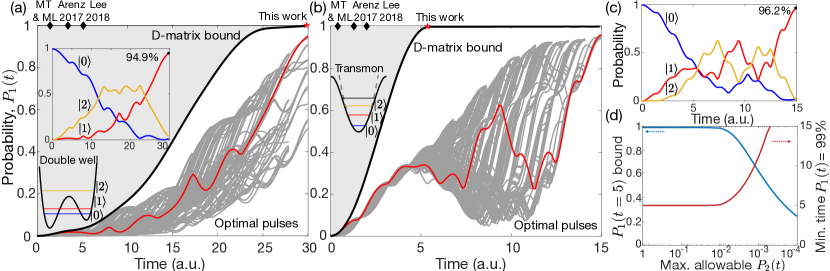
Figure 1: (a) Bounds on the maximum probability in state $\ket{1}$ as a function of time (solid black) for an asymmetric double-well potential, with shading above to indicate impossible values. Grey lines represent pulse evolutions optimized by gradient ascent, with the red line the very best evolution for final time 30. Inset: evolution of probabilities in states $\ket{0},\ket{1},\ket{2}$ for the optimal control, showing the complex dynamics captured by the bound. Black diamonds: evaluations of bounds of Mandelstam–Tamm, Margolus–Levitin, and Refs. [54, 55] for this problem. (b,c) Analogous to (a) but for a three-level model of a transmon qubit. (d) Incorporation of an additional constraint requiring small maximum allowable excitation probabilities of state 2. The bound on the maximum state-$\ket{1}$ probability (at time 5) decreases accordingly. The time to achieve $99\%$ state-$\ket{1}$ probability increases substantially with smaller allowed leakage rates.

Although our derivation implies only that the conservation laws of Eq. (3) are necessary conditions for describing quantum evolution, one can show that they are sufficient as well: any $\Phi(t)$ that satisfies all possible versions of Eq. (3) implies a corresponding time-evolution operator $U(t,t_{0})$ that satisfies Eq. (1) (cf. SM, [61]). Hence, we can replace the differential or integral dynamical equations with the conservation-law constraints of Eq. (3). The optimal-control problem, for any objective $f$ that is a linear or quadratic function of the time-evolution operator $U$, and therefore a linear or quadratic function of $\Phi=\varepsilon H_{c}U$, is then the QCQP:

$$\underset{\Phi}{\text{max.}} f(\Phi)$$ (5)

s.t. $$\textrm{Equation~{}(\ref{eq:Dconstr}) satisfied for all }D_{i}(t).$$

We assume the problem has been discretized in any standard basis [62]. If we denote $\bm{\Phi}$ to be a single column vector containing the full discretization of $\Phi(t)$, Eq. (5) is a maximization of an objective of the form $\bm{\Phi}^{\dagger}A\bm{\Phi}+\operatorname{Re}(\bm{\alpha}^{\dagger}\bm{\Phi})$, where $A$ is Hermitian, subject to constraints of the form $\bm{\Phi}^{\dagger}B_{i}\bm{\Phi}+\operatorname{Re}(\bm{\beta}^{\dagger}_{i}\bm{\Phi})=0$ for all $i$. QCQPs are generically NP-hard to solve, but bounds on their solutions can be computed efficiently after semidefinite relaxation (SDR). SDRs transform quadratic forms $\Phi^{\dagger}A\Phi$ to equivalent linear forms $\Tr{AX}$, where $X$ is a rank-one positive semidefinite matrix, then drop the rank-one constraint. Finally, we are left with an objective of the form $\Tr{AX}+\operatorname{Re}(\bm{\alpha}^{\dagger}\bm{\Phi})$ subject to the constraints that $\Tr{B_{i}X}+\operatorname{Re}(\bm{\beta}_{i}^{\dagger}\bm{\Phi})=0$ for all $i$ and $X\succeq 0$, which is a semidefinite program whose global optimum can be computed via interior-point methods [63, 4]. As the bounds are computed over all possible matrices $D_{i}$, we label them “D-matrix bounds.” This framework applies broadly across quantum control; next, we demonstrate bounds for three prototypical systems.

Applications—First, we compute bounds on driving three-level quantum systems. We consider two three-level systems described by Hamiltonians $H=\hbar\sum_{{\color[rgb]{0,0,0}i}=1,2}\omega_{j}\outerproduct{i}{i}-\varepsilon(t)\sum_{i,j=0,1,2}\mu_{ij}\outerproduct{i}{j}$: one modeling an asymmetric double-well potential, with exact parameters from Sec. 2.8 of [13] and given in the SM, and a second modeling a weakly nonlinear harmonic oscillator with nearest-level couplings, as is typically used to model a transmon qubit [5, 64]. (We consider both systems as they have different features: the first, couplings between all levels, and the second, small anharmonicity with hard-to-avoid leakage.) In each case we assume the system starts in the ground state, $\ket{0}$, and that we want to drive it to the first excited state, $\ket{1}$, as rapidly as possible. We denote the probability of occupying state $i$ at time $t$ by $P_{i}(t)=\left|\innerproduct{i}{\psi(t)}\right|^{2}$. There are two classes of bounds that we can compute: for a given amount of time $T$, the maximum probability in $\ket{1}$, $P_{1}(t)$; or, iteratively, the minimum amount of time to achieve near-unity probability in $\ket{1}$.

The black curve of Fig. 1(a) is the computed bound on $P_{1}(t)$ for the asymmetric-double-well model, for a bounded control field with $|\varepsilon(t)|\leq 0.15$. The shaded region of the figure is impossible to reach: our bounds indicate that any such evolution would necessarily violate at least one of the conservation laws. The grey lines are the results of local computational optimizations; we implemented a gradient-ascent optimization (similar to GRAPE) as described in the SM, for many different final times and initial pulse sequences. The gap between the local optimizations and the bounds arises from two sources—looseness in the bounds (from the SDR) or insufficient local exploration of the optimal pulses—though it is hard to pinpoint which source is more responsible. Also included in the figure are data points corresponding to evaluations of other bounds as applied to this problem: Mandelstam–Tamm (MT), Margolus–Levitin (ML), and Refs. [54, 55]. It takes some effort to map the various bounds to this problem, with varying degrees of looseness, which we discuss in detail in the SM. In particular, however, one can see that each of these bounds predicts minimal times an order of magnitude smaller than our approach. The inset provides a likely explanation: the optimal trajectory (highlighted in red) first populates the second excited state, then transitions to the first excited state through appropriate driving. Such complex dynamics cannot be captured by any previous bound approaches, but can be captured by our approach.

Parts (b–d) of Fig. 1 show results for the transmon-qubit model, with $\omega_{1}=0.19$, $\omega_{2}=0.37$, $\mu_{10}=\mu_{01}=-1$, $\mu_{21}=\mu_{12}=-\sqrt{2}$ (all other $\mu_{ij}=0$), and $|\varepsilon(t)|\leq 0.3$. Fig. 1(b,c) are the transmon analogs of Fig. 1(a). The key novelty that is possible in this case is the addition of a constraint on the excitation probability of the second excited state, $\ket{2}$. Such “leakage” can be highly detrimental to the practical control of such systems, as they can open up additional decoherence channels [65]. In our approach, we can simply add to Eq. (5) a (quadratic) constraint on the maximum allowed probability in $\ket{2}$. In Fig. 1(d), we show the bound for maximum $P_{1}(t)$ subject to varying constraints on the maximum allowed $P_{2}(t)$, at time $t=5$, which shows the dramatic reduction that is required if state-$\ket{2}$ transitions are to be avoided. Conversely, also in Fig. 1(d), the minimum time for near-unity first-state probability increases dramatically with more stringent constraints (red). Such constraints could not be incorporated into previous bound approaches.

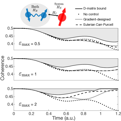
Figure 2: For a spin system interacting with a spin bath, the D-matrix approach enables bounds on maximum possible coherence as a function of time. The black solid line bounds the magnitude of the off-diagonal element of the system density matrix, $\left|\rho^{S}_{12}\right|$, for varying maximum control amplitudes $\varepsilon_{\rm max}$. The time evolutions of $\left|\rho^{S}_{12}\right|$ for pulses designed by gradient-ascent (solid grey) and finite Carr-Purcell (black dash lines) methods can closely approach the bounds.

A second example we consider is the extent to which one can prevent decoherence and dissipation due to interactions with the environment. The design of pulses to achieve such a goal has been studied extensively through semi-heuristic “dynamic decoupling” design schemes [66, 67, 68, 69], which may not be (and in many cases are not) globally optimal. A typical model of environmental effects is a spin system interacting with a spin bath. We consider a spin-bath system [70] with Hamiltonian $H_{0}=H_{S}+H_{E}+H_{\rm int}$, where $H_{S}$ is the system Hamiltonian (two levels split by energy $\hbar\omega_{0}$), $H_{E}$ is the Hamiltonian of the environmental bath ($H_{E}=-J\sum_{j=1}^{N}\left(\sigma_{j}^{x}\sigma_{j+1}^{x}+\lambda\sigma_{j}^{z}\right)$), and $H_{\rm int}$ is the interaction between the system and the bath, $H_{\rm int}=-\nu\ket{\downarrow}\bra{\downarrow}\otimes\sum_{j}\sigma_{j}^{z}$, with $\omega_{0}=\pi,J=1,\lambda=0.5$, and $\nu=2$ here. The control Hamiltonian here is $H_{c}=\varepsilon(t)\sigma_{x}$ on the system only. Rather than use an approximation to the environmental coupling [71], we model the full dynamics of the wave function $\ket{\psi(t)}$. As a result, we only use a bath of size $N=2$. Despite the bath being unrealistically small, it provide a qualitatively accurate description of the decoherence process [72] and serves as a proof of principle. The system initial state is $\frac{1}{\sqrt{2}}\ket{\uparrow}+\frac{1}{\sqrt{2}}\ket{\downarrow}$, while the spin bath is in its ground state. The system density matrix $\rho^{S}$ is found by tracing out the bath part of the full density matrix, $\rho(t)=\outerproduct{\psi(t)}{\psi(t)}$. The objective is to maximize $|\rho^{S}_{12}|$, the magnitude of the off diagonal elements of $\rho^{S}$, which represents the coherence of the system state. Instead of working with the absolute value (or its square, which is quartic in $\ket{\psi}$), we equivalently maximize $f=\operatorname{Re}\left(\rho^{S}_{12}e^{i\phi}\right)$ for a given $\phi$, and then iterate over possible values of $\phi$ between 0 and $2\pi$. Fig. 2 shows the bounds on maximal coherence as a function of time for three different bounded controls: $\varepsilon_{\rm max}=0.5,1$ and $2$. Also included are actual evolutions for three cases: without control, with a pulse designed by gradient ascent, and pulses designed by a bounded-control version of dynamical decoupling termed “Eulerian Carr-Purcell” [73]. It is possible with strong controls to increase coherence at short times (as is particularly visible in Fig. 2(c)), but that would not be possible over longer time scales. We see that the bounds appear nearly tight, and provide information about what levels of coherence are possible as a function of time.

For the third application, we consider the implementation of a single-qubit Hadamard gate. For a two-level system with Hamiltonian $H=\hbar\omega_{0}\sigma_{z}-\mu\varepsilon(t)\sigma_{x}$ ($\omega_{0}=0.0784$, $\mu=1$) [13], the target time-evolution operator is given by $\frac{1}{\sqrt{2}}\left(\begin{matrix}1&1\\ -1&1\end{matrix}\right)$. The objective is to compute the maximal fidelity of a quantum gate at time $T$; for computational purposes, it is easier to work with the square of fidelity, $f^{2}=\frac{1}{4}\left|\Tr\left\{U_{\rm tar}^{\dagger}U(T)\right\}\right|^{2}$. Identifying when the bound approaches 1 then indicates the minimum possible time to perform a gate operation. We consider a bounded control with $\varepsilon_{\rm max}=1$. A crucial difference in the gate problem is that multiple inputs map to multiple outputs; the off-diagonal elements of the $D$ matrices in Eq. (3) inherently enforce the corresponding orthogonal-evolution requirement. Fig. 3 shows the fidelity bound as a function of time (solid black), along with time evolutions for locally optimized pulse sequences in the colored lines (optimized for different end times). The bound is tight, or very nearly so, across all times.

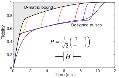
Figure 3: The black solid line bounds the maximum fidelity of a single-qubit Hadamard gate implemented in a two-level system with $H=\hbar\omega_{0}\sigma_{z}-\mu\varepsilon(t)\sigma_{x}$, and maximum control amplitude $\varepsilon_{\rm max}=1$. Pulses optimized for different final times (colored lines) can achieve the upper bounds at all times.

Conclusions—Quadratic constraints representing generalized probability-conservation laws offer a framework for quantum control bounds. We have shown that this method can be significantly tighter than previous bounds and more widely applicable. There are further extensions that may be possible as well: in nanophotonic design problems, a hierarchy of bounds with varying analytical and semi-analytical complexity have been discovered as subsets of the $D$-matrix constraints [74, 75, 76, 77, 78, 79, 80, 81, 82, 83, 84, 1, 2, 61]; the same may be possible in quantum control. In particular, environment-induced decoherence and dissipation are similar to material-absorption losses in electromagnetism, and may be amenable to general analytical bounds [74, 78]. From an algorithmic perspective, there are significant computational speed-ups that should make the bound computations competitive with local optimizations, as a function of the number of degrees of freedom of the system, $N$ (the product of time steps and Hilbert-space dimensionality). Global optimization is presumably NP-hard; local optimizations require $O(N)$ time for each iteration and a number of iterations that may be large but independent of $N$. To find good local optima, however, requires restarting the search a number of times proportional to the number of local optima, which should scale at least as $O(N)$, for a total scaling of at least $O(N^{2})$ (which is likely optimistic). For the bound computations, the simple implementation used for this work, using all possible constraints and interior-point-methods oblivious to the structure of the problem, scales as $O(N^{4.5})$ [85]. Clever selection of the constraint matrices [1] can reduce the scaling to $O(N^{3.5})$, while exploitation of the integral-operator’s structure (e.g. via fast-multipole-type methods [86, 87]) should further improve the scaling to $O(N^{2.5})$, making it highly competitive with local design methods. More broadly, our approach and extensions thereof can be applied to problems across the quantum-control landscape, ranging from speed limits and gate fidelity to areas like NMR [6, 7, 8] and quantum complexity [9, 10, 11].

References

- Kuang and Miller [2020] Z. Kuang and O. D. Miller, Computational bounds to light–matter interactions via local conservation laws, Phys. Rev. Lett. 125, 263607 (2020), arXiv:2008.13325 .
- Molesky et al. [2020a] S. Molesky, P. Chao, and A. W. Rodriguez, Hierarchical mean-field T operator bounds on electromagnetic scattering: Upper nounds on near-field radiative Purcell enhancement, Phys. Rev. Res. 2, 043398 (2020a), arXiv:2008.08168 .
- Laurent and Rendl [2005] M. Laurent and F. Rendl, Semidefinite Programming and Integer Programming, Handbooks Oper. Res. Manag. Sci. 12, 393 (2005).
- Luo et al. [2010] Z. Q. Luo, W. K. Ma, A. So, Y. Ye, and S. Zhang, Semidefinite relaxation of quadratic optimization problems, IEEE Signal Process. Mag. 27, 20 (2010).
- Motzoi et al. [2009] F. Motzoi, J. M. Gambetta, P. Rebentrost, and F. K. Wilhelm, Simple pulses for elimination of leakage in weakly nonlinear qubits, Physical Review Letters 103, 110501 (2009).
- Khaneja et al. [2005] N. Khaneja, T. Reiss, C. Kehlet, T. Schulte-Herbrüggen, and S. J. Glaser, Optimal control of coupled spin dynamics: Design of NMR pulse sequences by gradient ascent algorithms, J. Magn. Reson. 172, 296 (2005).
- Nielsen et al. [2010] N. C. Nielsen, C. Kehlet, S. J. Glaser, and N. Khaneja, Optimal Control Methods in NMR Spectroscopy, Encycl. Magn. Reson. 10.1002/9780470034590.emrstm1043 (2010).
- Tošner et al. [2018] Z. Tošner, R. Sarkar, J. Becker-Baldus, C. Glaubitz, S. Wegner, F. Engelke, S. J. Glaser, and B. Reif, Overcoming Volume Selectivity of Dipolar Recoupling in Biological Solid-State NMR Spectroscopy, Angew. Chemie Int. Ed. 57, 14514 (2018).
- Nielsen et al. [2006] M. A. Nielsen, M. R. Dowling, M. Gu, and A. C. Doherty, Optimal control, geometry, and quantum computing, Phys. Rev. A 73, 1 (2006), arXiv:0603160 [quant-ph] .
- Jefferson and Myers [2017] R. A. Jefferson and R. C. Myers, Circuit complexity in quantum field theory, J. High Energy Physics 2017, 107 (2017).
- Chapman et al. [2018] S. Chapman, M. P. Heller, H. Marrochio, and F. Pastawski, Toward a Definition of Complexity for Quantum Field Theory States, Phys. Rev. Lett. 120, 121602 (2018).
- Peirce et al. [1988] A. P. Peirce, M. A. Dahleh, and H. Rabitz, Optimal control of quantum-mechanical systems: Existence, numerical approximation, and applications, Phys. Rev. A 37, 4950 (1988).
- Werschnik and Gross [2007] J. Werschnik and E. K. Gross, Quantum optimal control theory, J. Phys. B At. Mol. Opt. Phys. 40, 10.1088/0953-4075/40/18/R01 (2007), arXiv:0707.1883 .
- D’Alessandro [2007] D. D’Alessandro, Introduction to quantum control and dynamics (CRC press, Boca Raton, FL, 2007).
- Brif et al. [2010] C. Brif, R. Chakrabarti, and H. Rabitz, Control of quantum phenomena: Past, present and future, New J. Phys. 12, 10.1088/1367-2630/12/7/075008 (2010), arXiv:0912.5121 .
- Glaser et al. [2015] S. J. Glaser, U. Boscain, T. Calarco, C. P. Koch, W. Köckenberger, R. Kosloff, I. Kuprov, B. Luy, S. Schirmer, T. Schulte-Herbrüggen, D. Sugny, and F. K. Wilhelm, Training Schrödinger’s cat: Quantum optimal control: Strategic report on current status, visions and goals for research in Europe, Eur. Phys. J. D 69, 10.1140/epjd/e2015-60464-1 (2015).
- Bason et al. [2012] M. G. Bason, M. Viteau, N. Malossi, P. Huillery, E. Arimondo, D. Ciampini, R. Fazio, V. Giovannetti, R. Mannella, and O. Morsch, High-fidelity quantum driving, Nat. Phys. 8, 147 (2012), arXiv:1111.1579 .
- Van Frank et al. [2016] S. Van Frank, M. Bonneau, J. Schmiedmayer, S. Hild, C. Gross, M. Cheneau, I. Bloch, T. Pichler, A. Negretti, T. Calarco, and S. Montangero, Optimal control of complex atomic quantum systems, Sci. Rep. 6, 34187 (2016), arXiv:1511.02247 .
- Heeres et al. [2017] R. W. Heeres, P. Reinhold, N. Ofek, L. Frunzio, L. Jiang, M. H. Devoret, and R. J. Schoelkopf, Implementing a universal gate set on a logical qubit encoded in an oscillator, Nat. Commun. 8, 1 (2017), arXiv:1608.02430 .
- Goetz et al. [2019] R. E. Goetz, C. P. Koch, and L. Greenman, Quantum Control of Photoelectron Circular Dichroism, Phys. Rev. Lett. 122, 13204 (2019), arXiv:1809.04543 .
- Vepsäläinen et al. [2019] A. Vepsäläinen, S. Danilin, and G. S. Paraoanu, Superadiabatic population transfer in a three-level superconducting circuit, Sci. Adv. 5, eaau5999 (2019).
- Lam et al. [2021] M. R. Lam, N. Peter, T. Groh, W. Alt, C. Robens, D. Meschede, A. Negretti, S. Montangero, T. Calarco, and A. Alberti, Demonstration of Quantum Brachistochrones between Distant States of an Atom, Phys. Rev. X 11, 11035 (2021), arXiv:2009.02231 .
- De Fouquieres et al. [2011] P. De Fouquieres, S. G. Schirmer, S. J. Glaser, and I. Kuprov, Second order gradient ascent pulse engineering, J. Magn. Reson. 212, 412 (2011).
- Dolde et al. [2014] F. Dolde, V. Bergholm, Y. Wang, I. Jakobi, B. Naydenov, S. Pezzagna, J. Meijer, F. Jelezko, P. Neumann, T. Schulte-Herbrüggen, J. Biamonte, and J. Wrachtrup, High-fidelity spin entanglement using optimal control, Nat. Commun. 5, 1 (2014), arXiv:1309.4430 .
- Anderson et al. [2015] B. E. Anderson, H. Sosa-Martinez, C. A. Riofrío, I. H. Deutsch, and P. S. Jessen, Accurate and Robust Unitary Transformations of a High-Dimensional Quantum System, Phys. Rev. Lett. 114, 240401 (2015).
- Krotov [1993] V. F. Krotov, Global Methods in Optimal Control Theory, in Adv. Nonlinear Dyn. Control A Rep. from Russ. (Birkhäuser Boston, 1993) pp. 74–121.
- Somlói et al. [1993] J. Somlói, V. A. Kazakov, and D. J. Tannor, Controlled dissociation of I2 via optical transitions between the X and B electronic states, Chem. Phys. 172, 85 (1993).
- Zhu and Rabitz [1998] W. Zhu and H. Rabitz, A rapid monotonically convergent iteration algorithm for quantum optimal control over the expectation value of a positive definite operator, J. Chem. Phys. 109, 385 (1998).
- Ohtsuki et al. [2004] Y. Ohtsuki, G. Turinici, and H. Rabitz, Generalized monotonically convergent algorithms for solving quantum optimal control problems, J. Chem. Phys. 120, 5509 (2004).
- Schirmer and De Fouquieres [2011] S. G. Schirmer and P. De Fouquieres, Efficient algorithms for optimal control of quantum dynamics: The Krotov method unencumbered, New J. Phys. 13, 73029 (2011), arXiv:1103.5435 .
- Goerz et al. [2019] M. H. Goerz, D. Basilewitsch, F. Gago-Encinas, M. G. Krauss, K. P. Horn, D. M. Reich, and C. P. Koch, Krotov: A Python implementation of Krotov’s method for quantum optimal control, SciPost Phys. 7, 080 (2019), arXiv:1902.11284 .
- Caneva et al. [2011] T. Caneva, T. Calarco, and S. Montangero, Chopped random-basis quantum optimization, Phys. Rev. A 84, 022326 (2011).
- Doria et al. [2011] P. Doria, T. Calarco, and S. Montangero, Optimal control technique for many-body quantum dynamics, Phys. Rev. Lett. 106, 1 (2011).
- Mandelstam and Tamm [1945] L. Mandelstam and I. Tamm, The Uncertainty Relation Between Energy and Time in Non-relativistic Quantum Mechanics, J. Phys. USSR 9, 249 (1945).
- Fleming [1973] G. N. Fleming, A unitarity bound on the evolution of nonstationary states, Nuovo Cim. A 16, 232 (1973).
- Vaidman [1992] L. Vaidman, Minimum time for the evolution to an orthogonal quantum state, Am. J. Phys. 60, 182 (1992).
- Margolus and Levitin [1998] N. Margolus and L. B. Levitin, The maximum speed of dynamical evolution, Phys. D Nonlinear Phenom. 120, 188 (1998), arXiv:9710043 [quant-ph] .
- Khaneja et al. [2001] N. Khaneja, R. Brockett, and S. J. Glaser, Time optimal control in spin systems, Phys. Rev. A - At. Mol. Opt. Phys. 63, 032308 (2001), arXiv:0006114 [quant-ph] .
- Khaneja et al. [2002] N. Khaneja, S. J. Glaser, and R. Brockett, Sub-Riemannian geometry and time optimal control of three spin systems: Quantum gates and coherence transfer, Phys. Rev. A 65, 032301 (2002), arXiv:0106099 [quant-ph] .
- Giovannetti et al. [2003a] V. Giovannetti, S. Lloyd, and L. Maccone, Quantum limits to dynamical evolution, Phys. Rev. A - At. Mol. Opt. Phys. 67, 8 (2003a), arXiv:0210197 [quant-ph] .
- Giovannetti et al. [2003b] V. Giovannetti, S. Lloyd, and L. Maccone, The role of entanglement in dynamical evolution, Europhys. Lett. 62, 615 (2003b).
- Carlini et al. [2006] A. Carlini, A. Hosoya, T. Koike, and Y. Okudaira, Time-optimal quantum evolution, Phys. Rev. Lett. 96, 1 (2006).
- Carlini et al. [2007] A. Carlini, A. Hosoya, T. Koike, and Y. Okudaira, Time-optimal unitary operations, Phys. Rev. A - At. Mol. Opt. Phys. 75, 1 (2007), arXiv:0608039 [quant-ph] .
- Deffner and Lutz [2013] S. Deffner and E. Lutz, Quantum speed limit for non-Markovian dynamics, Phys. Rev. Lett. 111, 1 (2013), arXiv:1302.5069 .
- Del Campo et al. [2013] A. Del Campo, I. L. Egusquiza, M. B. Plenio, and S. F. Huelga, Quantum speed limits in open system dynamics, Phys. Rev. Lett. 110, 10.1103/PhysRevLett.110.050403 (2013), arXiv:1209.1737 .
- Poggi et al. [2013] P. M. Poggi, F. C. Lombardo, and D. A. Wisniacki, Quantum speed limit and optimal evolution time in a two-level system, EPL (Europhysics Lett. 104, 40005 (2013).
- Hegerfeldt [2013] G. C. Hegerfeldt, Driving at the quantum speed limit: Optimal control of a two-level system, Phys. Rev. Lett. 111, 1 (2013), arXiv:1305.6403 .
- Hegerfeldt [2014] G. C. Hegerfeldt, High-speed driving of a two-level system, Phys. Rev. A - At. Mol. Opt. Phys. 90, 1 (2014), arXiv:1407.6502 .
- Russell and Stepney [2014] B. Russell and S. Stepney, Zermelo navigation and a speed limit to quantum information processing, Phys. Rev. A - At. Mol. Opt. Phys. 90, 1 (2014), arXiv:1310.6731 .
- Brody and Meier [2015] D. C. Brody and D. M. Meier, Solution to the quantum Zermelo navigation problem, Phys. Rev. Lett. 114, 1 (2015), arXiv:1409.3204 .
- Russell and Stepney [2015] B. Russell and S. Stepney, Zermelo navigation in the quantum brachistochrone, J. Phys. A Math. Theor. 48, 115303 (2015).
- Frey [2016] M. R. Frey, Quantum speed limits—primer, perspectives, and potential future directions, Quantum Inf. Process. 15, 3919 (2016).
- Deffner and Campbell [2017] S. Deffner and S. Campbell, Quantum speed limits: From Heisenberg’s uncertainty principle to optimal quantum control, J. Phys. A Math. Theor. 50, 453001 (2017).
- Arenz et al. [2017] C. Arenz, B. Russell, D. Burgarth, and H. Rabitz, The roles of drift and control field constraints upon quantum control speed limits, New J. Phys. 19, 103015 (2017).
- Lee et al. [2018] J. Lee, C. Arenz, H. Rabitz, and B. Russell, Dependence of the quantum speed limit on system size and control complexity, New J. Phys. 20, 063002 (2018).
- Burgarth et al. [2020] D. Burgarth, J. Borggaard, and Z. Zimborás, Quantum distance to uncontrollability and quantum speed limits, arXiv preprint arXiv:2010.16156 (2020).
- Knowles [1981] G. Knowles, An Introduction to Applied Optimal Control (Academic Press, Inc., New York, NY, 1981).
- Englert [2006] B.-G. Englert, Lectures On Quantum Mechanics-Volume 3: Perturbed Evolution (World Scientific Publishing Company, 2006).
- Sakurai [1994] J. J. Sakurai, Modern Quantum Mechanics, edited by S. F. Tuan (Addison-Wesley Publishing Co., Reading, MA, 1994).
- Jackson [1999] J. D. Jackson, Classical Electrodynamics, 3rd Ed. (John Wiley & Sons, 1999).
- Angeris et al. [2021] G. Angeris, J. Vučković, and S. Boyd, Heuristic methods and performance bounds for photonic design, Opt. Express 29, 2827 (2021), arXiv:2011.08002 .
- Thijssen [2012] J. Thijssen, Computational Physics (Cambridge University Press, 2012).
- Vandenberghe and Boyd [1996] L. Vandenberghe and S. Boyd, Semidefinite Programming, SIAM Rev. 38, 49 (1996).
- Krantz et al. [2019] P. Krantz, M. Kjaergaard, F. Yan, T. P. Orlando, S. Gustavsson, and W. D. Oliver, A quantum engineer’s guide to superconducting qubits, Applied Physics Reviews 6, 021318 (2019).
- Wood and Gambetta [2018] C. J. Wood and J. M. Gambetta, Quantification and characterization of leakage errors, Phys. Rev. A 97, 032306 (2018), arXiv:1704.03081 .
- Viola et al. [1999] L. Viola, E. Knill, and S. Lloyd, Dynamical decoupling of open quantum systems, Physical Review Letters 82, 2417 (1999).
- Uhrig [2009] G. S. Uhrig, Concatenated control sequences based on optimized dynamic decoupling, Physical Review Letters 102, 120502 (2009).
- West et al. [2010] J. R. West, D. A. Lidar, B. H. Fong, and M. F. Gyure, High fidelity quantum gates via dynamical decoupling, Physical Review Letters 105, 230503 (2010).
- Souza et al. [2011] A. M. Souza, G. A. Alvarez, and D. Suter, Robust dynamical decoupling for quantum computing and quantum memory, Physical Review Letters 106, 240501 (2011).
- Rossini et al. [2008] D. Rossini, P. Facchi, R. Fazio, G. Florio, D. A. Lidar, S. Pascazio, F. Plastina, and P. Zanardi, Bang-bang control of a qubit coupled to a quantum critical spin bath, Physical Review A 77, 052112 (2008).
- Kosloff [2019] R. Kosloff, Quantum thermodynamics and open-systems modeling, The Journal of Chemical Physics 150, 204105 (2019).
- Khodjasteh and Lidar [2005] K. Khodjasteh and D. A. Lidar, Fault-tolerant quantum dynamical decoupling, Physical Review Letters 95, 180501 (2005).
- Viola and Knill [2003] L. Viola and E. Knill, Robust dynamical decoupling of quantum systems with bounded controls, Physical Review Letters 90, 037901 (2003).
- Miller et al. [2016] O. D. Miller, A. G. Polimeridis, M. T. H. Reid, C. W. Hsu, B. G. Delacy, J. D. Joannopoulos, M. Soljačic̀, and S. G. Johnson, Fundamental limits to optical response in absorptive systems, Optics Express 24, 3329 (2016).
- Yang et al. [2017] Y. Yang, O. D. Miller, T. Christensen, J. D. Joannopoulos, and M. Soljačic̀, Low-loss plasmonic dielectric nanoresonators, Nano Letters 17, 3238 (2017).
- Shim et al. [2019] H. Shim, L. Fan, S. G. Johnson, and O. D. Miller, Fundamental Limits to Near-Field Optical Response over Any Bandwidth, Phys. Rev. X 9, 11043 (2019).
- Molesky et al. [2019] S. Molesky, W. Jin, P. S. Venkataram, and A. W. Rodriguez, T Operator Bounds on Angle-Integrated Absorption and Thermal Radiation for Arbitrary Objects, Phys. Rev. Lett. 123, 257401 (2019).
- Ivanenko et al. [2019] Y. Ivanenko, M. Gustafsson, and S. Nordebo, Optical theorems and physical bounds on absorption in lossy media, Opt. Express 27, 34323 (2019), arXiv:1908.09657 .
- Shim et al. [2020a] H. Shim, H. Chung, and O. D. Miller, Maximal free-space concentration of electromagnetic waves, Physical Review Applied 14, 014007 (2020a), 1905.10500 .
- Shim et al. [2020b] H. Shim, Z. Kuang, and O. D. Miller, Optical materials for maximal nanophotonic response (Invited), Optical Materials Express 10, 1561 (2020b), arXiv:2004.13132 .
- Molesky et al. [2020b] S. Molesky, P. Chao, W. Jin, and A. W. Rodriguez, Global T operator bounds on electromagnetic scattering: Upper bounds on far-field cross sections, Phys. Rev. Res. 2, 033172 (2020b).
- Gustafsson et al. [2020] M. Gustafsson, K. Schab, L. Jelinek, and M. Capek, Upper bounds on absorption and scattering, New J. Phys. 22, 073013 (2020), arXiv:1912.06699 .
- Molesky et al. [2020c] S. Molesky, P. S. Venkataram, W. Jin, and A. W. Rodriguez, Fundamental limits to radiative heat transfer: Theory, Phys. Rev. B 101, 35408 (2020c), arXiv:1907.03000 .
- Kuang et al. [2020] Z. Kuang, L. Zhang, and O. D. Miller, Maximal single-frequency electromagnetic response, Optica 7, 1746 (2020), arXiv:2002.00521 .
- Ma et al. [2008] W.-K. Ma, C.-C. Su, J. Jaldén, and C.-Y. Chi, Some results on 16-qam mimo detection using semidefinite relaxation, in 2008 IEEE International Conference on Acoustics, Speech and Signal Processing (IEEE, 2008) pp. 2673–2676.
- Greengard and Rokhlin [1987] L. Greengard and V. Rokhlin, A fast algorithm for particle simulations, Journal of Computational Physics 73, 325 (1987).
- Coifman et al. [1993] R. Coifman, V. Rokhlin, and S. Wandzura, The fast multipole method for the wave equation: A pedestrian prescription, IEEE Antennas and Propagation magazine 35, 7 (1993).