GPSglobal positioning system[GPS] FFTfast Fourier transform[FFT] BGIBureau Gravim$\acute{\rm e}$trique International[BGI98] NKGNordic Geodetic Commission[NKG] OCTASOcean Circulation and Transport Between North Atlantic and the Arctic Sea[OCTAS] GOCINAGeoid and Ocean Circulation in the North Atlantic[GOCINA] OCCAMOcean Circulation and Climate Advanced Modelling[OCCAM] NIMANational Imagery and Mapping Agency[NIMA] NMCANorwegian Mapping and Cadastre Authority[NMCA] NMANorwegian Mapping Authority[NMA] IGNInstitut Geographique National[IGN] IGSInternational GNSS Service[IGS] IVSInternational VLBI Service[IVS] IDSInternational DORIS Service[IDS] ITRSInternational Terrestrial Reference System[ITRF] ITRFInternational Terrestrial Reference Frame[ITRF2014] IERSInternational Earth Rotation Service[IERS] GNSSGlobal Navigation Satellite System[GNSS] VLBIVery Long Baseline Interfer[VLBI] CGPSContinuous GPS[CGPS] DGPSDifferential GPS[DGPS] DoDDepartment of Defence[DoD] DORISDoppler Orbitography and Radiopositioning Integrated by Satellites[DORIS] EGMEarth Gravity Model[EGM] EGNOSEuropean Geostationary Navigation Overlay Service[EGNOS] EOPEarth Orientation Parameters[EOP] ESAEuropean Space Agency[ESA] ESOCEuropean Space Operation Centre[ESOC] ESEASEuropean Sea Level Service[ESEAS] ESEAS-RIESEAS Research Infrastructure[ESEAS-RI] ETRSEuropean Terrestrial Reference System[ETRS] EUREFIAG Reference Frame Sub-Commission for Europe[EUREF] EPNEUREF Permanent Network[EPN] NGSNational Geodetic Survey[NGS] GAMITGPS Analysis Software of MIT[GAMIT] GIPSYGNSS-Inferred Positioning System[GIPSY] GLONASSGlobal Navigation Satellite System[GLONAS] GPSGlobal Positioning System[GPS] IERSInternational Earth Rotation Service[IERS] IGS-TIGAIGS-Tide Gauge Benchmark Monitoring [IGS-TIGA] JPLJet Propulsion Laboratory[JPL] UNRUniversity of Nevada, Reno[UNR] MITMassachusetts Institute of Technology[MIT] NIMANational Imagery and Mapping Agency[NIMA] NNSSNavy Navigation satellite system[NNSS] NLESNavigation Land Earth Station[NLES] NASANational Aeronautics & Space Administration[NASA] OSOOnsala Space Observatory[OSO] RIMSRanging and Integrity Monitoring Station[RIMS] RINEXReceiver independent exchange format[RINEX] SINEXSite independent exchange format[SINEX] SLRSatellite Laser Ranging[SLR] SOPACScripps Orbits and Permanent Array Center[SOPAC] SWEPOSSwedish GPS Network[SWEPOS] SATREFSatellite based reference system[SATREF] VLBIVery Long Baseline Interferometry[VLBI] WGS84World Geodetic System 1984[WGS84] GFZGeoForschungsZentrum Potsdam[GFZ] GIGGPS IERS and Geodynamics 1991[GIG91] PPPPrecise Point Positioning[PPP] CHAMPCHAllenging Minisatellite Payload[CHAMP] ASAntispoofing[AS] GRACEGravity Recovery and Climate Experiment[GRACE] PGRPost Glacial Rebound[PGR] PDIMPresent Day Ice Melt[PDIM] TGBTide Gauge Benchmar[TGB] SCGSuper Conducting Gravity[SCG] GGOSGlobal Geodetic Observing System[GGOS] DDDouble Difference[DD] IPEVFrench Polar Institute - Paul Emile Victor[IPEV] LSQLeast Square[LS] PSMSLPermanent Service for Mean Sea Level[PSMSL] PCVPhase Center Variation[PCV] GIAGlacial Isostatic Adjustment[GIA] GLOBKGlobal Kalman filter VLBI and GPS analysis program[GLOBK] BIFROSTBaseline Inferences for Fennoscandian Rebound, Sea-level, and Tectonics[BIFROST] QIFQuasi Ionosphere Free[QIF] VMFVienna Mapping Functions[VMF1] LGMLatest Glacial Maximum[LGM] SRIFSquare root information filter[SRIF] CORSContinuously Operating Reference Station[CORS] epGNSSepisodic GNSS stations[epGNSS] cGNSScontinuous operating GNSS stations[cGNSS] RTKReal Time Kinematic[RTK] VGOSVLBI Global Observing System[VGOS] CMSCommon Mode Signal[CMS] CMCommon Mode[CM] LCMLoad and Common Mode[LCM] EOFEmpirical Ortoghonal Functions[EOF] LIALittle Ice Age[LIA] CMBClimatic Mass Balance[CMB] GSGlaciers and Snow[GS] ATMAtmospheric[ATM] NTONon-Tidal Ocean[NTO] HYDHydrological[HYD] AOH[] RMSRoot Mean Square[RMS] LWSLand Water Storage[LWS] NTLNon-tidal loading[NTL] NNRNo-Net-Rotation[NNR]

Seasonal glacier and snow loading in Svalbard recovered from geodetic observations

We processed time series from seven Global Navigation Satellite System (GNSS) stations and one Very Long Baseline Interferometry (VLBI) station in Svalbard. The goal was to capture the seasonal vertical displacements caused by elastic response of variable mass load due to ice and snow accumulation. We found that estimates of the annual signal in different GNSS solutions disagree by more than 3 mm which makes geophysical interpretation of raw GNSS time series problematic. To overcome this problem, we have used an enhanced Common Mode (CM) filtering technique. The time series are differentiated by the time series from remote station BJOS with known mass loading signals removed a priori. Using this technique, we have achieved a substantial reduction of the differences between the GNSS solutions. We have computed mass loading time series from a regional Climatic Mass Balance (CMB) and snow model that provides the amount of water equivalent at a 1 km resolution with a time step of 7 days. We found that the entire vertical loading signal is present in data of two totally independent techniques at a statistically significant level of 95%. This allowed us to conclude that the remaining errors in vertical signal derived from the CMB model are less than 0.2 mm at that significance level. Refining the land water storage loading model with a CMB model resulted in a reduction of the annual amplitude from $2.1$ mm to $1.1$ mm in the CM filtered time series, while it had only a marginal impact on raw time series. This provides a strong evidence that CM filtering is essential for revealing local periodic signals when a millimetre level of accuracy is required.

1 Introduction

The Arctic archipelago Svalbard is exposed to climate change phenomena, the temperature is rising, the permafrost is melting, the sea level is rising, and the glaciers are retreating (Hanssen-Bauer et al., 2019). Consequences of climate change, like sea-level rise or increased land-uplift, can be observed by geodetic techniques in an accurate geodetic reference frame. On the other hand, these changes challenge the stability of the geodetic reference frame itself, e.g., the increased land uplift will deform the reference frame over time. Knowledge about the interaction between geophysical processes, crustal deformations and reference frame is mandatory to achieve the GGOS2020 goal of a reference frame with a stability of $0.1$ mm/yr (Plag & Pearlman, 2009).

The geodetic observatory in Ny-Ålesund is one of the core stations in the global geodetic network. It was established during the 1990s with  antennas,  telescope, , absolute gravity points, and control networks (Kierulf et al., 2009a).

Due to Svalbard’s remote location and challenging environmental conditions Ny-Ålesund was for a long time the only location with permanent geodetic equipment on the archipelago. Sato et al. (2006b, a) studied the gravity signal in Ny-Ålesund and the interaction between gravity changes and uplift. The uplift in Ny-Ålesund is not linear. It has a seasonal component, that will be studied in details in this manuscript, and an inter-annual signal induced by the long term (years to decades) evolution of glacier mass balance (e.g. Kierulf et al., 2009a). Kierulf et al. (2009b) showed that the uplift changed from year to year and that these variations are very well explained by the changes in the mass balance of the nearby glaciers. Omang & Kierulf (2011) found that also the gravity rate is changing with time. Mémin et al. (2012) showed that topography of glaciers has a significant effect on the gravity rate. The visco-elastic response of the last ice age (Auriac et al., 2016) and the visco-elastic response of the glacier retreat after the  (Mémin et al., 2014) also contribute to the uplift in Ny-Ålesund. In 2005, the Polish research station in Hornsund installed a new GNSS antenna. Rajner (2018) compared results from the stations in Hornsund and Ny-Ålesund and demonstrated that both locations have non-linear uplift. All these papers focus mainly on glacier related phenomena with time spans ranging from years to decades or thousands of years.

The most prominent variations in snowpack and glacier mass are the annual cycle with accumulation of snow each winter and melting in the short Arctic summer. The crusts elastic response of this seasonal variations results in a seasonal cycle also in the GNSS station coordinates and other geodetic equipment. The crust is also exposed to  from atmosphere, ocean and land water (Petrov & Boy, 2004; Mémin et al., 2020).

The main questions in this paper are: (1) How well do GNSS and VLBI capture the seasonal signal from glaciers and snow in Svalbard? (2) Will refining the  models with a  model improve the loading predictions? To answer these two questions we have studied GNSS time series from six locations on Svalbard (see Fig. 1) and the VLBI antenna in Ny-Ålesund. We have used different analysis strategies both for the GNSS and the VLBI data sets. We have also filtered our time series for  and  signals to improve the regional accuracy. The model described in van Pelt et al. (2019) simulates glacier  and seasonal snow conditions, from which variations in loading from glaciers and snowpack are extracted.

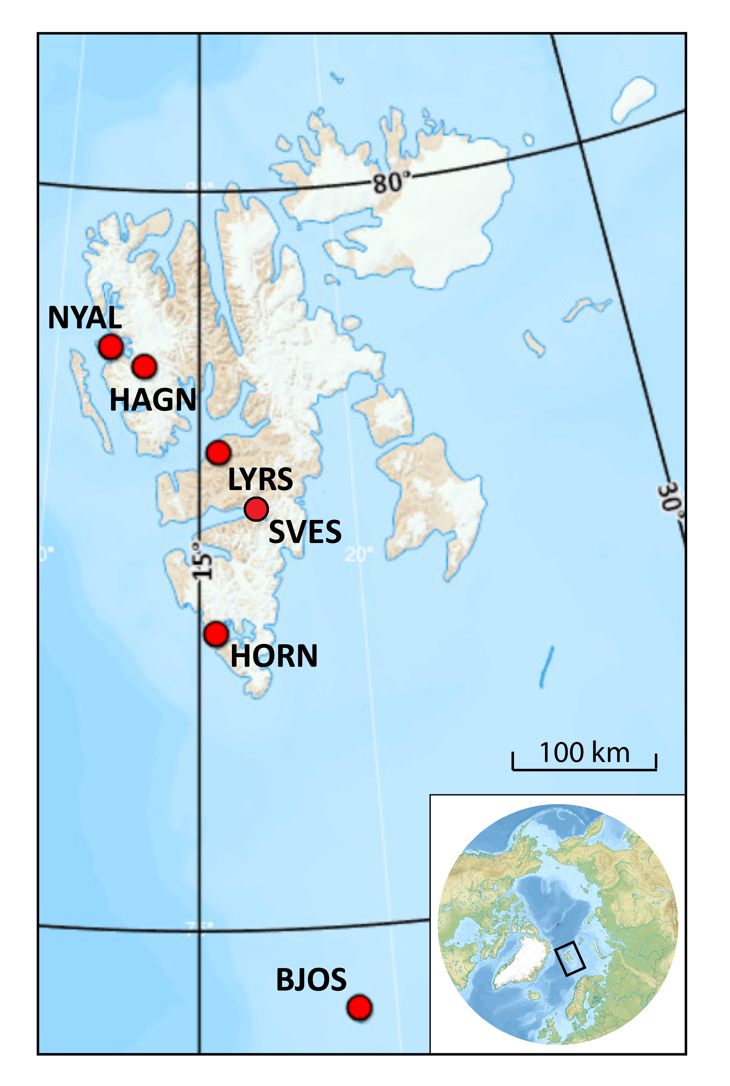
Figure 1: Geodetic network on Svalbard. The location NYAL include the GNSS stations NYAL and NYA1, the VLBI antenna NYALES20 and the SCG instrument.

In Section 2 we describe the different data sets used in this study. We describe the softwares and analysis strategies for geodetic analysis, the time series analysis, the  filtering and the different models used for loading predictions. In Section 3, we compare the geodetic results with the loading signal from glaciers and snow, ,  and . Based on this we discuss possibilities and limitations in our solutions for revealing the seasonal elastic signal. We also study the effect of refining the hydrological model with the  model (Subsection 3.4).

2 Data and data analysis

2.1 CMB model

Glacier mass change is primarily the result of surface - atmosphere interactions (affecting snow accumulation and melt), snow processes (affecting melt water retention and runoff) and frontal processes (calving and frontal ablation of tidewater glaciers). Glacier mass changes due to atmosphere - surface - snow interactions are described by the , which describes the mass change of a vertical column of snow/firn/ice, in response to surface mass, and energy exchange and runoff of melt water. The  dominates seasonal glacier mass change, with mass gain from snow accumulation during the cold season and melt-driven mass loss during the melt season.

Noël et al. (2020) have shown that for all glaciers in Svalbard the mass fluxes of precipitation (+23 Gt/yr) and runoff (-25 Gt/yr) dominate the seasonal climatic mass balance cycle in recent decades (1985-2018), with nearly all runoff concentrated in the summer months (June, July and August) and snow accumulating the rest of the year. These mass fluxes are much larger than the estimated mean ice discharge due to calving and frontal ablation from tidewater glaciers (7 Gt/yr Błaszczyk et al., 2009). Svalbard-wide constraints on the seasonality of combined calving and frontal ablation are currently lacking and not considered here. Previous estimates on three glaciers in Svalbard however indicate that frontal ablation is more substantial in summer and early autumn than during winter and spring (Luckman et al., 2015).

Here, we use the  model data set, described in van Pelt et al. (2019), and extract weekly output for the period 1990-2018. van Pelt et al. (2019) used a coupled energy balance - subsurface model (van Pelt et al., 2012) to simulate  for all glaciers in Svalbard, as well as seasonal snow conditions in non-glacier terrain. Both the glacier and seasonal snow mass changes are accounted for. They describe weekly mass changes resulting from snow accumulation, surface moisture exchange, melt and rain water refreezing, and retention in snow, and runoff. Runoff estimates are local and no horizontal transport of water is accounted for.

2.2 Elastic loading signal

Mass redistribution results in Earth’s crust deformation called mass loading (Darwin, 1882). Mass loadings are caused by the ocean water mass redistribution due to gravitational tides and pole tide (ocean tidal loading), by variations of the atmospheric mass ( loading), by variations of the bottom ocean pressure due to ocean circulation ( loading), and by variations of land water mass stored in soil, snow, and ice ( loading). Mass loading crustal deformations have a typical magnitude at a centimetre level (see e.g. Petrov & Boy, 2004).

Love (1911) showed that the deformation caused by mass loadings can be found in a form of an expansion into spherical harmonics. Each spherical harmonic of the deformation field is proportional to the spherical harmonic of the surface pressure exerted by loading mass. The proportionality dimensionless coefficients called Love numbers that depend on a harmonic degree are found by solving differential equations. Therefore, when the global pressure field mass redistribution is known, the elastic deformation can be found by expansion of that field into spherical harmonics, scaling the harmonics by Love numbers and performing an inverse spherical harmonics expansion.

Love numbers were computed using the REAR software (Melini et al., 2015) for the Earth reference model STW105 (Kustowski et al., 2008). Time series of  from ,  and  have been used in our analysis. Input to the  loading is the pressure field from NASA’s numerical weather model MERRA2 (Gelaro et al., 2017). The  loading uses the model MPIOM06 (Jungclaus et al., 2013), and the  loading uses the pressure field of MERRA2 model (Reichle et al., 2011). The MERRA2 model accounts for soil moisture at the depth of 0–2 meter and accumulated snow. 3D displacements cause by these loadings were computed using spherical harmonics transform of degree and order 2699 and presented at a global grid $2^{\prime}\times 2^{\prime}$ with a time step of 3 or 6 hours. Then mass loading at a given station is found by interpolation. The time series of these loadings are available at the International Mass Loading Service http://massloading.net (Petrov, 2017).

However, the MERRA2 numerical weather model do not adequately describe accumulation and runoff of water, snow, and ice at glaciers. It does not consider all complexity of glacial mass change processes and its resolution, 16x55 km, is insufficient to catch fine details in Svalbard. Here, we test the impact of replacing the above global model component for snow and ice with the regional snow and glacier  product with $1\times 1$ km resolution. The model is described in Section 2.1. We have re-gridded the $1\times 1$ km model to a uniform, regular, latitude-longitude grid with a resolution of $30^{\prime\prime}\times 30^{\prime\prime}$. The model value at a given element of the new grid is

$$M_{ij}=\frac{\displaystyle\sum_{ab}M_{ab}e^{-r_{ij,ab}/D}}{\displaystyle\sum_{ab}e^{-r_{ij,ab}/D}},$$ (1)

where $M_{ab}$ is the model value for element a,b, the $r_{ij,ab}$ is the distance between grid points i,j and a,b, and $D$ is the kernel distance set to 1 km.

We have computed mass loading time series, from 1990-08-05 through 2018-08-26 with a step of 7 days, at a $30^{\prime\prime}\times 30^{\prime\prime}$ grid from the  output using spherical harmonic expansion degree and order 10799. This high resolution was used to correctly model the signal at stations that are located close to the edge of glaciers.

The choice of the degree/order of the expansion is determined by availability of computing resources. The higher degree/order of the spherical harmonic transform, the less errors near the coastal line. Atmospheric, land-water storage, and non-tidal ocean loading are computed with the time resolution of 3 hours and the total computation time using degree/order 2699 is about 4 years per single core for CPUs produced in 2015–2020. Since the glacier model has time resolution of 7 days we can afford to run computation with degree/order 10799 which allows to correctly model the signal at stations that are located close to the edge of glaciers.

However, it is not sufficient to replace the  loading computed on the basis of MERRA2 model with the mass loading computed on the basis of the  model. Crustal deformation at a given point is affected by mass loading not only from the close vicinity, but also from remote areas. Therefore, in order to account for loading displacement caused by mass redistribution from the area beyond Svalbard archipelago, we computed an additional series of  loading using MERRA2 model that was set to zero outside Svalbard archipelago. The total  loading displacement is:

$$D_{\rm LWS}=D_{\rm merra2}-D_{\rm merra2,svalbrard}+D_{CMB},$$ (2)

where $D_{\rm merra2}$ is the displacement from MERRA2 model, $D_{\rm merra2,svalbrard}$ is the loading signal from the MERRA2 model that was set to zero except latitude $76^{\circ}<\phi<81^{\circ}$ and longitude $10^{\circ}<\lambda<34^{\circ}$ (the area including the Svalbard archipelago) and $D_{CMB}$ is the displacement form the  model.

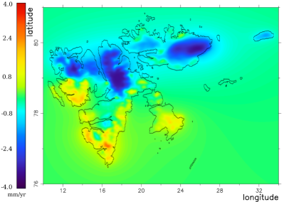
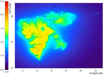
Figure 2: Crustal deformations due to glacier and snow loading according to the CMB model. The panels are: the rate of change (left) and annual signal (right). Important: the CMB model does not account for mass loss due to frontal ablation and calving.

Fig. 2 shows the high-resolution maps of the rate and amplitude of the annual signal in crustal deformation caused by the water mass change in Svalbard archipelago according to the CMB model. The parameters were estimated in a 4-parameter least square regression (mean value, rate and sine and cosine annual term) for the time series in each grid point.

2.3 GNSS data analysis

In this study we have used 30 seconds daily RINEX data re-sampled to five minutes, from five permanent  stations on Svalbard (NYAL, NYA1, LYRS, SVES and HORN), and one station on Bear Island (BJOS) 240 km south of Svalbard (see Fig. 1). All stations are located close to existing settlements with infrastructure like power supply and communication. We have also used data from station, HAGN, located at a nunatak in the middle of the glacier Kongsvegen 30 km southeast of Ny-Ålesund. This station is powered by solar panels and batteries. In the dark season, data is recorded for 24 hours once a week to save power until the sun is back. Data is downloaded during a field trip once a year.

data are analyzed with the program packages Gamit/Globk (Herring et al., 2018) and GipsyX (Bertiger et al., 2020). The GipsyX software is using undifferentiated observations. We are using the  approach (Zumberge et al., 1997) and the solutions are in the  realization of  (Altamimi et al., 2016) through the  orbit and clock products. We distinguish between the GispyX-FID and GipsyX-NNR solution, whereby either JPL fiducial (FID) or  orbit and clock products are applied. The  products are only constrained via three no-net-rotation parameters to the  solution, whereas the FID products are tied in addition with three translation and one scale parameter to  (Bertiger et al., 2020). Gamit software uses double difference observations. To ensure a good global realization in  of the Gamit solution a global network of approximately 90 global  stations was analyzed and combined with the Svalbard stations before transforming to . The global stations were all stable stations with long time series. Daily coordinate time series are extracted from these solutions.

The two stations in Ny-Ålesund belong to the  network and are analyzed by several institutions,  (Blewitt et al., 2018),  (Heflin et al., 2020), and (Bock & Webb, 2012). NYAL and NYA1 are also included in the latest  (Altamimi et al., 2016) solution. Key parameters for the different analysis strategies are given in Table 1.

Table 1: GNSS analysis strategies. (*) Elevation dependent site by site functions, where $a$ and $b$ are estimated based on postfit editing of residuals from each station. $E$ is the elevation angle.

	Gamit-NMA	GipsyX-FID	GipsyX-NNR	Gamit-SOPAC	GipsyX-UNR	GipsyX-JPL
Orbit and clock product	Estimated	JPL fiducial	JPL-NNR	Estimated	JPL-NNR	JPL-NNR
Elevation angle cutoff	10 degree	7 degree	7 degree	10 degree	7 degree	7 degree
Elevation dependent weighting	$a^{2}+b^{2}/sin(E)^{2}$ (*)	$1/\sqrt{sin(E)}$	$1/\sqrt{sin(E)}$	$a^{2}+b^{2}/sin(E)^{2}$ (*)	$1/sin(E)$	$1/\sqrt{sin(E)}$
Troposphere mapping function	VMF1	VMF1	VMF1	VMF1	VMF1	GPT2w
2nd order ionosphere model	IONEX from CODE	IONEX from JPL	IONEX from JPL	IONEX from IGS	IONEX from JPL	IONEX from JPL
Solid Earth tide	IERS2010	IERS2010	IERS2010	IERS2010	IERS2010	IERS2010
Ocean tidal loading	FES2004	FES2004	FES2004	FES2004	FES2004	FES2004
Ocean pole tide	IERS2010	IERS2010	IERS2010	IERS2010	IERS2010	Not applied
Ambiguity	Resolved	Resolved	Resolved	Resolved	Resolved	Resolved

The time series are analyzed with Hector software (Bos et al., 2008). We have used the following model function:

$$h(t)=A+Bt+\sum_{j=1}^{2}C_{j}cos(j2\pi t-\phi_{j}),$$ (3)

where $A$ is the constant term, $B$ is the rate, $C_{j}$ is the amplitudes of the sinusoidal constituents, and $\phi_{j}$ is the corresponding phases. We have assumed that the temporal correlation in the time series are a combination of white noise and flicker noise. We have used data from 2010-01-01 until 2018-10-01 in all the GNSS results and comparisons. This limited time period ensures that we have the same time period for all the stations (except HAGN which was established in 2013), no breaks due to equipment shift, and the time series overlap with the  model (see Section 2.1).

The time series for the vertical component of the Gamit-NMA solution is plotted in Fig 3.

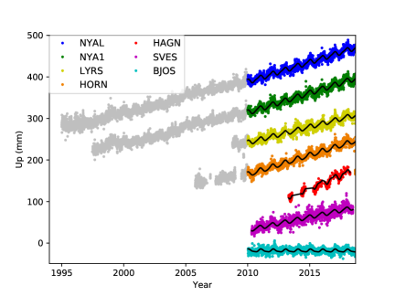
Figure 3: GNSS vertical time series for the Gamit-NMA solutions. The color coded time span is the data period used in this study. The black curves are the model function fitted to this period. The HORN station was moved to a new location in 2009. The time series are shifted with respect to each other to improve readability.

2.4 VLBI

The VLBI station NYALES20 participated in 2183 twenty four hour observing sessions from 1994-10-04 to 2020-10-19. We ran several solutions.

Solution s1 was obtained using the geodetic analysis software Where (see Kirkvik et al., 2017, for more details). VLBI observing sessions were individually analyzed with the following approach: a priori station coordinates were taken from  including the post-seismic deformation models or VTRF2019d (IVS update of ITRF2014) for newer stations. To define the origin and the orientation of the output station position estimates, tight no-net-translation and no-net-rotation with respect to  were imposed. A priori radio source coordinates were taken from the ICRF3 S/X catalog (Charlot, P. et al., 2020) and corrected for the galactic aberration. The source coordinates were not estimated. A priori Earth orientation parameters were taken from the C04 combined EOP series consistent with . The Earth orientation parameters, polar motion, polar motion rate, UTC-UT1, length of day, and celestial pole offsets, were then estimated for each session. In addition, troposphere and clock parameters was estimated.Key parameters for the VLBI solutions are included in Table 2.

Table 2: VLBI analysis strategies.

	Where	pSolve
A priori radio source coordinates	ICRF3 S/X	Solved for
A priori EOP	C04 combined	Solved for
Elevation angle cutoff	0 degree	5 degree
Troposphere mapping function	VMF1	Direct integration
	(Boehm et al., 2006)	using output of
		numerical weather
		model GEOS-FPIT
Solid Earth tide	IERS2010	Elastic
		(Mathews et al., 1997)
Ocean tidal loading	TPXO7.2	FES2014B
Ocean pole tide	IERS2010	IERS2010
Higher order ionosphere	Not applied	Applied

Solution s2 was obtained using VLBI analysis software suite pSolve (http://astrogeo.org/psolve). Source position, station positions, station velocity, sinusoidal position variations at annual, semi-annual, diurnal, semi-diurnal frequencies of all the stations, were estimated as global parameters in a single least square solution using all dual-band ionosphere-free combinations of VLBI group delays from 1980-04-12 to 2020-12-07, in total 14.8 million observations. There are 28 stations that have discontinuities due to seismic events or station repair. These discontinuities and associated non-linear motion was modeled with B-splines with multiple knots, and the B-spline coefficients were treated as global parameters. In addition to global parameters, the Earth orientation parameters, pole coordinates, UT1, their first time derivatives, as well as daily nutation offsets are estimated for each observation session individually. Atmospheric zenith path delay and clock function are modeled with B-splines of the 1st degree with time span 60 and 20 minutes, respectively. A so-called minimum constraints on station positions and velocities and source coordinates were imposed to invert the matrix of the incomplete rank. These constraints require that the net translation and rotation station positions and velocities of a subset of stations be the same as in ITRF2000 catalog and net rotation of the so-called 212 defining sources be the same as in ICRF. It should be noted that s2 solution is independent on the choice of the a priori reference frame, i.e. change in the a priori position does not affect results.

The data reduction model included modeling thermal variation of all antennas, oceanic tidal,     and  loading with one exception, where for station NYALES20 the following  model were used $D_{\rm merra}-D_{\rm merra,svalbard}$. Implying that the a priori model totally ignores mass loading exerted by water mass redistribution in Svalbard.

The VLBI network is small and heterogeneous: different stations participate in different experiments. Therefore, the time series of station position should be treated with a great caution: the estimate of the position change of station X affects the position estimate of station Y because of the use of the net translation and net rotation constraints to solve the system of the incomplete rank. An alternative approach to processing time series is estimation of admittance factor. We assume that the time series of the displacement in question d(t) is present in data as $a\cdot d(t)$ where $a$ is a dimensionless parameter called an admittance factor that is assumed constant for the time period of observations. The admittance factor describes what share of the modeled signal is present in observations.

We noticed that seasonal crustal deformations of NYALES20 positions are periodic but not sinusoidal. The shape of these variations is surprisingly stable with time (See Fig. 4). We decomposed the mass loading signal into four components: seasonal, interannual, linear trend, and residuals. The decomposition was performed in three steps. First, the mass loading time series were filtered with the low-pass Gaussian filter, which provided a coarse interannual signal (IAV$(t)$). Second, the time series were folded of the phase in a form $p=(t-t_{0})/\Delta t$, where $t$ is time, $t_{0}$ is the reference epoch 2000.0, $\Delta t$ is the period (one year), and then smoothed. That provided a coarse estimate of the seasonal signal (SEA$(t)$, blue curve in Fig. 4). Then we adjusted parameters $A$, $B$, $a_{i}$, $s_{i}$ of the decomposition of the loading displacements $D(t)$ described by the Eq 4, using a single least square solution:

$$D_{\rm CMB}(t)={\rm IAV}(t)+{\rm SEA}(p(t))+A+Bt+\varepsilon(t),$$ (4)

where

$${\rm IAV(t)} = \sum_{i}a_{i}B_{i}(t)$$

$${\rm SEA(t)} = \sum_{i}s_{i}B_{i}(p(t)),$$

where $B_{i}$ is the basis spline of the 3rd degree with the pivotal knot $i$.

Fig. 4 illustrates the seasonal component of the loading signal at NYALES20. A thin red line at the plot shows result of the best fit of the sinusoidal signal. However, the sinusoidal model provides a poor fit to the data with errors reaching 40% of the seasonal signal. All constituents of this expansion for NYALES20 are shown in Fig. 5.

In solution s3 we did not estimated annual and semi-annual sinusoidal variations of NYALES20 positions, but estimated admittance factors for the up, east, and north components of the ${\rm IAV}(t)+{\rm SEA}(p(t))$ mass loading time series. In contrast to estimation of sinusoidal variations, the shape and phase of the signal remains fixed when we estimate admittance. The adjusted parameter is the scaling factor of the modeled displacement magnitude. The power of this approach is that it allows us to evaluate quantitatively the amount of the modeled signal in data, and test a statistical hypothesis that all model signal is present in the data.

The results of admittance factor estimation are presented in Table 3 in row ADM_TOT. Then we estimated the admittance factor for the seasonal ${\rm SEA}(p(t))$ and interannual variations ${\rm IAV}(t)$ separately in the s4 solution.

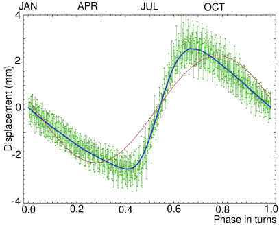
Figure 4: Folded periodic up LWS mass loading displacements of NYALES20 after removal of the slowly varying constituent. The thick blue line shows the estimate of the seasonal constituent. Green dots show the mass loading signal after removal of the interannual constituent. A red thin line shows a sinusoidal fit in a form $a\cos 2\pi\,p+b\sin 2\pi\,p$, where $p$ is the phase of the seasonal signal in turns.

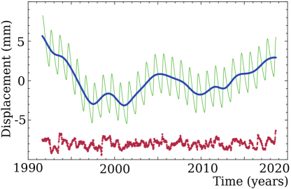
Figure 5: Three constituents of the vertical LWS mass loading at station NYALES20. The thick blue line shows the interannual variation, the green thin line shows the seasonal component, and red dots in the bottom shows the residual signal. The residual signal is artificially shifted by -8mm. The linear trend is removed and not shown.

Table 3: Admittance factors of NYALES20 displacements caused by LWS loading. The first row, ADM_TOT shows the admittance factor estimate from s3 solution of the total mass loading signal. Rows ADM_SEA and ADM_IAV shows estimates of the seasonal and interannual constituents of the loading signal from s4 solution respectively.

Factor	Up	East	North
ADM_TOT	1.38 $\pm$ 0.04	0.62 $\pm$ 0.05	2.05 $\pm$ 0.12
ADM_SEA	1.10 $\pm$ 0.05	0.47 $\pm$ 0.11	6.10 $\pm$ 0.49
ADM_IAV	2.90 $\pm$ 0.07	2.44 $\pm$ 0.11	1.00 $\pm$ 0.15

2.5 Gravimetry/SCG

We use gravity measurements from two  instruments covering the period 1999 to 2018 to estimate gravity change. Gravity measurements from 1999 to 2013 and 2014 to 2018 are collected with C039 and iGrav012 SCG instrument, respectively. The original gravity measurements have a spacing of 1 second, giving a total of approximately 620 million measurements. They are re-sampled every minute using a symmetric numerical Finite Impulse Response (FIR) zero phase low-pass filter with a cut-off at 120 seconds (Wenzel, 1996). Data was then cleaned for outliers and earthquakes. We corrected for the effect of air pressure using the value of -0.422 $\pm$ 0.004 $\mu$Gal/hPa found by Sato et al. (2006a). Both the solid earth and ocean tides are removed from the gravity data by estimating a synthetic tide based on Hartmann & Wenzel (1995) tidal model and a set of tidal parameters. The synthetic tide is estimated using ETERNA 3.4 (Wenzel, 1996).

We also estimated and removed the instrumental drift by comparing to absolute gravity measurements. We estimated a linear drift (using unweighted least squares) by comparing to ten AG measurements (2000, 2001, 2002, 2004, 2007, 2010, twice in 2012, 2014, 2017). The estimated value is -2.74107 $\pm$ 0.17 $\mu$Gal/year. Finally, we re-sampled the data first every 5 minutes and then every 1 hour using a symmetric FIR zero phase filter (cutoffs 1250 sec and 2 hours, respectively) and then to daily values using a flat filter.

2.6 Filtering of Common Mode and elastic loading signal

It is well known that stations in a region can have a spatially correlated signal, a so-called  signal (Wdowinski et al., 1997), and that removal of the  signal can reduce noise in the time series. The  signal could come from the  analysis strategy and from the strategy for reference frame realization. It could come from mismodeled orbit, clocks or EOPs, or through unmodeled large scale hydrology or atmospheric effects. To remove such signal either  filtering,  or regional reference frame realization, can be used. All these methods presuppose that we have stations exposed to the same undesirable  signal. In Arctic areas, we have limited access to nearby stations. All stations on Svalbard are exposed to similar signals from glaciers, using one or several of these stations for removal of the  signal will not only remove the  signal, but also the real elastic signal from snow and ice.

The station BJOS at Bear Island is located 240 km south of Svalbard. The Island is small and surrounded by ocean and the local loading signal from ice and snow is approximately 10% of the signal in Ny-Ålesund (see Tabel 9). It is the closest GNSS station outside Svalbard. Time series of the BJOS station are used to estimate the  signal. Time series for the BJOS station, and hence  filtering, are only included in the solutions computed by the authors (Gamit-NMA, GipsyX-FID and GipsyX-NNR) and not available in the external solutions (SOPAC, JPL, UNR and ITRF).The  filtered time series for the $i$-th station is then:

$$H_{CM}^{i}(t)=H_{GNSS}^{i}(t)-CM(t)=H_{GNSS}^{i}(t)-H_{GNSS}^{BJOS}(t),$$ (5)

where $t$ is the epoch and $H_{GNSS}^{i}$ and $H_{GNSS}^{BJOS}$ is the time series for station $i$ and $BJOS$ respectively.

The  filtering removes the common error signal at the stations as well as real measured signal at BJOS. If the station at Bear Island has an unique unmodelled loading signal not present in other Svalbard stations, this unique signal will be erroneously subtracted also from the other stations.

To  filter a time series where the signal from a loading model is removed, the loading signal for the station(s) used in the  filtering has to be removed as well. In our case, the loading signal was subtracted both for the BJOS time series before computing the  signal and for the other Svalbard time series before the  filtering. The final Svalbard time series are cleaned for both the regional  signal over Svalbard and Bear Island and the estimated load signal. The  filtered time series for station $i$ is then:

$$H_{CM,L}^{i}(t)=H_{GNSS}^{i}(t)-H_{L}^{i}(t)-CM(t),$$ (6)

where $t$ is the epoch, $H_{GNSS}^{i}$ is the observed time series, $H_{L}^{i}$ is the estimated loading signal, and $CM$ is the common mode signal. As described earlier, we use the time series from BJOS to estimate the  signal, but since we remove the estimated loading signal from the time series, we have to remove the loading signal from BJOS time series before computing the  signal. Therefore, we get

$$H_{CM,L}^{i}(t)=H_{GNSS}^{i}(t)-H_{L}^{i}(t)-(H_{GNSS}^{BJOS}(t)-H_{L}^{BJOS}(t)).$$ (7)

2.7 Isolating the elastic signal from glacier and snow

The signal in $H_{CM,L}(t)$ (Eq. 7) includes all vertical motions not accounted for in the loading models or  filtering, e.g., unmodeled loading, , tectonics, and noise. Assuming that the  and the tectonic component are linear, the left hand side can be written $H_{CM,L}(t)=LIN(t)+\varepsilon(t)$, where $LIN$ is the linear part and $\varepsilon$ contains the noise. The noise includes unmodeled loadings, but also station dependent effects like multipath, atmospheric effects, not use of individual antenna calibration, and thermal expansion of antenna monument. Possible unique unmodelled signal from BJOS will also map into the noise term. Splitting the load signal into a signal from glacier and snow, $H_{GS}$, and other non tidal loadings, $H_{NTL^{*}}$, we can rewrite Eq. 7 into:

$$LIN^{i}(t)+H_{GS}^{i}(t)+\varepsilon(t) = H_{GNSS}^{i}(t)-H_{NTL^{*}}^{i}(t)$$ (8)

$$- \left(H_{GNSS}^{BJOS}(t)-H_{NTL^{*}}^{BJOS}(t)\right.$$

$$-\left.H_{GS}^{BJOS}(t)\right),$$

i.e. we have isolated the linear part and the elastic signal from glaciers and snow as a sum of known terms.

3 Results and Discussion

The vertical component of the different GNSS solutions in Ny-Ålesund and Bear Island as well as the  signal are included in Table 4. In addition, the Where results (Solution s1) from the NYALES20 VLBI antenna and the  in Ny-Ålesund are included. Some of the time series are plotted in Fig. 6. The horizontal components of the different GNSS solutions are included in Appendix, Table 8. The loading signals for all the different loading models are included in the Appendix, Table 9.

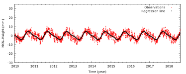
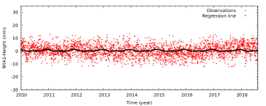
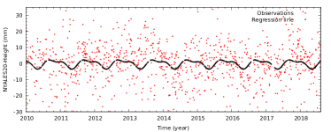
Figure 6: A selected set of detrended time series for Svalbard. The time series are: GipsyX-NNR for NYA1 (upper left),  (, ,  including the glaciers and snow) signal in Ny-Ålesund (middle left), the GipsyX-NNR time series for NYA1 after removal of  and CM filtering (lower left), GipsyX-NNR for BJOS (upper right), gravity from the  in Ny-Ålesund (middle right) and the NYALES20 Where solution (lower right). The gravity values are converted to millimeter using the convertion ratio -0.24 $~{}\mu$Gal/mm (Mémin et al., 2012).

Table 4: Trend, annual- and semi- signal in Ny-Ålesund and Bear Island. The parameters are estimated trend and annual signal estimated using Eq. 3). The results are for different GNSS solutions, VLBI, SCG and NTL in Ny-Ålesund and Bear Island. In the VLBI time series a pure white noise model is assumed. The gravity values ($*$) are converted to millimeter using the convertion ratio -0.24 $~{}\mu$Gal/mm from Mémin et al. (2012). CM is the CM filtered time series described in Section 2.6. NTL is the sum of non tidal elastic loading signal from ATM, NTO and LWS including the load from snow and glacier from the CMB model.

Station		Trend	Annual signal		Semi-annual signal
		(mm/yr)	Amp. (mm)	Pha. (deg)	Amp. (mm)	Pha. (deg)
NYA1	Gamit-SOPAC	9.61 +/- 0.62	6.28 +/- 0.64	-51.3 +/- 5.8	1.71 +/- 0.44	107.1 +/- 14.6
	Gamit-NMA	9.62 +/- 0.62	5.80 +/- 0.64	-13.0 +/- 6.3	1.42 +/- 0.44	57.6 +/- 17.2
	GipsyX-FID	9.49 +/- 0.69	3.05 +/- 0.70	-45.7 +/- 13.0	1.05 +/- 0.45	123.1 +/- 23.2
	GipsyX-NNR	9.26 +/- 0.67	2.96 +/- 0.69	-27.4 +/- 13.1	0.91 +/- 0.42	134.0 +/- 24.8
	GipsyX-UNR	9.27 +/- 0.67	2.91 +/- 0.69	-27.6 +/- 13.3	0.91 +/- 0.42	135.2 +/- 24.8
	GipsyX-JPL	9.59 +/- 0.65	3.36 +/- 0.66	-12.9 +/- 11.1	1.08 +/- 0.43	161.5 +/- 21.9
	ITRF2014	9.00 +/- 0.95	4.05 +/- 0.75	-36.2 +/- 10.5	1.08 +/- 0.47	157.5 +/- 23.6
	Gamit-NMA (CM)	9.55 +/- 0.36	4.07 +/- 0.38	-47.5 +/- 5.4	0.66 +/- 0.26	113.1 +/- 21.3
	GipsyX-FID (CM)	9.80 +/- 0.31	2.84 +/- 0.34	-54.0 +/- 6.8	0.86 +/- 0.24	136.5 +/- 15.9
	GipsyX-NNR (CM)	9.86 +/- 0.35	2.91 +/- 0.38	-58.2 +/- 7.4	0.82 +/- 0.27	127.9 +/- 18.1
NYAL	Gamit-SOPAC	9.41 +/- 0.61	6.24 +/- 0.63	-56.6 +/- 5.8	1.96 +/- 0.44	105.8 +/- 12.7
	Gamit-NMA	9.57 +/- 0.67	5.22 +/- 0.69	-12.9 +/- 7.6	1.75 +/- 0.48	64.3 +/- 15.4
	GipsyX-FID	9.34 +/- 0.67	3.45 +/- 0.74	-59.4 +/- 12.1	1.16 +/- 0.48	122.1 +/- 22.5
	GipsyX-NNR	9.14 +/- 0.66	3.19 +/- 0.68	-39.9 +/- 11.9	1.12 +/- 0.45	124.2 +/- 21.6
	GipsyX-UNR	9.13 +/- 0.65	3.17 +/- 0.66	-39.9 +/- 11.8	1.11 +/- 0.44	125.5 +/- 21.6
	GipsyX-JPL	9.39 +/- 0.65	3.44 +/- 0.66	-27.7 +/- 10.9	1.17 +/- 0.44	153.2 +/- 20.8
	ITRF2014	9.34 +/- 0.98	4.37 +/- 0.78	-47.7 +/- 10.1	1.17 +/- 0.50	156.1 +/- 23.0
	Gamit-NMA (CM)	9.52 +/- 0.35	3.60 +/- 0.37	-52.9 +/- 5.9	0.96 +/- 0.26	102.8 +/- 15.3
	GipsyX-FID (CM)	9.67 +/- 0.33	3.34 +/- 0.38	-63.9 +/- 6.5	1.17 +/- 0.28	122.9 +/- 13.4
	GipsyX-NNR (CM)	9.75 +/- 0.34	3.45 +/- 0.36	-68.1 +/- 6.0	1.11 +/- 0.26	120.6 +/- 13.4
NYALES20	Where	8.87 +/- 0.17	2.62 +/- 0.80	-67.3 +/- 17.9	1.14 +/- 0.81	77.3 +/- 31.5
NYAL-SCG		∗2.52 +/- 0.64	∗14.38 +/- 0.67	-83.8 +/- 2.7	∗3.92 +/- 0.47	60.6 +/- 6.8
Ny-Ålesund	NTL	0.92 +/- 0.30	4.00 +/- 0.32	-82.5 +/- 4.6	1.21 +/- 0.22	111.3 +/-10.3
BJOS	Gamit-NMA	0.10 +/- 0.54	3.30 +/- 0.55	32.6 +/- 9.5	1.14 +/- 0.38	33.6 +/- 18.4
	GipsyX-FID	-0.27 +/- 0.62	0.90 +/- 0.47	21.2 +/- 27.3	0.62 +/- 0.32	45.5 +/- 27.5
	GipsyX-NNR	-0.47 +/- 0.59	1.63 +/- 0.58	46.1 +/- 19.6	0.57 +/- 0.30	-54.0 +/- 27.6
Bear Island	NTL	-0.04 +/- 0.31	1.99 +/- 0.32	-107.7 +/- 9.1	0.38 +/- 0.18	100.1 +/-25.3

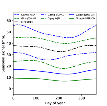
Figure 7: Seasonal signal in Ny-Ålesund (NYA1). The left panel shows the sum of the annual and semi-annual sinusoidal signal for the time series, the right panel shows the same results relative to the NTL signal (ATM, NTO, LWS including the glaciers and snow). The upper most five curves are from time series analysis of the raw time series. The sixth and seventh curves are CM-filtered time series. The bottom curve of the left panel is the estimated NTL signal. The curves are shifted with respect to each other to improve readability.

3.1 Determination of the loading annual signal

As shown in Kierulf et al. (2009b) the uplift in Ny-Ålesund varies from year to year. Consequently, trends from different time periods can not be compared directly. We have chosen to use the time interval 2010 until 2018 for time series analysis, except for the  time series that ended in 2014. The estimated uplift for the Ny-Ålesund stations agree below the uncertainty level.

The annual signal in Ny-Ålesund varies between the solutions both in phase and amplitude (Table 4, Table 8 and Fig. 7). This implies that the choice of GNSS analysis strategy has a noticeable impact on the estimated seasonal variations. Martens et al. (2020) found similar differences in the estimated annual signal when they compared GNSS time series, in US and Alaska, based on different analysis strategies. Such variations make direct geophysical interpretation of the periodicity in GNSS time series difficult.

The measured vertical annual signal (Table 4) is smaller than the estimated  signal for the GipsyX solutions and larger than the estimated  signal for the Gamit solutions. The phase of the GNSS solutions are delayed relative to the  signal with between 30 and 70 degrees (corresponding to a delay between one and two and a half months) in Ny-Ålesund.

The -filtered solutions are closer to the expected signal from  and we have less differences between the GipsyX and Gamit solutions, see Fig. 7. The annual signal found with the Where software for VLBI has a smaller amplitude, but the phase is close to the phase estimated from the loading modeling.

The phase of the gravity signal in Ny-Ålesund is close to the phase of the loading models. The annual amplitude in gravity is $3.45~{}\mu Gal$. For a spherical and compressible Earth model the elastic gravity variations can be converted to vertical position variations using a ratio of -0.24 $~{}\mu$Gal/mm (Mémin et al., 2012). Using this ratio we got an yearly amplitude of 14.4 mm. This is much larger than the estimated annual loading signal of around 4.0 mm in Ny-Ålesund. However, the gravity variations also depends on the direct gravitational attraction. Mémin et al. (2012) discussed how the location of the load affect the ratio between gravity and uplift. Both the distance to and the relative height of the load have an impact. The large annual signal implies mass changes at locations with negative relative heights close to the station.

The -instrument in Ny-Ålesund gives a combined signal from three glacier related factors. The visco-elastic response from past ice mass changes, the immediate elastic response of the ongoing ice mass changes, and the direct gravitational attraction from the ongoing ice mass changes on the glaciers (see Mémin et al., 2014; Breili et al., 2017). The two latter have a clear influence on the annual signal. In addition, soil moisture and accumulated snow close to and mainly below the gravimeter, have a much stronger effect on gravity than on displacements.

Quantifying the gravity signal from these nearby hydrological factors are demanding and out of the scope of this paper. However, they, as well as glaciers, are forced by temperature and precipitation. We assume that they are in phase with the elastic uplift signal. A gravimeter measures gravity changes directly, while VLBI and GNSS evaluate site positions from analysis of observations at a network, and a position estimate of a given station in general depends on measurements at other stations of the network. The phase of the  time series is therefore an independent measure of the variations in Ny-Ålesund and the result coincides with the results from the other techniques.

3.2 Determination of the loading admittance factors

We found the admittance factor from VLBI solutions for the seasonal vertical displacement does not deviate from 1.0 at a $2\sigma$ level, i.e. the  signal is fully recovered from the data. At the same time the departure of the admittance factor from 1.0 for the horizontal loading components implies there is a statically significant discrepancy between the computed loading signal and the data. It should be noted that the magnitude of the seasonal signal in North direction is only 0.15 mm and the signal itself is just too small to be detected. The admittance factor for the interannual signal is significantly different from 1.0, which indicates that the loading signal alone cannot explain it.

We made an additional analysis to find the admittance factor for the glacier and snow loading signal at the GNSS stations in Svalbard. We computed mass loading for all the GNSS stations in Svalbard and fitted it to the GNSS time series using reciprocal formal uncertainties as weights. Then we computed the $\chi^{2}$ per degree of freedom of the fit and scaled variances of admittance factor estimates by this amount. Table 5 shows the estimates of the admittance factor from the differenced GNSS time series using Eq. 8. Similar to the VLBI case, the admittance is very close to 1.0 for the vertical seasonal signal (row “All”) and it is far away from 1.0 for the interannual signal and the horizontal signal.

Two factors may cause poor modeling of the interannual signal. First, calving and frontal ablation are not included in the  model, and therefore, lacks this contribution. Second, other loadings, for instance non-tidal ocean loading may contribute. The seasonal signal has a very specific time dependence pattern, and the approach of admittance factor estimation exploits the uniqueness of this pattern, while the pattern of the interannual signal is more general.

Table 5: Admittance factors for the vertical component of GNSS station in Svalbard caused by the glacier and snow loading. ADM_SEA and ADM_IAV show estimates of the seasonal and interannual admittance factors.

Station	ADM_SEA	ADM_IAV
SVES	0.94 $\pm$ 0.15	0.04 $\pm$ 0.13
NYAL	1.33 $\pm$ 0.18	0.03 $\pm$ 0.17
NYA1	1.01 $\pm$ 0.18	0.19 $\pm$ 0.16
LYRS	0.95 $\pm$ 0.18	-0.11 $\pm$ 0.21
HORN	1.35 $\pm$ 0.16	0.25 $\pm$ 0.17
All	1.12 $\pm$ 0.07	0.11 $\pm$ 0.07

The analysis of the admittance factors give several important results in addition to the very good agreement between the different estimated vertical seasonal components. Analysis of observations shows that the  model provides prediction of the vertical mass loading with 1-$\sigma$ errors of 5%, which corresponds to 0.1 mm. We have a bias wrt to the model of 0.2 $\pm$ 0.1 mm, and this bias is not statistically significant at a 95% level (2 sigma). We conclude that analysis of the data from two totally independent techniques, VLBI and GNSS, proves there is no statistically significant deviation at a 95% significance level between the seasonal vertical mass loading signal based on the  model and observations of both techniques.

3.3 Geodynamical interpretation

To study the time series ability to capture the loading signal from glaciers and snowpack changes, we used the  filtered time series. Other known loading signals were removed using Eq. 8. To have more robust time series, in the following discussion, we have used averaged GNSS time series. The averaged time series are the weighted mean of the daily values from the Gamit-NMA, the GipsyX-NNR and the GipsyX-FID solutions. The annual periodic signal and the linear rate for the time series in Eq. 8 are included in Table 6 together with the elastic signal from glaciers and snow. Detailed results for the individual GNSS solutions are included in the Appendix, Table 10.

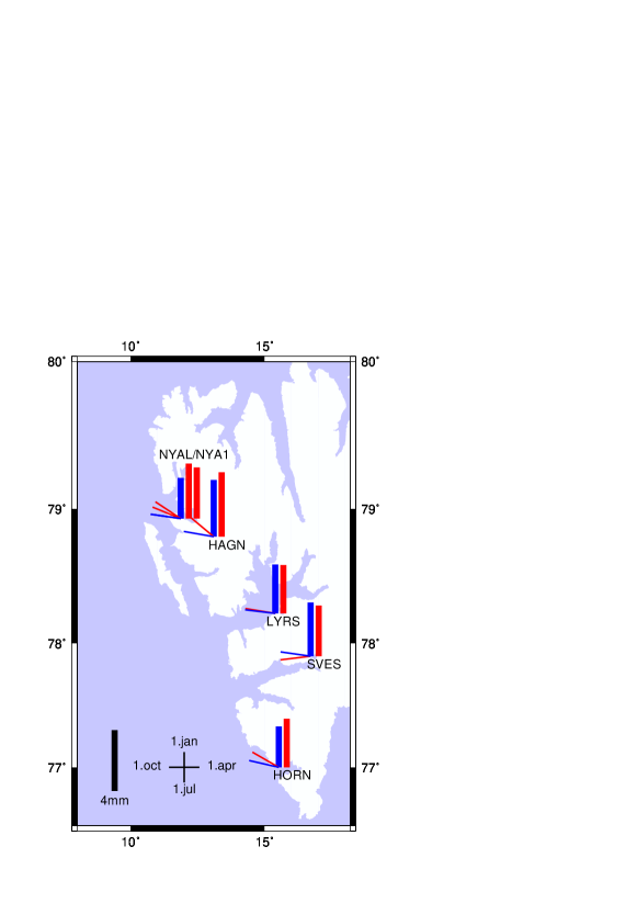
Figure 9: Annual signal for GNSS stations in Svalbard. The bars are the amplitude and the vectors are the phase. Blue is from the loading prediction from glaciers and snow red is from the GNSS stations.

The amplitudes of the estimated loading signal from glaciers and snowpack vary with latitude and longitude and depend on the amount of surrounding glaciers and land masses (see Fig. 9). The station HAGN in the middle of the glacier Kongsvegen has the largest estimated annual loading signal, while the westernmost stations NYAL/NYA1 and HORN have the smallest. The GNSS stations SVES and LYRS are located in central parts of Svalbard and here the measured vertical annual signal agrees with the estimated loading signal at the uncertainty level. For the stations closest to the west coast NYAL, NYA1 and HORN the measured amplitudes are slightly larger than expected from the variations in glaciers and snow ($\sim 0.7$ mm, $\sim 1.0$ mm and $\sim 0.5$ mm resp.). Although the admittance factor for all stations combined show very good agreement for the seasonal component, the admittance factor for individual stations in Ny-Ålesund and Hornsund are slightly above one, implying that the observed amplitude is somewhat larger than the prediction from the  model.

The larger vertical amplitude at NYAL, NYA1 and HORN might be due to lower precision of the  models in areas with more variable coastal climate, changes in groundwater and surface hydrology, and seasonal variability in calving/frontal ablation of glaciers. Especially, calving is assumed to be seasonally dependent with higher incidents during summer (when ice flows faster). This may explain a higher observed amplitude in areas like Ny-Ålesund and Hornsund, which have a lot of nearby large calving glaciers. However, the deviation of admittance factors from 1.0 for these stations is still within $2\sigma$ of the statistical uncertainty. Longer time series are needed to establish whether there is a statistically significant deviation of observations from the model for these individual stations.

The phase of the vertical loading signal from glaciers and snow varies with only a few days over Svalbard, and corresponds to a maximal value after the end of the melting season, in mid-October. The phase of the GNSS time series agrees with the glaciers and snow signal from the  models within a few weeks.

The predicted horizontal seasonal signal is smaller. It is around 0.2 mm in the north component for all locations except HORN. HORN is located in the south of Svalbard with the majority of glaciers located to the north. Consequently the north amplitude is larger, 0.7 mm. The other stations have glaciers both to the north and to the south and the loading signals are cancelled out. The east annual signal varies from 0.7 mm (NYAL, NYA1) to 0.0 mm (SVES), depending on their locations relative to the glaciers.

We see that the estimated annual signal for the GNSS stations NYA1, HAGN, LYRS and HORN agree at 2-sigma level in the east component. HORN is capturing the larger north annual signal for this location. However, the small north signals for the other stations are too small to be detected. LYRS and SVES have a large north annual signal, 1.1 mm resp. 2.3 mm larger than expected loading signal. We have not established the origin of this discrepancies. Possible reasons are uneven thermal expansion of the antenna monument (steel mast) and artifacts of the atmosphere model. We will investigate these signals in the future.

Our CMB model is limited by Svalbard archipelago. Glacial loading at other islands, such as Iceland and Greenland, can bring a noticeable contribution. Using Green’s function from the ocean tide loading provide of Scherneck (1991), assuming 100 Gt seasonal ice cycle on Greenland (see figure 6 in Bevis et al., 2012), and the average distance from Greenland to Svalbard of 800 km, we get coarse estimate of the the amplitude of mass loading signal Svalbard due to glacier in Greenland: 0.38 mm. In order to get a more refined estimate of the magnitude of such a contribution, we used Loomis et al. (2019) mascon solution for Greenland for 2008 from processing GRACE mission. The mascon for Greenland at a regular grid $0.5^{\circ}\times 0.5^{\circ}$ is provided with a monthly resolution in the height of the column of water equivalent that covers the entire land and is zero otherwise. The mascon excludes the contribution of the atmosphere and ocean but retains the contribution of land water, snow, and ice storage.

We have converted the height of the column of water equivalent to surface pressure and computed the mass loading from the mascon using the same approach as we used for computing atmospheric and land water storage loading using spherical harmonic transform of degree/order 2699. Since MERRA2 land water storage model covers Greenland, we computed mass loading two times: the first time using the total surface pressure from the mascon and the second time after subtracting the pressure anomaly from MERRA2. In the latter case the resulting mass loading signal provides a correction to the mass loading from MERRA2 model for the contribution of glacier derived from GRACE data analysis since MERRA2 has large errors of modeling glacier dynamics. The results are shown in Figure 8 after removal linear trend. The residual signal has amplitude 0.15 mm and is in phase with the mass loading signal from Svalbard glacier while the total signal has amplitude 0.28 mm. This estimate agrees remarkably well with our coarse estimate. Accounting for the contribution of glacier mass loading using GRACE data reduces the admittance factor from 1.10 to 1.04 for the seasonal vertical component of the VLBI solution.

We exercise a caution in results of processing GRACE data, A thorough analysis of systematic errors of mass loading signal from GRACE mascon solution requires significant efforts and is beyond the scope of the present manuscript. However, our estimates shows that the contribution of glaciers in Greenland is not dominated and its accounting improves the agreement of the CMB model with VLBI and GNSS observations.

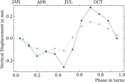
Figure 8: The seasonal contribution of glaciers in Greenland to the vertical displacement of NYALES20 after removal of the slowly varying constituent from processing GRACE data. The green line shows the total contribution, the shadowed blue line shows the residual contribution after subtraction of land water storage pressure from MERRA2 model. The horizontal axis is a phase of the seasonal signal in phase turns.

Table 6: Vertical rate and annual signal for GNSS stations in Svalbard. GS are the elastic loading signal from ice and snow. GNSS-CM is the time series using Eq. 8. Max uplift is the date of the maximum value for the annual signal.

Station		Trend	Amp.	Pha.	Max up
		mm/yr	mm	deg	date
Up:
NYA1	GNSS-CML	9.74 +/- 0.27	3.37 +/- 0.29	-56.5 +/- 5.0	3 Nov.
	GS	0.93 +/- 0.03	2.66 +/- 0.03	-81.8 +/- 0.6	9 Oct.
NYAL	GNSS-CML	9.57 +/- 0.27	3.63 +/- 0.29	-67.9 +/- 4.6	23 Oct.
	GS	0.93 +/- 0.03	2.66 +/- 0.03	-81.8 +/- 0.6	9 Oct.
HAGN	GNSS-CML	11.95 +/- 0.56	4.28 +/- 0.65	-50.2 +/- 8.6	10 Nov.
	GS	1.81 +/- 0.04	3.73 +/- 0.04	-80.1 +/- 0.7	10 Oct.
LYRS	GNSS-CML	8.16 +/- 0.42	3.21 +/- 0.45	-80.8 +/- 8.0	10 Oct.
	GS	0.83 +/- 0.03	3.21 +/- 0.03	-83.2 +/- 0.6	7 Oct.
SVES	GNSS-CML	6.21 +/- 0.45	3.37 +/- 0.47	-96.8 +/- 7.9	23 Sep.
	GS	0.86 +/- 0.04	3.53 +/- 0.04	-81.9 +/- 0.6	8 Oct.
HORN	GNSS-CML	9.45 +/- 0.27	3.21 +/- 0.30	-60.0 +/- 5.3	31 Oct.
	GS	1.93 +/- 0.03	2.69 +/- 0.03	-77.0 +/- 0.6	13 Oct.
North:
NYA1	GNSS-CML	14.98 +/- 0.09	0.24 +/- 0.09	39.6 +/- 21.1	9 Feb.
	GS	0.56 +/- 0.01	0.17 +/- 0.01	-72.0 +/- 1.0	18 Oct.
NYAL	GNSS-CML	14.84 +/- 0.12	0.47 +/- 0.12	-89.5 +/- 14.9	1 Oct.
	GS	0.56 +/- 0.01	0.17 +/- 0.01	-72.0 +/- 1.0	18 Oct.
HAGN	GNSS-CML	14.73 +/- 0.36	0.83 +/- 0.34	147.7 +/- 22.2	29 May.
	GS	0.53 +/- 0.01	0.05 +/- 0.01	-49.1 +/- 3.4	11 Nov.
LYRS	GNSS-CML	14.47 +/- 0.16	1.19 +/- 0.17	63.6 +/- 8.2	5 Mar.
	GS	0.24 +/- 0.01	0.06 +/- 0.01	84.4 +/- 3.6	26 Mar.
SVES	GNSS-CML	14.49 +/- 0.33	2.55 +/- 0.33	35.4 +/- 7.3	4 Feb.
	GS	0.19 +/- 0.01	0.24 +/- 0.01	89.0 +/- 1.2	31 Mar.
HORN	GNSS-CML	13.20 +/- 0.14	1.02 +/- 0.14	91.7 +/- 8.0	2 Apr.
	GS	-0.43 +/- 0.01	0.73 +/- 0.01	101.6 +/- 0.7	13 Apr.
East:
NYA1	GNSS-CML	10.24 +/- 0.08	0.42 +/- 0.09	18.6 +/- 11.8	18 Jan.
	GS	-0.07 +/- 0.01	0.64 +/- 0.01	98.3 +/- 0.8	9 Apr.
NYAL	GNSS-CML	10.01 +/- 0.08	0.16 +/- 0.07	-59.1 +/- 25.0	1 Nov.
	GS	-0.07 +/- 0.01	0.64 +/- 0.01	98.3 +/- 0.8	9 Apr.
HAGN	GNSS-CML	12.65 +/- 0.32	0.66 +/- 0.29	151.4 +/- 23.9	2 Jun.
	GS	0.32 +/- 0.01	0.40 +/- 0.01	94.5 +/- 0.9	5 Apr.
LYRS	GNSS-CML	12.48 +/- 0.17	0.35 +/- 0.15	77.7 +/- 23.5	19 Mar.
	GS	0.08 +/- 0.01	0.27 +/- 0.01	95.9 +/- 1.1	7 Apr.
SVES	GNSS-CML	15.71 +/- 0.27	0.76 +/- 0.26	31.9 +/- 18.8	1 Feb.
	GS	-0.17 +/- 0.01	0.07 +/- 0.01	117.7 +/- 2.5	29 Apr.
HORN	GNSS-CML	11.56 +/- 0.11	0.45 +/- 0.11	51.2 +/- 13.8	20 Feb.
	GS	-0.31 +/- 0.01	0.32 +/- 0.01	106.4 +/- 0.9	17 Apr.

3.4 CMB model and time series

In the previous section we examined how the different GNSS time series were able to capture the elastic loading signal from local ice and snow changes. In this paragraph we will discuss the effect of removing the loading signal from the time series, both on the unfiltered time series and the  filtered time series. We will in particular look at the effect of replacing the global hydrological model with a regional  model. In the discussion we used an averaged time series from the GNSS solutions; Gamit-NMA, GipsyX-FID and GipsyX-NNR. Due to limited observations during winter the HAGN time series are not directly comparable with the other time series and therefore not included in this discussion.

We have used time series where no loading models where removed and two time series with slightly different loading time series removed ($L_{1}$, $L_{2}$). The first loading model, $L_{1}$, is the sum of the loadings from ,  and the total  signal from the merra2 model. The second loading model, $L_{2}$, equlas $L_{1}$ except that the regional  signal in merra2 is replaced with the glacier and snow signal in the  model using Eq. 2.

$H_{GNSS}-L_{i}$ contains the unmodeled signal in the GNSS time series after removing the modeled loadings, $L_{i}$. The signal can be presented as a sum of linear trend (from e.g., GIA and tectonics) and noise including unmodeled loading signals. I.e. $H_{GNSS}(t)-L_{i}(t)=LIN(t)+\varepsilon(t)$. Also the  filtered time series ($H_{CM}$, Eq. 6) and the  filtered time series where the loading signal is removed ($H_{CM,L_{i}}$, Eq. 7) can be presented as a sum $LIN(t)+\varepsilon(t)$. To examine the quality of the time series using different filtering and loading models we estimate the  and annual signal in the noise time series $\varepsilon(t)$. The annual signal in $\varepsilon(t)$ is the remaining annual signal after removing the loading model $L_{i}$. A large annual signal in $\varepsilon(t)$ indicate that we have remaining unmodelled periodic signal in the time series after removing load $L_{i}$. The  is a measure of the remaining noise in the time series. The results for the averaged time series are included in Table 7. Results for the individual solutions are included in Table 11 in the Appendix.

Table 7: Yearly amplitude and RMS in the time series. In each column the three parameters are amplitude of yearly signal in mm,  of the time series in mm and changes in  relative to the unfiltered time series in percent. The numbers are in mm. $H_{GNSS}$, $L_{i}$ and $H_{CM,L_{i}}$ are explained in the text.

Station	$H_{GNSS}$	$H_{GNSS}-L_{1}$	$H_{GNSS}-L_{2}$	$H_{CM}$	$H_{CM,L_{1}}$	$H_{CM,L_{2}}$
BJOS	1.3 / 4.9( 0%)	2.9 / 4.1( -16%)	3.0 / 4.1( -16%)
NYA1	3.8 / 4.6( 0%)	3.7 / 4.0( -13%)	3.7 / 3.9( -16%)	3.4 / 4.7( 2%)	2.5 / 4.5( -3%)	1.5 / 4.4( -4%)
NYAL	3.6 / 4.6( 0%)	3.1 / 4.1( -12%)	3.0 / 3.9( -15%)	3.4 / 4.7( 3%)	2.5 / 4.5( -3%)	1.3 / 4.4( -4%)
LYRS	3.0 / 6.8( 0%)	2.4 / 6.3( -8%)	2.9 / 6.2( -10%)	2.9 / 6.7( -1%)	1.7 / 6.6( -3%)	0.6 / 6.6( -4%)
SVES	2.5 / 6.5( 0%)	1.7 / 5.8( -9%)	2.8 / 5.7( -11%)	2.9 / 6.3( -2%)	1.5 / 6.1( -5%)	1.1 / 6.0( -7%)
HORN	3.3 / 4.7( 0%)	3.3 / 4.1( -14%)	3.4 / 3.8( -20%)	3.0 / 4.7( -0%)	2.4 / 4.5( -5%)	1.0 / 4.3( -9%)

We see that removal of the loading signal reduce the  values on average by 11%, while replacing the regional hydrological signal with a  model reduce the  with 13%. The improvements for the  filtered time series are less, 4% and 6%, respectively. The removal of the  eliminates part of the elastic loading signal, and this may explains the lower reduction for these series. Both for the unfiltered and the  filtered time series the  are reduced with 2–3 % when we replace the regional signal in the merra2 with the glacier and snow signal from the  model. The  are very little affected by the  filtering (4th vers. 1st column in Table 7).

Removing the  (,  and  including the glaciers and snow) from the observed time series have an effect on the daily noise scatter (), but very little effect on the annual signal. This implies that removal of the  reduces the daily scatter in the GNSS time series. It also implies that the periodic signal is dominated by other factors. As we saw in Section 3 this annual signal depends on the analysis strategy. We conclude that we have an analysis strategy dependent effect in the periodic signal.

The amplitude of the time series is reduced after the  filtering. The amplitude of the annual signal in the  filtered time series using load models $L_{1}$ is reduced to $2.1$ mm. The largest effects are when we use load model $L_{2}$ and the  filtered time series. For this solution the averaged annual loading signal is $1.1$ mm, one third of most other combinations of filtering and loading models.

For the horizontal components including  filtering and removing the NTL affects the RMS only marginaly. The amplitude of the horizontal seasonal signal reduces from on average 0.6 mm to 0.4 mm for NYAL, NYA1 and HORN when both CM filtering and NTL loadings are removed. The stations LYRS and SVES have much larger amplitudes and no improvements after filtering.

Note, the glacier model used in this study is not able to capture glacier dynamics like continuous flow of ice towards the glacier front, or more dramatic phenomena such as glacier surging (see e.g., Morris et al., 2020; Dunse et al., 2015). These dynamic effects provide a significant contribution to the total glacier mass balance and uplift, especially, on time scales from years and longer (see Kierulf et al., 2009b, for more on the effect of glacier dynamics on the uplift). The linear elastic uplift signal from the  models is not sufficient to fully describe the elastic uplift from ice and snow changes over longer time scales.

4 Conclusions

In the introduction two questions were asked: (1) How well do GNSS and VLBI capture the seasonal loading signal from glaciers and snow on Svalbard? (2) Will refining the  models with a  model improve the loading predictions? To answer these questions a network of seven permanent GNSS stations were analyzed with different analysis strategies and softwares. The different time series were studied and compared with loading predictions from , ,  including glaciers and snow.

We found large discrepancies between the different analysis strategies, both in phase and amplitude, while the estimates of long-term trend were more consistent. This implies that a direct geophysical interpretation of raw GNSS time series is problematic. To overcome this problem, we performed  filtering utilizing the data from the nearby station at Bear Island. The elastic loading signal was removed from the time series before the  filtering. The  filtered time series gave a much better agreement. This confirmed our initial conjecture that the origin of the discrepancies in the raw time series are due to differences in the analysis strategy in the GNSS data processing. The agreement of  filtered time series strengthened our confidence that we investigated a real geophysical signal, and not artifacts of data analysis.

We have decomposed the  signal into the seasonal and interannual signals, and estimated admittance factors from VLBI data and GNSS  filtered time series. The admittance factors estimates from vertical seasonal constituents for both techniques do not deviate from 1.0 at a $2\sigma$ level. Therefore, we conclude that the entire mass loading signal is present in data from totally independent technique at a statistical significance level of 95%. The $1\sigma$ uncertainty of admittance factors corresponds to 0.1 mm. This implies that by using the CMB model we can predict seasonal vertical mass loading displacements on Svalbard with the same level of accuracy, and that predicted errors are less than the observation errors. The interannual loading signal was not recovered from observations. Further work is required to explain these discrepancies. However, since calving and frontal ablation are not included in the  model, they may contribute to these discrepancies.

We saw a significant reduction of residuals after subtraction of the  mass loading displacement. The annual amplitude was reduced from $2.1$ mm to $1.1$ mm in the  filtered time series. Subtraction of the  loading had a negligible impact on the unfiltered time series. This provides a strong evidence that  filtering is necessary to reveal local periodic signals when millimeter accuracy is required.

Data availability

The GNSS data from Hornsund (HORN) is provided by the Institute of Geophysics of the Polish Academy of Sciences (IG PAS). Time series from SOPAC, JPL and UNR were used in the study. GNSS time series and SCG data is available from the authors. The NTL time series are avialable from http://massloading.net. Distributed time series of climatic mass balance were extracted from the dataset described in van Pelt et al. (2019).

Appendix A Tables

Table 8: Trend and annual signal in Ny-Ålesund and Bear Island. The parameters are estimated trend and annual signal estimated using Eq. 3) for the North and East components.

Station		North			East
		Trend	Amp.	Pha.	Trend	Amp.	Pha.
		mm/yr	mm	deg	mm/yr	mm	deg
NYA1	Gamit-SOPAC	14.83 +/- 0.12	0.26 +/- 0.11	-11.5 +/- 22.7	10.27 +/- 0.12	1.04 +/- 0.12	-6.0 +/- 6.7
NYA1	Gamit-NMA	14.97 +/- 0.11	0.44 +/- 0.11	-61.8 +/- 14.0	10.46 +/- 0.10	0.61 +/- 0.10	-33.2 +/- 9.6
NYA1	GipsyX-FID	15.00 +/- 0.13	0.67 +/- 0.13	-121.4 +/- 11.4	10.19 +/- 0.12	1.19 +/- 0.12	6.4 +/- 5.8
NYA1	GipsyX-NNR	15.01 +/- 0.13	0.63 +/- 0.13	-116.2 +/- 11.6	10.20 +/- 0.11	1.08 +/- 0.12	15.1 +/- 6.1
NYA1	GipsyX-UNR	14.93 +/- 0.13	0.64 +/- 0.13	-113.7 +/- 11.6	10.30 +/- 0.11	1.06 +/- 0.12	16.7 +/- 6.4
NYA1	GipsyX-JPL	14.67 +/- 0.14	0.78 +/- 0.14	-108.4 +/- 10.2	10.31 +/- 0.13	0.85 +/- 0.13	27.7 +/- 8.9
NYA1	ITRF2014	14.46 +/- 0.17	0.73 +/- 0.14	-83.2 +/- 10.7	10.40 +/- 0.18	1.02 +/- 0.15	2.8 +/- 8.2
NYA1	Gamit-NMA (CM)	14.97 +/- 0.09	0.44 +/- 0.09	20.1 +/- 11.9	10.50 +/- 0.10	0.41 +/- 0.10	-37.2 +/- 14.1
NYA1	GipsyX-FID (CM)	14.98 +/- 0.10	0.29 +/- 0.10	18.1 +/- 19.3	10.23 +/- 0.09	0.41 +/- 0.09	12.7 +/- 13.0
NYA1	GipsyX-NNR (CM)	15.00 +/- 0.09	0.34 +/- 0.10	31.1 +/- 16.1	10.24 +/- 0.08	0.38 +/- 0.09	18.4 +/- 12.7
NYAL	Gamit-SOPAC	14.79 +/- 0.12	0.84 +/- 0.13	-79.5 +/- 8.8	9.97 +/- 0.11	0.47 +/- 0.12	-21.8 +/- 13.8
NYAL	Gamit-NMA	14.91 +/- 0.12	1.12 +/- 0.13	-85.6 +/- 6.6	10.14 +/- 0.11	0.51 +/- 0.11	-95.4 +/- 12.3
NYAL	GipsyX-FID	14.86 +/- 0.15	1.20 +/- 0.17	-114.5 +/- 7.9	9.97 +/- 0.13	0.90 +/- 0.15	-14.2 +/- 9.3
NYAL	GipsyX-NNR	14.87 +/- 0.14	1.19 +/- 0.15	-111.8 +/- 7.1	9.99 +/- 0.13	0.74 +/- 0.13	0.8 +/- 10.2
NYAL	GipsyX-UNR	14.86 +/- 0.14	1.17 +/- 0.15	-110.6 +/- 7.3	10.00 +/- 0.13	0.75 +/- 0.13	0.9 +/- 10.2
NYAL	GipsyX-JPL	14.62 +/- 0.16	1.33 +/- 0.16	-110.6 +/- 6.9	10.00 +/- 0.13	0.48 +/- 0.13	12.5 +/- 15.5
NYAL	ITRF2014	14.55 +/- 0.21	1.20 +/- 0.17	-89.9 +/- 7.9	10.30 +/- 0.19	0.62 +/- 0.15	0.3 +/- 13.4
NYAL	Gamit-NMA (CM)	14.91 +/- 0.11	0.68 +/- 0.11	-64.3 +/- 9.5	10.18 +/- 0.10	0.48 +/- 0.10	-121.8 +/- 12.2
NYAL	GipsyX-FID (CM)	14.84 +/- 0.13	0.50 +/- 0.14	-65.2 +/- 15.4	10.01 +/- 0.09	0.29 +/- 0.10	-72.2 +/- 18.7
NYAL	GipsyX-NNR (CM)	14.85 +/- 0.12	0.40 +/- 0.12	-71.0 +/- 16.6	10.02 +/- 0.09	0.19 +/- 0.08	-72.3 +/- 23.3
Ny-Ålesund	NTL	0.56 +/- 0.04	0.35 +/- 0.04	-127.3 +/- 7.0	-0.04 +/- 0.06	0.94 +/- 0.06	59.2 +/- 3.8
BJOS	Gamit-NMA	13.37 +/- 0.11	0.55 +/- 0.12	-110.7 +/- 11.8	13.74 +/- 0.13	0.29 +/- 0.12	-32.7 +/- 22.3
BJOS	GipsyX-FID	13.30 +/- 0.16	0.94 +/- 0.17	-134.2 +/- 10.3	13.57 +/- 0.15	0.84 +/- 0.16	3.6 +/- 10.6
BJOS	GipsyX-NNR	13.31 +/- 0.15	0.94 +/- 0.16	-128.1 +/- 9.7	13.58 +/- 0.15	0.74 +/- 0.15	17.2 +/- 11.5
Bear Island	NTL	-0.06 +/- 0.05	0.45 +/- 0.05	-163.0 +/- 6.8	0.07 +/- 0.06	0.75 +/- 0.06	20.3 +/- 4.7

Table 9: NTL vertical variations at GNSS stations in Svalbard.

Station		Trend	Amp.	Pha.	Max up
		mm/yr	mm	deg	date
NYA1	ATM	0.14 +/- 0.14	1.02 +/- 0.14	-4.1 +/- 8.0	26 Dec.
	NTO	-0.06 +/- 0.23	0.44 +/- 0.20	167.2 +/- 24.5	18 Jun.
	HYD	-0.11 +/- 0.01	1.40 +/- 0.01	-111.8 +/- 0.3	8 Sep.
	Snowpack	-0.16 +/- 0.01	0.83 +/- 0.01	-89.8 +/- 0.6	30 Sep.
	Ice	1.09 +/- 0.02	1.84 +/- 0.02	-78.3 +/- 0.7	12 Oct.
	Total loads	0.92 +/- 0.30	4.00 +/- 0.32	-82.5 +/- 4.5	8 Oct.
NYAL	ATM	0.14 +/- 0.14	1.02 +/- 0.14	-4.1 +/- 8.0	26 Dec.
	NTO	-0.06 +/- 0.23	0.44 +/- 0.20	167.2 +/- 24.5	18 Jun.
	HYD	-0.11 +/- 0.01	1.40 +/- 0.01	-111.8 +/- 0.3	8 Sep.
	Snowpack	-0.16 +/- 0.01	0.83 +/- 0.01	-89.8 +/- 0.6	30 Sep.
	Ice	1.09 +/- 0.02	1.84 +/- 0.02	-78.3 +/- 0.7	12 Oct.
	Total loads	0.92 +/- 0.30	4.00 +/- 0.32	-82.5 +/- 4.5	8 Oct.
HAGN	ATM	0.15 +/- 0.16	1.12 +/- 0.17	-3.0 +/- 8.4	28 Dec.
	NTO	-0.07 +/- 0.22	0.44 +/- 0.20	167.7 +/- 24.0	19 Jun.
	HYD	-0.10 +/- 0.01	1.41 +/- 0.01	-111.8 +/- 0.3	8 Sep.
	Snowpack	-0.24 +/- 0.01	0.81 +/- 0.01	-88.3 +/- 0.6	2 Oct.
	Ice	2.05 +/- 0.04	2.92 +/- 0.04	-77.7 +/- 0.7	13 Oct.
	Total loads	1.80 +/- 0.32	5.06 +/- 0.33	-80.1 +/- 3.7	10 Oct.
LYRS	ATM	0.15 +/- 0.15	1.02 +/- 0.16	-3.9 +/- 8.9	27 Dec.
	NTO	-0.09 +/- 0.22	0.46 +/- 0.20	169.1 +/- 23.6	20 Jun.
	HYD	-0.10 +/- 0.01	1.45 +/- 0.01	-111.9 +/- 0.4	8 Sep.
	Snowpack	-0.06 +/- 0.01	1.35 +/- 0.01	-89.7 +/- 0.6	1 Oct.
	Ice	0.89 +/- 0.02	1.87 +/- 0.02	-78.5 +/- 0.7	12 Oct.
	Total loads	0.80 +/- 0.31	4.57 +/- 0.33	-84.4 +/- 4.1	6 Oct.
SVES	ATM	0.15 +/- 0.17	1.04 +/- 0.17	-3.5 +/- 9.2	27 Dec.
	NTO	-0.10 +/- 0.22	0.47 +/- 0.20	169.3 +/- 23.3	20 Jun.
	HYD	-0.10 +/- 0.01	1.48 +/- 0.01	-112.0 +/- 0.3	8 Sep.
	Snowpack	-0.10 +/- 0.01	1.13 +/- 0.01	-89.2 +/- 0.6	1 Oct.
	Ice	0.95 +/- 0.03	2.41 +/- 0.03	-78.5 +/- 0.7	12 Oct.
	Total loads	0.81 +/- 0.33	4.92 +/- 0.34	-83.3 +/- 3.9	7 Oct.
HORN	ATM	0.13 +/- 0.13	0.86 +/- 0.13	-3.5 +/- 8.7	27 Dec.
	NTO	-0.10 +/- 0.23	0.48 +/- 0.21	168.9 +/- 23.7	20 Jun.
	HYD	-0.10 +/- 0.01	1.50 +/- 0.01	-112.0 +/- 0.3	8 Sep.
	Snowpack	-0.02 +/- 0.01	0.50 +/- 0.01	-89.6 +/- 0.7	1 Oct.
	Ice	1.95 +/- 0.03	2.20 +/- 0.03	-74.1 +/- 0.7	16 Oct.
	Total loads	1.87 +/- 0.31	4.05 +/- 0.32	-82.8 +/- 4.5	8 Oct.

Table 10: Vertical rate and annual signal for GNSS stations in Svalbard. The results are based on the time series using Eq. 8. Max uplift is the date of the maximum value for the annual signal.

Station		Trend	Amp.	Pha.	Max uplift
		mm/yr	mm	deg	date
NYA1	Gamit-NMA-CML	9.51 +/- 0.37	4.14 +/- 0.39	-59.6 +/- 5.4	31 Oct.
	GipsyX-FID-CML	9.75 +/- 0.25	3.03 +/- 0.28	-71.2 +/- 5.2	19 Oct.
	GipsyX-NNR-CML	9.82 +/- 0.28	3.20 +/- 0.30	-72.8 +/- 5.4	18 Oct.
	GNSS-CML	9.74 +/- 0.27	3.37 +/- 0.29	-56.5 +/- 5.0	3 Nov.
NYAL	Gamit-NMA-CML	9.46 +/- 0.32	3.74 +/- 0.34	-65.5 +/- 5.1	25 Oct.
	GipsyX-FID-CML	9.62 +/- 0.24	3.60 +/- 0.29	-77.4 +/- 4.7	13 Oct.
	GipsyX-NNR-CML	9.69 +/- 0.27	3.80 +/- 0.29	-78.6 +/- 4.4	12 Oct.
	GNSS-CML	9.57 +/- 0.27	3.63 +/- 0.29	-67.9 +/- 4.6	23 Oct.
HAGN	Gamit-NMA-CML	12.49 +/- 0.62	4.38 +/- 0.68	-78.7 +/- 8.8	12 Oct.
	GipsyX-FID-CML	12.39 +/- 0.50	4.34 +/- 0.67	-61.6 +/- 8.8	29 Oct.
	GipsyX-NNR-CML	12.08 +/- 0.54	4.42 +/- 0.70	-61.7 +/- 9.0	29 Oct.
	GNSS-CML	11.95 +/- 0.56	4.28 +/- 0.65	-50.2 +/- 8.6	10 Nov.
LYRS	Gamit-NMA-CML	7.80 +/- 0.35	3.09 +/- 0.37	-53.4 +/- 6.8	6 Nov.
	GipsyX-FID-CML	8.26 +/- 0.37	3.00 +/- 0.41	-67.1 +/- 7.8	23 Oct.
	GipsyX-NNR-CML	8.20 +/- 0.57	3.87 +/- 0.60	-99.3 +/- 8.9	21 Sep.
	GNSS-CML	8.16 +/- 0.42	3.21 +/- 0.45	-80.8 +/- 8.0	10 Oct.
SVES	Gamit-NMA-CML	6.49 +/- 0.43	3.95 +/- 0.45	-80.6 +/- 6.5	10 Oct.
	GipsyX-FID-CML	6.21 +/- 0.45	3.46 +/- 0.47	-103.5 +/- 7.8	17 Sep.
	GipsyX-NNR-CML	6.27 +/- 0.46	3.59 +/- 0.48	-102.4 +/- 7.6	18 Sep.
	GNSS-CML	6.21 +/- 0.45	3.37 +/- 0.47	-96.8 +/- 7.9	23 Sep.
HORN	Gamit-NMA-CML	9.46 +/- 0.27	3.40 +/- 0.30	-55.4 +/- 5.0	4 Nov.
	GipsyX-FID-CML	9.52 +/- 0.25	3.58 +/- 0.28	-62.6 +/- 4.4	28 Oct.
	GipsyX-NNR-CML	9.59 +/- 0.26	3.66 +/- 0.29	-63.8 +/- 4.5	27 Oct.
	GNSS-CML	9.45 +/- 0.27	3.21 +/- 0.30	-60.0 +/- 5.3	31 Oct.

Table 11: Yearly amplitude and RMS in the time series. In each column the three parameters are amplitude of yearly signal in mm,  of the time series in mm and changes in  relative to the unfiltered time series in percent. The numbers are in mm. $H_{GNSS}$, $L_{i}$ and $H_{CM,L_{i}}$ are explained in the text.

Station	$H_{GNSS}$	$H_{GNSS}-L_{1}$	$H_{GNSS}-L_{2}$	$H_{CM}$	$H_{CM,L_{1}}$	$H_{CM,L_{2}}$
BJOS
Gamit_NMA	3.3 / 4.3( 0%)	4.9 / 4.3( -0%)	5.0 / 4.3( -1%)
GipsyX_NNR	1.6 / 5.0( 0%)	3.3 / 4.2( -15%)	3.4 / 4.2( -15%)
GipsyX_FID	0.9 / 5.2( 0%)	2.2 / 4.3( -17%)	2.3 / 4.3( -17%)
GNSS	1.3 / 4.9( 0%)	2.9 / 4.1( -16%)	3.0 / 4.1( -16%)
NYA1
Gamit_NMA	5.8 / 4.5( 0%)	6.0 / 4.6( 3%)	5.8 / 4.5( 0%)	4.1 / 4.3( -5%)	3.1 / 4.3( -4%)	2.0 / 4.2( -6%)
GipsyX_NNR	3.0 / 5.1( 0%)	3.0 / 4.4( -14%)	3.3 / 4.2( -16%)	2.9 / 5.0( -2%)	2.0 / 4.6( -8%)	0.8 / 4.6( -10%)
GipsyX_FID	3.0 / 5.0( 0%)	2.3 / 4.2( -16%)	2.4 / 4.1( -18%)	2.8 / 5.0( 0%)	1.9 / 4.8( -5%)	0.7 / 4.7( -6%)
GNSS	3.8 / 4.6( 0%)	3.7 / 4.0( -13%)	3.7 / 3.9( -16%)	3.4 / 4.7( 2%)	2.5 / 4.5( -3%)	1.5 / 4.4( -4%)
NYAL
Gamit_NMA	5.2 / 4.7( 0%)	5.5 / 4.8( 1%)	5.3 / 4.7( -1%)	3.6 / 4.2( -11%)	2.7 / 4.1( -13%)	1.4 / 4.1( -14%)
GipsyX_NNR	3.2 / 5.1( 0%)	2.7 / 4.4( -13%)	2.7 / 4.3( -16%)	3.5 / 5.1( 0%)	2.5 / 4.7( -7%)	1.2 / 4.6( -9%)
GipsyX_FID	3.4 / 4.9( 0%)	2.0 / 4.2( -15%)	1.7 / 4.0( -17%)	3.3 / 5.0( 3%)	2.3 / 4.7( -4%)	1.1 / 4.6( -6%)
GNSS	3.6 / 4.6( 0%)	3.1 / 4.1( -12%)	3.0 / 3.9( -15%)	3.4 / 4.7( 3%)	2.5 / 4.5( -3%)	1.3 / 4.4( -4%)
LYRS
Gamit_NMA	5.3 / 4.8( 0%)	6.2 / 4.9( 3%)	6.4 / 4.9( 1%)	3.1 / 4.4( -8%)	2.3 / 4.3( -11%)	1.6 / 4.2( -12%)
GipsyX_NNR	2.5 / 7.8( 0%)	1.6 / 7.3( -7%)	2.4 / 7.2( -8%)	3.4 / 7.8( 0%)	2.2 / 7.6( -4%)	1.4 / 7.5( -4%)
GipsyX_FID	3.1 / 7.0( 0%)	2.6 / 6.5( -7%)	2.9 / 6.4( -8%)	2.9 / 7.0( 0%)	1.8 / 6.9( -2%)	0.9 / 6.8( -3%)
GNSS	3.0 / 6.8( 0%)	2.4 / 6.3( -8%)	2.9 / 6.2( -10%)	2.9 / 6.7( -1%)	1.7 / 6.6( -3%)	0.6 / 6.6( -4%)
SVES
Gamit_NMA	4.6 / 5.7( 0%)	4.8 / 5.7( 1%)	4.9 / 5.6( -1%)	3.6 / 5.2( -7%)	2.3 / 5.1( -10%)	0.7 / 4.9( -12%)
GipsyX_NNR	2.2 / 6.9( 0%)	1.8 / 6.3( -9%)	3.0 / 6.2( -11%)	3.0 / 6.8( -2%)	1.8 / 6.5( -7%)	1.3 / 6.4( -8%)
GipsyX_FID	2.7 / 6.9( 0%)	0.9 / 6.2( -11%)	2.2 / 6.1( -12%)	2.9 / 6.8( -2%)	1.7 / 6.5( -7%)	1.4 / 6.4( -8%)
GNSS	2.5 / 6.5( 0%)	1.7 / 5.8( -9%)	2.8 / 5.7( -11%)	2.9 / 6.3( -2%)	1.5 / 6.1( -5%)	1.1 / 6.0( -7%)
HORN
Gamit_NMA	5.6 / 4.9( 0%)	6.0 / 5.1( 3%)	5.9 / 4.9( -0%)	3.3 / 4.5( -8%)	2.7 / 4.4( -10%)	1.4 / 4.3( -14%)
GipsyX_NNR	3.4 / 4.8( 0%)	3.4 / 4.1( -14%)	3.4 / 3.9( -19%)	3.3 / 4.8( 1%)	2.9 / 4.5( -5%)	1.2 / 4.3( -10%)
GipsyX_FID	3.5 / 4.8( 0%)	2.9 / 4.0( -17%)	2.5 / 3.8( -21%)	3.3 / 4.9( 1%)	2.8 / 4.7( -3%)	1.2 / 4.4( -8%)
GNSS	3.3 / 4.7( 0%)	3.3 / 4.1( -14%)	3.4 / 3.8( -20%)	3.0 / 4.7( -0%)	2.4 / 4.5( -5%)	1.0 / 4.3( -9%)

References

- Altamimi et al. (2016) Altamimi, Z., Rebischung, P., Métivier, L., & Collilieux, X., 2016. ITRF2014: A new release of the international terrestrial reference frame modeling nonlinear station motions, J. Geophys. Res: Solid Earth, 121(8), 6109–6131, doi:10.1002/2016JB013098.
- Auriac et al. (2016) Auriac, A., Whitehouse, P., Bentley, M., Patton, H., Lloyd, J., & Hubbard, A., 2016. Glacial isostatic adjustment associated with the barents sea ice sheet: A modelling inter-comparison, Quaternary Science Reviews, 147, 122 – 135.
- Bertiger et al. (2020) Bertiger, W., Bar-Sever, Y., Dorsey, A., Haines, B., Harvey, N., Hemberger, D., Heflin, M., Lu, W., Miller, M., Moore, A. W., Murphy, D., Ries, P., Romans, L., Sibois, A., Sibthorpe, A., Szilagyi, B., Vallisneri, M., & Willis, P., 2020. GipsyX/RTGx, a new tool set for space geodetic operations and research, Advances in Space Research, 66(3), 469 – 489.
- Bevis et al. (2012) Bevis, M., Wahr, J., Khan, S. A., Madsen, F. B., Brown, A., Willis, M., Kendrick, E., Knudsen, P., Box, J. E., van Dam, T., Caccamise, D. J., Johns, B., Nylen, T., Abbott, R., White, S., Miner, J., Forsberg, R., Zhou, H., Wang, J., Wilson, T., Bromwich, D., & Francis, O., 2012. Bedrock displacements in greenland manifest ice mass variations, climate cycles and climate change, Proceedings of the National Academy of Sciences, 109(30), 11944–11948.
- Błaszczyk et al. (2009) Błaszczyk, M., Jania, J. A., & Hagen, J. O., 2009. Tidewater glaciers of svalbard: Recent changes and estimates of calving fluxes, Polish Polar Research, 30(2), 85–142.
- Blewitt et al. (2018) Blewitt, G. W., Hammond, C., & Kreemer, C., 2018. Harnessing the GPS data explosion for interdisciplinary science, EOS, 99.
- Bock & Webb (2012) Bock, Y. & Webb, F., 2012. Measures solid earth science ESDR system., La Jolla, California and Pasadena, California USA., ftp://cddis.gsfc.nasa.gov/pub/GPS_Explorer/latest/.
- Boehm et al. (2006) Boehm, J., Werl, B., & Schuh, H., 2006. Troposphere mapping functions for GPS and very long baseline interferometry from European Centre for Medium-Range Weather Forecasts operational analysis data, J. Geophys. Res., 111, B02406, doi:10.1029/2005JB003629.
- Bos et al. (2008) Bos, M., Fernandes, R., Williams, S., & Bastos, L., 2008. Fast error analysis of continuous GPS observations., J. of Geodesy, 82, 157–166.
- Breili et al. (2017) Breili, K., Hougen, R., Lysaker, D. I., Omang, O. C. D., & Tangen, O. B., 2017. Research Article. A new gravity laboratory in Ny-Ålesund, Svalbard, Journal of Geodetic Science, 7(1), 18 – 30.
- Charlot, P. et al. (2020) Charlot, P., Jacobs, C. S., Gordon, D., Lambert, S., de Witt, A., Böhm, J., Fey, A. L., Heinkelmann, R., Skurikhina, E., Titov, O., Arias, E. F., Bolotin, S., Bourda, G., Ma, C., Malkin, Z., Nothnagel, A., Mayer, D., MacMillan, D. S., Nilsson, T., & Gaume, R., 2020. The third realization of the international celestial reference frame by very long baseline interferometry, A&A, 644, A159.
- Darwin (1882) Darwin, G., 1882. On variations in the vertical due to elasticity of the Earth’s surface, Philosophical Magazine, 14(90), 409–297.
- Dunse et al. (2015) Dunse, T., Schellenberger, T., Hagen, J. O., Kääb, A., Schuler, T. V., & Reijmer, C. H., 2015. Glacier-surge mechanisms promoted by a hydro-thermodynamic feedback to summer melt, The Cryosphere, 9(1), 197–215.
- Gelaro et al. (2017) Gelaro, R., McCarty, W., Suárez, M. J., Todling, R., Molod, A., Takacs, L., Randles, C. A., Darmenov, A., Bosilovich, M. G., Reichle, R., Wargan, K., Coy, L., Cullather, R., Draper, C., Akella, S., Buchard, V., Conaty, A., da Silva, A. M., Gu, W., Kim, G.-K., Koster, R., Lucchesi, R., Merkova, D., Nielsen, J. E., Partyka, G., Pawson, S., Putman, W., Rienecker, M., Schubert, S. D., Sienkiewicz, M., & Zhao, B., 2017. The modern-era retrospective analysis for research and applications, version 2 (merra-2), Journal of Climate, 30(14), 5419 – 5454.
- Hanssen-Bauer et al. (2019) Hanssen-Bauer, I., Førland, E., Hisdal, H., Mayer, S., Sandø, A., & Sorteberg, A. e., 2019. Climate in svalbard 2100 - a knowledge base for climate adaptation, Tech. rep., NCCS report 1.
- Hartmann & Wenzel (1995) Hartmann, T. & Wenzel, H.-G., 1995. The HW95 tidal potential catalogue., Geophysical Research Letters, 22(24), 3553–3556.
- Heflin et al. (2020) Heflin, M., Donnellan, A., Parker, J., Lyzenga, G., Moore, A., Ludwig, L., Rundle, J., Wang, J., & Pierce, M., 2020. Automated estimation and tools to extract positions, velocities, breaks, and seasonal terms from daily gnss measurements: Illuminating nonlinear salton trough deformation, Earth and Space Science.
- Herring et al. (2018) Herring, T., King, R., Floyd, M., & McClusky, S., 2018. Introduction to GAMIT/GLOBK release 10.7, Tech. rep., Mass. Instit. of Technol., Cambridge.
- Jungclaus et al. (2013) Jungclaus, J. H., Fischer, N., Haak, H., Lohmann, K., Marotzke, J., Matei, D., Mikolajewicz, U., Notz, D., & von Storch, J. S., 2013. Characteristics of the ocean simulations in the max planck institute ocean model (mpiom) the ocean component of the mpi-earth system model, Journal of Advances in Modeling Earth Systems, 5(2), 422–446.
- Kierulf et al. (2009a) Kierulf, H. P., Pettersen, B., McMillan, D., & Willis, P., 2009a. The kinematics of Ny-Ålesund from space geodetic data, J. of Geodynamics, 48, 37 – 46.
- Kierulf et al. (2009b) Kierulf, H. P., Plag, H.-P., & Kohler, J., 2009b. Measuring Surface deformation induced by present-day ice melting in Svalbard, Geophys. J. Int., 179(1), 1–13.
- Kirkvik et al. (2017) Kirkvik, A.-S., Hjelle, G., Dähnn, M., Fausk, I., & Mysen, E., 2017. Where - a new software for geodetic analysis, in Proceedings of the 23rd European VLBI Group for Geodesy and Astrometry Working Meeting.
- Kustowski et al. (2008) Kustowski, B., Ekstöm, G., & Dziewoński, A. M., 2008. Anisotropic shear-wave velocity structure of the earth’s mantle: A global model, Journal of Geophysical Research: Solid Earth, 113(B6).
- Loomis et al. (2019) Loomis, B. D., Luthcke, S. B., & Sabaka, T. J., 2019. Regularization and error characterization of GRACE mascons, Journal of Geodesy, 93(9), 1381–1398.
- Love (1911) Love, A. E. H., 1911. Some Problems of Geodynamics: Being an Essay to which the Adams Prize in the University of Cambridge was Adjudged in 1911, Cambridge at the University Press.
- Luckman et al. (2015) Luckman, A.and Benn, D., Cottier, F., Bevan, S., Nilsen, F., & Inall, M., 2015. Calving rates at tidewater glaciers vary strongly with ocean temperature., Nat. Commun., 6(8566).
- Martens et al. (2020) Martens, H. R., Argus, D. F., Norberg, C., Blewitt, G., Herring, T. A., Moore, A. W., Hammond, W. C., & Kreemer, C., 2020. Atmospheric pressure loading in GPS positions: dependency on GPS processing methods and effect on assessment of seasonal deformation in the contiguous USA and Alaska, J. of Geodesy, 94(12), 115.
- Mathews et al. (1997) Mathews, P. M., Dehant, V., & Gipson, J. M., 1997. Tidal station displacements, Journal of Geophysical Research: Solid Earth, 102(B9), 20469–20477.
- Melini et al. (2015) Melini, D., Gegout, P., King, M., Marzeion, B., & Spada, G., 2015. On the rebound: Modeling earth’s ever-changing shape, Eos Transactions American Geophysical Union, 96.
- Mémin et al. (2012) Mémin, A., Hinderer, J., & Rogister, Y., 2012. Separation of the geodetic consequences of past and present ice-mass change: influence of the topography with application to Svalbard (Norway), Pure and Applied Geophysics, 169, 1357–1372.
- Mémin et al. (2014) Mémin, A., Spada, G., Boy, J.-P., Rogister, Y., & Hinderer, J., 2014. Decadal geodetic variations in Ny-Ålesund (Svalbard): role of past and present ice-mass changes , Geophysical Journal International, 198(1), 285–297.
- Mémin et al. (2020) Mémin, A., Boy, J., & Santamaría-Gómez, A., 2020. Correcting GPS measurements for non-tidal loading, GPS Solut, 24(45).
- Morris et al. (2020) Morris, A., Moholdt, G., & Gray, L., 2020. Spread of svalbard glacier mass loss to barents sea margins revealed by cryosat-2, J. of Geophysical Research: Earth Surface, 125(8).
- Noël et al. (2020) Noël, B., Jakobs, C. L., van Pelt, W. J. J., Lhermitte, S., Wouters, B., Kohler, J., Hagen, J. O., Luks, B., Reijmer, C. H., van de Berg, W. J., & van den Broeke, M. R., 2020. Low elevation of Svalbard glaciers drives high mass loss variability, Nat. Commun., 11(4597).
- Omang & Kierulf (2011) Omang, O. C. D. & Kierulf, H. P., 2011. Past and present-day ice mass variation on Svalbard revealed by superconducting gravimeter and GPS measurements, Geophys. Res. Lett., 38(L22304).
- Petrov (2017) Petrov, L., 2017. The international mass loading service, in REFAG 2014, pp. 79–83, Springer International Publishing, Cham.
- Petrov & Boy (2004) Petrov, L. & Boy, J.-P., 2004. Study of the atmospheric pressure loading signal in VLBI observations, J. of Geophysical Research, 109(B03405).
- Plag & Pearlman (2009) Plag, H. & Pearlman, M., 2009. Global geodetic observing system: meeting the requirements of a global society on a changing planet in 2020, Springer, Berlin.
- Rajner (2018) Rajner, M., 2018. Detection of ice mass variation using GNSS measurements at svalbard, Journal of Geodynamics, 121, 20–25.
- Reichle et al. (2011) Reichle, R. H., Koster, R. D., De Lannoy, G. J. M., Forman, B. A., Liu, Q., Sarith, P. P. M., & Touré, A., 2011. Assessment and enhancement of merra land surface hydrology estimates, Journal of climate, 24(24), 6322–6338.
- Sato et al. (2006a) Sato, T., Boy, J., Tamura, Y., Matsumoto, K., Asari, K., Plag, H.-P., & Francis, O., 2006a. Gravity tide and seasonal gravity variation at Ny-Ålesund, Svalbard in Arctic, Journal of Geodynamics, 41, 234–241.
- Sato et al. (2006b) Sato, T., Hinderer, J., MacMillan, D., Plag, H.-P., Francis, O., Falk, R., & Fokuda, Y., 2006b. A geophysical interpretation of the secular displacement and gravity rates observed at Ny-Ålesund, Svalbard in Arctic-effects of post-glacial rebound and present-day ice melting, Geophys J. International, 165, 729–743.
- Scherneck (1991) Scherneck, H.-G., 1991. A parametrized solid earth tide model and ocean tide loading effects for global geodetic baseline measurements, Geophysical Journal International, 106(3), 677–694.
- van Pelt et al. (2019) van Pelt, W., Pohjola, V., Pettersson, R., Marchenko, S., Kohler, J., Luks, B., Hagen, J. O., Schuler, T. V., Dunse, T., Noël, B., & Reijmer, C., 2019. A long-term dataset of climatic mass balance, snow conditions, and runoff in Svalbard (1957–2018), The Cryosphere, 13(9), 2259–2280.
- van Pelt et al. (2012) van Pelt, W. J. J., Oerlemans, J., Reijmer, C. H., Pohjola, V. A., Pettersson, R., & van Angelen, J. H., 2012. Simulating melt, runoff and refreezing on Nordenskiöldbreen, Svalbard, using a coupled snow and energy balance model, The Cryosphere, 6(3), 641–659.
- Wdowinski et al. (1997) Wdowinski, S., Bock, Y., Zhang, J., Fang, P., & Genrich, J., 1997. Southern california permanent GPS geodetic array: Spatial filtering of daily positions for estimating coseismic and postseismic displacements induced by the 1992 landers earthquake, J. Geophys. Res., 102(B8), 18,057–18,070.
- Wenzel (1996) Wenzel, H.-G., 1996. The nanogal software: Earth tide data processing package ETERNA 3.30, Bulletin d’Information des Marées Terrestres, 124, 9425–9439.
- Zumberge et al. (1997) Zumberge, J. F., Heflin, M. B., Jefferson, D. C., & Watkins, M. M., 1997. Precise point positioning for the efficient and robust analysis of GPS data from large networks, J. Geophys. Res., 102, 5005–50017.