Fuzzy Gaussian mixture optimization of the newsvendor problem: mixing online reviews and judgemental demand data

Abstract

Motivated by the increasing exposition of decision makers to both statistical and judgemental based sources of demand information, we develop in this paper a fuzzy Gaussian Mixture Model (GMM) for the newsvendor permitting to mix probabilistic inputs with a subjective weight modelled as a fuzzy number. The developed framework can model for instance situations where sales are impacted by customers sensitive to online review feedbacks or expert opinions. It can also model situations where a marketing campaign leads to different stochastic alternatives for the demand with a fuzzy weight. Thanks to a tractable mathematical application of the fuzzy machinery on the newsvendor problem, we derived the optimal ordering strategy taking into account both probabilistic and fuzzy components of the demand. We show that the fuzzy GMM can be rewritten as a classical newsvendor problem with an associated density function involving these stochastic and fuzzy components of the demand. The developed model enables to relax the single modality of the demand distribution usually used in the newsvendor literature and to encode the risk attitude of the decision maker.

Keywords— Inventory, judgemental demand, fuzzy numbers, GMM, risk attitude

1 Research motivation and contribution

The classic newsvendor problem (Arrow et al. (1951)) models a situation where an inventory manager must decide upon an order quantity to trade-off overage and underage risks against an unknown demand from a known distribution. This classic problem is simple to solve where the optimal order quantity is derived by the critical fractile of the demand distribution, but it has several variations. There is now a comprehensive list of extensions on such problems. For further reading on the classical newsvendor problem and its main extensions, the reader is referred to Khouja (1999) and Qin et al. (2011), and the numerous references therein.

By having a look at this comprehensive literature, one could observe that the vast majority of newsvendor investigations consider a given probability distribution for the demand. Indeed, all the newsvendor extensions have been mainly performed under the probabilistic framework under a demand characterized by a probability distribution, and an objective function modelled by an expected utility. In practice however, the uncertainty of the demand for single periods, especially for fashion and high tech products, makes it difficult to obtain accurate forecasts. This is nowadays more true particularly with consumers trending to provide real feedbacks on their purchases and the increasing possibility of influencing the behavior of forthcoming consumers of the sales period. Scarf (1958) writes: “we may have reason to suspect that the future demand will come from a distribution that differs from that governing past history in an unpredictable way”. More recently, Bertsimas and Thiele (2014) describe the need for a non-probabilistic theory as “pressing”. These new trends of consumer behaviors strengthen the unpredictability of the demand and provides consequently a strong incentive for the decision maker to deploy alternative solutions, which should take into account both statistical data on demand as well as subjective judgment on consumer behaviors. There is a frequent trend where forecasters and stock managers judgmentally adjust a statistical forecast or a replenishment decision (Kholidasari and Ophiyandri (2018)). Syntetos et al. (2016) reported that judgmentally adjusted replenishment orders may improve inventory performance in terms of reduced inventory investments (costs).

To tackle the demand unpredictability issue, some investigations consider a free distribution approach for the newsvendor problem. Scarf (1958) is the first to give a closed-form solution to the newsvendor problem when only the mean and the variance of the demand are assumed to be known. The investigation of Gallego and Moon (1993) considered a distribution-free modeling and provided an extension to Scarf’s solution. Yue et al. (2006) assumed that the demand density function belongs to a specific family of density functions. However, with the emergence of social media and IT capabilities, decision makers are facing two types of uncertainty:

• Statistical data which can result in a probability distribution function.

• Subjective and human judgement based uncertainty related to past customer reviews and expert judgements which may impact the future sales.

The nature of the latter uncertainty could be handled by average scores attributed by consumers and/or linguistic terms to express their satisfaction of the product. Considering the fact that a distribution-free model does not completely solve the modeling of the subjective uncertainty, another set of investigations introduced the fuzzy theory, as a promising instrument, to describe and treat the uncertainty in these cases.

Several investigations have analyzed newsvendor problems under a fuzzy demand assumption. Petrović et al. (1996) considered a fuzzy newsvendor model where the overage cost, the shortage cost, and the demand are fuzzy numbers, and the optimal order quantity is obtained by the defuzzification of total costs.

Li et al. (2002) tried to integrate both probabilistic and fuzzy uncertainties by studying two models: in the first one, the demand was assumed probabilistic while the costs were fuzzy, and in the second one, they assumed that the costs were deterministic but the demand was fuzzy. Other investigations considered a fuzzy assumption for the demand in order to extend the newsvendor problem for the case of product substitution (Dutta and Chakraborty (2010)), quantity discount newsvendor problem (Chen and Ho (2011)) or to consider a decentralized supply chain (Xu and Zhai (2008), Ryu and Yücesan (2010)). It is worthwhile to notice that these newsvendor investigations handled the demand uncertainty by either a probabilistic approach or by a fuzzy approach. Despite the fact that decision makers are rather exposed to both statistical and subjective type demand data, to the best of our knowledge, there is no published research where these two types of demand uncertainty are mixed. Our paper fills this gap by considering both demand uncertainties.

The second characteristic of our model compared to existing investigations concerns the multimodality of the demand distribution which is a direct consequence of jointly including probabilistic and fuzzy uncertainties. According to Hanasusanto et al. (2015), multimodality of demands is observed, in the following practical situations:

• New products: The prediction of the success or failure of new products introduction to the market is difficult. In this case, it is natural to assign the product a bimodal demand distribution.

• Large customers: In the presence of a large customer that accounts for a large share of the sales, the demand may be multimodal due to irregular bulk orders.

• New market entrants: The emergence of a new major competitor can have a significant impact on demand and some customers may switch to this new competitor.

• Fashion trends: These products are typically very volatile and subject to popularity of some garments.

An important factor that we add to this list is the impact of social media and customer feedbacks as well as expert judgments on ongoing sales. At the time of inventory replenishment, particularly for newsvendor type products, it may be unclear how to identify the sensitivity of future customers towards experts and past customer feedbacks. Indeed, being exposed to collective choices is shown to be highly random due to social influences. Salganik et al. (2006) reported an increasing level of unpredictability of market success when customers are exposed to others’ choices.

Another investigation, Rekik et al. (2017) considered a multimodal form for the demand distribution by assuming two probability functions for the demand subject to a judgment based parameter. The authors assumed that the demand may be one of the two probability distributions weighted with a Bernoulli coefficient. This coefficient, assumed to be deterministic, models the weight given by the decision maker to each probability distribution and results in a newsvendor problem with a Gaussian Mixture Model (GMM) assumption for the demand. Our paper extends the model of Rekik et al. (2017) by mixing both statistical and fuzzy types of demand data. The subjective uncertainty in the model is modelled with a fuzzy distribution, rather than a deterministic parameter, to better fit with the practical applications described above.

Furthermore, classical newsvendor models are usually based upon the assumption of risk neutrality (Khouja (1999); Lee and Nahmias (1993); Porteus (1990)). Recently, there is a growing body of literature that attempts to use alternative risk preferences rather than risk neutrality to describe the newsvendor decision-making behavior (Agrawal and Seshadri (2000), Guo and Ma (2014), Kamburowski (2014), Lee et al. (2015), Wang and Webster (2009), Wang et al. (2009), Wang et al. (2012), Wu et al. (2013)). In this contribution, we also take into account the decision maker attitude towards risk. Indeed, given the introduction of a subjective and human judgment based measure of the demand uncertainty, decision makers decide replenishment quantities based on their own estimate of the subjective uncertainty, and consequently, they are not neutral to the risks pertaining to their decisions.

Given the prevalence of social influence on demand forecasting and the increasing trend where stock decisions are judgmentally adjusted, we build a hybrid model mixing statistical forecasts and fuzzy weights for a newsvendor problem. Our model contributes to the literature in three levels:

• The demand uncertainty nature by including statistical based and subjective human based sources of demand.

• The multi-modality of the demand distribution resulting from mixing probabilistic function and fuzzy weights.

• The risk averse nature of the solution.

The rest of the paper is organized as follows. Section 2 recalls briefly the classical newsvendor formulation. Section 3 recalls the basic concepts of the fuzzy calculus used in this paper. Section 4 details our newsvendor optimization in a fuzzy Gaussian mixture model permitting to mix probabilistic demand with fuzzy weights. Section 5 illustrates the applicability of our model to capture customers’ sensitivity to online reviews and provides some numerical insights. Finally, Section 6 summarizes the contribution of the paper and presents potential future research directions.

2 Newsvendor problem

In this article, we denote the cost per unit for the newsvendor charged by the supplier by $C$, the cost per unit for the merchant charged by the newsvendor by $M$, and the salvage value per unit by $V$.

If the order quantity is denoted by $Q$, then the profit $\pi$ of the newsvendor is a function of the demand $X$:

$$\pi(X)=\begin{cases}(M-C)X+(V-C)(Q-X),\quad X\leq Q,\\ (M-C)Q,\quad Q<X,\end{cases}=\begin{cases}AX+aQ,\quad X\leq Q,\\ bQ,\quad Q<X,\end{cases}$$ (1)

where, for simplicity, we have set

$$A=M-V>0,\quad a=V-C<0,\quad b=M-C>0.$$ (2)

Since the demand $X$ is a random variable, the profit $\pi$ is also a random variable, and the newsvendor wishes to adjust the order quantity $Q$ in a way that the expectation of the profit is maximized. Let us denote the probability distribution function of $X$ by $f_{X}$, and consider its cumulative distribution function by $F_{X}(x)=\int_{-\infty}^{x}f_{X}(t)\,dt$. The expectation of the profit is given by

$$\mathbb{E}[\pi(X)] = \int_{-\infty}^{Q}\big{(}Ax+aQ\big{)}f_{X}(x)\,dx+\int_{Q}^{\infty}bQf_{X}(x)\,dx.$$ (3)

For the optimization, by direct calculation one finds that

$$\frac{d}{dQ}\mathbb{E}[\pi(X)]=F_{X}(Q)(-M+V)+M-C,$$ (4)

which is 0, only at the point

$$Q^{*}=F_{X}^{-1}\left(\frac{M-C}{M-V}\right).$$ (5)

Since $\frac{d^{2}}{dQ^{2}}\mathbb{E}[\pi(X)]=-f_{X}(Q)(M-V)<0,$ the expectation $\mathbb{E}[\pi(X)]$ is a concave function of $Q$, and it attains its unique maximum at $Q^{*}$ given by (5).

Here, we derive a formula for the expectation of the profit:

$$\mathbb{E}[\pi(X)]=(-M+V)\int_{0}^{Q}F_{X}(x)\,dx+(M-C)Q,$$ (6)

which can be justified easily by saying that the two sides of the equation have the same derivative using (4), and that they both equal to 0 if the order quantity $Q$ is 0. Also, the variance of the profit can be calculated by the following concise formula:

$$\mathrm{Var}[\pi(X)]=$$ (7)

$$(M-V)^{2}\left(2Q\int_{0}^{Q}F_{X}(x)\,dx-2\int_{0}^{Q}xF_{X}(x)\,dx-\left(\int_{0}^{Q}F_{X}(x)\,dx\right)^{2}\right),$$

which is used for incorporating risk analysis of the newsvendor problem by means of mean-variance analysis, see Choi et al. (2008), Wu et al. (2009), and references therein. That is, their objective is to optimize utility functions of the form $\mathbb{E}[\pi(X)]-\beta\,\mathrm{Var}[\pi(X)]$ and alike, where the decision maker chooses the factor $\beta$ depending on their risk attitude. It is easy to see that $\frac{d}{dQ}\mathrm{Var}[\pi(X)]>0$, hence exposure of the decision maker to more risk by increasing the order quantity. We will see in this article that our fuzzy approach will give rise to a novel utility function that can naturally incorporate a risk analysis.

3 Fuzzy numbers and fuzzy random variables

3.1 Fuzzy numbers, fuzzy expected value, $\alpha$-cuts, and extension principle

The concept of a fuzzy number is useful for modelling a quantity when there is a range of possibilities for the quantity, and one wishes to give values (or weights) ranging from 0 to 1 to the possibilities. More precisely, a fuzzy number $\widetilde{r}=(r_{1},r_{2},r_{3},r_{4};L,R)$ is a function of the form

$$\widetilde{r}(x)=\begin{cases}0,\quad x<r_{1},\\ L(x),\quad r_{1}\leq x\leq r_{2},\\ 1,\quad r_{2}<x<r_{3},\\ R(x),\quad r_{3}\leq x\leq r_{4},\\ 0,\quad r_{4}<x.\\ \end{cases}$$

where $L:[r_{1},r_{2}]\to\mathbb{R}$ is a continuous non-decreasing function, and $R:[r_{3},r_{4}]\to\mathbb{R}$ is a continuous non-increasing function such that $L(r_{1})=R(r_{4})=0$ and $L(r_{2})=R(r_{3})=1$. That is, a fuzzy number is not a certain number, and allows one to think of $\widetilde{r}(x)$ to be the value of the possibility that the uncertain quantity will be $x$. We will denote the set of fuzzy numbers by $\mathcal{F}(\mathbb{R})$.

If the functions $L$ and $R$ in the definition of a fuzzy number $\widetilde{r}$ are linear, then $\widetilde{r}$ is said to be a trapezoidal fuzzy number and one uses the notation $\widetilde{r}=(r_{1},r_{2},r_{3},r_{4})$. Therefore a trapezoidal fuzzy number is of the form:

$$\widetilde{r}(x)=\begin{cases}0,\quad x<r_{1},\\ \frac{1}{r_{2}-r_{1}}(x-r_{1}),\quad r_{1}\leq x\leq r_{2},\\ 1,\quad r_{2}<x<r_{3},\\ \frac{1}{r_{4}-r_{3}}(r_{4}-x),\quad r_{3}\leq x\leq r_{4},\\ 0,\quad r_{4}<x.\\ \end{cases}$$

Among a large number of defuzzification methods in the literature, in Liu and Liu (2000), the expected value of a fuzzy number $\widetilde{r}\in\mathcal{F}(\mathbb{R})$ is defined as follows. First we recall that the possibility, necessity and credibility of $\{\widetilde{r}\geq y\}$ for any $y\in\mathbb{R}$ are defined by

$$\mathrm{Pos}(\{\widetilde{r}\geq y\}) = \sup_{x\geq y}\widetilde{r}(x),$$

$$\mathrm{Nec}(\{\widetilde{r}\geq y\}) = 1-\mathrm{Pos}(\{\widetilde{r}<y\})=1-\sup_{x<y}\widetilde{r}(x),$$

$$\mathrm{Cr}(\{\widetilde{r}\geq y\}) = \frac{1}{2}\left(\mathrm{Pos}(\{\widetilde{r}\geq y\})+\mathrm{Nec}(\{\widetilde{r}\geq y\})\right).$$

In a similar manner, $\mathrm{Cr}(\{\widetilde{r}\leq y\})$ is defined. Having these notions introduced, in Liu and Liu (2000), the expected value of a fuzzy number $\widetilde{r}$ is defined to be:

$$E[\widetilde{r}]=\int_{0}^{\infty}\mathrm{Cr}(\{\widetilde{r}\geq x\})\,dx-\int_{-\infty}^{0}\mathrm{Cr}(\{\widetilde{r}\leq x\})\,dx.$$ (8)

In Example 2 of Liu and Liu (2000), it is shown that for any trapezoidal fuzzy number $\widetilde{r}=(r_{1},r_{2},r_{3},r_{4})$:

$$E[\widetilde{r}]=E[(r_{1},r_{2},r_{3},r_{4})]=\frac{1}{4}(r_{1}+r_{2}+r_{3}+r_{4}).$$ (9)

For explicit calculations with fuzzy numbers, It is often handy to use the $\alpha$-cuts of a fuzzy number $\widetilde{r}\in\mathcal{F}(\mathbb{R})$. By definition, for $0<\alpha\leq 1$, the $\alpha$-cut of $\widetilde{r}$ is the closed interval $[r^{1}_{\alpha},r^{2}_{\alpha}]$ defined by:

$$[r^{1}_{\alpha},r^{2}_{\alpha}]=\{x\in\mathbb{R}:\widetilde{r}(x)\geq\alpha\}.$$

For $\alpha=0$ the $0$-cut $[r^{1}_{0},r^{2}_{0}]$ is defined to be the closed interval $[r_{1},r_{4}]$. In Figure 1 a schematic representation of a general trapezoidal fuzzy number and an $\alpha$-cut is given. In fact, if $\widetilde{r}=(r_{1},r_{2},r_{3},r_{4})$ is a trapezoidal fuzzy number, then

$$r^{1}_{\alpha}=r_{1}+(r_{2}-r_{1})\alpha,\quad r^{2}_{\alpha}=r_{4}+(r_{3}-r_{4})\alpha.$$

Remark 3.1.

For any trapezoidal fuzzy number $\widetilde{r}=(r_{1},r_{2},r_{3},r_{4})$ with the $\alpha$-cuts as above, one can recover the expected value $E[\widetilde{r}]$ given by (9) by the following formula:

$$\frac{1}{2}\left(\int_{0}^{1}r^{1}_{\alpha}\,d\alpha+\int_{0}^{1}r^{2}_{\alpha}\,d\alpha\right).$$

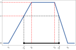
Figure 1: A trapezoidal fuzzy number $\widetilde{r}=(r_{1},r_{2},r_{3},r_{4})$ and its $\alpha$-cut $[r^{1}_{\alpha},r^{2}_{\alpha}]$ for some $\alpha$ between 0 and 1.

It is clear that the $\alpha$-cuts as above for $0\leq\alpha\leq 1$ determine the fuzzy number $\widetilde{r}$. Therefore one can identify any fuzzy number $\widetilde{r}\in\mathcal{F}(\mathbb{R})$ with its $\alpha$-cuts and write

$$\widetilde{r}=\{(r^{1}_{\alpha},r^{2}_{\alpha}):0\leq\alpha\leq 1\}.$$

Now, given two fuzzy numbers $\widetilde{r}=\{(r^{1}_{\alpha},r^{2}_{\alpha}):0\leq\alpha\leq 1\}$ and $\widetilde{s}=\{(s^{1}_{\alpha},s^{2}_{\alpha}):0\leq\alpha\leq 1\}$ in $\mathcal{F}(\mathbb{R})$, one can define their some $\widetilde{r}+\widetilde{s}$ and product $\widetilde{r}\,\widetilde{s}$ to be the unique fuzzy numbers whose representations in terms of $\alpha$-cuts are given by

$$\widetilde{r}+\widetilde{s}=\{(r^{1}_{\alpha}+s^{1}_{\alpha},r^{2}_{\alpha}+s^{2}_{\alpha}):0\leq\alpha\leq 1\},$$

and

$$\widetilde{r}\,\widetilde{s}=\{\left(\min(r^{1}_{\alpha}s^{1}_{\alpha},r^{1}_{\alpha}s^{2}_{\alpha},r^{2}_{\alpha}s^{1}_{\alpha},r^{2}_{\alpha}s^{2}_{\alpha}),\max(r^{1}_{\alpha}s^{1}_{\alpha},r^{1}_{\alpha}s^{2}_{\alpha},r^{2}_{\alpha}s^{1}_{\alpha},r^{2}_{\alpha}s^{2}_{\alpha})\right):0\leq\alpha\leq 1\}.$$

We note that $\widetilde{r}\,\widetilde{s}$ $=$ $\{(r^{1}_{\alpha}s^{1}_{\alpha},r^{2}_{\alpha}s^{2}_{\alpha}):0\leq\alpha\leq 1\},$ if $r^{1}_{\alpha},s^{1}_{\alpha}\geq 0$. Without using the $\alpha$-cuts, the above operations are written in terms of the following more complicated formulas:

$$(\widetilde{r}+\widetilde{s})(z)=\sup_{x+y=z}\min(\widetilde{r}(x),\widetilde{s}(y)),\quad(\widetilde{r}\,\widetilde{s})(z)=\sup_{xy=z}\min(\widetilde{r}(x),\widetilde{s}(y)).$$

Another important tool that we need is the extension principle which allows one to extend the domain of a function defined on real numbers to fuzzy numbers. That is, given a function $h:\mathbb{R}\to\mathbb{R}$ and a fuzzy number $\widetilde{r}$ one defines $\widetilde{s}=h(\widetilde{r})\in\mathcal{F}(\mathbb{R})$ by:

$$\widetilde{s}(z)=h(\widetilde{r})(z)=\sup_{h(x)=z}\widetilde{r}(x).$$

In practice, one can conveniently work with the $\alpha$-cuts of $\widetilde{s}=h(\widetilde{r})$ which allow one to write:

$$\widetilde{s}=h(\widetilde{r})=\left\{(s^{1}_{\alpha},s^{2}_{\alpha}):0\leq\alpha\leq 1\right\},$$ (10)

where

$$s^{1}_{\alpha}=\min_{x\in[r^{1}_{\alpha},r^{2}_{\alpha}]}h(x),\qquad s^{2}_{\alpha}=\max_{x\in[r^{1}_{\alpha},r^{2}_{\alpha}]}h(x).$$ (11)

3.2 Fuzzy random variables and their expectations as fuzzy numbers

We now discuss the notion of a fuzzy random variable $\widetilde{X}$. Recall that a random variable $X$ on a probability space $(\Omega,\mathcal{M},P)$, where $\mathcal{M}$ is its $\sigma$-algebra of events, is a measurable map $X:\Omega\to\mathbb{R}$ and its expectation is defined to be $\mathbb{E}[X]=\int_{\Omega}X(\omega)\,dP(\omega)$. The random variable $X$ induces a probability measure $\mu_{X}$ on $\mathbb{R}$ defined by $\mu_{X}([a,b])$$=$ $P(X\in[a,b])$$=$$P(X^{-1}([a,b]))$ for any interval $[a,b]\subset\mathbb{R}$. If $\mu_{X}$ is absolutely continuous with respect to the Lebesgue measure, one can write $d\mu_{X}(x)=f(x)\,dx$, where $f_{X}(x)$ is called the probability density function of $X$. Therefore $P(X\in[a,b])=\int_{a}^{b}f_{X}(x)\,dx$, and it then follows that $\mathbb{E}[X]=\int_{-\infty}^{\infty}xf_{X}(x)\,dx$ and more generally $\mathbb{E}[h(X)]=\int_{-\infty}^{\infty}h(x)f_{X}(x)\,dx$.

A fundamental fact here is that for any interval $[a,b]\subset\mathbb{R}$, and any ordinary random variable $X$ as above, the probability $P(X\in[a,b])$ is a certain real number. However, there are situations in which there is no such certainty, and one wishes to consider a range of valued possibilities for $P(X\in[a,b])$, where the notion of a fuzzy number is useful. That is, one can define a fuzzy random variable $\widetilde{X}$ on a probability space $(\Omega,\mathcal{M},P)$ to be a map from $\Omega$ to the set of fuzzy numbers $\mathcal{F}(\mathbb{R})$, denoted in the $\alpha$-cuts notation by $\widetilde{X}(\omega)=\{(X^{1}_{\alpha}(\omega),X^{2}_{\alpha}(\omega)):0\leq\alpha\leq 1\}$, such that the functions $X^{1}_{\alpha},X^{2}_{\alpha}:\Omega\to\mathbb{R}$ are measurable, and the probability of $\widetilde{X}$ belonging to an interval $[a,b]\subset\mathbb{R}$ is a fuzzy number given by $\alpha$-cuts as:

$$\widetilde{P}(\widetilde{X}\in[a,b])=\Big{\{}\left(\int_{a}^{b}f^{1}_{\alpha}(x)\,dx,\int_{a}^{b}f^{2}_{\alpha}(x)\,dx\right):0\leq\alpha\leq 1\Big{\}},$$

for suitable probability distribution functions $f^{1}_{\alpha}$ and $f^{2}_{\alpha}$. Therefore, the expectation $\widetilde{\mathbb{E}}[\widetilde{X}]=\{(\mathbb{E}[X^{1}_{\alpha}],\mathbb{E}[X^{2}_{\alpha}]):0\leq\alpha\leq 1\}$ is also a fuzzy number, which can be calculated by writing

$$\widetilde{\mathbb{E}}[\widetilde{X}]=\Big{\{}\left(\int_{-\infty}^{\infty}xf^{1}_{\alpha}(x)\,dx,\int_{-\infty}^{\infty}xf^{2}_{\alpha}(x)\,dx\right):0\leq\alpha\leq 1\Big{\}}.$$

4 The newsvendor optimization in fuzzy Gaussian mixture model

In the modeling of the distribution of the demand in the newsvendor problem, considering the technological advancements in recent years, there are two main types of data that are important to be considered, namely the online reviews and the historical data. Therefore, we wish to consider a Gaussian mixture model for the distribution of the demand of the form

$$X\sim pf_{1}(x)+(1-p)f_{2}(x),$$

where $0\leq p\leq 1$, and for each $i=1,2$, the function $f_{i}(x)$ is the probability density function of the normal distribution with mean $\mu_{i}$ and standard deviation $\sigma_{i}$, namely:

$$f_{i}(x)=(2\pi\sigma_{i}^{2})^{-1/2}\exp\left(-(x-\mu_{i})^{2}/(2\sigma_{i}^{2})\right),\quad i=1,2.$$ (12)

We note that we shall denote by $F_{i}$ the cumulative distribution functions corresponding to each $f_{i}$. The $\mu_{i}$ and $\sigma_{i}$ are determined respectively for $i=1,2$ by considering the online reviews and the historical data. Since one has access to large amounts of each of these data types, it is natural to consider them to have normal distributions and to derive values for the $\mu_{i}$ and $\sigma_{i}$ from the available data. However, there is considerable uncertainty in choosing the weight $p$ appropriately since one does not know how the two types of information come together to form the forthcoming demand $X$. Therefore in this article we use fuzzy numbers to analyze models that incorporate the uncertainties surrounding the weight $p$.

4.1 Gaussian mixture model with $p=E[\widetilde{p}]$ for the demand $X$

In this model, we use the online reviews and the historical data (along with information such as the availability of the reviews to potential merchants, their social habits, decision making behavior, etc.) to find a trapezoidal fuzzy number $\widetilde{p}=(p_{1},p_{2},p_{3},p_{4})$ (with $0\leq p_{1}\leq p_{2}\leq p_{3}\leq p_{4}\leq 1$) that incorporates uncertainties regarding how the two data types weigh in the formation of the demand $X$. We then consider the probability distribution function of the demand $X$ to be of the form

$$f_{X}(x)=E[\widetilde{p}]f_{1}(x)+(1-E[\widetilde{p}])f_{2}(x),$$ (13)

where $E[\widetilde{p}]=(p_{1}+p_{2}+p_{3}+p_{4})/4$ is the expected value of $\widetilde{p}$ introduced by (9), and, for each $i=1,2$, $f_{i}$ is as in (12).

In this case, one can use the classical solution of the newsvendor problem as discussed in §2 to find the optimal order quantity. That is, one can use (5) to optimize the expectation of the profit by ordering the quantity

$$Q_{\widetilde{p}}^{*}=F_{X}^{-1}\left(\frac{M-C}{M-V}\right),$$ (14)

where the role of the fuzzy number $\widetilde{p}$ is that its expected value $E[\widetilde{p}]$ appears in $F_{X}(x)=\int_{-\infty}^{x}\left(E[\widetilde{p}]f_{1}(t)+(1-E[\widetilde{p}])f_{2}(t)\right)\,dt$ $=$ $E[\widetilde{p}]F_{1}(x)+(1-E[\widetilde{p}])F_{2}(x)$.

4.2 Gaussian mixture model for $X$ with $p_{m}\leq p\leq p_{M}$ and optimization

We now consider the case when one wishes to consider the demand $X$ to have a Gaussian mixture distribution where the weigh $p$ is uniformly distributed in a subinterval $[p_{m},p_{M}]$ of the interval $[0,1]$. Therefore, one has

$$f_{X}(x)=pf_{1}(x)+(1-p)f_{2}(x),$$ (15)

with $f_{i}$ for $i=1,2$ as in (12), and the weight is a rectangular fuzzy number in the sense that it is a special trapezoidal fuzzy number of the form $(p_{m},p_{m},p_{M},p_{M})$.

For this model, the expectation of the profit $\mathbb{E}[\pi(X)]$ is clearly a function of the weight $p$. Thus, we find the optimal order quantity $Q$ that maximizes the average defined by

$$\overline{\mathbb{E}}[\pi(X)]=\frac{1}{p_{M}-p_{m}}\int_{p_{m}}^{p_{M}}\mathbb{E}[\pi(X)](p)\,dp.$$ (16)

Using (3) and (15), we have

$$\mathbb{E}[\pi(X)](p) = p\left(\int_{-\infty}^{Q}(Ax+aQ)f_{1}(x)\,dx+\int_{Q}^{\infty}bQf_{1}(x)\,dx\right)$$

$$+ (1-p)\left(\int_{-\infty}^{Q}(Ax+aQ)f_{2}(x)\,dx+\int_{Q}^{\infty}bQf_{2}(x)\,dx\right).$$

The latter yields:

$$\overline{\mathbb{E}}[\pi(X)] = \frac{1}{p_{M}-p_{m}}\int_{p_{m}}^{p_{M}}\mathbb{E}[\pi(X)](p)\,dp$$

$$= \frac{1}{2}\left(p_{M}+p_{m}\right)\Big{(}\int_{-\infty}^{Q}Axf_{1}(x)\,dx+aQF_{1}(Q)+bQ\left(1-F_{1}(Q)\right)\Big{)}$$

$$+ \frac{1}{2}\left(2-p_{m}-p_{M}\right)\Big{(}\int_{-\infty}^{Q}Axf_{2}(x)\,dx+aQF_{2}(Q)+bQ\left(1-F_{2}(Q)\right)\Big{)}.$$

Now we can optimize the average $\overline{\mathbb{E}}[\pi]$ by directly calculating its first and second derivatives of $Q$. By direct calculation, and replacing $A,a,b$ with the values given in (2), we find that:

$$\frac{d}{dQ}\overline{\mathbb{E}}[\pi(X)]=$$

$$\frac{1}{2}\Big{(}\big{(}\left(p_{m}+p_{M}-2\right)F_{2}(Q)-\left(p_{m}+p_{M}\right)F_{1}(Q)\big{)}(M-V)-2(C-M)\Big{)}.$$

Therefore, the only solution of the equation $\frac{d}{dQ}\overline{\mathbb{E}}[\pi(X)]=0$ is the point

$$\overline{Q}_{[p_{m},p_{M}]}^{*}=\left(\left(\frac{p_{m}+p_{M}}{2}\right)F_{1}+\left(1-\frac{p_{m}+p_{M}}{2}\right)F_{2}\right)^{-1}\left(\frac{M-C}{M-V}\right).$$ (17)

We also find that the second derivative is given by

$$\frac{d^{2}}{dQ^{2}}\overline{\mathbb{E}}[\pi(X)]=\frac{1}{2}\left(\left(p_{m}+p_{M}\right)\left(f_{2}(Q)-f_{1}(Q)\right)-2f_{2}(Q)\right)(M-V).$$

It can now be seen that $\frac{d^{2}}{dQ^{2}}\overline{\mathbb{E}}[\pi(X)]<0$, thus $\overline{\mathbb{E}}[\pi(X)]$ is a concave function of $Q$. Because, we clearly have the natural condition $M-V>0$, and we write the other factor $\left(\left(p_{m}+p_{M}\right)\left(f_{2}(Q)-f_{1}(Q)\right)-2f_{2}(Q)\right)$ of $\frac{d^{2}}{dQ^{2}}\overline{\mathbb{E}}[\pi(X)]$ as the following to see that it is the sum of three negative terms:

$$(p_{m}-1)f_{2}(Q)-(p_{m}+p_{M})f_{1}(Q)+(p_{M}-1)f_{2}(Q)<0.$$

Therefore $\frac{d^{2}}{dQ^{2}}\overline{\mathbb{E}}[\pi(X)]<0$, and the optimal quantity $\overline{Q}_{[p_{m},p_{M}]}^{*}$ given by (17) uniquely maximizes the average profit expectation $\overline{\mathbb{E}}[\pi(X)]$ in this model given by (16).

We now easily observe a compatibility between the optimal quantities $Q_{\widetilde{p}}^{*}$ given by (14) for the model (13), and the optimal quantity $\overline{Q}_{[p_{m},p_{M}]}^{*}$ given by (17) for the model (15). That is, since $E[(p_{m},p_{m},p_{M},p_{M})]=(1/4)(2p_{m}+2p_{M})=(1/2)(p_{m}+p_{M})$, we have:

$$Q_{(p_{m},p_{m},p_{M},p_{M})}^{*}=\overline{Q}_{[p_{m},p_{M}]}^{*}.$$ (18)

4.3 Fuzzy Gaussian mixture model for $X$ and fuzzy optimization

We now consider a model for the demand to be a fuzzy random variable of Gaussian mixture type and will denote it $\widetilde{X}$. The significance of this model is that it can incorporate a general trapezoidal fuzzy number $\widetilde{p}$ as the weight of the online reviews that contribute to the formation of the demand. We then use the machinery of fuzzy calculus to calculate the the profit $\widetilde{Y}=\pi(\widetilde{X})$ as a fuzzy random variable whose expectation $\mathbb{E}(\widetilde{Y})$ will be a fuzzy number with non-linear sides: it will be more general than the trapezoidal case as the end points of its $\alpha$-cuts are given by quadratic expressions in $\alpha$. We shall then defuzzify $\mathbb{E}(\widetilde{Y})$ in a natural manner for our management purposes, and will present the optimal order quantity $Q$ that maximizes the defuzzified quantity.

Therefore, we consider the normal probability distributions $f_{1}$ and $f_{2}$ as in (12), which separately reflect the distribution of the demand based on the online reviews and historical sales. We then use the information such as the expert opinion, availability of the reviews to potential merchants, social habits of the merchants, decision making behavior, etc., to find a fuzzy number

$$\widetilde{p}=(p_{1},p_{2},p_{3},p_{4}),\quad 0\leq p_{1}\leq p_{2}\leq p_{3}\leq p_{4}\leq 1,$$

which reflects the weight of the online reviews in the formation of the demand and can incorporate the uncertainties in the weight. In our model, we choose the numbers $p_{1}$ and $p_{2}$ independently from the numbers $p_{3}$ and $p_{4}$ by using separate parts of the data so that the random variables $X^{1}_{\alpha}$ and $X^{2}_{\alpha}$ whose probability distributions are defined below are independent:

$$f_{X^{1}_{\alpha}}(x)=p_{1}^{\alpha}f_{1}(x)+(1-p_{1}^{\alpha})f_{2}(x),$$

$$f_{X^{2}_{\alpha}}(x)=p_{2}^{\alpha}f_{1}(x)+(1-p_{2}^{\alpha})f_{2}(x).$$

We now consider the demand to have the fuzzy random variable $\widetilde{X}$ defined in terms of its $\alpha$-cuts by

$$\widetilde{X}=\{(X^{(1)}_{\alpha},X^{(2)}_{\alpha}),0\leq\alpha\leq 1\},$$ (19)

where

$$X^{(1)}_{\alpha}=\min(X^{1}_{\alpha},X^{2}_{\alpha}),\quad X^{(2)}_{\alpha}=\max(X^{1}_{\alpha},X^{2}_{\alpha}).$$

Lemma 4.1.

The joint probability distribution function of the random variables $X^{(1)}_{\alpha}$ and $X^{(2)}_{\alpha}$, denoted by $f_{X^{(1,2)}_{\alpha}}$, is given by

$$f_{X^{(1,2)}_{\alpha}}(x_{1},x_{2})=\begin{cases}f_{X^{1}_{\alpha}}(x_{1})f_{X^{2}_{\alpha}}(x_{2})+f_{X^{2}_{\alpha}}(x_{1})f_{X^{1}_{\alpha}}(x_{2}),\quad x_{1}\leq x_{2},\\ 0,\quad x_{2}<x_{1}.\end{cases}$$

Proof.

From the definition of $X^{(1)}_{\alpha}$ and $X^{(2)}_{\alpha}$, we always have $X^{(1)}_{\alpha}\leq X^{(2)}_{\alpha}$ and therefore $f_{X^{(1,2)}_{\alpha}}(x_{1},x_{2})=0$ when $x_{2}<x_{1}$. In order to calculate $f_{X^{(1,2)}_{\alpha}}(x_{1},x_{2})$ when $x_{1}\leq x_{2}$, we calculate

$$F_{X^{(1,2)}_{\alpha}}(x_{1},x_{2}) = P\left(X^{(1)}_{\alpha}\leq x_{1},X^{(2)}_{\alpha}\leq x_{2}\right)$$

$$= P\left(X^{1}_{\alpha}\leq x_{1},X^{2}_{\alpha}\leq x_{1}\right)+P\left(X^{1}_{\alpha}\leq x_{1},x_{1}<X^{2}_{\alpha}\leq x_{2}\right)$$

$$+ P\left(X^{2}_{\alpha}\leq x_{1},x_{1}<X^{1}_{\alpha}\leq x_{2}\right)$$

$$= F_{X^{1}_{\alpha}}(x_{1})F_{X^{2}_{\alpha}}(x_{1})+F_{X^{1}_{\alpha}}(x_{1})\left(F_{X^{2}_{\alpha}}(x_{2})-F_{X^{2}_{\alpha}}(x_{1})\right)$$

$$+ F_{X^{2}_{\alpha}}(x_{1})\left(F_{X^{1}_{\alpha}}(x_{2})-F_{X^{1}_{\alpha}}(x_{1})\right),$$

which yields:

$$f_{X^{(1,2)}_{\alpha}}(x_{1},x_{2})=\frac{\partial^{2}F_{X^{(1,2)}_{\alpha}}}{\partial x_{1}\partial x_{2}}(x_{1},x_{2})=f_{X^{1}_{\alpha}}(x_{1})f_{X^{2}_{\alpha}}(x_{2})+f_{X^{2}_{\alpha}}(x_{1})f_{X^{1}_{\alpha}}(x_{2}).$$

∎

We need the following statement for defuzzifications in the sequel, which involve integrations over $\alpha$ from 0 to 1.

Lemma 4.2.

When $x_{1}\leq x_{2}$, we have

$$\int_{0}^{1}f_{X^{(1,2)}_{\alpha}}(x_{1},x_{2})\,d\alpha=$$

$$P_{1}\,f_{1}\left(x_{1}\right)f_{1}\left(x_{2}\right)+P_{2}\left(f_{1}\left(x_{1}\right)f_{2}\left(x_{2}\right)+f_{2}\left(x_{1}\right)f_{1}\left(x_{2}\right)\right)+P_{3}\,f_{2}\left(x_{1}\right)f_{2}\left(x_{2}\right),$$

where

$$P_{1} = \frac{p_{1}p_{3}}{3}+\frac{2p_{2}p_{3}}{3}+\frac{2p_{1}p_{4}}{3}+\frac{p_{2}p_{4}}{3},$$ (20)

$$P_{2} = \frac{p_{1}}{2}-\frac{p_{3}p_{1}}{3}-\frac{2p_{4}p_{1}}{3}+\frac{p_{2}}{2}+\frac{p_{3}}{2}+\frac{p_{4}}{2}-\frac{2p_{2}p_{3}}{3}-\frac{p_{2}p_{4}}{3},$$

$$P_{3} = \frac{p_{3}p_{1}}{3}+\frac{2p_{4}p_{1}}{3}-p_{1}-p_{2}+\frac{2p_{2}p_{3}}{3}-p_{3}+\frac{p_{2}p_{4}}{3}-p_{4}+2.$$

Proof.

Using Lemma 4.1 and direct substitutions, when $x_{1}\leq x_{2}$, we have:

$$f_{X^{(1,2)}_{\alpha}}(x_{1},x_{2})=$$

$2f_{1}\left(x_{1}\right)f_{1}\left(x_{2}\right)p^{1}_{\alpha}p^{2}_{\alpha}+f_{2}\left(x_{1}\right)f_{1}\left(x_{2}\right)p^{1}_{\alpha}-2f_{2}\left(x_{1}\right)f_{1}\left(x_{2}\right)p^{1}_{\alpha}p^{2}_{\alpha}+f_{2}\left(x_{1}\right)f_{1}\left(x_{2}\right)p^{2}_{\alpha}+f_{1}\left(x_{1}\right)f_{2}\left(x_{2}\right)p^{1}_{\alpha}-2f_{1}\left(x_{1}\right)f_{2}\left(x_{2}\right)p^{1}_{\alpha}p^{2}_{\alpha}+f_{1}\left(x_{1}\right)f_{2}\left(x_{2}\right)p^{2}_{\alpha}-2f_{2}\left(x_{1}\right)f_{2}\left(x_{2}\right)p^{1}_{\alpha}+2f_{2}\left(x_{1}\right)f_{2}\left(x_{2}\right)p^{1}_{\alpha}p^{2}_{\alpha}-2f_{2}\left(x_{1}\right)f_{2}\left(x_{2}\right)p^{2}_{\alpha}+2f_{2}\left(x_{1}\right)f_{2}\left(x_{2}\right).$

Then, we find the result by the substitution

$$p^{1}_{\alpha}=p_{1}+(p_{2}-p_{1})\alpha,\quad p^{2}_{\alpha}=p_{4}+(p_{3}-p_{4})\alpha,$$

and direct integration over $\alpha$ from 0 to 1. ∎

Also, for the optimizations in the following subsections, we shall need the following properties of $P_{1},P_{2},P_{3}$ given by (20).

Lemma 4.3.

We have:

$$0\leq P_{1},P_{3}\leq 2,\quad 0\leq P_{2}\leq 1,\quad\frac{1}{2}P_{1}+P_{2}+\frac{1}{2}P_{3}=1.$$

and

$$P_{1}+2P_{2}+P_{3}=2.$$

Proof.

Since $0\leq p_{1}\leq p_{2}\leq p_{3}\leq p_{4}\leq 1$, it is clear that $0\leq P_{1}\leq 2$. One can then see that by setting $q_{i}=1-p_{i}$ for $i=1,\dots,4$ one has

$$P_{3}=\frac{q_{1}q_{3}}{3}+\frac{2q_{2}q_{3}}{3}+\frac{2q_{1}q_{4}}{3}+\frac{q_{2}q_{4}}{3},$$

which shows that $0\leq P_{3}\leq 2$. The identity $P_{1}+2P_{2}+P_{3}=2$ can be checked directly, which yields:

$$P_{2}=1-\frac{1}{2}P_{1}-\frac{1}{2}P_{3}\leq 1.$$

In order to see that $P_{2}\geq 0$, we write

$$2P_{2} = p_{1}+p_{2}+p_{3}+p_{4}-\frac{2}{3}p_{3}p_{1}-\frac{4}{3}p_{4}p_{1}-\frac{4}{3}p_{2}p_{3}-\frac{2}{3}p_{2}p_{4}$$

$$\geq p_{1}^{2}+p_{2}^{2}+p_{3}^{2}+p_{4}^{2}-\frac{2}{3}p_{3}p_{1}-\frac{4}{3}p_{4}p_{1}-\frac{4}{3}p_{2}p_{3}-\frac{2}{3}p_{2}p_{4}$$

$$= \begin{pmatrix}p_{1}&p_{2}&p_{3}&p_{4}\\ \end{pmatrix}\left(\begin{array}[]{cccc}1&0&-1/3&-2/3\\ 0&1&-2/3&-1/3\\ -1/3&-2/3&1&0\\ -2/3&-1/3&0&1\\ \end{array}\right)\begin{pmatrix}p_{1}\\ p_{2}\\ p_{3}\\ p_{4}\end{pmatrix}.$$

The latter is non-negative since the above square matrix is symmetric and its eigenvalues are the non-negative numbers $2,4/3,2/3,0$.

∎

By using (10) and (11), we apply the profit function $\pi$ to the fuzzy random variable $\widetilde{X}$ and obtain the profit of the newsvendor as a fuzzy random variable $\widetilde{Y}=\pi(\widetilde{X})$:

$$\widetilde{X}=\left\{(X^{(1)}_{\alpha},X^{(2)}_{\alpha}):0\leq\alpha\leq 1\right\},\quad\widetilde{Y}=\pi(\widetilde{X})=\left\{(Y^{1}_{\alpha},Y^{2}_{\alpha}):0\leq\alpha\leq 1\right\},$$

where

$$Y^{1}_{\alpha}=h_{1}(X^{(1)}_{\alpha},X^{(2)}_{\alpha})=\begin{cases}AX^{(1)}_{\alpha}+aQ,\quad X^{(1)}_{\alpha}\leq X^{(2)}_{\alpha}\leq Q,\\ bQ,\quad Q\leq X^{(1)}_{\alpha}\leq X^{(2)}_{\alpha},\\ \min\Big{(}AX^{(1)}_{\alpha}+aQ,bQ\Big{)},\quad X^{(1)}_{\alpha}\leq Q\leq X^{(2)}_{\alpha},\end{cases}$$

$$Y^{2}_{\alpha}=h_{2}(X^{(1)}_{\alpha},X^{(2)}_{\alpha})=\begin{cases}AX^{(2)}_{\alpha}+aQ,\quad X^{(1)}_{\alpha}\leq X^{(2)}_{\alpha}\leq Q,\\ bQ,\quad Q\leq X^{(1)}_{\alpha}\leq X^{(2)}_{\alpha},\\ (A+a)Q=bQ,\quad X^{(1)}_{\alpha}\leq Q\leq X^{(2)}_{\alpha}.\end{cases}$$

4.3.1 Optimization of $\int_{0}^{1}\mathbb{E}[Y^{1}_{\alpha}]\,d\alpha$

We have:

$$\mathbb{E}[Y^{1}_{\alpha}] = \int_{-\infty}^{Q}dx_{1}\int_{x_{1}}^{Q}dx_{2}\,\left(Ax_{1}+aQ\right)f_{X^{(1,2)}_{\alpha}}(x_{1},x_{2})$$

$$+ \int_{Q}^{\infty}dx_{1}\int_{x_{1}}^{\infty}dx_{2}\,bQ\,f_{X^{(1,2)}_{\alpha}}(x_{1},x_{2})$$

$$+ \int_{-\infty}^{Q}dx_{1}\int_{Q}^{\infty}dx_{2}\,\left(Ax_{1}+aQ\right)f_{X^{(1,2)}_{\alpha}}(x_{1},x_{2}).$$

In order to find the quantity $Q$ that maximizes $\int_{0}^{1}\mathbb{E}[Y^{1}_{\alpha}]\,d\alpha$, we use Lemma 4.2 and calculate its first and second derivatives with respect to $Q$. We find that:

$$\frac{d}{dQ}\int_{0}^{1}\mathbb{E}[Y^{1}_{\alpha}]\,d\alpha = -C+M+\left(-2C+M+V\right)G(Q)$$

$$+ \left(C-V\right)H(Q)+\left(-M+V\right)J(Q),$$

where

$$G(x) = \int_{-\infty}^{x}g(t)\,dt,$$ (24)

$$g(t) = P_{1}\,f_{1}(t)F_{1}(t)+P_{2}\big{(}f_{1}(t)F_{2}(t)+f_{2}(t)F_{1}(t)\big{)}+P_{3}\,f_{2}(t)F_{2}(t),$$

$$H(x) = P_{1}\,F_{1}(x)^{2}+2P_{2}\,F_{1}(x)F_{2}(x)+P_{3}\,F_{2}(x)^{2},$$

$$J(x) = P_{1}\,F_{1}(x)+P_{2}\left(F_{1}(x)+F_{2}(x)\right)+P_{3}\,F_{2}(x).$$

We now make some observations about the functions $G,H,J$, which shall be insightful in the optimizations in the sequel.

Lemma 4.4.

The functions $G,H,J$ are non-negative, non-decreasing, for any real number $x$:

$$G(x)=\frac{1}{2}H(x),\quad H(x)\leq J(x),$$ (25)

and

$$\lim_{x\to-\infty}G(x)=\lim_{x\to-\infty}\frac{1}{2}H(x)=\lim_{x\to-\infty}\frac{1}{2}J(x)=0,$$

$$\lim_{x\to\infty}G(x)=\lim_{x\to\infty}\frac{1}{2}H(x)=\lim_{x\to\infty}\frac{1}{2}J(x)=1.$$

Proof.

It is clear that these functions are non-negative and non-decreasing. Using the definitions of the functions, we can write

$$G(x) = \int_{-\infty}^{x}\left(P_{1}\,f_{1}(t)F_{1}(t)+P_{2}\big{(}f_{1}(t)F_{2}(t)+f_{2}(t)F_{1}(t)\big{)}+P_{3}\,f_{2}(t)F_{2}(t)\right)dt$$

$$= \int_{-\infty}^{x}\frac{d}{dt}\left(\frac{P_{1}}{2}F_{1}(t)^{2}+P_{2}\,F_{1}(t)F_{2}(t)+\frac{P_{3}}{2}F_{2}(t)^{2}\right)dt$$

$$= \frac{P_{1}}{2}F_{1}(x)^{2}+P_{2}\,F_{1}(x)F_{2}(x)+\frac{P_{3}}{2}F_{2}(x)^{2}$$

$$= \frac{1}{2}H(x).$$

The fact that $H(x)\leq J(x)$ is an easy consequence of the fact that $0\leq F_{1}(x)\leq 1,$ $0\leq F_{2}(x)\leq 1$ and that $0\leq P_{1},P_{2},P_{3}$ (proved in Lemma 4.3). The vanishing of these functions in limit at $-\infty$ is also easily seen, and the limits at $\infty$ are calculated by considering the fact that $P_{1}/2+P_{2}+P_{3}/2=1$. ∎

We also have

$$\lim_{Q\to-\infty}\left(\frac{d}{dQ}\int_{0}^{1}\mathbb{E}[Y^{1}_{\alpha}]\,d\alpha\right)=-C+M>0,$$

$$\lim_{Q\to\infty}\left(\frac{d}{dQ}\int_{0}^{1}\mathbb{E}[Y^{1}_{\alpha}]\,d\alpha\right)=-C+V<0.$$

For the second derivative we find that:

$$\frac{d^{2}}{dQ^{2}}\int_{0}^{1}\mathbb{E}[Y^{1}_{\alpha}]\,d\alpha$$

$$= (V-M)\Big{(}f_{1}(Q)\left((P_{1}(1-F_{1}(Q))+P_{2}(1-F_{2}(Q))\right)\Big{)}$$

$$+ (V-M)\Big{(}f_{2}(Q)\left(P_{2}(1-F_{1}(Q))+P_{3}(1-F_{2}(Q))\right)\Big{)}<0,$$

which shows that we have a concave function of $Q$. Therefore, the unique optimal quantity $Q$ that maximizes $\int_{0}^{1}\mathbb{E}[Y^{1}_{\alpha}]\,d\alpha$ is the solution of setting (4.3.1) equal to 0. By defining the function

$$F_{\widetilde{p},L}(x)=\frac{2C-M-V}{M-V}G(x)+\frac{-C+V}{M-V}H(x)+J(x)=-\frac{1}{2}H(x)+J(x),$$ (27)

where the last identity follows from (25), this quantity is given by

$$Q^{*}_{\widetilde{p},L}=F^{-1}_{\widetilde{p},L}\left(\frac{M-C}{M-V}\right).$$ (28)

4.3.2 Optimization of $\int_{0}^{1}\mathbb{E}[Y^{2}_{\alpha}]\,d\alpha$

Similarly, we start by writing the following expression:

$$\mathbb{E}[Y^{2}_{\alpha}] = \int_{-\infty}^{\infty}dx_{1}\int_{x_{1}}^{\infty}dx_{2}\,h_{2}(x_{1},x_{2})\,f_{X^{(1,2)}_{\alpha}}(x_{1},x_{2})$$ (29)

$$= \int_{-\infty}^{Q}dx_{1}\int_{x_{1}}^{Q}dx_{2}\,\left(Ax_{2}+aQ\right)f_{X^{(1,2)}_{\alpha}}(x_{1},x_{2})$$

$$+ \int_{Q}^{\infty}dx_{1}\int_{x_{1}}^{\infty}dx_{2}bQf_{X^{(1,2)}_{\alpha}}(x_{1},x_{2})$$

$$+ \int_{-\infty}^{Q}dx_{1}\int_{Q}^{\infty}dx_{2}bQ\,f_{X^{(1,2)}_{\alpha}}(x_{1},x_{2}).$$

We then use Lemma 4.2, and calculate the derivatives of order one and two of $\int_{0}^{1}\mathbb{E}[Y^{2}_{\alpha}]\,d\alpha$ with respect to $Q$. We find that:

$$\frac{d}{dQ}\int_{0}^{1}\mathbb{E}[Y^{2}_{\alpha}]\,d\alpha = -C+M+(-2C+M+V)G(Q)$$

$$+ (C-M)H(Q)$$

where the functions $G,H,J$ are already given in (24). We also note that

$$\lim_{Q\to-\infty}\left(\frac{d}{dQ}\int_{0}^{1}\mathbb{E}[Y^{2}_{\alpha}]\,d\alpha\right)=-C+M>0,$$

$$\lim_{Q\to\infty}\left(\frac{d}{dQ}\int_{0}^{1}\mathbb{E}[Y^{2}_{\alpha}]\,d\alpha\right)=-C+V<0.$$

The function $\int_{0}^{1}\mathbb{E}[Y^{2}_{\alpha}]\,d\alpha$ is concave in $Q$ because its second derivative with respect to $Q$ is the sum of three negative terms:

$$\frac{d^{2}}{dQ^{2}}\int_{0}^{1}\mathbb{E}[Y^{2}_{\alpha}]\,d\alpha$$

$$= P_{1}f_{1}(Q)F_{1}(Q)(-M+V)$$

$$+ P_{2}\Big{(}f_{2}(Q)\big{(}F_{1}(Q)(-M+V)\big{)}+f_{1}(Q)\big{(}F_{2}(Q)(-M+V)\big{)}\Big{)}$$

$$+ P_{3}f_{2}(Q)F_{2}(Q)(-M+V)<0.$$

Therefore, the unique optimal solution that maximizes $\int_{0}^{1}\mathbb{E}[Y^{2}_{\alpha}]\,d\alpha$ is the quantity $Q$ that is the solution of setting (4.3.2) equal to 0. This is given by

$$Q^{*}_{\widetilde{p},R}=F^{-1}_{\widetilde{p},R}\left(\frac{M-C}{M-V}\right),$$ (32)

where considering (4.3.2) and (25):

$$F_{\widetilde{p},R}(x)=\frac{2C-M-V}{M-V}\,G(x)+\frac{M-C}{M-V}\,H(x)=\frac{1}{2}H(x).$$ (33)

4.3.3 Optimization of $(1-\beta)\int_{0}^{1}\mathbb{E}[Y^{1}_{\alpha}]\,d\alpha+\beta\int_{0}^{1}\mathbb{E}[Y^{2}_{\alpha}]\,d\alpha$

In the previous subsections, we have seen that when the demand $\widetilde{X}$ is a fuzzy random variable as introduced in (19), the expectation of the profit $\widetilde{Y}=\pi(\widetilde{X})$ is a fuzzy number whose $\alpha$-cuts are given by quadratic expressions in $\alpha$. By performing an integration over $\alpha$ and finding the optimal quantity $Q^{*}_{\widetilde{p},L}$ given by (28), we have introduced an optimal quantity that gives the largest possible average for the small possible values for the profit. Therefore, the quantity $Q^{*}_{\widetilde{p},L}$ can be used when the newsvendor wishes to go with minimum risk by choosing the order quantity that gives the security that the average of the small possible values of the fuzzy profit expectation is maximized. In the other direction, the optimal quantity $Q^{*}_{\widetilde{p},R}$ given by (32) maximizes the average over the greatest possible values for the fuzzy profit expectation. Therefore, the quantity $Q^{*}_{\widetilde{p},R}$ can be used if the newsvendor wishes to create maxim possibility for the profit at the price of being in the riskiest possible situation.

Thus, it is natural at this stage to use a real number $\beta$ in the interval $[0,1]$ as a risk factor so that the newsvendor can choose an optimal order quantity depending on the risk that they can afford. That is, we wish to find an optimal quantity $Q^{*}_{\widetilde{p},\beta}$ that maximizes

$$(1-\beta)\int_{0}^{1}\mathbb{E}[Y^{1}_{\alpha}]\,d\alpha+\beta\int_{0}^{1}\mathbb{E}[Y^{2}_{\alpha}]\,d\alpha.$$ (34)

Note that the latter defines a defuzzification that generalizes the one discussed in Remark 3.1.

Considering the calculations performed for the results in the previous subsections, we can find this optimal quantity quite easily. The reason is that, using (4.3.1) and (4.3.2), we have an explicit expression for the derivative of (34) with respect to $Q$. Since, using the information in (4.3.1) and (4.3.2), we have a concave expression, the unique optimal quantity that maximizes the defuzzified expectation of the fuzzy profit, given by (34), is the quantity

$$Q^{*}_{\widetilde{p},\beta}=F^{-1}_{\widetilde{p},\beta}\left(\frac{M-C}{M-V}\right),$$ (35)

where

$$F_{\widetilde{p},\beta}(x) = (1-\beta)F_{\widetilde{p},L}(x)+\beta F_{\widetilde{p},R}(x)$$

$$= \frac{2\beta-1}{2}H(x)+(1-\beta)J(x)$$

$$= \frac{1}{2}H(x)+(1-\beta)\left(J(x)-H(x)\right).$$

Clearly, the optimal solutions for $\beta=0$ and $\beta=1$ match with the solutions given by (28) and (32), respectively.

The resemblance between the formulas for the optimal solution (35) and the classical newsvendor solution (5) raises the question whether the function $F_{\widetilde{p},\beta}$ given by (4.3.3) is the cumulative distribution functions of a random variable. The following proposition in fact shows that one can take this point of view.

Proposition 4.1.

The function $F_{\widetilde{p},\beta}$, for any $\beta$ in the interval $[0,1]$, satisfies the properties of the cumulative distribution function of a random variable: it is non-negative, non-decreasing, tends to 0 at $-\infty$, and tends to 1 at $\infty$.

Proof.

This is a direct consequence of Lemma 4.4, (4.3.1), (4.3.2), and the fact that $F_{\widetilde{p},\beta}(x)=$ $(1-\beta)F_{\widetilde{p},L}(x)+\beta F_{\widetilde{p},R}(x)$. ∎

We now make an observation, which is in complete agreement with intuition:

Proposition 4.2.

The optimal order quantity $Q^{*}_{\widetilde{p},\beta}$ given by (35) is a non-decreasing function of the risk factor $\beta$.

Proof.

Using the fact $H(x)\leq J(x)$ from Lemma 4.4, it follows from the formula

$$F_{\widetilde{p},\beta}(x)=\frac{1}{2}H(x)+(1-\beta)\left(J(x)-H(x)\right)$$

that for any real number $x$, the value $F_{\widetilde{p},\beta}(x)$ defines a non-increasing function of the risk factor $\beta$. Therefore, $Q^{*}_{\widetilde{p},\beta}=F^{-1}_{\widetilde{p},\beta}\left(\frac{M-C}{M-V}\right)$ is non-decreasing in $\beta$. ∎

The fact that $Q^{*}_{\widetilde{p},\beta}$ is non-decreasing in $\beta$ justifies the reason for calling the latter the risk factor. Because when the newsvendor thinks of two order quantities $Q_{1}$ and $Q_{2}$ such that $Q_{1}<Q_{2}$, the profit function $\pi_{2}$ corresponding to $Q_{2}$ provides a wider range of possibilities for the gain and loss compared to the profit function $\pi_{1}$ corresponding to $Q_{1}$, as it can be seen in Figure 2. That is, if the newsvendor chooses the more risky case of ordering the larger quantity $Q_{2}$, then $\pi_{2}(x)>\pi_{1}(x)$ if and only if the demand $x$ is greater than

$$Q_{12}=\frac{M-C}{M-V}Q_{1}+\frac{C-V}{M-V}Q_{2}.$$

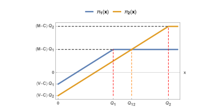
Figure 2: The profit function $\pi_{i}$ corresponds to the order quantity $Q_{i}$ for $i=1,2$.

Thus, the calculation of the probability that the demand is greater than $Q_{12}$ can help the newsvendor to choose between $Q_{1}$ and $Q_{2}$.

4.4 Newsvendoric defuzzifications of the fuzzy demand

Proposition 4.1 confirms that the function $F_{\widetilde{p},\beta}$ given by (4.3.3) defines the cumulative distribution function of a random variable, which will be denoted by $X_{\widetilde{p},\beta}$ hereafter. Hence, given the fuzzy random variable $\widetilde{X}$ defined in (19), considering (5), the optimal quantity given by (35) is the solution of the classical newsvendor problem when the demand is assumed to be the ordinary random variable $X_{\widetilde{p},\beta}$, whose distribution density function is:

$$f_{X_{\widetilde{p},\beta}}(x) = \frac{d}{dx}F_{\widetilde{p},\beta}(x)$$

$$= \frac{d}{dx}\left(\frac{2\beta-1}{2}H(x)+(1-\beta)J(x)\right)$$

$$= (2\beta-1)\big{(}f_{1}(x)\left(P_{1}F_{1}(x)+P_{2}F_{2}(x)\right)+f_{2}(x)\left(P_{2}F_{1}(x)+P_{3}F_{2}(x)\right)\big{)}$$

$$+ (\beta-1)\left(-\left(P_{1}+P_{2}\right)f_{1}(x)-\left(P_{2}+P_{3}\right)f_{2}(x)\right).$$

This means that, one can replace the demand $\widetilde{X}$, which is a fuzzy random variable, with an ordinary random variable, and consider the solution of the classical newsvendor problem to obtain the optimal quantity (35). Hence, we have arrived at a natural defuzzification of the fuzzy random variable $\widetilde{X}$ via our fuzzy newsvendor optimization.

We made the observation (18) to show that there is a relation between the optimizing quantities for the models written in §4.1 and §4.2. We now make observations in the following remark to show that the optimized quantity (35) and the distribution function given by (4.4) of the defuzzified random variable $\widetilde{X}_{\widetilde{p},\beta}$ relate to the optimized quantities (14) and (17) when $\beta=1/2$.

First, we explain how the intuitive model of §4.1 can be viewed as a particular case of the fuzzy model.

Remark 4.1.

Starting with a trapezoidal fuzzy number $\widetilde{p}=(p_{1},p_{2},p_{3},p_{4})$ and the fuzzy demand $\widetilde{X}$ as in (19), if one sets the risk factor $\beta$ equal to $1/2$, then the density of the corresponding defuzzified demand $X_{\widetilde{p},\frac{1}{2}}$ simplifies to

$$f_{X_{\widetilde{p},\frac{1}{2}}}(x)=pf_{1}(x)+(1-p)f_{2}(x),$$ (38)

where

$$p=\frac{P_{1}+P_{2}}{2}=\frac{1}{4}\left(p_{1}+p_{2}+p_{3}+p_{4}\right)=E[\widetilde{p}].$$

Therefore, the model written in §4.1, which was written intuitively, can be obtained as a special defuzzification of the fuzzy model treated in this subsection by setting $\beta=1/2$.

Now we explain that the second model with a rectangular fuzzy number, written in §4.2, can also be realized as a special case of the fuzzy model.

Remark 4.2.

If we assume that the fuzzy number $\widetilde{p}$ in the fuzzy demand model $\widetilde{X}$ given by (19) is rectangular as in the model in §4.2, namely $\widetilde{p}=$ $(p_{m},p_{m},p_{M},p_{M})$, then we have $P_{1}=2p_{m}p_{M}$, $P_{2}$ $=$ $-2p_{m}p_{M}+p_{m}+p_{M}$, and $P_{3}$ $=$ $2\left(1-p_{m}\right)\left(1-p_{M}\right)$. Therefore, for the particular risk factor $\beta=1/2$, the distribution of the defuzzification $X_{\widetilde{p},\frac{1}{2}}$ of $\widetilde{X}$ is given by

$$f_{X_{\widetilde{p},\frac{1}{2}}}(x)=pf_{1}(x)+(1-p)f_{2}(x),$$

where

$$p=\frac{P_{1}+P_{2}}{2}=\frac{p_{m}+p_{M}}{2}=E[\widetilde{p}].$$

Hence, the optimization in the second model written in §4.2 is also obtained as a special defuzzification of the fuzzy model by setting $\beta=1/2$.

Using the above remarks, we can now explain how the three models in this article associated with the fuzzy weight $\widetilde{p}$ reduce to the classical newsvendor model if there is no uncertainty in the choice of $\widetilde{p}$. In fact, this happens when the risk factor $\beta=1/2$ and the weight $\widetilde{p}$ is taken to be an ordinary (or a crisp) number.

Remark 4.3.

If the fuzzy number $\widetilde{p}$ in the fuzzy demand model $\widetilde{X}$ given by (19) is taken to be of the form $\widetilde{p}=(p,p,p,p)$, where $p$ is in the interval $[0,1]$, then $P_{1}=2p^{2}$, $P_{2}=-2(p-1)p$, $P_{3}=2(p-1)^{2}$, which yields $(P_{1}+P_{2})/2=p$ and $(P_{2}+P_{3})/2=1-p$. Then, if one takes the risk factor $\beta$ equal to $1/2$, considering Remarks 4.1 and 4.2, the three fuzzy models considered in this article reduce to the classical newsvendor problem with the distribution function of the demand given by $f_{X}(x)=$ $pf_{1}(x)+(1-p)f_{2}(x)$.

Following the above remarks, only when we have $\beta=1/2$ for the risk factor, the results that we have obtained by using the machinery of fuzzy random variables can be realized by the classical newsvendor analysis where the distribution function of the demand $X$ is of the form $pf_{1}(x)+(1-p)f_{2}(x)$.

Hence, a crucial result of our fuzzy analysis is the derivation of the distribution function $f_{X_{\widetilde{p},\beta}}$ given by (4.4) of the defuzzification $X_{\widetilde{p},\beta}$ of the fuzzy demand $\widetilde{X}$. That is, in order to incorporate the uncertainties related to the weight of the online reviews in the formation of the demand, for a general risk factor $\beta$ in the interval $[0,1]$, one can say that the optimal order quantity $Q^{*}_{\widetilde{p},\beta}$ is the solution of the newsvendor problem when the probability distribution function of the demand is taken to be the function $f_{X_{\widetilde{p},\beta}}$. Apparently, this function is by far more general than the distribution functions of the form $pf_{1}(x)+(1-p)f_{2}(x)$ that have been used classically and in the models written in §4.1 and §4.2. A great advantage of using the function $f_{X_{\widetilde{p},\beta}}$ is that it allows the newsvendor to use in the model the risk factor $\beta$ and the parameters of the fuzzy number $\widetilde{p}$ that incorporates the range of online reviews and their weight in the formation of the demand. The point is that, as indicated by (38), only when $\beta=1/2$, the function $f_{X_{\widetilde{p},\beta}}$ is realized by the classical form $pf_{1}(x)+(1-p)f_{2}(x)$. Therefore, the nontrivial generalization $f_{X_{\widetilde{p},\beta}}$ that we have obtained by means of the fuzzy machinery is more powerful for the purpose of capturing the distribution of the demand. We shall provide in the sequel identification strategies for the risk factor $\beta$ and the parameters of $\widetilde{p}$.

4.5 Risk-averse, risk-neutral, and risk-seeking decision making using the risk factor $\beta$

Our objective in this subsection is to show that in our approach, in a natural way, we have introduced an objective function in which the parameter $\beta$ can encode the risk attitude of the decision maker. More importantly, for any chosen risk factor, we have an analytic formula for the optimizing order quantity. It is in fact crucial to incorporate risk attitude in studies related to the newsvendor problem, since it is often essential for decision makers to have a control on their vulnerabilities to uncertainties. For studies in which mean-variance analysis is employed for the incorporation of risk attitude, we refer the reader to Choi et al. (2008), Wu et al. (2009), and references therein.

In our approach, we have introduced a novel objective function introduced in §4.3.3, namely

$$(1-\beta)\int_{0}^{1}\mathbb{E}[Y^{1}_{\alpha}]\,d\alpha+\beta\int_{0}^{1}\mathbb{E}[Y^{2}_{\alpha}]\,d\alpha,$$

which incorporates a risk factor $\beta$, and we have found analytically an order quantity $Q^{*}_{\widetilde{p},\beta}$ that optimizes our objective function for any given $\beta$. The following result shows that, using our model, the decision maker can increase its profit expectation by increasing the risk factor $\beta$.

Proposition 4.3.

The profit expectation $\mathbb{E}[\pi(X_{\widetilde{p},\beta})]$ evaluated at the optimal value $Q^{*}_{\widetilde{p},\beta}$ introduces an increasing function of the risk factor $\beta$.

Proof.

Using (6), we can write:

$$\mathbb{E}[\pi(X_{\widetilde{p},\beta})](Q^{*}_{\widetilde{p},\beta})=(-M+V)\int_{0}^{Q^{*}_{\widetilde{p},\beta}}F_{X_{\widetilde{p},\beta}}(t)\,dt+(M-C)Q^{*}_{\widetilde{p},\beta}.$$

We find that

$$\frac{d}{d\beta}\left(\mathbb{E}[\pi(X_{\widetilde{p},\beta})](Q^{*}_{\widetilde{p},\beta})\right)$$

$$= (V-M)\left(\int_{0}^{Q^{*}_{\widetilde{p},\beta}}\frac{\partial}{\partial\beta}F_{X_{\widetilde{p},\beta}}(t)\,dt+\left(\frac{d}{d\beta}Q^{*}_{\widetilde{p},\beta}\right)F_{X_{\widetilde{p},\beta}}(Q^{*}_{\widetilde{p},\beta})\right)$$

$$+ (M-C)\frac{d}{d\beta}Q^{*}_{\widetilde{p},\beta}$$

$$= (V-M)\left(\int_{0}^{Q^{*}_{\widetilde{p},\beta}}\frac{\partial}{\partial\beta}F_{X_{\widetilde{p},\beta}}(t)\,dt\right)$$

$$= (M-V)\left(\int_{0}^{Q^{*}_{\widetilde{p},\beta}}\left(J(t)-H(t)\right)\,dt\right),$$

where we use the fact that $F_{X_{\widetilde{p},\beta}}(Q^{*}_{\widetilde{p},\beta})=(M-C)/(M-V)$. Since $M-V>0$, and we know from Lemma 4.4 that $H(t)\leq J(t)$ for all $t$, we can conclude that $\mathbb{E}[\pi(X_{\widetilde{p},\beta})](Q^{*}_{\widetilde{p},\beta})$ is an increasing function of the risk factor $\beta$. ∎

Based on Remark 4.1, when $\beta=1/2$, our fuzzy model is equivalent to a risk-neutral classical newsvendor problem. Hence, based on the results presented in Propositions 4.2 and 4.3, a decision maker can use our fuzzy model as follows. In the risk-averse case, one can choose to have $0\leq\beta<1/2$, in the risk-neutral case $\beta=1/2$, and for risk-seeking $1/2<\beta\leq 1$.

Example 4.1.

In the most risk-seeking case, the decision maker chooses $\beta=1$, and models the distribution of the demand with

$$f_{X_{\widetilde{p},1}}(x)=P_{1}F_{1}(x)f_{1}(x)+P_{3}F_{2}(x)f_{2}(x)+P_{2}\left(F_{2}(x)f_{1}(x)+F_{1}(x)f_{2}(x)\right).$$

In this case, the order quantity is set by

$$Q^{*}_{\widetilde{p},1}=F^{-1}_{\widetilde{p},1}\left(\frac{M-C}{M-V}\right),$$ (39)

where

$$F_{\widetilde{p},1}(x)=\frac{1}{2}\left(P_{1}F_{1}(x){}^{2}+2P_{2}F_{1}(x)F_{2}(x)+P_{3}F_{2}(x){}^{2}\right).$$

5 Example of application of the fuzzy GMM

The aim of this section is twofold:

• To provide a concrete application scenario on how inventory managers could use both subjective and probabilistic measure of the demand uncertainty.

• To illustrate the implications of the mixture between the quantitative and subjective uncertainty of demand on inventory performance and to provide insights on the parameter inputs.

The source code of our simulations is available on GitHub.

5.1 Rationals for a fuzzy model

We present a heuristics and an experimental study to legitimate the use of fuzzy numbers in our models, and give recommendations on how to derive them experimentally.

In Section 4, we modelled the weight between online reviews and historical data in the formation of demand by a fuzzy number $\widetilde{p}=(p_{1},p_{2},p_{3},p_{4})$. We explain here how to derive $\widetilde{p}$ from online data.

Consider a vendor’s website, presenting its products for order and its customers online ratings for each of them, say on a 0 to 5 stars scale. Consider a given product presented online, and let $\bar{m}$ denote its average online ratings as displayed on its page.

We make the assumption that a proxy for the vendors’ clients are website visitors. We split visitors into “customers” (on records for previous purchases), and “prospects” (with no prior purchases).

The heuristics behind the following recommendation is the following:

• The left leg of $\widetilde{p}$, ($p_{1}$, $p_{2}$), is related to the minimum weight for reviews vs historical distributions. This concerns customers, who are less sensitive to reviews and more driven by their experience with past products they bought and might need to order regularly.

• The right leg of $\widetilde{p}$, ($p_{3}$,$p_{4}$), is related to the maximum weight for reviews vs historical distributions. This concerns prospects, who are sensitive to reviews since they have no experience with the company’s products.

We further split customers into: review insensitive (ri) costumers who visit the website to order a product they know/need, and review sensitive (rs) costumers who might change their order based on reviews they see. Let us denote by $n^{v}$ the total number of visitors on that page, $n^{c}$ the number of customers, and $n^{p}$ the number of prospects. We have $n^{v}=n^{c}+n^{p}=n^{ric}+n^{rsc}+n^{p}$, where $n^{ric}$ (resp. $n^{rsc}$) is the number of ri-customers (resp. rs-costumers).

The buying inclination of an rs-customer or a prospect checking up the product on that page is modelled with a trapezoidal fuzzy number $\widetilde{q}=(q_{1},q_{2},q_{3},q_{4})$, with integers $0\leq q_{1}\leq q_{2}\leq q_{3}=q_{4}=5$ as follows:

• The visitor is certain not to place an order if $\bar{m}\leq q_{1}$.

• The visitor is uncertain if $q_{1}<\bar{m}<q_{2}$.

• The visitor is certain to place an order if $\bar{m}\geq q_{2}$.

For $rs$-customers the associated fuzzy numbers are denoted $\widetilde{q}^{rsc}_{i}=(q_{i1}^{rsc},q_{i2}^{rsc},5,5)$, $i=1,\dots,n^{rsc}$, and for prospects $\widetilde{q}^{p}_{i}=(q_{i1}^{p},q_{i2}^{p},5,5)$, $i=1,\dots,n^{p}$. We assume that the expectations of prospects are higher than those of rsc-customers, that they need extra incentive to place an order. It follows that we model the $q_{ij}^{rsc}$ and $q_{ij}^{p}$ by Gaussian independent random variables with means satisfying

$$0\leq\mathbb{E}(q_{.1}^{rsc})<\mathbb{E}(q_{.2}^{rsc})<\mathbb{E}(q_{.1}^{p})<\mathbb{E}(q_{.2}^{p})\leq 5\,,$$

and the same variances.

We further split the $n^{rsc}=n^{rsc}_{0}+n^{rsc}_{1}+n^{rsc}_{2}$ $rs$-customers into $n^{rsc}_{0}$ who did not place an order, $n^{rsc}_{1}$ who ordered without hesitation (i.e. for which $q_{i2}^{rsc}\leq\bar{m}$), and $n^{rsc}_{2}$ who hesitated before ordering (i.e. for which $q_{i1}^{rsc}\leq\bar{m}<q_{i2}^{rsc}$). Also, we similarly split the $n^{p}=n^{p}_{0}+n^{p}_{1}+n^{p}_{2}$ prospects into $n^{p}_{0}$ who did not order, $n^{p}_{1}$ who ordered without hesitation (i.e. for which $q_{i2}^{p}\leq\bar{m}$), and $n^{p}_{2}$ who hesitated before ordering (i.e. for which $q_{i1}^{p}\leq\bar{m}<q_{i2}^{p}$).

In order to derive a fuzzy $\widetilde{p}=(p_{1},p_{2},p_{3},p_{4})$, the first step is to define a crip number $p_{0}$ simply weighting reviews vs historical demand as the ratio:

$$p_{0}=\frac{\#\{\text{\rm customers who ordered b/c of reviews}\}}{\#\{\text{\rm customers who ordered}\}}=\frac{n_{1}^{rsc}+n^{rsc}_{2}}{n^{ris}+n_{1}^{rsc}+n_{2}^{rsc}}\,.$$ (40)

Note that $p_{0}$ is related to $\widetilde{p}$ via the defuzzification condition:

$$p_{0}=\frac{p_{1}+p_{2}+p_{3}+p_{4}}{4}\,.$$ (41)

Following the above heuristics, for the left leg of $\widetilde{p}$ we set:

$$p_{1}=\alpha\frac{n_{1}^{rsc}}{n}\,,\quad p_{2}=\alpha\frac{n_{1}^{rsc}+n_{2}^{rsc}}{n}\,,$$

and for the right leg of $\widetilde{p}$:

$$p_{3}=p_{2}+\alpha\frac{n_{1}^{p}}{n}\,,\quad p_{4}=p_{2}+\alpha\frac{n_{1}^{p}+n_{2}^{p}}{n}\,,$$

where $n=n^{ric}+n_{1}^{rsc}+n_{2}^{rsc}+n_{1}^{p}+n_{2}^{p}$ is the total number of visitors who placed an order, and $\alpha$ is a scaling factor which is computed from (40) and (41): $\alpha=4np_{0}/(4n_{1}^{rsc}+3n_{2}^{rsc}+2n_{1}^{p}+n_{2}^{p})$. One easily checks that $0\leq p_{1}\leq p_{2}\leq p_{3}\leq p_{4}\leq 1$.

We ran a numerical simulation, with 10,000 visitors, a prospect-customer ratio of 0.2, a ric-rsc ratio of 0.3, and Gaussian $q_{.i}$’s with means 1.5, 2.5 (rsc-customers), 3, 4 (prospects) and standard deviations 1, and mean ratings $\bar{m}$ equal to 3.5 stars. See Figure 3(a).

We show in Figure 3(b) how $\widetilde{p}=(p_{1},p_{2},p_{3},p_{4})$ varies as a function of mean ratings $\bar{m}$.

(a) Fuzzy number $\widetilde{p}=(0.57,0.67,0.75,0.86)$ simulated from $N=10000$ online visitors, with mean ratings $\bar{m}=3.5$.

(b) Simulated $\widetilde{p}=(p_{1},p_{2},p_{3},p_{4})$ as a function of mean ratings $\bar{m}$ (from 0.5 to 4.5 stars, with step 0.01)

Figure 3: Simulation to derive $\widetilde{p}$

5.2 Numerical analysis

We consider now a numerical analysis to derive insights about the fuzzy GMM modelling of the newsvendor problem. For this purpose, we consider two main sources of demand information used by the decision maker when forecasting the demand:

• A normally distributed demand resulting from a forecasting exercise based on past sales. Such a forecast exercise leads to a demand distribution with mean ${\mu}_{2}=100$ and standard deviation ${\sigma}_{2}=20$.

• A normally distributed demand adjusting the former by taking into account extra marketing actions and/or the impact of past customer reviews or expert reviews on sales. This leads to a second distribution of demand with higher or lower moments compared to the first one. We assume that these extra actions potentially boost the demand and lead to a demand distribution with the mean ${\mu}_{1}=200$ and standard deviation ${\sigma}_{1}=30$.

Mixing these two demand distributions is not a straightforward exercise in practise. Then, when a decision maker is facing these two alternatives for the demand distribution, s/he could choose only one by considering for instance the extreme cases by setting $p=0$ or $p=1$. Or s/he builds a mixture with a given weight for each distribution. The weight given to each alternative is by nature a subjective choice made by the decision maker since it depends on the behavior of customers. Indeed, estimating the impact of a marketing campaign on future demand or deriving the impact of past customer reviews on the behavior of future customers is not straightforward to model in a probabilistic manner. Following the customer behavior described in the previous section, we assume that the customers’ sensitivity to review feedback (or marketing campaign) leads to a fuzzy distribution of $\widetilde{p}=(p_{1},p_{2},p_{3},p_{4})$. For the numerical illustration purpose let us consider two fuzzy values of $\widetilde{p}$: $\widetilde{p}_{case1}=(0.1,0.2,0.4,0.4)$ and $\widetilde{p}_{case2}=(0.6,0.7,0.9,0.95)$.

Regarding the cost parameters, we consider two cost structures: $C=10$, $M=50$, $V=5$ ($C=10$, $M=12$, $V=5$) for high (low, respectively) margin product with a unit overage cost higher (lower, respectively) than the underage unit cost.

As proven in Section 4.4, we succeeded to show that the fuzzy GMM problem developed in this paper is equivalent to a classical newsvendor problem with a density function mixing the stochastic and fuzzy components of the demand as shown in (4.4). Given the mixture, the shape of this density function can be totally different from classical density functions usually used to solve the newsvendor problem. Indeed, the introduction of the GMM with fuzzy weights can lead to bi-modal demand distribution as illustrated in Figure 4.

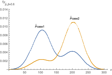
(a) for different values of $\widetilde{p}$

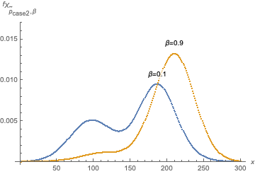
(b) for different values of $\beta$

Figure 4: Density function of the fuzzy GMM newsvendor

It is worthwhile to notice that the higher the risk parameter $\beta$ is, the more important the second demand mode is when compared to the first mode. As a consequence, the value $\beta$ chosen by the decision maker impacts the order quantity and the associated profit expectation as well as the profit variance. Indeed the choice made by the decision maker of the parameter $\beta$ drives the importance s/he gives to the right or the left side legs of the fuzzy number $\widetilde{p}$. Indeed, the average $\mathbb{E}[X_{\widetilde{p},\beta}]=\int_{-\infty}^{+\infty}xf_{X_{\widetilde{p},\beta}}(x)\,dx$ as well as the variance $\mathrm{Var}[X_{\widetilde{p},\beta}]=\int_{-\infty}^{+\infty}(x-\mathbb{E}[X_{\widetilde{p},\beta}])^{2}f_{X_{\widetilde{p},\beta}}(x)\,dx$ of the demand distribution $X_{\widetilde{p},\beta}$ are directly linked to $\beta$. As illustrated in Figure 5, as intuitively expected, the expected demand resulting from the fuzzy GMM is increasing with $\beta$ since for higher $\beta$, the decision maker tends to give more importance to the right side leg of the distribution of $\widetilde{p}$. Less intuitively, the variance of the fuzzy GMM demand is not necessarily in its lowest value for the risk neutral case (i.e. for $\beta=0.5$) and might be lower in the extreme situations with risk-averse and risk-seeking choices of $\beta$. Obviously, the standard deviations of the probability distributions $\sigma_{1}$ and $\sigma_{2}$ impact directly the variance of the fuzzy GMM as illustrated in Figure 5(b), but they have a low impact on the expected values as depicted in Figure 5(a).

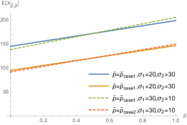
(a) Expected Demand

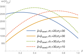
(b) Demand Variance

Figure 5: Expectation and Variance of the fuzzy GMM demand

In order to highlight the added value of the fuzzy GMM modelling, one can assume that the decision maker might adopt three ways to handle the mixture of the two probabilistic demands weighted by the fuzzy number $\widetilde{p}$:

• Ignoring one of the probability distributions by setting $p=0$ or $p=1$: these two cases model for instance a decision maker fully trusting or not the impact of past customer reviews on sales. Classical newsvendor solutions are then used here by considering as a demand density function either $f_{1}$ for $p=1$ or $f_{2}$ for $p=0$.

• Averaging the fuzzy number $\widetilde{p}$ and then considering a GMM with a non fuzzy weight $p=E[\widetilde{p}]$ (as detailed in Section 4.1). This case corresponds to the framework developed by Rekik et al. (2017) by setting the Bernoulli parameter of their model equal to $E[\widetilde{p}]$.

• Considering a fuzzy GMM with $\widetilde{p}=(p_{1},p_{2},p_{3},p_{4})$, then choosing a risk factor $\beta$ and deriving the associated order quantity as developed in the present paper.

For each case, the order quantity is calculated: $Q^{*}_{p=0}$ if $p=0$, $Q^{*}_{p=1}$ if $p=1$, $Q^{*}_{p=E[\widetilde{p}]}$ if $p=E[\widetilde{p}]$ and $Q^{*}_{\widetilde{p},\beta}$ if $\widetilde{p}=(p_{1},p_{2},p_{3},p_{4})$ for a given risk factor $\beta$. Then, the profit performance pertaining to each order quantity are derived by using the excepted profit and the profit variance of the fuzzy GMM $\mathbb{E}[\pi(X_{\widetilde{p},\beta})](\cdot)$, $\mathrm{Var}[\pi(X_{\widetilde{p},\beta})](\cdot)$, applied to each order quantity.

Since $\mathbb{E}[\pi(X_{\widetilde{p},\beta})](\cdot)$ is optimized if the order quantity is set equal to $Q^{*}_{\widetilde{p},\beta}$, the three other cases, i.e. when the order quantities are equal to $Q^{*}_{p=j}$ $(j=0,1,E[\widetilde{p}])$, which are then sub-optimal. We calculate their deviation from the optimal solution by using the following profit expectation ratios for $j=(0,1,E[\widetilde{p}])$:

$$\textrm{Benefit of the fuzzy GMM}=\frac{\mathbb{E}[\pi(X_{\widetilde{p},\beta})](Q^{*}_{\widetilde{p},\beta})-\mathbb{E}[\pi(X_{\widetilde{p},\beta})](Q^{*}_{p=j})}{\mathbb{E}[\pi(X_{\widetilde{p},\beta})](Q^{*}_{p=j})}.$$

Similarly, for each $j=(0,1,E[\widetilde{p}])$, we investigate the implication on the profit variance by using the following expression:

$$\textrm{Profit variance change}=\frac{\mathrm{Var}[\pi(X_{\widetilde{p},\beta})](Q^{*}_{\widetilde{p},\beta})-\mathrm{Var}[\pi(X_{\widetilde{p},\beta})](Q^{*}_{p=j})}{\mathrm{Var}[\pi(X_{\widetilde{p},\beta})](Q^{*}_{p=j})}.$$

Figures 6 and 7 compare the order quantities under the different values taken by $p$ for the high and low margin cost assumptions. Since $\mathbb{E}[X_{\widetilde{p},\beta}]$ is increasing with $\beta$ as illustrated in Figure 5(a), the optimal order quantity of the fuzzy GMM, $Q^{*}_{\widetilde{p},\beta}$, increases with $\beta$ consequently. The slope of such increase is directly linked to the impact of $\beta$ on the demand variance $\mathrm{Var}[X_{\widetilde{p},\beta}]$ showed in Figure 5(b), but also to the cost structure of the product. While it is straightforward to analytically and numerically observe that the order quantity $Q^{*}_{p=E[\widetilde{p}]}$ is ranging between $Q^{*}_{p=0}$ and $Q^{*}_{p=1}$, this is not the case for $Q^{*}_{p=E[\widetilde{p}]}$ which could fall outside this range for the extreme values of $\beta$. This is due to the fact that $Q^{*}_{p=\widetilde{p}}$ involves not only the expectation of the fuzzy number $\widetilde{p}$ but also its variability. It is known in the newsvendor literature that the order quantity increases (decreases) with the demand variance for high (low) margin cost structure. The graph pertaining to the case $p=E[\widetilde{p}]$ crosses the fuzzy GMM one for $\beta=0.5$: as discussed in Remark 4.2, averaging the fuzzy number $\widetilde{p}$ and using this average as a weight parameter is a particular case of our fuzzy GMM problem.

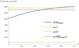
(a) $\widetilde{p}=\widetilde{p}_{case1}$

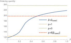
(b) $\widetilde{p}=\widetilde{p}_{case2}$

Figure 6: Order quantity - high margin cost structure

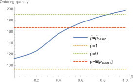
(a) $\widetilde{p}=\widetilde{p}_{case1}$

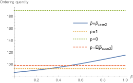
(b) $\widetilde{p}=\widetilde{p}_{case2}$

Figure 7: Order quantity - low margin cost structure

By applying the fuzzy GMM for values of $\beta$ ranging from 0 to 1, the decision maker expects increasing profit for increasing $\beta$ as depicted in Figures 8(a) and 9(a): moving the cursor onto the right side of the fuzzy number increases the demand expectation and hence the profit expectation. Surprisingly, the profit variance (depicted in Figures 8(b) and 9(b)) is however not a monotonous function of $\beta$ nor a convex function with a higher profit variance at the extreme values of $\beta$. In the contrast, it is worthwhile to notice that setting the $\beta$ around $0.5$, i.e. by giving similar importance to the left and right legs of the fuzzy number $\widetilde{p}$, does not lead to a lower profit variance. For $\widetilde{p}_{case1}=(0.1,0.2,0.4,0.4)$, the profit variance is in its lowest value for $\beta=1$ under the high margin assumption and for $\beta=0$ under the low margin case and the result is reversed for $\widetilde{p}_{case2}=(0.6,0.7,0.9,0.95)$. By combining the outcome illustrated in the (a) and (b) sides of Figures 8 and 9, the decision maker is able to choose the appropriate value of $\beta$ trading off its impact on the expectation and variance of the profit. Depending on the problem parameters, there are cases, such as $\widetilde{p}_{case1}$ and high margin cost structure, where a choice of $\beta=1$ is beneficial for both the profit expectation and variance. There are also cases where a $\beta$ not in the extreme values is to be chosen depending on the risk sensitivity of the decision maker.

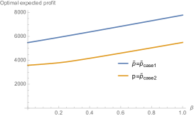
(a) Profit expectation

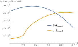
(b) Profit variance

Figure 8: Optimal Profit - high margin cost structure

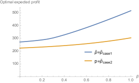
(a) Profit expectation

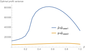
(b) Profit variance

Figure 9: Optimal Profit - low margin cost structure

As intuitively expected, Figure 10 shows that totally ignoring one of the probabilistic demand distributions leads to significant loss (up to $80\%$ for $\widetilde{p}_{case1}$, low margin) compared to the case where the two distributions are mixed with a fuzzy number. This is a key message to practitioners who are facing increasing impact of social media, expert evaluation, and customer feedback on their statistical demand forecasts.

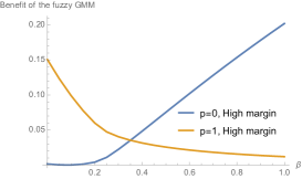
(a) Under case 2 $\widetilde{p}_{case2}=(0.6,0.7,0.9,0.9)$

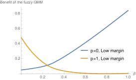
(b) Under case 1 $\widetilde{p}_{case2}=(0.1,0.2,0.4,0.4)$

Figure 10: Benefit of the fuzzy GMM if $p$ is set equal to 0 and 1

As mentioned above, the case where the fuzzy number $\widetilde{p}$ is averaged and the average $E[\widetilde{p}]$ is used as a weight of the GMM is a particular case of our fuzzy GMM problem. In order to measure the benefit related to the use of the fuzzy GMM instead of a GMM with a weight equal to the average of the fuzzy number, we compare the expected profit and profit variance in both cases. Since one is a particular case of the other, it is straightforward to observe a positive impact on the expected profit when using the fuzzy GMM (as illustrated in Figure 11). More importantly, the benefit is quite meaningful particularly for the low margin cost assumption. Since, low margin products are sensitive to overstock penalties, the fuzzy GMM permits to fine tune the demand estimation with the factor $\beta$ and consequently to limit the overstock risk.

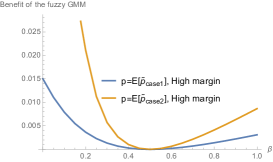
(a) Under the high margin cost

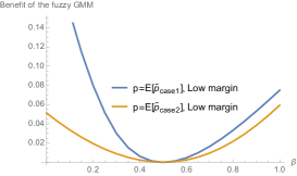
(b) Under the low margin cost

Figure 11: Benefit of the fuzzy GMM if $p$ is set equal $p=E[\widetilde{p}]$

Figure 12 shows that adopting the $\beta=0.5$ with an indifferent importance of the right and left legs of the fuzzy number $\widetilde{p}$ can lead to a significant decrease of the profit variance under the risk-seeking profile of the decision maker. It is also worthwhile to notice a non-monotonous behavior of the profit variance impact.

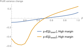
(a) Under case 2 $\widetilde{p}_{case2}=(0.6,0.7,0.9,0.9)$

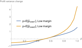
(b) Under case 1 $\widetilde{p}_{case1}=(0.1,0.2,0.4,0.4)$

Figure 12: Profit variance change of the fuzzy GMM if $p$ is set equal to $p=E[\widetilde{p}]$

6 Conclusion

Inspired by the increasing exposition of decision makers to both statistical and judgemental based sources of demand information, we developed in this paper a fuzzy GMM framework for the newsvendor permitting to mix probabilistic inputs with a subjective weight modelled as a fuzzy number. Thanks to a tractable mathematical application of the fuzzy machinery on the newsvendor problem, we derived the optimal ordering strategy taking into account both probabilistic and fuzzy components of the demand. We then reverse engineered the result to show that the fuzzy GMM problem could be interpreted as a classical newsvendor problem with a modified density function involving all the parameters of the probabilistic density functions and the legs of the fuzzy number. That is, mixing the different demand components could be interpreted as a requirement to revise the inventory policy by revisiting the ordering strategy of the newsvendor problem or a requirement to revise the forecasting exercise and then applying the classical newsvendor problem on the adjusted forecast outcome. The numerical study of the paper fitly provided the rationale of the use of fuzzy weight to the GMM. Customers sensitivity to review feedback or experts opinions is typically a perfect case study where customers demand is impacted by a fuzzy weighted GMM. The second part of the numerical study showed the applicability of the developed model and pointed out its added value compared to practices where the weights are either ignored or set equal to an average value avoiding then to integrate its variability in the inventory policy. The developed model permitted to show unusual multi-modal demand assumptions for the newsvendor problem and integrated the risk measure on the profit. As a future research agenda, one can target the extension of the model to a multi-period setting of the problem with a learning curve on the fuzzy number over periods. Indeed, the fuzzy weight was supposed to be known accurately in this paper which needs a learning exercise on the judgemental based component of the demand.

References

• Agrawal and Seshadri (2000) Agrawal, V., Seshadri, S., 2000. Impact of Uncertainty and Risk Aversion on Price and Order Quantity in the Newsvendor Problem. Manufacturing & Service Operations Management 2, 410–423. URL: http://pubsonline.informs.org/doi/abs/10.1287/msom.2.4.410.12339, doi:10.1287/msom.2.4.410.12339.
• Arrow et al. (1951) Arrow, K., Harris, T., Marshak, J., 1951. Optimal inventory policy. Econometrica 19, 250 – 272.
• Bertsimas and Thiele (2014) Bertsimas, D., Thiele, A., 2014. Robust and data-driven optimization: Modern decision making under uncertainty, in: Arrow, K., Karlin, S., Scarf, H. (Eds.), tutorials in Operations Research. INFORMS PubsOnline. chapter 5, pp. 95 – 122.
• Chen and Ho (2011) Chen, S.P., Ho, Y.H., 2011. Analysis of the newsboy problem with fuzzy demands and incremental discounts. International Journal of Production Economics 129, 169–177. URL: http://www.sciencedirect.com/science/article/pii/S092552731000352X, doi:10.1016/j.ijpe.2010.09.014.
• Choi et al. (2008) Choi, T., Li, D., Yan, H., 2008. Mean–variance analysis for the newsvendor problem. IEEE Transactions on Systems, Man, and Cybernetics - Part A: Systems and Humans 38, 1169 – 1180.
• Dutta and Chakraborty (2010) Dutta, P., Chakraborty, D., 2010. Incorporating one-way substitution policy into the newsboy problem with imprecise customer demand. European Journal of Operational Research 200, 99–110. URL: https://ideas.repec.org/a/eee/ejores/v200y2010i1p99-110.html.
• Gallego and Moon (1993) Gallego, G., Moon, I., 1993. The Distribution Free Newsboy Problem: Review and Extensions. The Journal of the Operational Research Society 44, 825–834. URL: https://www.jstor.org/stable/2583894, doi:10.2307/2583894.
• Guo and Ma (2014) Guo, P., Ma, X., 2014. Newsvendor models for innovative products with one-shot decision theory. European Journal of Operational Research 239, 523–536. URL: https://linkinghub.elsevier.com/retrieve/pii/S0377221714004512, doi:10.1016/j.ejor.2014.05.028.
• Hanasusanto et al. (2015) Hanasusanto, G.A., Kuhn, D., Wallace, S.W., Zymler, S., 2015. Distributionally robust multi-item newsvendor problems with multimodal demand distributions. Mathematical Programming 152, 1–32. URL: http://link.springer.com/10.1007/s10107-014-0776-y, doi:10.1007/s10107-014-0776-y.
• Kamburowski (2014) Kamburowski, J., 2014. The distribution-free newsboy problem under the worst-case and best-case scenarios. European Journal of Operational Research 237, 106–112. URL: https://linkinghub.elsevier.com/retrieve/pii/S0377221714001131, doi:10.1016/j.ejor.2014.01.066.
• Kholidasari and Ophiyandri (2018) Kholidasari, I., Ophiyandri, T., 2018. A Review of Human Judgment in Stock Control System for Disaster Logistics. Procedia Engineering 212, 1319–1325. URL: http://www.sciencedirect.com/science/article/pii/S187770581830198X, doi:10.1016/j.proeng.2018.01.170.
• Khouja (1999) Khouja, M., 1999. The single-period (news-vendor) problem: literature review and suggestions for future research. Omega 27, 537 – 553.
• Lee et al. (2015) Lee, C.Y., Li, X., Yu, M., 2015. The loss-averse newsvendor problem with supply options: The loss-averse newsvendor problem. Naval Research Logistics (NRL) 62, 46–59. URL: http://doi.wiley.com/10.1002/nav.21613, doi:10.1002/nav.21613.
• Lee and Nahmias (1993) Lee, H., Nahmias, S., 1993. Single-product, single-location models, in: Graves, SC, K., AHGR, Zipkin, P. (Eds.), Handbook in operations research and management science, volume on logistics of production and inventory. Elsevier, pp. 3 – 55.
• Li et al. (2002) Li, L., Kabadi, S.N., Nair, K.P.K., 2002. Fuzzy models for single-period inventory problem. Fuzzy Sets and Systems 132, 273–289. URL: http://www.sciencedirect.com/science/article/pii/S0165011402001045, doi:10.1016/S0165-0114(02)00104-5.
• Liu and Liu (2000) Liu, B., Liu, Y., 2000. Expected value of fuzzy variable and fuzzy expected value models. IEEE Transactions on Fuzzy Systems 10.
• Petrović et al. (1996) Petrović, D., Petrović, R., Vujošević, M., 1996. Fuzzy models for the newsboy problem. International Journal of Production Economics 45, 435–441. URL: http://www.sciencedirect.com/science/article/pii/092552739600014X, doi:10.1016/0925-5273(96)00014-X.
• Porteus (1990) Porteus, E., 1990. Stochastic inventory model, in: Graves, SC, K., AHGR, Zipkin, P. (Eds.), Handbook in operations research and management science, volume on stochastic models. Elsevier, pp. 605 – 652.
• Qin et al. (2011) Qin, Y., Wang, R., Vakharia, A.J., Chen, Y., Seref, M.M., 2011. The newsvendor problem: review and directions for future research. European Journal of Operational Research 213, 361 – 374.
• Rekik et al. (2017) Rekik, Y., Glock, C.H., Syntetos, A.A., 2017. Enriching demand forecasts with managerial information to improve inventory replenishment decisions: Exploiting judgment and fostering learning. European Journal of Operational Research 261, 182–194. URL: http://www.sciencedirect.com/science/article/pii/S0377221717301066, doi:10.1016/j.ejor.2017.02.001.
• Ryu and Yücesan (2010) Ryu, K., Yücesan, E., 2010. A fuzzy newsvendor approach to supply chain coordination. European Journal of Operational Research 200, 421–438. URL: http://www.sciencedirect.com/science/article/pii/S037722170900023X, doi:10.1016/j.ejor.2009.01.011.
• Salganik et al. (2006) Salganik, M.J., Dodds, P.S., Watts, D.J., 2006. Experimental Study of Inequality and Unpredictability in an Artificial Cultural Market. Science 311, 854–856. URL: https://science.sciencemag.org/content/311/5762/854, doi:10.1126/science.1121066.
• Scarf (1958) Scarf, H., 1958. A min-max solution of an inventory problem, in: Arrow, K., Karlin, S., Scarf, H. (Eds.), Studies in the Mathematical Theory of Inventory and Production. Stanford University Press. chapter 12, pp. 201 – 209.
• Syntetos et al. (2016) Syntetos, A.A., Kholidasari, I., Naim, M.M., 2016. The effects of integrating management judgement into OUT levels: In or out of context? European Journal of Operational Research 249, 853–863. URL: http://www.sciencedirect.com/science/article/pii/S0377221715006542, doi:10.1016/j.ejor.2015.07.021.
• Wang and Webster (2009) Wang, C., Webster, S., 2009. The loss-averse newsvendor problem. Omega 37, 93–105. URL: https://linkinghub.elsevier.com/retrieve/pii/S030504830600106X, doi:10.1016/j.omega.2006.08.003.
• Wang et al. (2012) Wang, C., Webster, S., Zhang, S., 2012. Newsvendor models with alternative risk preferences within expected utility theory and prospect theory frameworks, in: Choi, T. (Ed.), Handbook of newsvendor problems: models, extensions and applications. Springer. International Series in Operations Research and Management Science, pp. 177–196.
• Wang et al. (2009) Wang, C.X., Webster, S., Suresh, N.C., 2009. Would a risk-averse newsvendor order less at a higher selling price? European Journal of Operational Research 196, 544–553. URL: https://linkinghub.elsevier.com/retrieve/pii/S0377221708003500, doi:10.1016/j.ejor.2008.04.002.
• Wu et al. (2009) Wu, J., Wang, S., Cheng, T., 2009. Mean–variance analysis of the newsvendor model with stockout cost. Omega 37, 724 – 730.
• Wu et al. (2013) Wu, M., Zhu, S.X., Teunter, R.H., 2013. The risk-averse newsvendor problem with random capacity. European Journal of Operational Research 231, 328–336. URL: https://linkinghub.elsevier.com/retrieve/pii/S037722171300461X, doi:10.1016/j.ejor.2013.05.044.
• Xu and Zhai (2008) Xu, R., Zhai, X., 2008. Optimal models for single-period supply chain problems with fuzzy demand. Information Sciences 178, 3374–3381. URL: http://www.sciencedirect.com/science/article/pii/S0020025508001588, doi:10.1016/j.ins.2008.05.012.
• Yue et al. (2006) Yue, J., Chen, B., Wang, M.C., 2006. Expected Value of Distribution Information for the Newsvendor Problem. Operations Research 54, 1128–1136. URL: https://www.jstor.org/stable/25147042.