Gradient Flow Formulation of Diffusion equations in the Wasserstein Space over a Metric Graph

Abstract.

This paper contains two contributions in the study of optimal transport on metric graphs. Firstly, we prove a Benamou–Brenier formula for the Wasserstein distance, which establishes the equivalence of static and dynamical optimal transport. Secondly, in the spirit of Jordan–Kinderlehrer–Otto, we show that McKean–Vlasov equations can be formulated as gradient flow of the free energy in the Wasserstein space of probability measures. The proofs of these results are based on careful regularisation arguments to circumvent some of the difficulties arising in metric graphs, namely, branching of geodesics and the failure of semi-convexity of entropy functionals in the Wasserstein space.

1. Introduction

This article deals with the equivalence of static and dynamical optimal transport on metric graphs, and with a gradient flow formulation of McKean–Vlasov equations in the Wasserstein space of probability measures.

Let $(\mathsf{V},\mathsf{E})$ be a finite (undirected) connected graph and let $\ell:\mathsf{E}\to(0,\infty)$ be a given weight function. Loosely speaking, the associated metric graph is the geodesic metric space $({\mathfrak{G}},\mathsf{d})$ obtained by identifying the edges $e\in\mathsf{E}$ with intervals of length $\ell_{e}$, and gluing the intervals together at the nodes. In other words, a metric graph describes a continuous “cable system”, rather than a discrete set of nodes; see Section 2.2 for a more formal definition. Metric graphs arise in many applications in chemistry, physics, or engineering, describing quasi-one-dimensional systems such as carbon nano-structures, quantum wires, transport networks, or thin waveguides. They are also widely studied in mathematics; see [6, 23] for an overview.

For $1\leq p<\infty$, the $L^{p}$-Wasserstein distance $W_{p}$ between Borel probability measures $\mu$ and $\nu$ on ${\mathfrak{G}}$ is defined by the Monge–Kantorovich transport problem

$$W_{p}(\mu,\nu):=\min_{\sigma\in\Pi(\mu,\nu)}\bigg{\{}\int_{{\mathfrak{G}}\times{\mathfrak{G}}}\mathsf{d}^{p}(x,y)\,\mathrm{d}\sigma(x,y)\bigg{\}}^{1/p},$$

where $\Pi(\mu,\nu)$ denotes the set of transport plans; i.e., all Borel probability measures $\sigma$ on ${\mathfrak{G}}\times{\mathfrak{G}}$ with respective marginals $\mu$ and $\nu$. Since ${\mathfrak{G}}$ is compact, the Wasserstein distance $W_{p}$ metrises the topology of weak convergence of Borel probability measures on ${\mathfrak{G}}$, for any $p\geq 1$. The resulting metric space of probability measures is the $L^{p}$-Wasserstein space over ${\mathfrak{G}}$.

Metric graphs $({\mathfrak{G}},\mathsf{d})$ are prototypical examples of metric spaces that exhibit branching of geodesics: it is (typically) possible to find two distinct constant speed geodesics $(\gamma_{t})_{t\in[0,1]}$ and $(\tilde{\gamma}_{t})_{t\in[0,1]}$, taking the same values for all times $t\in[0,t_{0}]$ up to some $t_{0}\in(0,1)$. For this reason, several key results from optimal transport are not directly applicable to metric graphs. This paper contains two of these results.

The Benamou–Brenier formula

On Euclidean space $\mathbb{R}^{d}$, a dynamical characterisation of the Wasserstein distance has been obtained in celebrated works of Benamou and Brenier [4, 5]. The Benamou–Brenier formula asserts that

$$W_{2}^{2}(\mu,\nu)=\inf_{(\mu_{t},v_{t})}\Bigl{\{}\int_{0}^{1}{\left\|v_{t}\right\|}_{L^{2}(\mu_{t})}^{2}\,\mathrm{d}t\Bigr{\}}$$ (1.1)

where the infimum runs over all 2-absolutely continuous curves $(\mu_{t})_{t\in[0,1]}$ in the $L^{2}$-Wasserstein space over $\mathbb{R}^{d}$, satisfying the continuity equation

$$\frac{\,\mathrm{d}}{\,\mathrm{d}t}\mu_{t}+\nabla\cdot(v_{t}\mu_{t})=0$$ (1.2)

with boundary conditions $\mu_{0}=\mu$ and $\mu_{1}=\nu$.

Here we are interested in obtaining an analogous result in the setting of metric graphs. However, such an extension is not straightforward, since standard proofs in the Euclidean setting (see [2, 26]) make use of the flow map $T:[0,1]\times\mathbb{R}^{d}\to\mathbb{R}^{d}$ associated to a (sufficiently regular) vector field $(v_{t})_{t\in[0,1]}$, which satisfies

$$\frac{\,\mathrm{d}}{\,\mathrm{d}t}T(t,x)=v_{t}\big{(}T(t,x)\big{)},\qquad T(0,x)=x,\qquad T(t,\cdot)_{\#}\mu_{0}=\mu_{t},$$

see, e.g., [2, Proposition 8.1.8]. On a metric graph such a flow map $T$ typically fails to exist, since solutions $(\mu_{t})_{t\in[0,1]}$ to the continuity equation (1.2) are usually not uniquely determined by an initial condition $\mu_{0}$ and a given vector field $(v_{t})_{t\in[0,1]}$.

Circumventing this difficulty, Gigli and Han obtained a version of the Benamou–Brenier formula in very general metric measure spaces [13]. However, this paper requires a strong assumption on the measures (namely, a uniform bound on the density with respect to the reference measure). While this assumption is natural in the general setting of [13], it is unnecessarily restrictive in the particular setting of metric graphs.

In this paper, we prove a Benamou–Brenier formula that applies to arbitrary Borel probability measures on metric graphs. The key ingredient in the proof is a careful regularisation step for solutions to the continuity equation.

Gradient flow structure of diffusion equations

As an application of the Benamou–Brenier formula, we prove another central result from optimal transport: the identification of diffusion equations as gradient flow of the free energy in the Wasserstein space $({\mathcal{P}}({\mathfrak{G}}),W_{2})$. In the Euclidean setting, results of this type go back to the seminal work of Jordan, Kinderlehrer, and Otto [14].

Here we consider diffusion equations of the form

$$\partial_{t}\eta=\Delta\eta+\nabla\cdot\big{(}\eta\big{(}\nabla V+\nabla W[\mu]\big{)}\big{)},$$ (1.3)

for suitable potentials $V:{\mathfrak{G}}\to\mathbb{R}$ and $W:{\mathfrak{G}}\times{\mathfrak{G}}\to\mathbb{R}$. In analogy with the Euclidean setting, we show that this equation arises as the gradient flow equation for a free energy ${\mathcal{F}}:{\mathcal{P}}({\mathfrak{G}})\to(-\infty,+\infty]$ composed as the sum of entropy, potential, and interaction energies:

$${\mathcal{F}}(\mu) :=\int_{{\mathfrak{G}}}\eta(x)\log\eta(x)\,\mathrm{d}\lambda(x)+\int_{{\mathfrak{G}}}V(x)\eta(x)\,\mathrm{d}\lambda(x)$$

$$\qquad+\frac{1}{2}\int_{{\mathfrak{G}}\times{\mathfrak{G}}}W(x,y)\eta(x)\eta(y)\,\mathrm{d}\lambda(x)\,\mathrm{d}\lambda(y),$$

if $\mu=\eta\lambda$, where $\lambda$ denotes the Lebesgue measure on ${\mathfrak{G}}$.

A key difference compared to the Euclidean setting is that the entropy is not semi-convex along $W_{2}$-geodesics; see Section 4. This prevents us from applying “off-the-shelf” results from the theory of metric measure spaces. Instead, we present a self-contained proof of the gradient flow result. Its main ingredient is a chain rule for the entropy along absolutely continuous curves, which we prove using a regularisation argument.

Interestingly, we do not need to assume continuity of the potential $V$ at the vertices. Therefore our setting includes diffusion with possibly singular drift at the vertices.

The Wasserstein distance over metric graphs for $p=1$ has been studied in [20]. The focus is on the approximation of Kantorovich potentials using $p$-Laplacian type problems.

The recent paper [10] deals with dynamical optimal transport metrics on metric graphs. The authors start with the dynamical definition à la Benamou–Brenier and consider links to several other interesting dynamical transport distances. The current paper is complementary, as it shows the equivalence of static and dynamical optimal transport, and a gradient flow formulation for diffusion equations.

Various different research directions involving optimal transport and graphs exist. In particular, dynamical optimal transport on discrete graphs have been intensively studied in recent years following the papers [11, 19, 21]. The underlying state space in these papers is a discrete set of nodes rather than a gluing of one-dimensional intervals.

Another line of research deals with branched optimal transport, which is used to model phenomena such as road systems, communication networks, river basins, and blood flow. Here one starts with atomic measures in the continuum, and graphs emerge to describe paths of optimal transport [28, 7].

Organisation of the paper

In Section 2 we collect preliminaries on optimal transport and metric graphs. Section 3 is devoted to the continuity equation and the Benamou–Brenier formula on metric graphs. In particular, we present a careful regularisation procedure for solutions to the continuity equation. Section 4 contains an example which demonstrates the lack convexity of the entropy along $W_{2}$-geodesics in the setting of metric graphs. Section 5 deals with the gradient flow formulation of diffusion equations.

2. Preliminaries

In this section we collect some basic definitions and results from optimal transport and metric graphs.

2.1. Optimal transport

In this section we collect some basic facts on the family of $L^{p}$-Wasserstein distances on spaces of probability measures. We refer to [26, Chapter 5], [1, Chapter 2] or [27, Chapter 6] for more details.

Let $(X,d)$ be a compact metric space. The space of Borel probability measures on $X$ is denoted by ${\mathcal{P}}(X)$. The pushforward measure $T_{\#}\mu$ induced by a Borel map $T:X\to Y$ between two Polish spaces is defined by $(T_{\#}\mu)(A):=\mu(T^{-1}(A))$ for all Borel sets $A\subseteq Y$.

Definition 2.1 (Transport plans and maps).

1. A (transport) plan between probability measures $\mu,\nu\in{\mathcal{P}}(X)$ is a probability measure $\sigma\in{\mathcal{P}}(X\times X)$ with respective marginals $\mu$ and $\nu$, i.e.,

   $$(\operatorname{proj}_{1})_{\#}\sigma=\mu\qquad\text{and}\qquad(\operatorname{proj}_{2})_{\#}\sigma=\nu,$$

   where $\operatorname{proj}_{i}(x_{1},x_{2}):=x_{i}$ for $i=1,2$. The set of all transport plans between $\mu$ and $\nu$ is denoted by $\Pi(\mu,\nu)$.

2. A transport plan $\sigma\in\Pi(\mu,\nu)$ is said to be induced by a Borel measurable transport map $T:X\to X$ if $\sigma=({\operatorname{Id}},T)_{\#}\mu$, where $({\operatorname{Id}},T):X\to X\times X$ denotes the mapping $x\mapsto(x,T(x))$.

Definition 2.2 (Kantorovich–Rubinstein–Wasserstein distance).

For $p\geq 1$, the $L^{p}$-Kantorovich–Rubinstein–Wasserstein distance between probability measures $\mu,\nu\in{\mathcal{P}}(X)$ is defined by

$$W_{p}(\mu,\nu):=\inf\biggl{\{}\biggr{(}\int_{X\times X}d^{p}(x,y)\,\mathrm{d}\sigma(x,y)\biggr{)}^{1/p}:\sigma\in\Pi(\mu,\nu)\biggr{\}}.$$ (2.1)

For any $\mu,\nu\in{\mathcal{P}}(X)$ the infimum above is attained by some $\sigma_{\min}\in\Pi(\mu,\nu)$; any such $\sigma_{\min}$ is called an optimal (transport) plan between $\mu$ and $\nu$. If a transport map $T$ induces an optimal transport plan, we call $T$ optimal as well.

By compactness of $(X,d)$, the $L^{p}$-Wasserstein distance metrises the weak convergence in ${\mathcal{P}}(X)$ for any $p\geq 1$; see, e.g., [27, Corollary 6.13]. Moreover, $({\mathcal{P}}(X),W_{p})$ is a compact metric space as well.

We conclude this section with a dual formula for the Wasserstein distance (see, e.g., [26, Section 1.6.2]). To this aim, we recall that for $c:X\times X\to\mathbb{R}$, the $c$-transform of a function $\varphi:X\to{\mathbb{R}}\cup\{+\infty\}$ is defined by $\varphi^{c}(y):=\inf_{x\in X}c(x,y)-\varphi(x)$. A function $\psi:X\to{\mathbb{R}}\cup\{+\infty\}$ is called $c$-concave if there exists a function $\varphi:X\to{\mathbb{R}}\cup\{+\infty\}$ such that $\psi=\varphi^{c}$.

Proposition 2.3 (Kantorovich duality).

For any $\mu,\nu\in{\mathcal{P}}(X)$ we have

$$W_{p}^{p}(\mu,\nu)=\sup_{\varphi,\psi\in C(X)}\biggl{\{}\int_{X}\varphi\,\mathrm{d}\mu+\int_{X}\psi\,\mathrm{d}\nu\ :\ \varphi(x)+\psi(y)\leq d^{p}(x,y)\quad\forall x,y\in X\biggr{\}}.$$

Moreover, the supremum is attained by a maximising pair of the form $(\varphi,\psi)=(\varphi,\varphi^{c})$, where $\varphi$ is a $c$-concave function, for $c(x,y):=d^{p}(x,y)$.

Any maximiser $\varphi$ is called a Kantorovich potential.

2.2. Metric graphs

In this subsection we state some basic facts on metric graphs; see e.g., [20], [6] or [16] for more details.

Definition 2.4 (Metric graph).

Let $\mathsf{G}=(\mathsf{V},\mathsf{E},\ell)$ be an oriented, weighted graph, which is finite and connected. We identify each edge $e=(e_{\operatorname{init}},e_{\operatorname{term}})\in\mathsf{E}$ with an interval $(0,\ell_{e})$ and the corresponding nodes $e_{\operatorname{init}},e_{\operatorname{term}}\in\mathsf{V}$ with the endpoints of the interval, ($0$ and $\ell_{e}$ respectively). The spaces of open and closed metric edges over $\mathsf{G}$ are defined as the respective topological disjoint unions

$${\mathfrak{E}}:=\coprod_{e\in\mathsf{E}}(0,\ell_{e})\qquad\text{and}\qquad\overline{{\mathfrak{E}}}:=\coprod_{e\in\mathsf{E}}[0,\ell_{e}].$$

The metric graph over $\mathsf{G}$ is the topological quotient space

$${\mathfrak{G}}:=\faktor{\overline{{\mathfrak{E}}}}{\sim},$$

where points in $\overline{{\mathfrak{E}}}$ corresponding to the same vertex are identified.

Note that the orientation of $e$ determines the parametrisation of the edges, but does not otherwise play a role. To distinguish ingoing and outgoing edges at a given node, we introduce the signed incidence matrix $\mathcal{I}=(\iota_{ev})$ whose entries are given by

$$\iota_{ev}:=\begin{cases}+1\quad&\hbox{if }v=e_{\operatorname{init}},\\ -1&\hbox{if }v=e_{\operatorname{term}},\\ 0&\hbox{otherwise}.\end{cases}$$

As a quotient space, any metric graph naturally inherits the structure of a metric space from the Euclidean distance on its metric edges [9, Chapter 3]: indeed, under our standing assumption that ${\mathfrak{G}}$ is connected the quotient semi-metric $\mathsf{d}$ becomes a metric.

The distance $\mathsf{d}:{\mathfrak{G}}\times{\mathfrak{G}}\to[0,\infty)$ on ${\mathfrak{G}}$ can be more explicitly described as follows: For $x,y\in{\mathfrak{G}}$, let $\tilde{\mathsf{G}}=(\tilde{\mathsf{V}},\tilde{\mathsf{E}})$ be the underlying discrete graph obtained by adding new vertices at $x$ and $y$, and let $\mathsf{d}(x,y)$ be the weighted graph distance between $x$ and $y$ in $\tilde{\mathsf{G}}$, i.e.,

$$\mathsf{d}(x,y):=\min\sum_{i=1}^{n}\ell_{e_{i}},$$

where the minimum is taken over all sequences of vertices $x=x_{0},\dots,x_{n}=y$ in the extended graph $\tilde{\mathsf{G}}$ such that $x_{i-1}$ and $x_{i}$ are vertices of an edge $e_{i}\in\tilde{\mathsf{E}}$ for all $i=1,\dots,n$. In particular, if $x$ and $y$ are vertices in $\mathsf{G}$, no new nodes are added, and we recover the graph distance in the original graph. We refer to [23, Chapter 3] for details.

By construction, the distance function $\mathsf{d}$ metrises the topology of ${\mathfrak{G}}$. It is readily checked that $\mathsf{d}$ is a geodesic distance, i.e., each pair of points $x,y\in{\mathfrak{G}}$ can be joined by a curve of minimal length $\mathsf{d}(x,y)$. Consequently, also the Wasserstein space $({\mathcal{P}}({\mathfrak{G}}),W_{2})$ is a geodesic space.

In a metric space $(X,d)$, recall that the local Lipschitz constant of a function $f:X\to{\mathbb{R}}$ is defined by

$${\operatorname{lip}}(f)(x):=\limsup_{y\to x}\frac{{\left|f(y)-f(x)\right|}}{d(x,y)},$$

whenever $x\in X$ is not isolated, and $0$ otherwise. The (global) Lipschitz constant is defined by

$${\operatorname{Lip}}(f):=\sup_{y\neq x}\frac{{\left|f(y)-f(x)\right|}}{d(x,y)}.$$

If the underlying space $X$ is a geodesic space, we have ${\operatorname{Lip}}(f)=\sup_{x}{\operatorname{lip}}(f)(x)$.

At the risk of being redundant, we explicitly introduce a few relevant function spaces, although they are actually already fully determined by the metric measure structure of the metric graph ${\mathfrak{G}}$.

1. $C({\mathfrak{G}})$ denotes the space of continuous real-valued functions on ${\mathfrak{G}}$, endowed with the uniform norm ${\left\|\cdot\right\|}_{\infty}$.

2. $C^{k}(\overline{\mathfrak{E}})$ is the space of all functions $\varphi$ on $\overline{\mathfrak{E}}$ such that the restriction to each closed edge has continuous derivatives up to order $k\in{\mathbb{N}}$.

3. $L^{p}({\mathfrak{G}})$, for $p\in[1,\infty]$, is the $p$-Lebesgue space over the measure space $({\mathfrak{G}},\lambda)$, where $\lambda$ denotes the image of the 1-dimensional Lebesgue measure on $\overline{\mathfrak{E}}$ under the quotient map.

4. Likewise, we consider the Sobolev spaces $W^{1,p}(\overline{\mathfrak{E}})$ of $L^{p}({\mathfrak{G}})$-functions whose restriction on each edge is weakly differentiable with weak derivatives in $L^{p}({\mathfrak{G}})$.

3. The continuity equation on a metric graph

In this section we fix a metric graph ${\mathfrak{G}}$ and perform a study of the continuity equation

$$\partial_{t}\mu_{t}+\nabla\cdot J_{t}=0$$ (3.1)

in this context.

3.1. The continuity equation

In this work we mainly deal with weak solutions to the continuity equation, which will be introduced in Definition 3.2. To motivate this definition, we first introduce the following notion of strong solution.

Definition 3.1 (Strong solutions to the continuity equation).

A pair of measurable functions $(\rho,U)$ with $\rho:(0,T)\times{\mathfrak{G}}\to\mathbb{R}_{+}$ and $U:(0,T)\times\overline{{\mathfrak{E}}}\to\mathbb{R}$ is said to be a strong solution to (3.1) if

1. $t\mapsto\rho(t,x)$ is continuously differentiable for every $x\in{\mathfrak{G}}$;

2. $x\mapsto U_{t}(x)$ belongs to $C^{1}(\overline{\mathfrak{E}})$ for every $t\in(0,T)$;

3. the continuity equation $\frac{\mathrm{d}}{\mathrm{d}t}\rho_{t}(x)+\nabla\cdot U_{t}(x)=0$ holds for every $t\in(0,T)$ and $x\in{\mathfrak{E}}$;

4. for every $t\in(0,T)$ and $w\in\mathsf{V}$ we have $\sum_{e\in\mathsf{E}_{w}}\iota_{ew}U_{t}(w_{e})=0$.

Here, we write $\rho_{t}:=\rho(t,\cdot)$ and $U_{t}:=U(t,\cdot)$ and denote by $\nabla$ the spatial derivative. Moreover, $\mathsf{E}_{w}$ denotes the set of all edges adjacent to the node $w\in\mathsf{V}$, and $w_{e}\in\overline{{\mathfrak{E}}}$ denotes the corresponding endpoint of the metric edge $e$ which corresponds to $w\in{\mathfrak{G}}$.

To motivate the definition of a weak solution, suppose that we have a strong solution $(\rho_{t},U_{t})_{t\in(0,T)}$ to the continuity equation (3.1). Let $\psi\in C^{1}(\overline{\mathfrak{E}})\cap C({{\mathfrak{G}}})$ be a test function. Integration by parts on every metric edge $e$ gives

$$\frac{\mathrm{d}}{\mathrm{d}t}\int_{0}^{\ell_{e}}\psi\rho_{t}\,\mathrm{d}x=\int_{0}^{\ell_{e}}\nabla\psi\cdot U_{t}\,\mathrm{d}x+\psi U_{t}\Big{|}_{0}^{\ell_{e}},$$

and summation over $e\in\mathsf{E}$ yields

$$\frac{\mathrm{d}}{\mathrm{d}t}\int_{{\mathfrak{G}}}\psi\rho_{t}\,\mathrm{d}x=\int_{\overline{\mathfrak{E}}}\nabla\psi\cdot U_{t}\,\mathrm{d}x+\sum_{w\in\mathsf{V}}\psi(w)\sum_{e\in\mathsf{E}_{w}}\iota_{ew}U_{t}(w_{e})=\int_{\overline{\mathfrak{E}}}\nabla\psi\cdot U_{t}\,\mathrm{d}x,$$

where we use the continuity of $\psi$ on ${\mathfrak{G}}$ as well as the node condition (iv) above in the last step. This ensures that the net ingoing momentum vanishes at every node in $\mathsf{V}$. In particular, choosing $\psi\equiv 1$ yields

$$\int_{\mathfrak{G}}\rho_{s}\,\mathrm{d}\lambda=\int_{\mathfrak{G}}\rho_{t}\,\mathrm{d}\lambda,$$

for all $s,t\in(0,T)$, i.e. solutions to the continuity equation are mass-preserving. Here condition (iv) is crucial to ensure that no creation or annihilation of mass occurs at the nodes.

Definition 3.2 (Weak solution).

A pair $(\mu_{t},J_{t})_{t\in(0,T)}$ consisting of probability measures $\mu_{t}$ on ${\mathfrak{G}}$ and signed measures $J_{t}$ on $\overline{\mathfrak{E}}$, such that $t\mapsto\big{(}\mu_{t}(A),J_{t}(A)\big{)}$ is measurable for all Borel sets $A$, is said to be a weak solution to (3.1) if

1. $t\mapsto\int_{{\mathfrak{G}}}\psi\,\mathrm{d}\mu_{t}$ is absolutely continuous for every $\psi\in C^{1}(\overline{\mathfrak{E}})\cap C({{\mathfrak{G}}})$;

2. $\int_{0}^{T}|J_{t}|(\overline{\mathfrak{E}})\,\mathrm{d}t<\infty$;

3. for every $\psi\in C^{1}(\overline{\mathfrak{E}})\cap C({{\mathfrak{G}}})$ and a.e. $t\in(0,T)$, we have

   $$\frac{\mathrm{d}}{\mathrm{d}t}\int_{{\mathfrak{G}}}\psi\,\mathrm{d}\mu_{t}=\int_{\overline{\mathfrak{E}}}\nabla\psi\cdot\mathrm{d}J_{t}.$$ (3.2)

Remark 3.3.

Proposition 3.10 below shows that continuous functions on ${\mathfrak{G}}$ can be uniformly approximated by $C^{1}$ functions. By standard arguments it then follows that $(\mu_{t},J_{t})_{t\in(0,T)}$ is a weak solution if and only if the following conditions hold: $(i^{\prime})$ $t\mapsto\mu_{t}$ is weakly continuous; $(ii)$ from Definition 3.2 holds; and

1. for every $\varphi\in C^{1}_{c}\big{(}(0,T)\times\overline{\mathfrak{E}}\big{)}$ such that $\varphi_{t},\partial_{t}\varphi_{t}\in C^{1}(\overline{\mathfrak{E}})\cap C({{\mathfrak{G}}})$ for all $t\in(0,T)$ we have

   $$\int_{0}^{T}\!\biggl{(}\int_{{\mathfrak{G}}}\partial_{t}\varphi\,\mathrm{d}\mu_{t}+\int_{\overline{\mathfrak{E}}}\nabla\varphi\cdot\mathrm{d}J_{t}\biggr{)}\mathrm{d}t=0.$$ (3.3)

See Lemma 3.11 below for the weak continuity in $(i^{\prime})$.

The next result asserts that the momentum field does not give mass to vertices for a.e. time point. Hence, we can equivalently restrict the integrals over $\overline{{\mathfrak{E}}}$ in (3.2) and (3.3) to the space of open edges ${\mathfrak{E}}$.

Lemma 3.4.

Let $B:=\overline{\mathfrak{E}}\setminus{\mathfrak{E}}$ denote the set of all boundary points of edges. For any weak solution to the continuity equation $(\mu_{t},J_{t})_{t\in(0,T)}$, we have

$$\int_{0}^{T}|J_{t}|(B)\,\mathrm{d}t=0.$$

Proof.

Fix a metric edge $e$ in $\overline{\mathfrak{E}}$ and take $w\in\{e_{\rm init},e_{\rm term}\}$. Without loss of generality we take $w=e_{\rm init}$. Then we can construct a family of functions $\varphi_{\varepsilon}$ for $\varepsilon\in(0,\ell_{e})$ with the following properties:

1. $\varphi_{\varepsilon}\in C^{1}(\overline{\mathfrak{E}})\cap C({\mathfrak{G}})$;

2. $\varphi_{\varepsilon}\equiv 0$ on $\overline{\mathfrak{E}}\setminus e$ and $\varphi_{\varepsilon}\to 0$ uniformly on ${\mathfrak{G}}$ as $\varepsilon\to 0$;

3. $|\nabla\varphi_{\varepsilon}|=1$ on $(0,\varepsilon)\subset e$ and $|\nabla\varphi_{\varepsilon}|\to 0$ uniformly on compact subsets of $\overline{\mathfrak{E}}\setminus\{w\}$.

For instance, we could set $\varphi^{\varepsilon}(x):={\mathbbm{1}}_{e}(x)\eta_{\varepsilon}(x)$, where $\eta_{\varepsilon}:\mathbb{R}\to\mathbb{R}$ is a $C^{1}$ approximation of the function $x\mapsto\big{(}x\wedge\frac{\varepsilon(\ell_{e}-x)}{\ell_{e}-\varepsilon}\big{)}\vee 0$. Choosing $\varphi(t,x)=\varphi^{\varepsilon}(x)$ in (3.3), we obtain by passing to the limit $\varepsilon\to 0$ that $\int_{0}^{T}|J_{t}|(\{w\})\mathrm{d}t=0$. ∎

Lemma 3.5 (Weak and strong solutions).

The following assertions hold:

1. If $(\rho_{t},U_{t})_{t\in(0,T)}$ is a strong solution to the continuity equation, then the pair $(\mu_{t},J_{t})_{t\in(0,T)}$ defined by $\mu_{t}=\rho_{t}\lambda$ and $J_{t}=U_{t}\lambda$ is a weak solution to the continuity equation.

2. If $(\mu_{t},J_{t})_{t\in(0,T)}$ is a weak solution to the continuity equation (3.2) such that the densities $\rho_{t}:=\frac{\mathrm{d}\mu_{t}}{\mathrm{d}\lambda}$ and $U_{t}:=\frac{\mathrm{d}J_{t}}{\mathrm{d}\lambda}$ exist for all times $t\in(0,T)$ and satisfy the regularity conditions (i) and (ii) of Definition 3.1, then $(\rho_{t},U_{t})_{t\in(0,T)}$ is a strong solution to the continuity equation.

Proof.

Both claims are straightforward consequences of integration by parts on each metric edge in ${\mathfrak{E}}$. ∎

3.2. Characterisation of absolutely continuous curves

Let $(X,d)$ be a metric space and let $T>0$.

Definition 3.6.

For $p\geq 1$, we say that a curve $\gamma:(0,T)\to X$ is $p$-absolutely continuous if there exists a function $g\in L^{p}(0,T)$ such that

$$d(\gamma_{s},\gamma_{t})\leq\int_{s}^{t}g_{r}\,\mathrm{d}r\qquad\forall s,t\in(0,T):s\leq t.$$ (3.4)

The class of $p$-absolutely continuous curves is denoted by $AC^{p}\big{(}(a,b);(X,d)\big{)}$. For $p=1$ we simply drop $p$ in the notation. The notion of locally $p$-absolutely continuous curve is defined analogously.

Proposition 3.7.

Let $p\geq 1$. For every $p$-absolutely continuous curve $\gamma:(0,T)\to X$, the metric derivative defined by

$${\left|\dot{\gamma}\right|}(t):=\lim_{s\to t}\frac{d(\gamma_{s},\gamma_{t})}{{\left|s-t\right|}}$$

exists for a.e. $t\in(0,T)$ and $t\mapsto{\left|\dot{\gamma}\right|}(t)$ belongs to $L^{p}(0,T)$. The metric derivative ${\left|\dot{\gamma}\right|}(t)$ is an admissible integrand in the right-hand side of (3.4). Moreover, any other admissible integrand $g\in L^{p}(0,T)$ satisfies ${\left|\dot{\gamma}\right|}(t)\leq g(t)$ for a.e. $t\in(0,T)$.

Proof.

See, e.g., [2, Theorem 1.1.2]. ∎

The next result relates the metric derivative of $t\mapsto\mu_{t}$ to the $L^{2}(\mu_{t})$-norm of the corresponding vector fields $v_{t}$.

Theorem 3.8 (Absolutely continuity curves).

The following statements hold:

1. If $(\mu_{t})_{t\in(0,T)}$ is absolutely continuous in $({\mathcal{P}}({\mathfrak{G}}),W_{2})$, then there exists, for a.e. $t\in(0,T)$, a vector field $v_{t}\in L^{2}(\mu_{t})$ such that $\|v_{t}\|_{L^{2}(\mu_{t})}\leq|\dot{\mu}|(t)$ and $(\mu_{t},v_{t}\mu_{t})_{t\in(0,T)}$ is a weak solution to the continuity equation (3.2).

2. Conversely, if $(\mu_{t},v_{t}\mu_{t})_{t\in(0,T)}$ is a weak solution to the continuity equation (3.2) satisfying $\int_{0}^{1}\|v_{t}\|_{L^{2}(\mu_{t})}\,\mathrm{d}t<+\infty$, then $(\mu_{t})_{t\in(0,T)}$ is an absolutely continuous curve in $({\mathcal{P}}({\mathfrak{G}}),W_{2})$ and $|\dot{\mu}|(t)\leq\|v_{t}\|_{L^{2}(\mu_{t})}$ for a.e. $t\in(0,T)$.

Proof of (i).

We adapt the proof of [2, Theorem 8.3.1] to the setting of metric graphs.

The idea of the proof is as follows: On the space-time domain $Q:=(0,T)\times{\mathfrak{G}}$ we consider the Borel measure ${\bm{\mu}}:=\int_{0}^{T}\delta_{t}\otimes\mu_{t}\,\mathrm{d}t$ whose disintegration with respect to the Lebesgue measure on $(0,T)$ is given by $(\mu_{t})_{t\in(0,T)}$. To deal with the fact that gradients of smooth functions are multi-valued at the nodes, we define $\overline{\mu}_{t}\in{\mathcal{M}}_{+}(\overline{\mathfrak{E}})$ by $\overline{\mu}_{t}(A):=\sum_{e\in\mathsf{E}}\mu_{t}(A\cap\overline{e})$ for every Borel set $A\subseteq\overline{\mathfrak{E}}$. We then set $\overline{Q}:=(0,T)\times\overline{\mathfrak{E}}$ and define $\overline{\bm{\mu}}\in{\mathcal{M}}_{+}(\overline{Q})$ by $\overline{\bm{\mu}}:=\int_{0}^{T}\delta_{t}\otimes\overline{\mu}_{t}\,\mathrm{d}t$. (Note that mass at the nodes is counted multiple times). Consider the linear spaces of functions ${\mathcal{T}}$ and ${\mathcal{V}}$ given by

$${\mathcal{T}} :={\operatorname{span}}\bigg{\{}(0,T)\times{\mathfrak{G}}\ni(t,x)\mapsto a(t)\varphi(x)\ :\ a\in C_{c}^{1}(0,T),\,\varphi\in C^{1}(\overline{\mathfrak{E}})\cap C({\mathfrak{G}})\bigg{\}},$$

$${\mathcal{V}} :=\bigg{\{}(0,T)\times\overline{\mathfrak{E}}\ni(t,x)\mapsto\nabla_{x}\Phi(t,x)\ :\ \Phi\in{\mathcal{T}}\bigg{\}}.$$

The strategy is to show that the linear functional $L:{\mathcal{V}}\to{\mathbb{R}}$ given by

$$L(a\otimes\nabla\varphi):=-\int_{Q}\dot{a}(t)\varphi(x)\,\mathrm{d}{\bm{\mu}}(x,t),$$

is well-defined and $L^{2}(\overline{Q},\overline{\bm{\mu}})$-bounded with ${\left\|L\right\|}^{2}\leq\int_{0}^{T}{\left|\dot{\mu}\right|}^{2}(t)\,\mathrm{d}t$. Once this is proved, the Riesz Representation Theorem yields the existence of a vector field $\boldsymbol{v}$ in $\overline{{\mathcal{V}}}\subseteq L^{2}(\overline{Q},\overline{\bm{\mu}})$ such that $\|\boldsymbol{v}\|^{2}_{L^{2}(\overline{\bm{\mu}})}\leq\int_{0}^{T}{\left|\dot{\mu}\right|}^{2}(t)\,\mathrm{d}t$ and

$$-\int_{0}^{T}\dot{a}(t)\int_{\mathfrak{G}}\varphi(x)\mathrm{d}\mu_{t}(x)\,\mathrm{d}t=L(a\otimes\nabla\varphi)=\int_{0}^{T}a(t)\int_{\overline{{\mathfrak{E}}}}\nabla\varphi(x)v_{t}(x)\,\mathrm{d}\overline{\mu}_{t}(x)\,\mathrm{d}t$$ (3.5)

for $v_{t}:=\boldsymbol{v}(t,\cdot)$ and all $a\in C_{c}^{1}(0,T)$ and $\varphi\in C^{1}(\overline{\mathfrak{E}})\cap C({\mathfrak{G}})$.

Once this is done, we show that the momentum vector field $\boldsymbol{J}:=\boldsymbol{v}\cdot{\bm{\mu}}$ does not assign mass to boundary points in $\overline{\mathfrak{E}}$, so that $\boldsymbol{v}$ can be interpreted as an element in $L^{2}(Q,{\bm{\mu}})$ and the integration over vector fields can be restricted to ${\mathfrak{E}}$.

Step 1.  Fix a test function $\varphi\in C^{1}(\overline{\mathfrak{E}})\cap C({\mathfrak{G}})$ and consider the bounded and upper semicontinuous function $H:{\mathfrak{G}}\times{\mathfrak{G}}\to\mathbb{R}$ given by

$$H(x,y):=\begin{cases}\displaystyle{\operatorname{lip}}(\varphi)(x)&\text{if }x=y,\\ \displaystyle\frac{{\left|\varphi(x)-\varphi(y)\right|}}{\mathsf{d}(x,y)}&\text{if }x\neq y,\end{cases}$$

for $x,y\in{\mathfrak{G}}$. For $s,t\in(0,T)$, let $\sigma^{s\to t}\in\Pi(\mu_{s},\mu_{t})$ be an optimal plan. The Cauchy–Schwarz inequality yields

$$\bigg{|}\int_{\mathfrak{G}}\varphi\,\mathrm{d}\mu_{s}-\int_{\mathfrak{G}}\varphi\,\mathrm{d}\mu_{t}\bigg{|} \leq\int_{{\mathfrak{G}}\times{\mathfrak{G}}}\mathsf{d}(x,y)H(x,y)\,\mathrm{d}\sigma^{s\to t}(x,y)$$ (3.6)

$$\leq W_{2}(\mu_{s},\mu_{t})\bigg{(}\int_{{\mathfrak{G}}\times{\mathfrak{G}}}H^{2}(x,y)\,\mathrm{d}\sigma^{s\to t}(x,y)\bigg{)}^{1/2}.$$

As $\varphi$ is globally Lipschitz on ${\mathfrak{G}}$, we obtain

$$\Bigl{|}\int_{\mathfrak{G}}\varphi\,\mathrm{d}\mu_{s}-\int_{\mathfrak{G}}\varphi\,\mathrm{d}\mu_{t}\Bigr{|}\leq{\operatorname{Lip}}(\varphi)W_{2}(\mu_{s},\mu_{t})$$

and infer that the mapping $t\mapsto\int_{\mathfrak{G}}\varphi\,\mathrm{d}\mu_{t}$ is absolutely continuous, hence, differentiable outside of a null set $N_{\varphi}\subseteq(0,T)$.

Fix $t\in(0,T)$ and take a sequence $\{s_{n}\}_{n\in{\mathbb{N}}}$ converging to $t$. Since $\{\mu_{s_{n}}\}$ is weakly convergent, this sequence is tight. Consequently, $\{\sigma^{s_{n}\to t}\}_{n\in{\mathbb{N}}}$ is tight as well, and we may extract a subsequence converging weakly to some $\hat{\sigma}\in{\mathcal{P}}({\mathfrak{G}}\times{\mathfrak{G}})$. It readily follows that $\hat{\sigma}\in\Pi(\mu_{t},\mu_{t})$. Moreover, along the convergent subsequence, we have

$$\int_{{\mathfrak{G}}\times{\mathfrak{G}}}\mathsf{d}^{2}(x,y)\,\mathrm{d}\hat{\sigma}(x,y)\leq\liminf_{n\to\infty}\int_{{\mathfrak{G}}\times{\mathfrak{G}}}\mathsf{d}^{2}(x,y)\,\mathrm{d}\sigma^{s_{n}\to t}(x,y)=\liminf_{n\to\infty}W_{2}^{2}(\mu_{s_{n}},\mu_{t})=0,$$

which implies that $\hat{\sigma}=({\operatorname{Id}},{\operatorname{Id}})_{\#}\mu_{t}$.

Using this result and the upper-semicontinuity of $H$, it follows from (3.6) that

$$\limsup_{s\to t}\bigg{|}\frac{\int_{\mathfrak{G}}\varphi\,\mathrm{d}\mu_{s}-\int_{\mathfrak{G}}\varphi\,\mathrm{d}\mu_{t}}{s-t}\bigg{|} \leq{\left|\dot{\mu}\right|}(t)\limsup_{s\to t}\bigg{(}\int_{{\mathfrak{G}}\times{\mathfrak{G}}}H^{2}(x,y)\,\mathrm{d}\sigma^{s\to t}(x,y)\bigg{)}^{1/2}$$ (3.7)

$$\leq{\left|\dot{\mu}\right|}(t)\cdot{\left\|{\operatorname{lip}}(\varphi)\right\|}_{L^{2}(\mu_{t})}.$$

Step 2.  Take $\Phi\in{\mathcal{T}}$. Using dominated convergence, Fatou’s Lemma, and (3.7), we obtain

$$\bigg{|}\int_{Q}\frac{\mathrm{d}}{\mathrm{d}t}\Phi(x,t)\,\mathrm{d}{\bm{\mu}}(x,t)\bigg{|} =\lim_{h\searrow 0}\bigg{|}\frac{1}{h}\int_{Q}\Phi(x,t-h)-\Phi(x,t)\,\mathrm{d}{\bm{\mu}}(x,t)\bigg{|}$$ (3.8)

$$=\lim_{h\searrow 0}\bigg{|}\frac{1}{h}\int_{0}^{T}\bigg{(}\int_{\mathfrak{G}}\Phi(x,t)\,\mathrm{d}\mu_{t+h}(x)-\int_{\mathfrak{G}}\Phi(x,t)\,\mathrm{d}\mu_{t}(x)\bigg{)}\,\mathrm{d}t\bigg{|}$$

$$\leq\int_{0}^{T}{\left|\dot{\mu}\right|}(t)\cdot{\left\|{\operatorname{lip}}_{x}(\Phi)(\cdot,t)\right\|}_{L^{2}(\mu_{t})}\,\mathrm{d}t$$

$$\leq\bigg{(}\int_{0}^{T}{\left|\dot{\mu}\right|}^{2}(t)\,\mathrm{d}t\bigg{)}^{1/2}\bigg{(}\int_{Q}{\left|{\operatorname{lip}}_{x}(\Phi)(x,t)\right|}^{2}\,\mathrm{d}{\bm{\mu}}(x,t)\Bigr{)}^{1/2}.$$

Since $\int_{Q}|{\operatorname{lip}}_{x}(\Phi)(x,t)|^{2}\,\mathrm{d}{\bm{\mu}}(x,t)\leq\int_{\overline{Q}}|\nabla\Phi(x,t)|^{2}\,\mathrm{d}\overline{\bm{\mu}}(x,t)$, we infer that $L$ is well-defined and extends to a bounded linear functional on the closure of ${\mathcal{V}}$ in $L^{2}(\overline{Q},\overline{\bm{\mu}})$ with ${\left\|L\right\|}^{2}\leq\int_{0}^{T}{\left|\dot{\mu}\right|}^{2}(t)\,\mathrm{d}t$, which allows us to apply the Riesz Representation Theorem, as announced above.

In particular, (3.5) implies that $t\mapsto\int_{{\mathfrak{E}}}\nabla\varphi\cdot v_{t}\,\mathrm{d}\mu_{t}$ is a distributional derivative for $t\mapsto\int_{\mathfrak{G}}\varphi\,\mathrm{d}\mu_{t}$. Since the latter function is absolutely continuous and, therefore, belongs to the Sobolev space $W^{1,1}(0,T)$, we obtain

$$\frac{\mathrm{d}}{\mathrm{d}t}\int_{\mathfrak{G}}\varphi\,\mathrm{d}\mu_{t}=\int_{\overline{\mathfrak{E}}}\nabla\varphi\cdot v_{t}\,\mathrm{d}\mu_{t}\qquad\text{for a.e.\ }t\in(0,T).$$ (3.9)

We conclude that $(\mu_{t},v_{t})_{t\in(0,T)}$ solves the continuity equation in the weak sense. Lemma 3.4 implies that for a.e. $t$ the momentum field $J_{t}:=v_{t}\cdot\overline{\mu}_{t}$ does not give mass to any boundary point in $\overline{{\mathfrak{E}}}$ . Consequently, the spatial domain of integration on the right-hand side of (3.5) may be restricted to ${\mathfrak{E}}$.

Step 4.  It remains to verify (by a standard argument) the inequality relating the $L^{2}(\mu_{t})$-norm of the vector field $v_{t}$ to the metric derivative of $\mu_{t}$.

For this purpose, fix a sequence $(\boldsymbol{\varpi}_{i})_{i\in{\mathbb{N}}}$ of functions $\boldsymbol{\varpi}_{i}\in{\mathcal{V}}$ converging to $\boldsymbol{v}$ in $L^{2}(\overline{{\bm{\mu}}})$ as $i\to\infty$. For every compact interval $I\subseteq(0,T)$ and $a\in C^{1}(0,T)$ satisfying $0\leq a\leq 1$ and $\operatorname{supp}a=I$, we then obtain

$$\int_{Q}a(t){\left|\boldsymbol{v}(x,t)\right|}^{2}\,\mathrm{d}{\bm{\mu}}(x,t) =\lim_{i\to\infty}\int_{Q}a(t)\boldsymbol{\varpi}_{i}(x,t)\boldsymbol{v}(x,t)\,\mathrm{d}{\bm{\mu}}(x,t)$$

$$=\lim_{i\to\infty}L(a\boldsymbol{\varpi}_{i})\leq\Bigl{(}\int_{0}^{T}{\mathbbm{1}}_{I}{\left|\dot{\mu}_{t}\right|}^{2}\,\mathrm{d}t\Bigr{)}^{1/2}\lim_{i\to\infty}\Bigl{(}\int_{Q}{\mathbbm{1}}_{I}|\boldsymbol{\varpi}_{i}|^{2}\,\mathrm{d}{\bm{\mu}}\Bigr{)}^{1/2}$$

$$=\Bigl{(}\int_{0}^{T}{\mathbbm{1}}_{I}{\left|\dot{\mu}\right|}^{2}(t)\,\mathrm{d}t\Bigr{)}^{1/2}\Bigl{(}\int_{Q}{\mathbbm{1}}_{I}{\left|v\right|}^{2}\,\mathrm{d}{\bm{\mu}}\Bigr{)}^{1/2}.$$

Letting ${\left\|a-{\mathbbm{1}}_{I}\right\|}_{\infty}\to 0$, this inequality implies

$$\int_{I}\int_{\mathfrak{E}}{\left|v_{t}\right|}^{2}\,\mathrm{d}\mu_{t}\,\mathrm{d}t\leq\int_{I}{\left|\dot{\mu}\right|}^{2}(t)\,\mathrm{d}t.$$

Since $I\subseteq(0,T)$ is arbitrary, this implies that ${\left\|v_{t}\right\|}_{L^{2}(\mu_{t})}\leq{\left|\dot{\mu}\right|}(t)$ for a.e. $t\in(0,T)$. ∎

3.3. Regularisation of solutions to the continuity equation

Next we introduce a suitable spatial regularisation procedure for solutions to the continuity equation. This will be crucial in the proof of the second part of Theorem 3.8.

Let $\varepsilon>0$ be sufficiently small, i.e., such that $2\varepsilon$ is strictly smaller than the length of every edge in $\mathsf{E}$. We then consider the supergraph ${\mathfrak{G}}_{\operatorname{ext}}\supseteq{\mathfrak{G}}$ defined by adjoining an auxiliary edge $e^{\operatorname{ext}}_{v}$ of length $2\varepsilon$ to each node $v\in\mathsf{V}$ (see Figure 1). The corresponding set of metric edges will be denoted by ${\mathfrak{E}}_{\operatorname{ext}}\supset{\mathfrak{E}}$.

We next define a regularisation procedure for functions based on averaging. The crucial feature here is that non-centred averages are used, to ensure that the regularised function is continuous.

In the definition below, we parametrise each edge $e=(e_{\operatorname{init}},e_{\operatorname{term}})\in\mathsf{E}$ using the interval $(-\frac{\ell_{e}}{2},\frac{\ell_{e}}{2})$ instead of $(0,\ell_{e})$. The auxiliary edges $e^{\operatorname{ext}}_{e_{\operatorname{init}}}$ and $e^{\operatorname{ext}}_{e_{\operatorname{term}}}$ will then be identified with the intervals $(-\frac{\ell_{e}}{2}-2\varepsilon,-\frac{\ell_{e}}{2})$ and $(\frac{\ell_{e}}{2},\frac{\ell_{e}}{2}+2\varepsilon)$, respectively. We stress that for each vertex $v$, there is only one additional edge, but we use several different parametrisations for it – one for each edge incident in $v$.

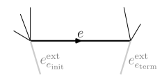
Figure 1. The supergraph ${\mathfrak{G}}_{\operatorname{ext}}$ is constructed by adjoining an additional leaf at every node in $V$.

Definition 3.9 (Regularisation of functions).

For $\varphi\in L^{1}({\mathfrak{G}}_{\operatorname{ext}})$, we define $\varphi^{\varepsilon}:{\mathfrak{G}}\to{\mathbb{R}}$ by

$$\varphi^{\varepsilon}(x):=\frac{1}{2\varepsilon}\int_{\alpha^{\varepsilon}_{e}x-\varepsilon}^{\alpha^{\varepsilon}_{e}x+\varepsilon}\varphi(y)\,\mathrm{d}y\qquad\text{for }x\in e=[-\tfrac{\ell_{e}}{2},\tfrac{\ell_{e}}{2}],$$ (3.10)

where $\alpha^{\varepsilon}_{e}:=(\ell_{e}+2\varepsilon)/\ell_{e}$. We write $\alpha^{\varepsilon}(x):=\alpha^{\varepsilon}_{e}$, whenever $x\in{\mathfrak{E}}$ is a point on the metric edge $e$.

Note that the value of $\varphi_{\varepsilon}$ in each of the nodes depends only on data on the corresponding auxiliary edge. In particular, the value at the nodes does not depend on the choice of the edge, so that $\varphi_{\varepsilon}$ indeed defines a function on ${\mathfrak{G}}$. We collect some basic properties of this regularisation in the following result.

Proposition 3.10.

The following properties hold for every $\varepsilon>0$ sufficiently small:

1. Regularising effect: For any $\varphi\in C({\mathfrak{G}}_{\operatorname{ext}})$ we have $\varphi^{\varepsilon}\in C^{1}(\overline{\mathfrak{E}})\cap C({{\mathfrak{G}}})$ and

   $$\nabla\varphi^{\varepsilon}(y)=\frac{\alpha^{\varepsilon}_{e}}{2\varepsilon}\bigl{(}\varphi(\alpha^{\varepsilon}_{e}y+\varepsilon)-\varphi(\alpha^{\varepsilon}_{e}y-\varepsilon)\bigr{)}$$ (3.11)

   for $y\in[-\ell_{e}/2,\ell_{e}/2]$.

2. If $\varphi$ belongs to $C({\mathfrak{G}}_{\operatorname{ext}})$, then $\varphi^{\varepsilon}$ converges uniformly to $\varphi|_{\mathfrak{G}}$ as $\varepsilon\searrow 0$.

Proof.

(i) follows by direct computation; (ii) follows using the uniform continuity of $\varphi$ on ${\mathfrak{G}}_{\operatorname{ext}}$. ∎

Lemma 3.11 (Weak continuity).

Let $(\rho_{t},J_{t})_{t\in(0,T)}$ be a weak solution to the continuity equation on ${\mathfrak{G}}$. Then $t\mapsto\int_{\mathfrak{G}}\varphi\,\mathrm{d}\mu_{t}$ is continuous for every $\varphi\in C({\mathfrak{G}})$.

Proof.

Fix $\varphi\in C({\mathfrak{G}})$, take a continuous extension to ${\mathfrak{G}}_{\operatorname{ext}}$, and define $\varphi^{\varepsilon}$ accordingly. Proposition 3.10.ii then implies that $\varphi^{\varepsilon}$ converges uniformly to $\varphi$ on ${\mathfrak{G}}$ as $\varepsilon\searrow 0$. As a result, the function $t\mapsto\int_{\mathfrak{G}}\varphi^{\varepsilon}\,\mathrm{d}\mu_{t}$ converges uniformly to $t\mapsto\int_{\mathfrak{G}}\varphi\,\mathrm{d}\mu_{t}$. Since $\varphi^{\varepsilon}$ belongs to $C({\mathfrak{G}})\cap C^{1}(\overline{\mathfrak{E}})$ by Proposition 3.10.i, we conclude that the mapping $t\mapsto\int_{\mathfrak{G}}\varphi\,\mathrm{d}\mu_{t}$ is continuous, being a uniform limit of continuous functions. ∎

By duality, we obtain a natural regularisation for measures.

Definition 3.12 (Regularisation of measures).

For $\mu\in{\mathcal{M}}({\mathfrak{G}})$ we define $\mu^{\varepsilon}\in{\mathcal{M}}({\mathfrak{G}}_{\operatorname{ext}})$ by

$$\int_{{\mathfrak{G}}_{\operatorname{ext}}}\varphi\,\mathrm{d}\mu^{\varepsilon}:=\int_{{\mathfrak{G}}}\varphi^{\varepsilon}\,\mathrm{d}\mu.$$ (3.12)

for all $\varphi\in C({\mathfrak{G}}_{\operatorname{ext}})$.

Analogously, for $J\in{\mathcal{M}}({\mathfrak{E}})$ we define $J^{\varepsilon}\in{\mathcal{M}}({\mathfrak{E}}_{\rm ext})$ as follows: first we extend $J$ to a measure on ${\mathfrak{G}}$ giving no mass to ${\mathfrak{G}}\setminus{\mathfrak{E}}$. Then we define $\tilde{J}_{\varepsilon}\in{\mathcal{M}}({\mathfrak{G}}_{\rm ext})$ by the formula above. Finally, we define $J_{\varepsilon}\in{\mathcal{M}}({\mathfrak{E}}_{\rm ext})$ by restriction of $\tilde{J}_{\varepsilon}$ to ${\mathfrak{E}}_{\rm ext}$.

It is readily checked that the right-hand side defines a positive linear functional on $C({\mathfrak{G}}_{\operatorname{ext}})$, so that $\mu^{\varepsilon}$ is indeed a well-defined measure.

Proposition 3.13.

The following properties hold for any $\varepsilon>0$:

1. Mass preservation: $\mu^{\varepsilon}({\mathfrak{G}}_{\operatorname{ext}})=\mu({\mathfrak{G}})$ for any $\mu\in{\mathcal{M}}({\mathfrak{G}})$.

2. Regularising effect: For any $\mu\in{\mathcal{P}}({\mathfrak{G}})$, the measure $\mu^{\varepsilon}$ is absolutely continuous with respect to $\lambda$ with density

   $$\rho^{\varepsilon}(x)=\left\{\begin{array}[]{ll}\displaystyle\frac{1}{2\varepsilon}\mu\big{(}e\cap I_{e}(x)\big{)},&\text{for $x$ on $e$ in ${\mathfrak{E}}$, }\\ \displaystyle\frac{1}{2\varepsilon}\bigg{(}{\mathbbm{1}}_{\{d(x,w)\leq 2\varepsilon\}}\mu(\{w\})+\sum_{e\in\mathsf{E}:w\in e}\mu\big{(}e\cap I_{e}(x)\big{)}\bigg{)},&\text{for $x$ on $e^{\operatorname{ext}}_{w}$, $w\in\mathsf{V},$}\end{array}\right.$$

   where

   $$I_{e}(x):=\left(\frac{x-\varepsilon}{a_{e}^{\varepsilon}}\vee\Big{(}-\frac{\ell_{e}}{2}\Big{)},\frac{x+\varepsilon}{a_{e}^{\varepsilon}}\wedge\frac{\ell_{e}}{2}\right).$$

   In particular, $\rho^{\varepsilon}(x)\leq\frac{1}{2\varepsilon}$ for all $x\in{\mathfrak{G}}_{\operatorname{ext}}$.

3. Kinetic energy bound: For $\mu\in{\mathcal{P}}({\mathfrak{G}})$ and $v\in L^{2}(\mu)$, define $J=v\mu|_{\mathfrak{E}}\in{\mathcal{M}}({\mathfrak{E}})$. Consider the regularised measures $\mu^{\varepsilon}\in{\mathcal{P}}({\mathfrak{G}}_{\operatorname{ext}})$ and $J^{\varepsilon}\in{\mathcal{M}}({\mathfrak{E}}_{\operatorname{ext}})$. Then we have $J^{\varepsilon}=v^{\varepsilon}\mu^{\varepsilon}$ for some $v^{\varepsilon}\in L^{2}(\mu^{\varepsilon})$ and

   $$\int_{{\mathfrak{E}}_{\operatorname{ext}}}{\left|v^{\varepsilon}\right|}^{2}\,\mathrm{d}\mu^{\varepsilon}\leq\int_{\mathfrak{E}}{\left|v\right|}^{2}\,\mathrm{d}\mu.$$ (3.13)

4. For any $\mu\in{\mathcal{P}}({\mathfrak{G}})$ we have weak convergence $\mu^{\varepsilon}\rightharpoonup\mu$ in ${\mathcal{P}}({\mathfrak{G}}_{\operatorname{ext}})$ as $\varepsilon\to 0$.

5. Let $(\mu_{t},J_{t})_{t\in(0,T)}$ be a weak solution to the to the continuity equation (3.2). Then the regularised pair $(\mu_{t}^{\varepsilon},J^{\varepsilon}_{t})_{t\in(0,T)}$ is a weak solution to a modified continuity equation on ${\mathfrak{G}}_{\operatorname{ext}}$ in the following sense:

   For every absolutely continuous function $\varphi$ on ${\mathfrak{G}}_{\operatorname{ext}}$, the function $t\mapsto\int_{{\mathfrak{G}}_{\operatorname{ext}}}\varphi\,\mathrm{d}\mu_{t}^{\varepsilon}$ is absolutely continuous and for a.e. $t\in(0,T)$ we have

   $$\frac{\mathrm{d}}{\mathrm{d}t}\int_{{\mathfrak{G}}_{\operatorname{ext}}}\varphi\,\mathrm{d}\mu_{t}^{\varepsilon}=\int_{{\mathfrak{E}}_{\operatorname{ext}}}\alpha^{\varepsilon}\nabla\varphi\cdot\,\mathrm{d}J_{t}^{\varepsilon},$$ (3.14)

   with $\alpha^{\varepsilon}$ as in Definition 3.9.

In order to prove (iii), we will make use of the so-called Benamou–Brenier functional (see, e.g., [26, Section 5.3.1] for corresponding results in the Euclidean setting).

Define $K_{2}:=\{(a,b)\in{\mathbb{R}}\times{\mathbb{R}}:a+b^{2}/2\leq 0\}$. By a slight abuse of notation, $C({\mathfrak{G}},K_{2})$ (resp. $L^{\infty}({\mathfrak{G}},K_{2})$) denotes the set of all continuous (resp. bounded and measurable) functions $a,b:{\mathfrak{G}}\to{\mathbb{R}}$ such that $a+b^{2}/2\leq 0$.

Definition 3.14.

The Benamou–Brenier functional ${\mathcal{B}}_{2}:{\mathcal{M}}({\mathfrak{G}})\times{\mathcal{M}}({\mathfrak{E}})\to{\mathbb{R}}\cup\{+\infty\}$ is defined by

$${\mathcal{B}}_{2}(\mu,J):=\sup_{(a,b)\in C({\mathfrak{G}},K_{2})}\bigg{\{}\int_{\mathfrak{G}}a\,\mathrm{d}\mu+\int_{\mathfrak{E}}b\,\mathrm{d}J\bigg{\}}.$$

Some basic properties of this functional are collected in the following lemma.

Lemma 3.15.

The following statements hold:

1. For $y,z\in\mathbb{R}$ we have

   $$\alpha(z,y):=\sup_{(a,b)\in K_{2}}\{az+by\}=\begin{cases}\displaystyle\frac{{\left|y\right|}^{2}}{2z}&\text{if }z>0,\\ 0&\text{if }z=0\text{ and }y=0,\\ +\infty&\text{otherwise.}\end{cases}$$ (3.15)

2. For $\mu\in{\mathcal{M}}({\mathfrak{G}})$ and $J\in{\mathcal{M}}({\mathfrak{E}})$ we have

   $${\mathcal{B}}_{2}(\mu,J)=\sup_{(a,b)\in L^{\infty}({\mathfrak{G}},K_{2})}\bigg{\{}\int_{\mathfrak{G}}a\,\mathrm{d}\mu+\int_{\mathfrak{E}}b\,\mathrm{d}J\bigg{\}}.$$ (3.16)

3. The functional ${\mathcal{B}}_{2}$ is convex and lower semicontinuous with respect to the topology of weak convergence on ${\mathcal{M}}({\mathfrak{G}})\times{\mathcal{M}}({\mathfrak{E}})$.

4. If $\mu\in{\mathcal{M}}({\mathfrak{G}})$ is nonnegative and $J\in{\mathcal{M}}({\mathfrak{E}})$ satisfies $J\ll\mu|_{\mathfrak{E}}$ with $J=v\mu|_{\mathfrak{E}}$, then we have

   $${\mathcal{B}}_{2}(\mu,J)=\frac{1}{2}\int_{\mathfrak{E}}{\left|v\right|}^{2}\,\mathrm{d}\mu.$$ (3.17)

   Otherwise, we have ${\mathcal{B}}_{2}(\mu,J)=+\infty.$

Proof.

(i): see [26, Lemma 5.17].

(ii): Clearly, the right-hand side of (3.16) is bounded from below by ${\mathcal{B}}_{2}(\mu,J)$. To prove the reverse inequality, let $a,b:{\mathfrak{G}}\to{\mathbb{R}}$ be measurable functions satisfying $a+b^{2}/2\leq 0$. By Lusin’s theorem (see, e.g., [8, Theorem 7.1.13]) there exist functions $a_{\delta},b_{\delta}\in C({\mathfrak{G}},K_{2})$ satisfying

$$\mu(\{a\neq a_{\delta}\})\leq\frac{\delta}{2},\quad\sup{\left|a_{\delta}\right|}\leq\sup{\left|a\right|}\quad\text{and}\quad|J|(\{b\neq b_{\delta}\})\leq\frac{\delta}{2},\quad\sup{\left|b_{\delta}\right|}\leq\sup{\left|b\right|}.$$

Define $\tilde{a}_{\delta}:=\min\{a_{\delta},-|b_{\delta}|^{2}/2\}$, so that the inequality $\tilde{a}_{\delta}+b_{\delta}^{2}/2\leq 0$ is satisfied. Hence, the pair $(\tilde{a}_{\delta},b_{\delta})$ is admissible for the supremum on the right-hand side of (3.16). Since $\int_{\mathfrak{G}}\tilde{a}_{\delta}\,\mathrm{d}\mu+\int_{\mathfrak{E}}b_{\delta}\,\mathrm{d}J$ converges to $\int_{\mathfrak{G}}a\,\mathrm{d}\mu+\int_{\mathfrak{E}}b\,\mathrm{d}J$ as $\delta\searrow 0$, we obtain (3.16).

(iii): This follows from the definition of ${\mathcal{B}}_{2}$ as a supremum of linear functionals.

(iv): Let $\mu$ be nonnegative and $J\ll\mu$ with $J=v\mu$. Setting $v=0$ on ${\mathfrak{G}}\setminus{\mathfrak{E}}$, (3.16) and (3.15) yield

$${\mathcal{B}}_{2}(\mu,J)=\sup_{(a,b)\in L^{\infty}({\mathfrak{G}},K_{2})}\Bigl{\{}\int_{\mathfrak{G}}a+bv\,\mathrm{d}\mu\Bigr{\}}=\frac{1}{2}\int_{\mathfrak{E}}{\left|v\right|}^{2}\,\mathrm{d}\mu.$$

To prove the converse, suppose first that there exists a Borel set $A\subseteq{\mathfrak{G}}$ with $\mu(A)<0$. Pick $a=-k{\mathbbm{1}}_{A}$ and $b\equiv 0$ with $k\geq 0$, so that ${\mathcal{B}}_{2}(\mu,J)\geq-k\mu(A)$. Since $k$ can be taken arbitrarily large, we infer that ${\mathcal{B}}_{2}(\mu,J)=+\infty$. Now suppose $\mu$ is non-negative, but the signed measure $J$ is not absolutely continuous with respect to $\mu|_{\mathfrak{E}}$, i.e., there exists a $\mu$-null set $A\subseteq{\mathfrak{E}}$ such that $J(A)\neq 0$. For $a=-\frac{k^{2}}{2}{\mathbbm{1}}_{A}$ and $b=k{\mathbbm{1}}_{A}$ with $k\in{\mathbb{R}}$, we have ${\mathcal{B}}_{2}(\mu,J)\geq kJ(A)$, which implies the result. ∎

Proof of Proposition 3.13.

(i): The claim follows readily from the definitions.

(ii): For $\varphi\in C({\mathfrak{G}}_{\rm ext})$ we have

$$\int_{{\mathfrak{G}}_{\operatorname{ext}}}\varphi(y)\,\mathrm{d}\mu^{\varepsilon}(y) =\int_{{\mathfrak{G}}}\varphi^{\varepsilon}(x)\,\mathrm{d}\mu(x)=\sum_{w\in\mathsf{V}}\varphi^{\varepsilon}(w)\mu\big{(}\{w\}\big{)}+\sum_{e\in\mathsf{E}}\int_{e}\varphi^{\varepsilon}(x)\,\mathrm{d}\mu(x).$$

For $w\in\mathsf{V}$, we note that $\varphi^{\varepsilon}(w)$ is obtained by averaging $\varphi$ on a subset of the auxiliary edge $e_{w}^{\operatorname{ext}}$:

$$\varphi^{\varepsilon}(w)=\frac{1}{2\varepsilon}\int_{e_{w}^{\operatorname{ext}}}{\mathbbm{1}}_{\{d(w,y)\leq 2\varepsilon\}}\varphi(y)\,\mathrm{d}y.$$

For $e\in\mathsf{E}$ we obtain, interchanging the order of integration,

$$\int_{e}\varphi^{\varepsilon}(x)\,\mathrm{d}\mu(x) =\frac{1}{2\varepsilon}\int_{(-\ell_{e}/2,\ell_{e}/2)}\bigg{(}\int_{\alpha^{\varepsilon}_{e}x-\varepsilon}^{\alpha^{\varepsilon}_{e}x+\varepsilon}\varphi(y)\,\mathrm{d}y\bigg{)}\,\mathrm{d}\mu(x)$$

$$=\frac{1}{2\varepsilon}\int_{(-\ell_{e}/2-2\varepsilon,\ell_{e}/2+2\varepsilon)}\varphi(y)\mu\big{(}I_{\varepsilon}(y)\big{)}\,\mathrm{d}y$$

Combining these three identities, the desired result follows.

(iii): Take bounded measurable functions $a,b:{\mathfrak{G}}\to{\mathbb{R}}$ satisfying $a+b^{2}/2\leq 0$, extend them by $0$ to ${\mathfrak{G}}_{\rm ext}$, and define regularised functions $a^{\varepsilon},b^{\varepsilon}:{\mathfrak{G}}\to\mathbb{R}$ as done for $\varphi$ in (3.10). By Jensen’s inequality and the fact that the regularisation is linear and positivity-preserving, we obtain

$$a^{\varepsilon}(x)+\frac{1}{2}{\left|b^{\varepsilon}(x)\right|}^{2}\leq\bigl{(}a+{\textstyle\frac{1}{2}}|b|^{2}\bigr{)}^{\varepsilon}(x)\leq 0\qquad\forall x\in{\mathfrak{G}},$$

i.e., $a^{\varepsilon}$ and $b^{\varepsilon}$ are admissible for the supremum in (3.16). Therefore,

$$\int_{{\mathfrak{G}}_{\operatorname{ext}}}a\,\mathrm{d}\mu^{\varepsilon}+\int_{{\mathfrak{E}}_{\operatorname{ext}}}b\,\mathrm{d}J^{\varepsilon}=\int_{\mathfrak{G}}a^{\varepsilon}\,\mathrm{d}\mu+\int_{\mathfrak{E}}b^{\varepsilon}\,\mathrm{d}J\leq\frac{1}{2}\int_{\mathfrak{E}}{\left|v\right|}^{2}\,\mathrm{d}\mu.$$ (3.18)

The result follows by taking the supremum over all admissible functions $a$ and $b$.

(iv): This follows from the uniform convergence of $\varphi^{\varepsilon}$ to $\varphi$; see Proposition 3.10(ii).

(v): The function $\varphi$ is absolutely continuous, hence a.e. differentiable on ${\mathfrak{E}}_{\operatorname{ext}}$. Proposition 3.10(i) yields $\varphi^{\varepsilon}\in C^{1}(\overline{\mathfrak{E}})\cap C({\mathfrak{G}})$ and

$$\nabla\varphi^{\varepsilon}(x)=\alpha^{\varepsilon}(x)(\nabla\varphi)^{\varepsilon}(x)\qquad\forall x\in{\mathfrak{E}}.$$ (3.19)

Since $\alpha^{\varepsilon}$ is constant on each metric edge in ${\mathfrak{E}}$, we obtain, using the continuity equation and the definition of the regularisation,

$$\frac{\mathrm{d}}{\mathrm{d}t}\int_{{\mathfrak{G}}_{\operatorname{ext}}}\varphi\,\mathrm{d}\mu_{t}^{\varepsilon} =\frac{\mathrm{d}}{\mathrm{d}t}\int_{{\mathfrak{G}}}\varphi^{\varepsilon}\,\mathrm{d}\mu_{t}=\int_{{\mathfrak{E}}}\nabla\varphi^{\varepsilon}\cdot v_{t}\,\mathrm{d}\mu_{t}$$

$$=\int_{{\mathfrak{E}}}(\nabla\varphi)^{\varepsilon}\cdot\alpha^{\varepsilon}v_{t}\,\mathrm{d}\mu_{t}=\int_{{\mathfrak{E}}_{\operatorname{ext}}}\nabla\varphi\cdot(\alpha^{\varepsilon}v_{t}^{\varepsilon})\,\mathrm{d}\mu_{t}^{\varepsilon}.$$

∎

Now we are ready to prove the second part of Theorem 3.8: we adapt the proof of [13], where (much) more general metric measure spaces are treated, but stronger assumptions on the measures are imposed (namely, uniform bounds on the density with respect to the reference measure). Here we consider more general measures using the above regularisation procedure.

3.4. Conclusion of the characterisation of absolutely continuous curves

In the proof of the second part of Theorem 3.8, we make use of the Hopf–Lax formula in metric spaces and its relation to the dual problem of optimal transport.

Definition 3.16 (Hopf–Lax formula).

For a real-valued function $f$ on a geodesic Polish space $(X,d)$, we define $Q_{t}f:X\to{\mathbb{R}}\cup\{-\infty\}$ by

$$Q_{t}f(x):=\inf_{y\in X}\Big{\{}f(y)+\frac{1}{2t}d^{2}(x,y)\Big{\}}$$

for all $t>0$, and $Q_{0}f:=f$.

The operators $(Q_{t})_{t\geq 0}$ form a semigroup of nonlinear operators with the following well-known properties; see [3] for a systematic study.

Proposition 3.17 (Hopf–Lax semigroup).

Let $(X,d)$ be a geodesic Polish space. For any Lipschitz function $f:X\to{\mathbb{R}}$ the following statements hold:

1. For every $t\geq 0$ we have ${\operatorname{Lip}}(Q_{t}f)\leq 2{\operatorname{Lip}}(f)$.

2. For every $x\in X$, the map $t\mapsto Q_{t}f(x)$ is continuous on $\mathbb{R}_{+}$, locally semi-concave on $(0,\infty)$, and the inequality

   $$\frac{\mathrm{d}}{\mathrm{d}t}Q_{t}f(x)+\frac{1}{2}{\operatorname{lip}}(Q_{t}f)^{2}(x)\leq 0$$ (3.20)

   holds for all $t\geq 0$ up to a countable number of exceptions.

3. The mapping $(t,x)\mapsto{\operatorname{lip}}(Q_{t}f)(x)$ is upper semicontinuous on $(0,\infty)\times X$.

Proof.

(i): This statement can be derived from [3, Proposition 3.4]. For the convenience of the reader we provide the complete argument here.

Fix $t>0$ and $x\in X$. For $z\in X$ we write $F(t,x,z):=f(z)+\frac{1}{2t}d^{2}(x,z)$. We claim that

$$Q_{t}f(x)=\inf_{\begin{subarray}{c}z\in X\\ d(x,z)\leq 2tL\end{subarray}}F(t,x,z),$$

where $L$ denotes the Lipschitz constant of $f$. Indeed, if $d(x,z)>2tL$, we have

$$F(t,x,z)=f(z)+\frac{1}{2t}d^{2}(x,z)\geq f(x)-Ld(x,z)+\frac{1}{2t}d^{2}(x,z)>f(x)=F(t,x,x),$$

which implies the claim.

Fix now $y\in X$ and $\varepsilon>0$. Using the claim, we may pick $z\in X$ such that $d(y,z)\leq 2tL$ and $F(t,y,z)\leq Q_{t}f(y)+\varepsilon$. Then:

$$Q_{t}f(x)-Q_{t}f(y) \leq F(t,x,z)-F(t,y,z)+\varepsilon=\frac{1}{2t}\Big{(}d^{2}(x,z)-d^{2}(y,z)\Big{)}+\varepsilon$$

$$\leq\frac{d(x,y)}{2t}\Big{(}d(x,z)+d(y,z)\Big{)}+\varepsilon\leq\frac{d(x,y)}{2t}\Big{(}d(x,y)+4tL\Big{)}+\varepsilon.$$

Reversing the roles of $x$ and $y$, this estimate readily yields

$${\operatorname{lip}}(Q_{t}f)(x)\leq 2L.$$

Since $X$ is assumed to be a geodesic space, we have ${\operatorname{Lip}}(Q_{t}f)=\sup_{x}{\operatorname{lip}}(Q_{t}f)(x)$ and the result follows.

(ii): See [3, Theorem 3.5].

(iii): See [3, Propositions 3.2 and 3.6]. ∎

We can now conclude the proof of Theorem 3.8 on the characterisation of absolutely continuous curves in the Wasserstein space over a metric graph.

Proof of (ii) in Theorem 3.8.

Without loss of generality, we set $T=1$. The main step of the proof is to show that

$$W_{2}^{2}(\mu_{0},\mu_{1})\leq\int_{0}^{1}{\left\|v_{r}\right\|}_{L^{2}(\mu_{r})}^{2}\,\mathrm{d}r.$$ (3.21)

From there, a simple reparametrisation argument (see also [2, Lemma 1.1.4 & 8.1.3]) yields

$$W_{2}^{2}(\mu_{t},\mu_{s})\leq\frac{1}{{\left|s-t\right|}}\int_{s}^{t}{\left\|v_{r}\right\|}_{L^{2}(\mu_{r})}^{2}\,\mathrm{d}r$$

for all $0\leq s<t\leq 1$, which implies the absolute continuity of the curve $(\mu_{t})_{t\in(0,1)}$ in $W_{2}({\mathfrak{G}})$ as well as the desired bound ${\left|\dot{\mu}\right|}(t)\leq{\left\|v_{t}\right\|}_{L^{2}(\mu_{t})}$ for every Lebesgue point $t\in(0,1)$ of the map $t\mapsto{\left\|v_{t}\right\|}_{L^{2}(\mu_{t})}^{2}$.

Thus, we have to show (3.21). To this aim, we will work on the supergraph ${\mathfrak{G}}_{\operatorname{ext}}\supseteq{\mathfrak{G}}$.

By Kantorovich duality (Proposition 2.3), there exists $\varphi\in C({\mathfrak{G}})$ satisfying

$$\frac{1}{2}W_{2}^{2}(\mu_{0},\mu_{1})=\int_{{\mathfrak{G}}}Q_{1}\varphi\,\mathrm{d}\mu_{1}-\int_{{\mathfrak{G}}}\varphi\,\mathrm{d}\mu_{0}.$$ (3.22)

Moreover, $\varphi$ is Lipschitz, which follows from the fact that $\varphi$ is $c$-concave with $c(x,y)=\frac{1}{2}\mathsf{d}(x,y)^{2}$ and $({\mathfrak{G}},\mathsf{d})$ is compact. We consider Lipschitz continuous extensions of $\varphi$ and $Q_{1}\varphi$ to ${\mathfrak{G}}_{\operatorname{ext}}$, both constant on each auxiliary metric edge in $\overline{\mathfrak{E}}_{\operatorname{ext}}$. In particular, $\varphi$ and $Q_{1}\varphi$ are Lipschitz on ${\mathfrak{G}}_{\operatorname{ext}}$.

Set $J_{t}:=v_{t}\mu_{t}$ and consider a regularised pair $(\mu_{t}^{\varepsilon},J_{t}^{\varepsilon})_{t\in(0,1)}$ as defined by (3.12). We write

$$\int_{{\mathfrak{G}}_{\operatorname{ext}}}Q_{1}\varphi\,\mathrm{d}\mu_{1}^{\varepsilon}-\int_{{\mathfrak{G}}_{\operatorname{ext}}}\varphi\,\mathrm{d}\mu_{0}^{\varepsilon} =\sum_{i=0}^{n-1}\bigg{(}\int_{{\mathfrak{G}}_{\operatorname{ext}}}\big{(}Q_{(i+1)/n}\varphi-Q_{i/n}\varphi\big{)}\,\mathrm{d}\mu_{(i+1)/n}^{\varepsilon}$$ (3.23)

$$\qquad\qquad\qquad+\int_{{\mathfrak{G}}_{\operatorname{ext}}}Q_{i/n}\varphi\,\mathrm{d}\big{(}\mu_{(i+1)/n}^{\varepsilon}-\mu_{i/n}^{\varepsilon}\big{)}\bigg{)},$$

and bound the two terms on the right-hand side separately.

Bound 1.  To estimate the first term on the right-hand side of (3.23), we use (3.20) to obtain

$$\sum_{i=0}^{n-1}\int_{{\mathfrak{G}}_{\operatorname{ext}}}\big{(}Q_{(i+1)/n}\varphi-Q_{i/n}\varphi\big{)}\,\mathrm{d}\mu^{\varepsilon}_{(i+1)/n} \leq-\frac{1}{2}\sum_{i=0}^{n-1}\int_{{\mathfrak{G}}_{\operatorname{ext}}}\int_{i/n}^{(i+1)/n}{\operatorname{lip}}^{2}(Q_{t}\varphi)\,\mathrm{d}t\,\mathrm{d}\mu^{\varepsilon}_{(i+1)/n}$$ (3.24)

$$=-\frac{1}{2}\int_{{\mathfrak{G}}_{\operatorname{ext}}\times(0,1)}{\operatorname{lip}}^{2}(Q_{t}\varphi)(x)\,\mathrm{d}{\boldsymbol{\mu}}^{\varepsilon}_{n}(x,t),$$

where the measures ${\boldsymbol{\mu}}^{\varepsilon}_{n}:=\sum_{i=0}^{n-1}\mu^{\varepsilon}_{(i+1)/n}\otimes{\mathcal{L}}^{1}|_{(i/n,(i+1)/n)}$ are defined on ${\mathfrak{G}}_{\operatorname{ext}}\times(0,1)$.

To show weak convergence of the sequence $({\boldsymbol{\mu}}^{\varepsilon}_{n})_{n\in{\mathbb{N}}}$, we take $\psi\in C({\mathfrak{G}}_{\operatorname{ext}}\times[0,1])$. Note that $t\mapsto\mu_{t}$ is weakly continuous by Lemma 3.11, hence $t\mapsto\mu_{t}^{\varepsilon}$ is weakly continuous as well. Consequently, $\int_{{\mathfrak{G}}_{\operatorname{ext}}}\psi(\cdot,t)\,\mathrm{d}\mu_{\lfloor tn\rfloor/n}^{\varepsilon}\to\int_{{\mathfrak{G}}_{\operatorname{ext}}}\psi(\cdot,t)\,\mathrm{d}\mu_{t}^{\varepsilon}$ for every $t$. Integrating in time over $(0,1)$, we infer, using dominated convergence, that ${\boldsymbol{\mu}}^{\varepsilon}_{n}$ converges weakly to ${\boldsymbol{\mu}}^{\varepsilon}:=\int_{0}^{1}\mu^{\varepsilon}_{t}\otimes\delta_{t}\,\mathrm{d}t$ as $n\to\infty$.

As ${\operatorname{lip}}^{2}(Q_{t}\varphi)$ is not necessarily continuous, an additional argument is required to pass to the limit in (3.24). For this purpose, we observe that Proposition 3.13.ii yields ${\boldsymbol{\mu}}^{\varepsilon}_{n}\ll\lambda\otimes{\mathcal{L}}^{1}$ with a density ${\bm{\rho}}_{n}^{\varepsilon}(x,t)\leq 1/(2\varepsilon)$ for $x\in{\mathfrak{G}}_{\operatorname{ext}}$ and $t\in(0,1)$. In particular, the family $({\bm{\rho}}_{n}^{\varepsilon})_{n\in{\mathbb{N}}}$ is uniformly integrable with respect to $\lambda\otimes{\mathcal{L}}^{1}$. Consequently, the Dunford–Pettis Theorem (see, e.g., [8, Theorem 4.7.18]) implies that $({\bm{\rho}}_{n}^{\varepsilon})_{n\in{\mathbb{N}}}$ has weakly-compact closure in $L^{1}({\mathfrak{G}}_{\operatorname{ext}}\times(0,1))$. Since ${\operatorname{lip}}^{2}(Q_{t}\varphi)$ is bounded, we may pass to the limit $n\to\infty$ in (3.24) and infer that

$$\limsup_{n\to\infty}\sum_{i=0}^{n-1}\int_{{\mathfrak{G}}_{\operatorname{ext}}}\big{(}Q_{(i+1)/n}\varphi-Q_{i/n}\varphi\big{)}\,\mathrm{d}\mu^{\varepsilon}_{(i+1)/n} \leq-\frac{1}{2}\int_{{\mathfrak{G}}_{\operatorname{ext}}\times(0,1)}{\operatorname{lip}}^{2}(Q_{t}\varphi)(x)\,\mathrm{d}{\boldsymbol{\mu}}^{\varepsilon}(x,t)$$ (3.25)

$$=-\frac{1}{2}\int_{0}^{1}\int_{{\mathfrak{E}}_{\operatorname{ext}}}{\operatorname{lip}}^{2}(Q_{t}\varphi)\,\mathrm{d}\mu_{t}^{\varepsilon}\,\mathrm{d}t,$$

where we use that $\mu_{t}^{\varepsilon}\ll\lambda$ on ${\mathfrak{G}}_{\operatorname{ext}}$ to remove the set of nodes $\mathsf{V}$ from the domain of integration.

Bound 2.  We now treat the second term in (3.23). As $(\mu_{t})_{t\in(0,1)}$ belongs to a weak solution to the continuity equation and we know from Proposition 3.10.(i)) that $(Q_{i/n}\varphi)^{\varepsilon}$ belongs to $C^{1}(\overline{\mathfrak{E}})\cap C({\mathfrak{G}})$, we infer that the mapping $t\mapsto\int_{{\mathfrak{G}}}(Q_{i/n}\varphi)^{\varepsilon}\,\mathrm{d}\mu_{t}$ is absolutely continuous. Therefore,

$$\sum_{i=0}^{n-1}\int_{{\mathfrak{G}}_{\operatorname{ext}}}Q_{i/n}\varphi\,\mathrm{d}(\mu_{(i+1)/n}^{\varepsilon}-\mu_{i/n}^{\varepsilon})=\sum_{i=0}^{n-1}\int_{{\mathfrak{G}}}(Q_{i/n}\varphi)^{\varepsilon}\,\mathrm{d}(\mu_{(i+1)/n}-\mu_{i/n})$$ (3.26)

$$=\sum_{i=0}^{n-1}\int_{i/n}^{(i+1)/n}\biggl{(}\int_{{\mathfrak{E}}}\nabla(Q_{i/n}\varphi)^{\varepsilon}\,\mathrm{d}J_{t}\biggr{)}\,\mathrm{d}t$$

$$=\sum_{i=0}^{n-1}\int_{i/n}^{(i+1)/n}\biggl{(}\sum_{e\in\mathsf{E}}\alpha^{\varepsilon}_{e}\int_{e}(\nabla Q_{i/n}\varphi)^{\varepsilon}\,\mathrm{d}J_{t}\biggr{)}\,\mathrm{d}t$$

$$=\sum_{i=0}^{n-1}\int_{i/n}^{(i+1)/n}\biggl{(}\sum_{e\in\mathsf{E}}\alpha^{\varepsilon}_{e}\int_{e}\nabla Q_{i/n}\varphi\cdot\,\mathrm{d}J_{t}^{\varepsilon}\biggr{)}\,\mathrm{d}t$$

$$\leq\frac{\alpha^{\varepsilon}_{\max}}{2}\sum_{i=0}^{n-1}\int_{i/n}^{(i+1)/n}\int_{{\mathfrak{E}}_{\operatorname{ext}}}{\left|\nabla Q_{i/n}\varphi\right|}^{2}\,\mathrm{d}\mu_{t}^{\varepsilon}\,\mathrm{d}t+\frac{\alpha^{\varepsilon}_{\max}}{2}\int_{0}^{1}\int_{{\mathfrak{E}}_{\operatorname{ext}}}{\left|v_{t}^{\varepsilon}\right|}^{2}\,\mathrm{d}\mu_{t}^{\varepsilon}\,\mathrm{d}t,$$

where $\alpha^{\varepsilon}_{\max}:=\max_{e\in\mathsf{E}}\alpha^{\varepsilon}_{e}$ and $J^{\varepsilon}_{t}=v^{\varepsilon}_{t}\mu^{\varepsilon}_{t}$.

By Proposition 3.17.iii, we have the bound $\limsup_{n\to\infty}{\operatorname{lip}}^{2}(Q_{\lfloor nt\rfloor/n}\varphi)\leq{\operatorname{lip}}^{2}(Q_{t}\varphi)$. As $\varphi$ is Lipschitz continuous, (i) in the same proposition shows that $\sup_{t,x}{\operatorname{lip}}(Q_{t}\varphi)(x)<\infty$. Thus, we may invoke Fatou’s lemma to obtain

$$\limsup_{n\to\infty}\sum_{i=0}^{n-1}\int_{i/n}^{(i+1)/n}\int_{{\mathfrak{E}}_{\operatorname{ext}}}{\left|\nabla Q_{i/n}\varphi\right|}^{2}\,\mathrm{d}\mu_{t}^{\varepsilon}\,\mathrm{d}t \leq\int_{0}^{1}\int_{{\mathfrak{E}}_{\operatorname{ext}}}{\operatorname{lip}}^{2}(Q_{t}\varphi)\,\mathrm{d}\mu_{t}^{\varepsilon}\,\mathrm{d}t.$$

Using this estimate together with Proposition 3.13.iii, we obtain

$$\limsup_{n\to\infty}\sum_{i=0}^{n-1}\int_{{\mathfrak{G}}_{\operatorname{ext}}}Q_{i/n}\varphi\,\mathrm{d}\big{(}\mu_{(i+1)/n}^{\varepsilon}-\mu_{i/n}^{\varepsilon}\big{)} \leq\frac{\alpha^{\varepsilon}_{\max}}{2}\int_{0}^{1}\int_{{\mathfrak{G}}_{\operatorname{ext}}}{\operatorname{lip}}^{2}(Q_{t}\varphi)\,\mathrm{d}\mu_{t}^{\varepsilon}\,\mathrm{d}t$$ (3.27)

$$\qquad+\frac{\alpha^{\varepsilon}_{\max}}{2}\int_{0}^{1}\int_{{\mathfrak{E}}}{\left|v_{t}\right|}^{2}\,\mathrm{d}\mu_{t}\,\mathrm{d}t.$$

Combination of both bounds.  Recalling (3.23), we use (3.25) and (3.27) to obtain

$$\int_{{\mathfrak{G}}_{\mathrlap{{\operatorname{ext}}}}}Q_{1}\varphi\,\mathrm{d}\mu_{1}^{\varepsilon}-\int_{{\mathfrak{G}}_{\mathrlap{{\operatorname{ext}}}}}\varphi\,\mathrm{d}\mu_{0}^{\varepsilon}\leq\frac{\alpha^{\varepsilon}_{\max}}{2}\int_{0}^{1}\int_{{\mathfrak{E}}}{\left|v_{t}\right|}^{2}\,\mathrm{d}\mu_{t}\mathrm{d}t+\frac{\alpha^{\varepsilon}_{\max}-1}{2}\int_{{\mathfrak{G}}_{\operatorname{ext}}}\int_{0}^{1}{\operatorname{lip}}^{2}(Q_{t}\varphi)\,\mathrm{d}\mu_{t}^{\varepsilon}\,\mathrm{d}t.$$

Using Proposition 3.13.iv, the fact that $\alpha^{\varepsilon}_{\max}\to 1$, and the bound $\sup_{t}{\operatorname{Lip}}(Q_{t}\varphi)<\infty$, we may pass to the limit $(\varepsilon\to 0)$ to obtain

$$\int_{{\mathfrak{G}}}Q_{1}\varphi\,\mathrm{d}\mu_{1}-\int_{{\mathfrak{G}}}\varphi\,\mathrm{d}\mu_{0}\leq\frac{1}{2}\int_{0}^{1}\int_{{\mathfrak{E}}}{\left|v_{t}\right|}^{2}\,\mathrm{d}\mu_{t}\,\mathrm{d}t.$$ (3.28)

In view of (3.22), this yields the result. ∎

Corollary 3.18 (Benamou–Brenier formula).

For any $\mu,\nu\in{\mathcal{P}}({\mathfrak{G}})$, we have

$$W_{2}^{2}(\mu,\nu)=\min\bigg{\{}\int_{0}^{1}\int_{\mathfrak{E}}|v_{t}|^{2}\,\mathrm{d}\mu_{t}\,\mathrm{d}t\bigg{\}},$$ (3.29)

where the minimum runs over all weak solutions to the continuity equation $(\mu_{t},v_{t}\mu_{t})_{t\in[0,1]}$ satisfying $\mu_{0}=\mu$ and $\mu_{1}=\nu$.

Proof.

As $({\mathcal{P}}({\mathfrak{G}}),W_{2})$ is a geodesic space, we may write

$$W_{2}^{2}(\mu,\nu)=\min\bigg{\{}\int_{0}^{1}{\left|\dot{\mu}\right|}^{2}(t)\,\mathrm{d}t\bigg{\}},$$

where the minimum runs over all absolutely continuous curves $(\mu_{t})_{t\in[0,1]}$ connecting $\mu$ and $\nu$. Therefore, the result follows from Theorem 3.8. ∎

4. Lack of geodesic convexity of the entropy

In this section we consider the entropy functional $\operatorname{Ent}:{\mathcal{P}}({\mathfrak{G}})\to(-\infty+\infty]$ defined by

$$\operatorname{Ent}(\mu):=\left\{\begin{array}[]{ll}\displaystyle\int_{{\mathfrak{G}}}\rho\log\rho\,\mathrm{d}\lambda&\mbox{if }\mu=\rho\lambda,\\ +\infty&\mbox{otherwise.}\end{array}\right.$$ (4.1)

As is well known, this functional is lower semicontinuous on $({\mathcal{P}}({\mathfrak{G}}),W_{2})$; see, e.g., [17, Corollary 2.9].

A celebrated result by McCann asserts that $\operatorname{Ent}$ is geodesically convex on $({\mathcal{P}}(\mathbb{R}^{d}),W_{2})$, the Wasserstein space over the Euclidean space $\mathbb{R}^{d}$. More generally, on a Riemannian manifold ${\mathcal{M}}$, the relative entropy (with respect to the volume measure) is geodesically $\kappa$-convex on $({\mathcal{P}}({\mathcal{M}}),W_{2})$ for $\kappa\in\mathbb{R}$, if and only if the Ricci curvature is bounded below by $\kappa$, everywhere on ${\mathcal{M}}$ [24, 12, 25].

Metric graphs are prototypical examples in which such bounds fail to hold. Here we present an explicit example, which shows that the functional $\operatorname{Ent}$ on the metric space $({\mathcal{P}}({\mathfrak{G}}),W_{2})$ over a metric graph ${\mathfrak{G}}$ induced by a graph with maximum degree larger than $2$ is not geodesically $\kappa$-convex for any $\kappa\in{\mathbb{R}}$.

Example 4.1.

Consider a metric graph induced by a graph with 3 leaves as shown in Figure 2.

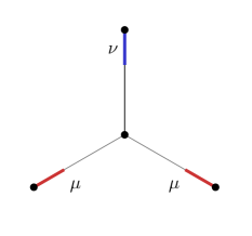
Figure 2. The support of probability measures $\mu$ and $\nu$ on a metric graph induced by a oriented star with 3 leaves

We impose an edge weight $1$ on each of the edges $e_{1},e_{2},f$. Consider the probability measures $\mu,\nu\in{\mathcal{P}}({\mathfrak{G}})$ with respective densities $\rho,\eta:{\mathfrak{G}}\to\mathbb{R}_{+}$ given by

$$\rho(x):=\begin{cases}\frac{1}{2\varepsilon}{\mathbbm{1}}_{[0,\varepsilon]}(x),&x\in e_{1}\text{ or }x\in e_{2},\\ 0,&x\in f,\end{cases},\quad\eta(x):=\begin{cases}0,&x\in e_{1}\text{ or }x\in e_{2},\\ \frac{1}{\varepsilon}{\mathbbm{1}}_{[1-\varepsilon,1]}(x),&x\in f.\end{cases}$$

Lemma 4.2.

The unique optimal coupling of $\mu$ and $\nu$ is given by monotone rearrangement from each of the edges $e_{1}$ and $e_{2}$ to $f$, i.e., by the map $T$ with

$$T(x)=1-\varepsilon+x\in f\qquad\text{ for }x\in e_{1}\text{ or }x\in e_{2}.$$

Proof.

Let $\pi$ be an optimal coupling of $\mu$ and $\nu$ and decompose it as $\pi=\pi_{1}+\pi_{2}$, where $\pi_{i}$, $i=1,2$, are couplings of $\mu_{i}$, the restriction of $\mu$ to $e_{i}$, and some $\nu_{i}$ a measure on $f$ such that $\nu_{1}+\nu_{2}=\nu$. Necessarily $\pi_{1},\pi_{2}$ are also optimal. By standard optimal transport theory on the interval $e_{i}\cup f\subset\mathbb{R}$, $\pi_{i}$ is given by a map $T_{i}$, the monotone rearrangement from $\mu_{i}$ to $\nu_{i}$. If we show that $\nu_{1}=\nu_{2}$, then $T_{1}=T_{2}=T$ with $T$ as above and the claim is proven. To this end, assume by contradiction that $\nu_{1}\neq\nu_{2}$ and hence $T_{1}\neq T_{2}$. We consider the coupling $\pi^{\prime}=\pi_{1}^{\prime}+\pi_{2}^{\prime}$ where $\pi_{1}^{\prime}=\pi_{2}^{\prime}=(\pi_{1}+\pi_{2})/2$ (here, we identify $e_{1}\cup f$ and $e_{2}\cup f$ in the obvious way). Since $T_{1}\neq T_{2}$, the support of $\pi_{1}^{\prime}$ is not contained in the graph of a function. Since $\pi^{\prime}$ is optimal, the couplings $\pi_{i}$ are also optimal between their marginals $\mu_{i}$ and $\frac{1}{2}\nu$, and thus have to be induced by the monotone rearrangement map $T$, a contradiction. ∎

Consequently, the constant speed-geodesic from $\mu$ to $\nu$ is thus given by $({T_{t}}_{\#}\mu)_{t\in[0,1]}$ where $T_{t}$ is the linear interpolation of $T$ and the identity on $e_{1}\cup f$ and $e_{2}\cup f$ respectively, more precisely

$$T_{t}(x):=\begin{cases}x+(2-\varepsilon)t\in e_{i},&\text{if }x\leq 1-(2-\varepsilon)t,\\ x+(2-\varepsilon)t-1\in f,&\text{if }x>1-(2-\varepsilon)t,\end{cases}$$

for $x\in e_{i}$, $i\in\{1,2\}$.

Set $t_{0}^{\varepsilon}:=\frac{1-\varepsilon}{2-\varepsilon}$ and $t_{1}^{\varepsilon}:=\frac{1}{2-\varepsilon}$. The relative entropy of $\mu_{t}$ is given by:

$$\operatorname{Ent}(\mu_{t})= \begin{cases}\log\bigl{(}\tfrac{1}{2\varepsilon}\bigr{)},&t\in[0,t_{0}^{\varepsilon}],\\ \frac{1}{\varepsilon}\big{(}1-(2-\varepsilon)t\big{)}\log\bigl{(}\tfrac{1}{2}\bigr{)}+\log\bigl{(}\frac{1}{\varepsilon}\bigr{)},&t\in[t_{0}^{\varepsilon},t_{1}^{\varepsilon}],\\ \log\bigr{(}\tfrac{1}{\varepsilon}\bigr{)},&\text{if }t\in[t_{1}^{\varepsilon},1].\end{cases}$$

Thus, $t\mapsto\operatorname{Ent}(\mu_{t})$ is piecewise affine; see Figure 3. It follows that $t\mapsto\operatorname{Ent}(\mu_{t})$ is not $\kappa$-convex for any $\kappa\in{\mathbb{R}}$.

Figure 3. Plot of the entropy along the geodesic interpolation

5. Gradient flows in the Wasserstein space over a metric graph

In this section we study gradient flows in the Wasserstein space over a metric graph. Namely, we consider diffusion equations on metric graphs arising as the gradient flow of free energy functionals composed as the sum of entropy, potential, and interaction energies. We give a variational characterisation of these diffusion equations via energy-dissipation identities and we discuss the approximation of solutions via the Jordan–Kinderlehrer–Otto scheme (minimizing movement scheme). This provides natural analogues on metric graphs of the corresponding classical results in Euclidean space. We follow the approach from the Euclidean case; see in particular [2, Section 10.4], and adapt it to the current setting.

Let $V:\overline{\mathfrak{E}}\to{\mathbb{R}}$ be Lipschitz continuous and define the weighted volume measure $\mathfrak{m}:=e^{-V}\lambda$ on ${\mathfrak{G}}$ (since $\lambda$ gives no mass to vertices, the potential ambiguity of $V$ there does not matter). We consider the following functionals on ${\mathcal{P}}({\mathfrak{G}})$:

1. the relative entropy ${\mathcal{E}}_{V}:{\mathcal{P}}({\mathfrak{G}})\to(-\infty,\infty]$ defined by

   $${\mathcal{E}}_{V}(\mu):={\rm Ent}[\mu|\mathfrak{m}]=\begin{cases}\int_{{\mathfrak{G}}}\rho(x)\log\rho(x)\,\mathrm{d}\mathfrak{m}(x)&\text{ if }\mu=\rho\mathfrak{m},\\ +\infty&\text{ otherwise}.\end{cases}$$ (5.1)

2. the interaction energy ${\mathcal{W}}:{\mathcal{P}}({\mathfrak{G}})\to\mathbb{R}$ defined by

   $${\mathcal{W}}(\mu):=\frac{1}{2}\int_{{\mathfrak{G}}\times{\mathfrak{G}}}W(x,y)\,\mathrm{d}\mu(x)\,\mathrm{d}\mu(y),$$

   where $W:{\mathfrak{G}}\times{\mathfrak{G}}\to\mathbb{R}$ is symmetric and Lipschitz continuous.

Moreover, we define ${\mathcal{F}}:{\mathcal{P}}({\mathfrak{G}})\to(-\infty,+\infty]$ as the sum of the previous quantities:

$${\mathcal{F}}:={\mathcal{E}}_{V}+{\mathcal{W}}.$$

Note that ${\mathcal{E}}_{V}$ is bounded from below (by Jensen’s inequality and finiteness of $\mathfrak{m}$) and lower semicontinuous with respect to weak convergence. Moreover, ${\mathcal{W}}$ is bounded and continuous with respect to weak convergence.

Further note that for $\mu\in{\mathcal{P}}({\mathfrak{G}})$ with $\mu\ll\lambda$ we can write

$${\mathcal{E}}_{V}(\mu)={\mathcal{E}}(\mu)+{\mathcal{V}}(\mu),$$

where ${\mathcal{E}}(\mu)={\rm Ent[\mu|\lambda]}$ is the Boltzmann entropy on ${\mathfrak{G}}$ and ${\mathcal{V}}:{\mathcal{P}}({\mathfrak{G}})\to\mathbb{R}$ defined by

$${\mathcal{V}}(\mu):=\int_{{\mathfrak{G}}}V(x)\,\mathrm{d}\mu(x)$$

is the potential energy. The latter is well defined for $\mu\ll\lambda$ despite the potential discontinuity of $V$ at the vertices.

5.1. Diffusion equation and energy dissipation

We consider the following diffusion equation on the metric graph ${\mathfrak{G}}$ given by

$$\partial_{t}\eta=\Delta\eta+\nabla\cdot\big{(}\eta\big{(}\nabla V+\nabla W[\mu]\big{)}\big{)}.$$ (5.2)

Here $\mu=\eta\lambda$ is a probability on $\mathfrak{G}$ and we set $W[\mu](x):=\int_{{\mathfrak{G}}}W(x,y)\,\mathrm{d}\mu(y)$. In analogy with the classical Euclidean setting we will show below that this PDE is the Wasserstein gradient flow equation of the free energy ${\mathcal{F}}$. Though the setting of metric graphs is one-dimensional, we prefer to use multi-dimensional notation such as $\Delta$ and $\nabla\cdot$ for the sake of clarity.

We consider the following notion of weak solution for (5.2).

Definition 5.1.

We say that a curve $(\eta_{t})_{t\in[0,T]}$ of probability densities w.r.t. $\lambda$ on ${\mathfrak{G}}$ is a weak solution to (5.2) if for $\rho_{t}:=\eta_{t}\cdot e^{V}$ we have $\rho_{t}\in W^{1,1}(\overline{{\mathfrak{E}}})\cap C({\mathfrak{G}})$ for a.e. $t$, and the pair $(\mu,J)$ given by

$$\mu_{t}=\rho_{t}\mathfrak{m}\quad\text{and}\quad J_{t}=-\left(\nabla\rho_{t}+\rho_{t}\nabla W[\mu_{t}]\right)\mathfrak{m}$$

is a weak solution to the continuity equation in the sense of Definition 3.2, i.e., we ask that $t\mapsto\mu_{t}$ is weakly continuous and for every $\varphi\in C^{1}_{c}\big{(}(0,T)\times\overline{\mathfrak{E}}\big{)}$ such that $\varphi_{t},\partial_{t}\varphi_{t}\in C^{1}(\overline{\mathfrak{E}})\cap C({{\mathfrak{G}}})$ for all $t\in(0,T)$, we have

$$\int_{0}^{T}\!\biggl{(}\int_{{\mathfrak{G}}}\partial_{t}\varphi\rho_{t}\,\mathrm{d}\mathfrak{m}-\int_{\overline{\mathfrak{E}}}\nabla\varphi\cdot\big{(}\nabla\rho_{t}+\rho_{t}\nabla W[\mu_{t}]\big{)}\,\mathrm{d}\mathfrak{m}\biggr{)}\,\mathrm{d}t=0.$$ (5.3)

Remark 5.2.

Let us briefly consider the special case where $V=W=0$. Then (5.2) is simply the heat equation on a metric graph, which has been introduced already in [18]. It is known since [15, 22] that the Laplacian with natural vertex conditions (continuity across the vertices along with a Kirchhoff-type condition on the fluxes) is associated with a Dirichlet form, hence the Cauchy problem for this PDE is well-posed on $L^{2}({\mathfrak{G}})$: more precisely, it is governed by an ultracontractive, Markovian $C_{0}$-semigroup $(\mathrm{e}^{t\Delta})_{t\geq 0}$ that extrapolates to $L^{p}({\mathfrak{G}})$ for all $p\geq 1$, as well as to $C({\mathfrak{G}})$ and, by duality, to the space $\mathcal{M}({\mathfrak{G}})$ of Radon measures on ${\mathfrak{G}}$. For any initial value $\mu_{0}\in{\mathcal{M}}({\mathfrak{G}})$, $(t,x)\mapsto\rho(t,x)=(\mathrm{e}^{t\Delta}\mu_{0})(x)$ defines a classical solution to the Cauchy problem for the heat equation with initial value $\mu_{0}$. It is easy to see that this solution is a weak solution in the sense of Definition 5.1 as well.

The dissipation of the free energy along solutions to (5.2) at $\mu=\rho\mathfrak{m}$ is formally given by

$$\frac{\mathrm{d}}{\mathrm{d}t}{\mathcal{F}}(\mu)=-\int_{{\mathfrak{E}}}\Big{|}\frac{\nabla\rho}{\rho}+\nabla W[\mu]\Big{|}^{2}\,\mathrm{d}\mu.$$

This motivates the following definition.

Definition 5.3 (Energy dissipation functional).

The energy dissipation functional ${\mathcal{I}}:{\mathcal{P}}({\mathfrak{G}})\to[0,+\infty]$ is defined as follows. If $\mu=\rho\mathfrak{m}$ with $\rho\in W^{1,1}(\overline{\mathfrak{E}})\cap C({\mathfrak{G}})$ and $\nabla\rho+\rho\nabla W[\mu]=\bm{w}\rho$ for some $\bm{w}\in L^{2}(\mu)$ we set

$${\mathcal{I}}(\mu):=\int_{{\mathfrak{E}}}|\bm{w}|^{2}\,\mathrm{d}\mu.$$

Otherwise, we set ${\mathcal{I}}(\mu)=+\infty$.

Remark 5.4.

We emphasize that continuity of $\rho$ on ${\mathfrak{G}}$ is required for finiteness of ${\mathcal{I}}(\mu)$ in this definition. It is not sufficient that $\rho$ belongs to $W^{1,1}(\overline{{\mathfrak{E}}})$. The continuity is important in the proof of Theorem 5.7 below, as it ensures spatial continuity for gradient flow curves (i.e., curves of maximal slope with respect to the upper gradient $\sqrt{{\mathcal{I}}}$) and it allows us to identify them with weak solutions to the diffusion equation (5.2). The requirement of spatial continuity for weak solutions to (5.2) in Definition 5.1 is essential in order to couple the dynamics on different edges across common vertices.

We collect the following properties of the dissipation functional.

Lemma 5.5.

Let $\{\mu_{n}\}_{n}\subseteq{\mathcal{P}}({\mathfrak{G}})$ be a sequence weakly converging to $\mu\in{\mathcal{P}}({\mathfrak{G}})$ such that

$$\sup_{n}\mathcal{F}(\mu_{n})<\infty\quad\text{and}\quad\sup_{n}{\mathcal{I}}(\mu_{n})<\infty.$$ (5.4)

Then we have

$$\mathcal{I}(\mu)\leq\liminf_{n}{\mathcal{I}}(\mu_{n}).$$ (5.5)

Proof.

First note that we can rewrite ${\mathcal{I}}(\mu)$ as the integral functional

$${\mathcal{I}}(\mu)=\mathcal{G}_{\alpha}(\mu,J)=\int_{{\mathfrak{E}}}\alpha\big{(}\frac{\mathrm{d}\mu}{\mathrm{d}\sigma},\frac{\mathrm{d}J}{\mathrm{d}\sigma}\big{)}\mathrm{d}\sigma,$$ (5.6)

where $\alpha:[0,\infty)\times\mathbb{R}\to[0,\infty]$ is the lower semicontinuous and convex function defined by

$$\alpha(s,u)=\begin{cases}|u|^{2}/s&\hbox{if }s>0,\\ 0&\hbox{if }s=0\hbox{ and }u=0,\\ +\infty&\text{otherwise},\end{cases}$$ (5.7)

and $J=\boldsymbol{w}\mu=(\nabla\rho+\rho\nabla W[\mu])\mathfrak{m}$. Here $\sigma$ is any measure such that $\mu,J\ll\sigma$; its choice is irrelevant by $1$-homogeneity of $\alpha$.

Now, let $\mu_{n}=\rho_{n}\mathfrak{m}$. Lower semicontinuity of ${\mathcal{F}}$ and (5.4) imply that ${\mathcal{F}}(\mu)<\infty$. Therefore we can write $\mu=\rho\mathfrak{m}$ for a suitable density $\rho$. Superlinearity of $r\mapsto r\log r$ implies that $\rho_{n}$ converges weakly to $\rho$ in $L^{1}({\mathfrak{G}},\mathfrak{m})$.

Recall that ${\mathcal{I}}(\mu_{n})=\int|\boldsymbol{w}_{n}|^{2}\mathrm{d}\mu_{n}$ with $U_{n}:=\rho_{n}\boldsymbol{w}_{n}=\nabla\rho_{n}+\rho_{n}\nabla W[\mu_{n}]$. Hölder’s inequality and the bound (5.4) yield that the measures $J_{n}=U_{n}\mathfrak{m}$ have uniformly bounded total variation. Hence up to extracting a subsequence, we have that $J_{n}$ converges weakly* to a measure $J$ on ${\mathfrak{E}}$. Lower semicontinuity of the integral functional $\mathcal{G}_{\alpha}$ yields

$$\mathcal{G}_{\alpha}(\mu,J)\leq\liminf_{n}{\mathcal{I}}(\mu_{n})<\infty.$$ (5.8)

This allows us to write $J=\boldsymbol{w}\rho\mathfrak{m}$ for a $\boldsymbol{w}\in L^{2}(\mu)$ and $\mathcal{G}_{\alpha}(\mu,J)=\int|\boldsymbol{w}|^{2}\mathrm{d}\mu$. Since $\rho_{n}\in W^{1,1}(\overline{\mathfrak{E}})\cap C({\mathfrak{G}})$, we have for any function $s\in C_{c}^{1}({\mathfrak{E}})$ by integration by parts,

$$-\int_{\mathfrak{G}}\rho_{n}\nabla s\,\mathrm{d}\lambda =\int_{\mathfrak{G}}s\nabla\rho_{n}\,\mathrm{d}\lambda$$ (5.9)

$$=\int_{\mathfrak{G}}se^{V}\big{(}\nabla\rho_{n}+\rho_{n}\nabla W[\mu_{n}]\big{)}\,\mathrm{d}\mathfrak{m}-\int_{{\mathfrak{G}}}se^{V}\nabla W[\mu_{n}]\,\mathrm{d}\mu_{n}$$

$$=\int_{\mathfrak{G}}se^{V}\,\mathrm{d}J_{n}-\int_{\mathfrak{G}}se^{V}\nabla W[\mu_{n}]\,\mathrm{d}\mu_{n}.$$

The convergence of $J_{n}$ to $J$ weakly and $\rho_{n}$ to $\rho$ in $L^{1}$ together with the fact that $J=\boldsymbol{w}\rho\mathfrak{m}$ gives no mass to $\sf V$ and the boundedness of $\nabla W$ allows us to pass to the limit and obtain

$$-\int_{\mathfrak{G}}\rho\nabla s\,\mathrm{d}\lambda=\int_{\mathfrak{G}}se^{V}\,\mathrm{d}J-\int_{\mathfrak{G}}se^{V}\nabla W[\mu]\,\mathrm{d}\mu=\int_{\mathfrak{G}}s\boldsymbol{w}\rho\,\mathrm{d}\lambda-\int_{\mathfrak{G}}s\rho\nabla W[\mu]\,\mathrm{d}\lambda$$

for all $s\in C_{c}^{1}({\mathfrak{E}})$. We infer that $\rho\in W^{1,1}(\overline{\mathfrak{E}})$ and that $\rho\boldsymbol{w}=\nabla\rho+\rho\nabla W[\mu]$. In particular, $\rho\in C(\overline{\mathfrak{E}})$ by the Sobolev embedding theorem.

Let us now show that $\rho\in C({\mathfrak{G}})$. For this purpose, note that each pair of adjacent edges $(e,f)$ can be identified with the interval $[-\ell_{e},\ell_{f}]$. Consider $s\in C^{1}({\mathfrak{E}})$ such that $s=0$ for all $g\neq e,f$ and $s=r$ on $e,f$ for some $r\in C_{c}^{1}(-\ell_{e},\ell_{f})$. Repeating the argument above, we infer that $\rho\in W^{1,1}([-\ell_{e},\ell_{f}])$ and in particular that $\rho$ is continuous at $0$. We thus obtain that $\rho\in C({\mathfrak{G}})$. Hence from (5.8) we obtain the claim. ∎

Let us denote by $\mathcal{I}_{0}$ the energy dissipation functional with $W=0$, more precisely, if $\mu=\rho\mathfrak{m}$ with $\rho\in W^{1,1}(\overline{\mathfrak{E}})\cap C({\mathfrak{G}})$ with $\nabla\rho=\bm{w}\rho$ for some $\bm{w}\in L^{2}(\mu)$ we set

$$\mathcal{I}_{0}(\mu):=\int_{\mathfrak{E}}|\bm{w}|^{2}\,\mathrm{d}\mu.$$

Otherwise, we set $\mathcal{I}_{0}(\mu)=+\infty$. Similarly as for ${\mathcal{I}}$ we can write ${\mathcal{I}}_{0}(\mu)=\int\alpha(\rho,\nabla\rho)\,\mathrm{d}\mathfrak{m}$ with $\mu=\rho\mathfrak{m}$ where $\alpha$ is the function in (5.7). Then $\mathcal{I}_{0}$ is a convex and lower semi-continuous functional by the previous lemma. We note that under the assumption that $W$ is Lipschitz, $\mathcal{I}(\mu)$ is finite if and only if $\mathcal{I}_{0}(\mu)$ is finite.

Next, we observe that finiteness of the $\mathcal{I}_{0}$ implies a quantitative $L^{\infty}$ bound on the density.

Lemma 5.6.

For $\mu\in{\mathcal{P}}({\mathfrak{G}})$ with ${\mathcal{I}}_{0}(\mu)<\infty$ and $\mu=\rho\mathfrak{m}$ we have $\rho\in C({\mathfrak{G}})$ with

$$\|\rho\|_{\infty}\leq A\sqrt{{\mathcal{I}}_{0}(\mu)},$$

where the constant $A>0$ depends on $\|V\|_{\infty}$.

Proof.

The continuity of $\rho$ follows from the definition of ${\mathcal{I}}_{0}(\mu)$. Using Hölder’s we obtain with $\nabla\rho=\rho\bm{w}$,

$$\int|\nabla\rho|\,\mathrm{d}\lambda \leq e^{\|V\|_{\infty}}\int|\nabla\rho|\,\mathrm{d}\mathfrak{m}\leq e^{\|V\|_{\infty}}\Big{(}\int|\bm{w}|^{2}\,\mathrm{d}\mu\Big{)}^{\frac{1}{2}}.$$

The claim then follows immediately from the Sobolev embedding theorem applied to each of the finitely many edges. ∎

5.2. Energy-dissipation equality

The main result of this section is the following gradient flow characterisation of the diffusion equation (5.2).

Theorem 5.7.

For any 2-absolutely continuous curve $(\mu_{t})_{t\in[0,T]}$ in $({\mathcal{P}}({\mathfrak{G}}),W_{2})$ with $\mathcal{F}(\mu_{0})<\infty$ we have

$$\mathcal{L}_{T}(\mu):=\mathcal{F}(\mu_{T})-\mathcal{F}(\mu_{0})+\frac{1}{2}\int_{0}^{T}{\left|\dot{\mu}\right|}^{2}(r)+{\mathcal{I}}(\mu_{r})\,\mathrm{d}r\geq 0.$$

Moreover, we have $\mathcal{L}_{T}(\mu)=0$ if and only if $\mu_{t}=\rho_{t}\mathfrak{m}$ is a weak solution to (5.2) in the sense of Definition 5.1.

The main step in proving this result is to establish a chain rule for the free energy $\mathcal{F}$ along absolutely continuous curves in $({\mathcal{P}}({\mathfrak{G}}),W_{2})$. Recall the definition of $\alpha$ from (5.7).

Proposition 5.8 (Chain rule).

Let $(\mu_{t})_{t\in[0,T]}$ be a $2$-absolutely continuous curve in $({\mathcal{P}}({\mathfrak{G}}),W_{2})$ satisfying $\int_{0}^{T}{\mathcal{I}}(\mu_{t})\,\mathrm{d}t<+\infty$. Write $\mu_{t}=\rho_{t}\mathfrak{m}$ and let $J_{t}=U_{t}\mathfrak{m}$ be an optimal family of momentum vector fields, i.e., $(\mu_{t},J_{t})_{t\in[0,T]}$ solves the continuity equation and $|\dot{\mu}|^{2}(t)=\int\alpha(\rho_{t},U_{t})\mathrm{d}\mathfrak{m}$. Let $\rho_{t}\bm{w}_{t}=\nabla\rho_{t}+\rho_{t}\nabla W[\mu_{t}]$ as in Definition 5.3. Then, $t\mapsto{\mathcal{F}}(\mu_{t})$ is absolutely continuous and we have

$$\frac{\,\mathrm{d}}{\,\mathrm{d}t}{\mathcal{F}}(\mu_{t})=\int_{\mathfrak{E}}\langle\bm{w_{t}},\mathrm{d}J_{t}\rangle\quad\text{ for a.e.~{}}t\in[0,T].$$ (5.10)

Proof.

We first note that the assumptions ensure that also $\int_{0}^{T}{\mathcal{I}}_{0}(\mu_{t})\,\mathrm{d}t<\infty$. Hence, we have

$$\int_{0}^{T}\int_{\mathfrak{E}}\alpha(\rho_{t},\nabla\rho_{t})\,\mathrm{d}\mathfrak{m}\,\mathrm{d}t<\infty,\qquad\int_{0}^{T}\int_{{\mathfrak{E}}}\alpha(\rho_{t},U_{t})\,\mathrm{d}\mathfrak{m}\,\mathrm{d}t<\infty.$$ (5.11)

We proceed by a twofold regularisation. Using a family $(\eta^{\delta})_{\delta>0}$ of even and smooth approximation kernels with compact support in $[-\delta,\delta]$, we regularise in time via

$$\rho^{\delta}_{t}:=\int_{-\delta}^{\delta}\eta^{\delta}(s)\rho_{t-s}\,\mathrm{d}s,$$

and set $\mu^{\delta}_{t}=\rho^{\delta}_{t}\mathfrak{m}$. Here we extend $\rho$ to a curve on the time-interval $[-\delta,T+\delta]$ which is constant on $[-\delta,0]$ and $[T,T+\delta]$. Similarly defining $J_{t}^{\delta}$ as the time-regularisation of $J_{t}$ we obtain that $(\mu^{\delta},J^{\delta})$ is a solution to the continuity equation. Convexity of ${\mathcal{I}}_{0}$ and the Benamou–Brenier functional yield that $\int_{0}^{T}{\mathcal{I}}_{0}(\mu^{\delta}_{t})\,\mathrm{d}t$ and $\int_{0}^{T}|\dot{\mu}^{\delta}|^{2}(t)\,\mathrm{d}t<\infty$. Hence, (5.11) also holds with $\rho^{\delta}_{t},U^{\delta}_{t}$ in place of $\rho_{t},U_{t}$. Moreover, we must have $U^{\delta}=0$ on $\{\rho^{\delta}=0\}$.

Further, we regularise the logarithm and define for $\varepsilon>0$ the function $F_{\varepsilon}:[0,\infty)\to\mathbb{R}$ by setting

$$F_{\varepsilon}(r)=(r+\varepsilon)\log(r+\varepsilon)-\varepsilon\log\varepsilon.$$

Then we define the regularized free energy ${\mathcal{F}}_{\varepsilon}$ of $\mu=\rho\mathfrak{m}$ via

$${\mathcal{F}}_{\varepsilon}(\mu)=\int_{{\mathfrak{G}}}F_{\varepsilon}(\rho)\,\mathrm{d}\mathfrak{m}+\frac{1}{2}\int_{{\mathfrak{G}}\times{\mathfrak{G}}}W(x,y)\,\mathrm{d}\mu(x)\,\mathrm{d}\mu(y).$$

Let us set $g^{\varepsilon,\delta}=F^{\prime}_{\varepsilon}(\rho^{\delta})=1+\log(\rho^{\delta}+\varepsilon)$. Note that by Lemma 5.6, $\rho_{\delta}$ is bounded and thus also $g^{\varepsilon,\delta}$ is bounded. We will first show that

$${\mathcal{F}}_{\varepsilon}(\mu^{\delta}_{T})-{\mathcal{F}}_{\varepsilon}(\mu^{\delta}_{0}) =\int_{0}^{T}\int_{{\mathfrak{G}}}\langle\nabla g^{\varepsilon,\delta}_{t}+\nabla W[\mu^{\delta}_{t}],\,\mathrm{d}J^{\delta}_{t}\rangle\,\mathrm{d}t.$$ (5.12)

Then passing to the limit $\delta,\varepsilon\to 0$ will yield the claim.

While establishing (5.12) we write $g$ instead of $g^{\varepsilon,\delta}$ for simplicity. We have

$${\mathcal{F}}_{\varepsilon}(\mu^{\delta}_{T})-{\mathcal{F}}_{\varepsilon}(\mu^{\delta}_{0}) =\int_{0}^{T}\int_{{\mathfrak{G}}}\big{(}F^{\prime}_{\varepsilon}(\rho^{\delta})+W[\mu^{\delta}_{t}]\big{)}\partial_{t}\rho^{\delta}_{t}\,\mathrm{d}\mathfrak{m}\,\mathrm{d}t.$$

Differentiation under the integral sign is justified by boundedness of $F^{\prime}_{\varepsilon}(\rho^{\delta})$ and $W$ and the regularity in time of $\rho^{\delta}$. Note that $W[\mu^{\delta}_{t}]$ is an admissible test function in the continuity equation for $(\mu^{\delta},J^{\delta})$. Thus, to establish (5.12) it remains to show that the continuity equation can also be used on the function $g=F^{\prime}_{\varepsilon}(\rho^{\delta})$. Recall that $g$ is bounded with $\nabla g=\nabla\rho^{\delta}/(\rho^{\delta}+\varepsilon)$. We can approximate $g$ uniformly by functions $g^{\alpha}\in C^{1}(\overline{\mathfrak{E}}\times[0,T])\cap C({\mathfrak{G}}\times[0,T])$ as follows. First extend $g$ to ${\mathfrak{G}}_{\rm ext}\times[0,T]$ with constant values on the additional edge incident to vertex $v$ equal to the value of $g$ at $v$. Then we apply the regularising procedure (3.10). The continuity equation for $(\mu^{\delta},J^{\delta})$ yields

$$\int_{0}^{T}\int_{{\mathfrak{G}}}g^{\alpha}_{t}\partial_{t}\rho^{\delta}_{t}\,\mathrm{d}\mathfrak{m}\,\mathrm{d}t=\int_{0}^{T}\int_{{\mathfrak{E}}}\langle\nabla g^{\alpha}_{t},\,\mathrm{d}J^{\delta}_{t}\rangle.$$

Passing to the limit as $\alpha\to 0$ then will finish the proof of (5.12). Convergence of the left hand side is immediate since $g$ is bounded and so $g^{\alpha}$ is bounded uniformly in $\alpha$. For the right hand side we estimate with $J^{\delta}=U^{\delta}\mathfrak{m}$:

$$\bigg{|}\int_{0}^{T}\int_{\mathfrak{E}}\langle\nabla g^{\alpha}_{t}-\nabla g_{t},\,\mathrm{d}J^{\delta}_{t}\rangle\,\mathrm{d}t\bigg{|} \leq\bigg{(}\int_{0}^{T}\int_{{\mathfrak{E}}}|\nabla g^{\alpha}_{t}-\nabla g_{t}|^{2}\rho^{\delta}_{t}\,\mathrm{d}\mathfrak{m}\,\mathrm{d}t\bigg{)}^{\frac{1}{2}}$$

$$\qquad\times\bigg{(}\int_{0}^{T}\int_{\mathfrak{E}}\alpha(\rho^{\delta}_{t},U^{\delta}_{t})\,\mathrm{d}\mathfrak{m}\,\mathrm{d}t\bigg{)}^{\frac{1}{2}}.$$

The second factor is finite as noted above. To estimate the first factor, we recall that $\rho^{\delta}$ is bounded. Hence for a suitable constant $C<\infty$

$$\int_{0}^{T}\int_{{\mathfrak{E}}}|\nabla g^{\alpha}_{t}-\nabla g_{t}|^{2}\rho^{\delta}_{t}\,\mathrm{d}\mathfrak{m}\,\mathrm{d}t\leq C\int_{0}^{T}\int_{{\mathfrak{E}}}|\nabla g^{\alpha}_{t}-\nabla g_{t}|^{2}\,\mathrm{d}\lambda\,\mathrm{d}t$$

Using (3.11) and dominated convergence, the latter term goes to zero as $\alpha\to 0$ if we show that

$$\int_{0}^{T}\int_{{\mathfrak{E}}}|\nabla g|^{2}\,\mathrm{d}\lambda\,\mathrm{d}t<\infty.$$

But using $\nabla g=\nabla\rho^{\delta}/(\rho^{\delta}+\varepsilon)$ we can estimate

$$\int_{0}^{T}\int_{{\mathfrak{E}}}|\nabla g|^{2}\,\mathrm{d}\lambda\,\mathrm{d}t \leq e^{\|V\|_{\infty}}\int_{0}^{T}{\mathcal{I}}_{0}(\mu\delta_{t})\,\mathrm{d}t<\infty.$$

Thus, (5.12) is established.

We will now pass to the limits $\delta,\varepsilon\to 0$ in (5.12), starting with the right-hand side.

For the limit $\delta\to 0$, note that $U^{\delta}\to U$ a.e. and $\boldsymbol{w}^{\varepsilon,\delta}\to\boldsymbol{w}^{\varepsilon}$ a.e. as $\delta\to 0$ with $\boldsymbol{w}^{\varepsilon}=\nabla\rho/(\rho+\varepsilon)+\nabla W[\mu]$. Dominated convergence then yields that as $\delta\to 0$:

$$\int_{0}^{T}\int_{{\mathfrak{E}}}\langle\boldsymbol{w}^{\varepsilon,\delta}_{t},U^{\delta}_{t}\rangle\,\mathrm{d}\mathfrak{m}\,\mathrm{d}t\rightarrow\int_{0}^{T}\int_{{\mathfrak{E}}}\langle\boldsymbol{w}^{\varepsilon}_{t},U_{t}\rangle\,\mathrm{d}\mathfrak{m}\,\mathrm{d}t.$$

Indeed, we have the majorant

$$|\langle\boldsymbol{w}^{\varepsilon,\delta},U^{\delta}\rangle| \leq\frac{1}{2}|\boldsymbol{w}^{\varepsilon,\delta}|^{2}(\rho^{\delta}+\varepsilon)+\frac{1}{2}\frac{|U^{\delta}|^{2}}{\rho^{\delta}+\varepsilon}\leq\alpha\big{(}\rho^{\delta},\nabla\rho^{\delta}\big{)}+C(\rho^{\delta}+\varepsilon)+\frac{1}{2}\alpha(\rho^{\delta},U^{\delta})$$

$$\leq\big{[}\alpha\big{(}\rho,\nabla\rho\big{)}\big{]}^{\delta}+C(\rho^{\delta}+\varepsilon)+\frac{1}{2}\big{[}\alpha(\rho,U)\big{]}^{\delta}$$

for a suitable constant $C$, using the fact $\nabla W[\rho^{\delta}]$ is uniformly bounded. Here, $\big{[}\cdot\big{]}^{\delta}$ denotes the time-regularisation of the function in brackets and we have used Jensen’s inequality in the last step to interchange the regularisation operation with the convex function $\alpha$. Since by assumption $\alpha\big{(}\rho,\nabla\rho\big{)}$ and $\alpha(\rho,U)$ are integrable on $[0,T]\times{\mathfrak{E}}$, the majorant above indeed converges in $L^{1}\big{(}[0,T]\times{\mathfrak{E}}\big{)}$.

To further pass to the limit $\varepsilon\to 0$, we note that $\boldsymbol{w}^{\varepsilon}\to\boldsymbol{w}$ a.e. on the set $\{\rho>0\}$. Since $U=0$ a.e. on the set $\{\rho=0\}$, we conclude that $\langle\boldsymbol{w}^{\varepsilon},U\rangle\to\langle\boldsymbol{w},U\rangle$ a.e. Using similar as before the majorant $|\langle\boldsymbol{w}^{\varepsilon},U\rangle|\leq\alpha\big{(}\rho,\nabla\rho\big{)}+C\rho+\alpha(\rho,U)/2$, we conclude by dominated convergence.

It remains to pass to the limit on the left-hand side in (5.12). The weak continuity of $t\mapsto\mu_{t}$ implies that $\mu^{\delta}_{t}\rightharpoonup\mu_{t}$ weakly as $\delta\to 0$. This is sufficient to conclude that $\mathcal{W}(\mu^{\delta}_{t})\to\mathcal{W}(\mu_{t})$. Note that for any $\mu=\rho\mathfrak{m}\in\mathcal{P}({\mathfrak{G}})$ we have

$$\int F_{\varepsilon}(\rho)\,\mathrm{d}\mathfrak{m}=\mathcal{E}_{V}(\mu^{\varepsilon})-M\varepsilon\log\varepsilon,$$

with $\mu^{\varepsilon}=(1+M)^{-1}(\mu+\varepsilon\mathfrak{m})$ and $M=\mathfrak{m}({\mathfrak{G}})$. Convexity of $r\mapsto r\log r$ and Jensen’s inequality yield that $\mathcal{E}_{V}(\mu^{\delta,\varepsilon}_{t})\leq\mathcal{E}_{V}(\mu^{\varepsilon}_{t})$. Thus, lower semicontinuity of $\mathcal{E}_{V}$ under weak convergence shows that $\mathcal{E}_{V}(\mu^{\delta,\varepsilon}_{t})\to\mathcal{E}_{V}(\mu^{\varepsilon}_{t})$ and hence $\int F_{\varepsilon}(\rho^{\delta}_{t})\,\mathrm{d}\mathfrak{m}\to\int F_{\varepsilon}(\rho_{t})\,\mathrm{d}\mathfrak{m}$ as $\delta\to 0$. The limit $\varepsilon\to 0$ is then easily achieved by monotone convergence. From the convergence of the right-hand side of (5.12) and the assumption that ${\mathcal{F}}(\mu_{0})<\infty$ we finally conclude that ${\mathcal{F}}(\mu_{t})<\infty$ for all $t>0$ and that

$${\mathcal{F}}(\mu_{T})-{\mathcal{F}}(\mu_{0})=\int_{0}^{T}\int\langle\boldsymbol{w}_{t},\,\mathrm{d}J_{t}\rangle\,\mathrm{d}t.$$

Hence $t\mapsto{\mathcal{F}}(\mu_{t})$ is absolutely continuous and (5.10) follows. ∎

We can now prove Theorem 5.7.

Proof of Theorem 5.7.

Note that the right-hand side of (5.10) may be estimated by means of Hölder’s and Young’s inequality as

$$\int_{\mathfrak{E}}\langle\bm{w}_{t},U_{t}\rangle\,\mathrm{d}\mathfrak{m}\geq-\sqrt{\int_{{\mathfrak{E}}}{\left|\bm{w}_{t}\right|}^{2}\rho_{t}\,\mathrm{d}\mathfrak{m}}\sqrt{\int_{{\mathfrak{E}}}\frac{{\left|U_{t}\right|}^{2}}{\rho_{t}}\,\mathrm{d}\mathfrak{m}}\geq-\frac{1}{2}\int_{\mathfrak{E}}{\left|\bm{w}_{t}\right|}^{2}\rho_{t}\,\mathrm{d}\mathfrak{m}-\frac{1}{2}\int_{{\mathfrak{E}}}\frac{{\left|U_{t}\right|}^{2}}{\rho_{t}}\,\mathrm{d}\mathfrak{m}.$$ (5.13)

Hence, by integrating both sides of (5.10) from $0$ to $T$ we obtain that $\mathcal{L}_{T}(\mu)\geq 0$. Moreover, we have equality if and only if for a.e. $t$ and $\mu_{t}$-a.e. we have $U_{t}=-\rho_{t}\bm{w}_{t}$. Now the continuity equation with $J_{t}=U_{t}\mathfrak{m}=-\rho_{t}\bm{w}_{t}\mathfrak{m}=-\nabla\rho_{t}+\rho_{t}\nabla W[\mu_{t}]\mathfrak{m}$ becomes the weak formulation of (5.2) ∎

5.3. Metric gradient flows

Here, we recast the variational characterisation of McKean–Vlasov equations on metric graphs from the previous section in the language of the theory of gradient flows in metric spaces. Let us briefly recall the basic objects. For a detailed account we refer the reader to [2].

Let $(X,d)$ be a complete metric space and let $E:X\to(-\infty,\infty]$ be a function with proper domain, i.e., the set $D(E):=\{x:E(x)<\infty\}$ is non-empty.

The following notion plays the role of the modulus of the gradient in a metric setting.

Definition 5.9 (Strong upper gradient).

A function $g:X\to[0,\infty]$ is called a strong upper gradient of $E$ if for any $x\in AC\big{(}(a,b);(X,d)\big{)}$ the function $g\circ x$ is Borel and

$$|E(x_{s})-E(x_{t})|~{}\leq~{}\int_{s}^{t}g(x_{r})|\dot{x}|(r)\,\mathrm{d}r\quad\forall~{}a\leq s\leq t\leq b\ .$$

Note that by the definition of strong upper gradient, and Young’s inequality $ab\leq\frac{1}{2}(a^{2}+b^{2})$, we have that for all $s\leq t$:

$$E(x_{t})-E(x_{s})+\frac{1}{2}\int_{s}^{t}g(x_{r})^{2}+|\dot{x}|^{2}(r)\,\mathrm{d}r\geq 0.$$

Definition 5.10 (Curve of maximal slope).

A locally $2$-absolutely continuous curve $(x_{t})_{t\in(0,\infty)}$ is called a curve of maximal slope of $E$ with respect to its strong upper gradient $g$ if $t\mapsto E(x_{t})$ is non-increasing and

$$E(x_{t})-E(x_{s})+\frac{1}{2}\int_{s}^{t}g(x_{r})^{2}+|\dot{x}|^{2}(r)\,\mathrm{d}r\leq 0\quad\forall~{}0<s\leq t.$$ (5.14)

We say that a curve of maximal slope starts from $x_{0}\in X$ if $\lim_{t\searrow 0}x_{t}=x_{0}$.

Equivalently, we can require equality in (5.14). If a strong upper gradient $g$ of $E$ is fixed we also call a curve of maximal slope of $E$ (relative to $g$) a gradient flow curve.

Finally, we define the (descending) metric slope of $E$ as the function $|\partial E|:D(E)\to[0,\infty]$ given by

$$|\partial E|(x)=\limsup_{y\to x}\frac{\max\{E(x)-E(y),0\}}{d(x,y)}.$$ (5.15)

The metric slope is in general only a weak upper gradient for $E$, see [2, Theorem 1.2.5]. In our application to metric graphs we will show that the square root of the dissipation ${\mathcal{I}}$ provides a strong upper gradient for the free energy ${\mathcal{F}}$.

Corollary 5.11.

The functional $\sqrt{{\mathcal{I}}}$ is a strong upper gradient of ${\mathcal{F}}$ on $({\mathcal{P}}({\mathfrak{G}}),W_{2})$. The curves of maximal slope for ${\mathcal{F}}$ with respect to this strong upper gradient coincide with weak solutions to (5.2) satisfying $\int_{0}^{T}{\mathcal{I}}(\mu_{t})\,\mathrm{d}t<\infty$.

Proof.

For a $2$-absolutely continuous curve with $(\mu_{t})_{t}$ with $\int_{0}^{T}{\mathcal{I}}(\mu_{t})\,\mathrm{d}t<\infty$, the chain rule (5.10) together with the estimate (5.13) yields

$${\left|{\mathcal{F}}(\mu_{t})-{\mathcal{F}}(\mu_{s})\right|}\leq\int_{s}^{t}\sqrt{{\mathcal{I}}(\mu_{r})}{\left|\dot{\mu}_{r}\right|}\,\mathrm{d}r\qquad\forall s,t\in[0,T]:s\leq t,$$ (5.16)

i.e., $\sqrt{{\mathcal{I}}}$ is a strong upper gradient. Theorem 5.7 yields the identification of curves of maximal slope. ∎

The dissipation functional ${\mathcal{I}}(\mu)$ can be related to the metric slope of the free energy ${\mathcal{F}}$ under suitable conditions on $\mu\in{\mathcal{P}}({\mathfrak{G}})$.

Lemma 5.12.

For any $\mu\in{\mathcal{P}}({\mathfrak{G}})$ we have

$${\mathcal{I}}(\mu)\leq{\left|\partial{\mathcal{F}}\right|}^{2}(\mu).$$

Proof.

We assume that $\mu=\rho\mathfrak{m}=\tilde{\rho}\lambda\in{\mathcal{P}}({\mathfrak{G}})$ satisfies ${\left|\partial\mathcal{F}\right|}(\mu)<\infty$, since otherwise there is nothing to prove.

Step 1. We show first that $\rho\in W^{1,1}(\overline{\mathfrak{E}})$ and $\nabla\rho+\rho\nabla W[\mu]=\rho\boldsymbol{w}$ with $\boldsymbol{w}\in L^{2}(\mu)$.

For this purpose, take any $\boldsymbol{s}\in C^{\infty}(\overline{{\mathfrak{E}}})$ which vanishes in a neighbourhood of every node and put $\tilde{\boldsymbol{s}}=e^{V}\boldsymbol{s}$. As a consequence, the mapping $r_{t}:{\mathfrak{G}}\to{\mathfrak{G}}$ defined by $r_{t}:={\operatorname{Id}}+t\tilde{\boldsymbol{s}}$ maps each edge into itself for $t>0$ sufficiently small. We claim that:

$$\lim_{t\searrow 0}\frac{\mathcal{F}\big{(}(\boldsymbol{r}_{t})_{\#}\mu\big{)}-\mathcal{F}(\mu)}{t}=\int_{\mathfrak{G}}\big{[}-\rho\nabla\boldsymbol{s}+\boldsymbol{s}\rho\nabla W[\mu]\big{]}\,\mathrm{d}\lambda.$$ (5.17)

To show this, note that $\boldsymbol{r}_{t}$ is injective for every $t$ small enough. Therefore, the change of variables formula yields that the density $\tilde{\rho}_{t}$ of $(\boldsymbol{r}_{t})_{\#}\mu$ with respect to $\lambda$ satisfies

$$\tilde{\rho}(x)=\tilde{\rho}_{t}(\boldsymbol{r}_{t}(x))\nabla\boldsymbol{r}_{t}(x).$$

Consequently, with $F(r)=r\log r$ we have

$$\mathcal{F}((\boldsymbol{r}_{t})_{\#}\mu)-\mathcal{F}(\mu)= \int_{\mathfrak{G}}F\Bigl{(}\frac{\tilde{\rho}}{\nabla\boldsymbol{r}_{t}}\Bigr{)}\nabla\boldsymbol{r}_{t}-F(\tilde{\rho})\,\mathrm{d}\lambda+\int_{\mathfrak{G}}[V\circ\boldsymbol{r}_{t}-V]\,\mathrm{d}\mu$$

$$+\int_{{\mathfrak{G}}\times{\mathfrak{G}}}[W\circ(\boldsymbol{r}_{t}\otimes\boldsymbol{r}_{t})-W]\,\mathrm{d}\mu\otimes\mu.$$

Note that $\nabla\boldsymbol{r}_{t}=1+t\nabla\tilde{\boldsymbol{s}}$. Dividing by $t$ and letting $t\searrow 0$ and noting that $\nabla\tilde{\boldsymbol{s}}=e^{V}(\nabla\boldsymbol{s}+\boldsymbol{s}\nabla V)$ and $\tilde{\rho}\tilde{\boldsymbol{s}}=\rho\boldsymbol{s}$ we deduce (5.17).

For $t>0$ sufficiently small, we then have

$$W_{2}\big{(}\mu,(\boldsymbol{r}_{t})_{\#}\mu\big{)}\leq t{\left\|\tilde{\boldsymbol{s}}\right\|}_{L^{2}(\mu)}.$$

This estimate, together with (5.17), implies

$$\int_{\mathfrak{G}}\big{[}-\rho\nabla\boldsymbol{s}+\boldsymbol{s}\rho\nabla W[\mu]\big{]}\,\mathrm{d}\lambda=\lim_{t\searrow 0}\frac{\mathcal{F}\big{(}(\boldsymbol{r}_{t})_{\#}\mu\big{)}-\mathcal{F}(\mu)}{t}\leq{\left|\partial\mathcal{F}\right|}(\mu){\left\|\tilde{\boldsymbol{s}}\right\|}_{L^{2}(\mu)}.$$

Hence, the left-hand side defines an $L^{2}(\mu)$-bounded linear functional on a subspace of $L^{2}(\mu)$. Using the Hahn–Banach theorem we may extend this functional to $L^{2}(\mu)$. The Riesz representation theorem then yields a unique element $\bm{w}\in L^{2}(\mu)$ such that ${\left\|\bm{w}\right\|}_{L^{2}(\mu)}\leq{\left|\partial\mathcal{F}\right|}(\mu)$ and

$$\int_{\mathfrak{G}}\big{[}-\rho\nabla\boldsymbol{s}+\boldsymbol{s}\rho\nabla(V+W[\mu])\big{]}\,\mathrm{d}\lambda=\int_{\mathfrak{G}}\boldsymbol{w}\tilde{\boldsymbol{s}}\,\mathrm{d}\mu=\int_{\mathfrak{G}}\boldsymbol{w}\rho s\,\mathrm{d}\lambda$$ (5.18)

for all $\boldsymbol{s}$ as above.

Considering in particular functions $\boldsymbol{s}$ supported on a single edge, we infer that $\rho\in W^{1,1}(\overline{\mathfrak{E}})$ and $\nabla\rho+\rho\nabla W[\mu]=\rho\boldsymbol{w}$ with $\boldsymbol{w}\in L^{2}(\mu)$. In particular, we have $\rho\in C(\overline{\mathfrak{E}})$ by Sobolev embedding.

Step 2. Next we show that $\rho$ belongs to $C({\mathfrak{G}})$. For this purpose we repeat the argument above, for a different class of functions $\boldsymbol{s}$.

Consider a pair of adjacent edges $e,f\in\mathsf{E}$ with common vertex $v$. For the moment, we identify the concatenation of the two edges with the interval $[-\ell_{e},\ell_{f}]$ such that $v$ corresponds to $0$. Let $s:[-\ell_{e},\ell_{f}]\to\mathbb{R}$ be a $C^{\infty}$-function vanishing in a neighbourhood of $-\ell_{e}$ and $\ell_{f}$. In particular, $r_{t}:={\operatorname{Id}}+t\tilde{s}$ maps $[-\ell_{e},\ell_{f}]$ into itself for $t>0$ sufficiently small, where $\tilde{s}=e^{V}s$. Let the maps $\boldsymbol{s}:{\mathfrak{E}}\to\mathbb{R}$ and ${\mathbf{r}}_{t}:{\mathfrak{E}}\to{\mathfrak{G}}$ be defined on $e\cup f$ by $s$ and $r_{t}$ through the identification with $[-\ell_{e},\ell_{f}]$ and by setting $\boldsymbol{s}=0$ and ${\mathbf{r}}_{t}={\rm id}$ on all other edges. Repeating the argument from Step 1, we infer that $\rho\in W^{1,1}([-\ell_{e},\ell_{f}])$ with the identification of $e,f$ with $[-\ell_{e},\ell_{f}]$ as above. In particular, $\rho$ is continuous at $0$. Since the choice of the pair $e,f$ is arbitrary, we conclude that $\rho\in C({\mathfrak{G}})$.

Combining both steps, we infer that ${\mathcal{I}}(\mu)<\infty$ and

$${\mathcal{I}}(\mu)=\|\boldsymbol{w}\|_{L^{2}(\mu)}^{2}\leq{\left|\partial{\mathcal{F}}\right|}^{2}(\mu).$$

∎

From Lemma 5.12 and the lower semicontinuity of $\mathcal{I}$ we immediately infer that $\sqrt{{\mathcal{I}}}$ lies below the relaxed metric slope, i.e., the lower semicontinuous relaxation of $|\partial\mathcal{F}|$ given by

$$|\partial^{-}\mathcal{F}|(\mu):=\inf\big{\{}\liminf_{n}|\partial\mathcal{F}|(\mu_{n})~{}:~{}\mu_{n}\rightharpoonup\mu\big{\}}.$$

Corollary 5.13.

For all $\mu\in{\mathcal{P}}({\mathfrak{G}})$ we have $\sqrt{{\mathcal{I}}(\mu)}\leq|\partial^{-}\mathcal{F}|(\mu)$.

5.4. Approximation via the JKO scheme

In this section, we consider the time-discrete variational approximation scheme of Jordan–Kinderlehrer–Otto for the gradient flow [14].

Given a time step $\tau>0$ and an initial datum $\mu_{0}\in{\mathcal{P}}({\mathfrak{G}})$ with $\mathcal{F}(\mu_{0})<\infty$, we consider a sequence $(\mu^{\tau}_{n})_{n}$ in ${\mathcal{P}}({\mathfrak{G}})$ defined recursively via

$$\mu^{\tau}_{0}=\mu_{0},\quad\mu^{\tau}_{n}\in\underset{\nu}{\operatorname*{argmin}}\Big{\{}\mathcal{F}(\nu)+\frac{1}{2\tau}W_{2}(\nu,\mu^{\tau}_{n-1})^{2}\Big{\}}.$$ (5.19)

Then we build a discrete gradient flow trajectory as the piecewise constant interpolation $(\bar{\mu}^{\tau}_{t})_{t\geq 0}$ given by

$$\bar{\mu}^{\tau}_{0}=\mu_{0},\quad\bar{\mu}^{\tau}_{t}=\mu^{\tau}_{n}\ \text{if }t\in\big{(}(n-1)\tau,n\tau].$$ (5.20)

Then we have the following result.

Theorem 5.14.

For any $\tau>0$ and $\mu_{0}\in{\mathcal{P}}({\mathfrak{G}})$ with $\mathcal{F}(\mu_{0})<\infty$ the variational scheme (5.19) admits a solution $(\mu^{\tau}_{n})_{n}$. As $\tau\to 0$, for any family of discrete solutions there exists a sequence $\tau_{k}\to 0$ and a locally $2$-absolutely continuous curve $(\mu_{t})_{t\geq 0}$ such that

$$\bar{\mu}^{\tau_{k}}_{t}\rightharpoonup\mu_{t}\quad\forall t\in[0,\infty).$$ (5.21)

Moreover, any such limit curve is a gradient flow curve of $\mathcal{F}$, i.e., a weak solution to the diffusion equation (5.2).

Proof of Theorem 5.14.

The result basically follows from general results for metric gradient flows, where the scheme is known as the minimizing movement scheme; see [2, Section 2.3]. We consider the metric space $({\mathcal{P}}({\mathfrak{G}}),W_{2})$ and endow it with the weak topology $\sigma$. It follows that [2, Assumptions 2.1 (a,b,c)] are satisfied. Existence of a solution to the variational scheme (5.19) and of a subsequential limit curve $(\mu_{t})_{t}$ now follows from [2, Corollary 2.2.2, Proposition 2.2.3]. Moreover, [2, Theorem 2.3.2] gives that the limit curve is a curve of maximal slope for the strong upper gradient $|\partial^{-}\mathcal{F}|$, i.e.,

$$\frac{1}{2}\int_{0}^{t}|\dot{\mu}|^{2}(r)+|\partial^{-}\mathcal{F}(\mu_{r})|^{2}\,\mathrm{d}r+\mathcal{F}(\mu_{t})\leq\mathcal{F}(\mu_{0}).$$

Thus, by Corollary 5.13, it is also a curve of maximal slope for the strong upper gradient $\sqrt{{\mathcal{I}}}$. Theorem 5.7 yields the identification with weak solutions to (5.2). ∎

Acknowledgement

ME acknowledges funding by the Deutsche Forschungsgemeinschaft (DFG), Grant SFB 1283/2 2021 – 317210226. DF and JM were supported by the European Research Council (ERC) under the European Union’s Horizon 2020 research and innovation programme (grant agreement No 716117). JM also acknowledges support by the Austrian Science Fund (FWF), Project SFB F65. The work of DM was partially supported by the Deutsche Forschungsgemeinschaft (DFG), Grant 397230547. This article is based upon work from COST Action 18232 MAT-DYN-NET, supported by COST (European Cooperation in Science and Technology), www.cost.eu. We wish to thank Martin Burger and Jan-Frederik Pietschmann for useful discussions. We are grateful to the anonymous referees for their careful reading and useful suggestions.

References

• [1] L. Ambrosio and N. Gigli. A user’s guide to optimal transport. In Modelling and optimisation of flows on networks, pages 1–155. Springer, 2013.
• [2] L. Ambrosio, N. Gigli, and G. Savaré. Gradient flows: in metric spaces and in the space of probability measures. Springer Science & Business Media, 2008.
• [3] L. Ambrosio, N. Gigli, and G. Savaré. Calculus and heat flow in metric measure spaces and applications to spaces with Ricci bounds from below. Inventiones mathematicae, 195(2):289–391, 2014.
• [4] J.-D. Benamou and Y. Brenier. A numerical method for the optimal time-continuous mass transport problem and related problems. Contemporary Mathematics, 226:1–12, 1999.
• [5] J.-D. Benamou and Y. Brenier. A computational fluid mechanics solution to the Monge-Kantorovich mass transfer problem. Numerische Mathematik, 84(3):375–393, 2000.
• [6] G. Berkolaiko and P. Kuchment. Introduction to Quantum Graphs, volume 186 of Math. Surveys and Monographs. Amer. Math. Soc., Providence, RI, 2013.
• [7] M. Bernot, V. Caselles, and J.-M. Morel. Optimal transportation networks, volume 1955 of Lecture Notes in Mathematics. Springer-Verlag, Berlin, 2009. Models and theory.
• [8] V. I. Bogachev. Measure theory, volume 1. Springer Science & Business Media, 2007.
• [9] D. Burago, Y. Burago, and S. Ivanov. A Course in Metric Geometry, volume 33 of Graduate Studies in Mathematics. Amer. Math. Soc., Providence, RI, 2001.
• [10] M. Burger, I. Humpert, and J.-F. Pietschmann. Dynamic optimal transport on networks. arXiv:2101.03415, 2021.
• [11] S.-N. Chow, W. Huang, Y. Li, and H. Zhou. Fokker-Planck equations for a free energy functional or Markov process on a graph. Arch. Ration. Mech. Anal., 203(3):969–1008, 2012.
• [12] D. Cordero-Erausquin, R. J. McCann, and M. Schmuckenschläger. A Riemannian interpolation inequality à la Borell, Brascamp and Lieb. Invent. Math., 146(2):219–257, 2001.
• [13] N. Gigli and B.-X. Han. The continuity equation on metric measure spaces. Calculus of Variations and Partial Differential Equations, 53(1-2):149–177, 2015.
• [14] R. Jordan, D. Kinderlehrer, and F. Otto. The variational formulation of the Fokker–Planck equation. SIAM Journal on Mathematical Analysis, 29(1):1–17, 1998.
• [15] M. Kramar Fijavž, D. Mugnolo, and E. Sikolya. Variational and semigroup methods for waves and diffusion in networks. Appl. Math. Optim., 55:219–240, 2007.
• [16] P. Kuchment. Quantum graphs: an introduction and a brief survey. In Analysis on graphs and its applications, volume 77 of Proc. Sympos. Pure Math., pages 291–312. Amer. Math. Soc., Providence, RI, 2008.
• [17] M. Liero, A. Mielke, and G. Savaré. Optimal entropy-transport problems and a new Hellinger-Kantorovich distance between positive measures. Invent. Math., 211(3):969–1117, 2018.
• [18] G. Lumer. Connecting of local operators and evolution equations on networks. In F. Hirsch, editor, Potential Theory (Proc. Copenhagen 1979), pages 230–243, Berlin, 1980. Springer-Verlag.
• [19] J. Maas. Gradient flows of the entropy for finite Markov chains. J. Funct. Anal., 261(8):2250–2292, 2011.
• [20] J. M. Mazón, J. D. Rossi, and J. Toledo. Optimal mass transport on metric graphs. SIAM J. Optim., 25(3):1609–1632, 2015.
• [21] A. Mielke. A gradient structure for reaction-diffusion systems and for energy-drift-diffusion systems. Nonlinearity, 24(4):1329–1346, 2011.
• [22] D. Mugnolo. Gaussian estimates for a heat equation on a network. Networks Het. Media, 2:55–79, 2007.
• [23] D. Mugnolo. Semigroup methods for evolution equations on networks. Understanding Complex Systems. Springer, Cham, 2014.
• [24] F. Otto and C. Villani. Generalization of an inequality by Talagrand and links with the logarithmic Sobolev inequality. J. Funct. Anal., 173(2):361–400, 2000.
• [25] M.-K. v. Renesse and K.-T. Sturm. Transport inequalities, gradient estimates, entropy, and Ricci curvature. Comm. Pure Appl. Math., 58(7):923–940, 2005.
• [26] F. Santambrogio. Optimal transport for applied mathematicians, volume 55 of Progress in Nonlinear Differential Equations and Their Applications. Birkhäuser, Cham, 2015.
• [27] C. Villani. Optimal transport: old and new, volume 338. Springer Science & Business Media, 2008.
• [28] Q. Xia. Optimal paths related to transport problems. Commun. Contemp. Math., 5(2):251–279, 2003.