Heat fluctuations in the logarithm-harmonic potential

Abstract

Thermodynamic quantities, like heat, entropy, or work, are random variables, in stochastic systems. Here, we investigate the statistics of the heat exchanged by a Brownian particle subjected to a logarithm-harmonic potential. We derive analytically the characteristic function and its moments for the heat. Through numerical integration, and numerical simulation, we calculate the probability distribution as well, characterizing fully the statistical behavior of the heat. The results are also investigated in the asymptotic limit, where we encounter the characteristic function in terms of hypergeometric functions.

Keywords: heat fluctuations; stochastic thermodynamics; exact results.

I Introduction

Diffusive systems such as Brownian particles exist in mesoscopic scales, ranging from a few nano-meters to micro-meters, where thermal fluctuations play an important role. In general, these systems are far away from equilibrium, and their thermodynamic quantities, like heat, or work, become random variables. In order to describe the thermodynamics of mesoscopic systems, we can use the Stochastic Thermodynamic framework oliveira2020classical ; ciliberto_experiments_2017 ; seifert2012stochastic ; sekimoto2010stochastic . In this framework, thermodynamic quantities become stochastic, having an associated probability distribution. This can be contrasted to the usual thermodynamic quantities which have negligible fluctuations due to thermodynamic limit.

Characterization of the statistics of the thermodynamic quantities of diffusive systems was carried in many different models. Derivations of the distribution and characteristic function for work and heat had been solved for Brownian systems, ranging from the free particle to non-harmonic potentials with theoretical paraguassu_heat_2021 ; chatterjee_exact_2010 ; chatterjee_single-molecule_2011 ; ghosal_distribution_2016 ; saha_work_2014 ; kusmierz_heat_2014 ; chvosta_statistics_2020 ; goswami_heat_2019 ; goswami_work_2019 ; goswami_work_2021 ; kwon_work_2013 ; jimenez-aquino_thermodynamic_2018 and experimental joubaud_fluctuation_2007 ; gomez-solano_heat_2011 ; imparato_work_2007 ; imparato_probability_2008 results. These works bring physical insights in the thermodynamics of such systems. In particular, we are interested in investigating the fluctuations of heat in a diffusive system with logarithm-harmonic potential. The fluctuations can be understood by the probability distribution or the characteristic function. The later is more easily derived, however, the distribution is also desired, since allows us a direct interpretation of its behavior through a more simple visualization. The physical picture we have in mind is that of an electrolyte interacting with a charged polymer by means of an electric interaction and a harmonic potential.

Concerning the logarithm potential, the heat distribution for the case without the harmonic term was already studied by the authors in paraguassu_heat_2021 . Moreover, the work for in the logarithm harmonic system was studied in ryabov_work_2013 ; holubec_asymptotics_2015 ; ryabov2015stochastic , where the time-variation of the stiffness of the harmonic term allows us to extract work from the particle. While the work properties was already investigated in ryabov_work_2013 ; holubec_asymptotics_2015 ; ryabov2015stochastic , the heat distribution is still not studied, asfar as we know. Hence, we present herein a comprehensible investigation of the heat distribution, obtaining its probability and characteristic function.

Diffusive systems under a Logarithm potential have stirred some interest in the literature leibovich_aging_2016 ; hirschberg_approach_2011 ; aghion_non-normalizable_2019 ; dechant_superaging_2012 ; barkai_area_2014 ; kessler_infinite_2010 ; ray_diffusion_2020 due to its intriguing effects, such as ergodicity breaking dechant_superaging_2012 , anomalous diffusion barkai_area_2014 ; kessler_infinite_2010 , and resetting phenomena ray_diffusion_2020 , to name but a few. Moreover, the logarithm potential can represent different systems bray_random_2000 ; ryabov_brownian_2015 ; fogedby_dna_2007 ; lo_dynamics_2002 ; campisi_logarithmic_2012 ; kessler_infinite_2010 ; barkai_area_2014 . Regarding the Brownian particle, the logarithm potential can represent the Coulomb force of a line of charges manning_limiting_1969 ; liboff_brownian_1966 , which is used to model a long polymer interacting with a charged Brownian particle manning_limiting_1969 . In our case, in addition we have a harmonic potential, which can represent an asymmetric trap potential ryabov2015stochastic allowing us to have a defined equilibrium distribution.

In stochastic thermodynamics, heat is in a sense a more fundamental quantity than work. Since, to exchange work with an external system, it is necessary that the system interact with the external system in an ordered way. Conversely, the heat will always be present since it is the energy exchanged between the particle and the heat bath sekimoto2010stochastic in a disordered, and spontaneous, way. Nevertheless, because of its definition, heat cannot be measured directly for a Brownian system. An alternative is to measure the trajectories and then construct the statistics of the heat ciliberto_experiments_2017 . Therefore, a theoretical investigation is always desired to compare with experimental results. Theoretical heat distributions results can be found in paraguassu_heat_2021_2 ; paraguassu_heat_2021 ; gupta_heat_2021 ; fogedby_heat_2020 ; goswami_heat_2019 ; crisanti_heat_2017 ; ghosal_distribution_2016 ; rosinberg_heat_2016 ; kim_heat_2014 ; kusmierz_heat_2014 ; saha_work_2014 ; chatterjee_single-molecule_2011 ; chatterjee_exact_2010 ; fogedby_heat_2009 ; imparato_probability_2008 ; imparato_work_2007 ; joubaud_fluctuation_2007 . Here, combining analytical methods with numerical simulations we derived the heat distribution for the logarithm-harmonic potential, extending the list of results in heat distributions.

The present paper is organized as follows: In section 2 we describe the dynamics and thermodynamics of the Brownian particle in a logarithm-harmonic potential. In section 3 we derive the probability distribution of the heat. In section 4 we analyze the characteristic function and calculate the moments of the distribution. In section 5 we give the details of the numeric simulation. We finish in section 6 with the discussion of the results and the conclusion.

II Stochastic Thermodynamics and Dynamics of the particle

In this paper, we consider a diffusive particle, in the overdamped limit, under a logarithm and a harmonic potential. The logarithm potential can represent the potential of a line of charge, while the harmonic potential is often used to model the action of optical tweezers. Together, the potentials can represent an asymmetric trap. Here, following bray_random_2000 ; ryabov_work_2013 ; giampaoli_exact_1999 we consider that the position $x(t)$ is only defined in the positive values of the $x-$axis. With this configuration, we have the Langevin equation:

$$\dot{x}-\frac{g}{x}+kx=\eta(t),$$ (1)

where the force $-g/x$ comes from the logarithm potential, while the force $kx$ comes from the harmonic potential. To model a heat bath, the noise is defined as a Gaussian white-noise, that is

$$\langle\eta(t)\rangle=0,\;\;\;\langle\eta(t)\eta(t^{\prime})\rangle=2T\delta(t-t^{\prime}).$$ (2)

Here we are working in the units where $\gamma,k_{B}=1$. Then, only the temperature $T$ appears in the correlation. Here, we shall call it the strength of the heat bath, while the other parameters, $k$ and $g$, are the strengths of the internal potential.

For the case where the Coulomb force is attractive, the system exhibits the first passage problem as studied in ryabov_brownian_2015 . However, here we will focus on the case where the potential is strong repulsive, where it is possible to have an equilibrium initial distribution for the position, that is

$$P_{0}(x_{0})=\frac{2^{\frac{1}{2}\left(1-\frac{g}{T}\right)}\left(\frac{k}{T}\right)^{\frac{g+T}{2T}}}{\Gamma\left(\frac{g+T}{2T}\right)}\exp\left(\frac{g\log(x_{0})}{T}-\frac{kx_{0}^{2}}{2T}\right)$$ (3)

where the relation

$$g\geq T,$$

guarantees the convergence of the initial distribution and yields the strong repulsive behavior. Moreover, with this constraint, the potential $V(x)=\frac{k}{2}x^{2}-g\log x$ resembles an asymmetric trap ryabov_brownian_2015 . The initial distribution is plotted in figure 1 b).

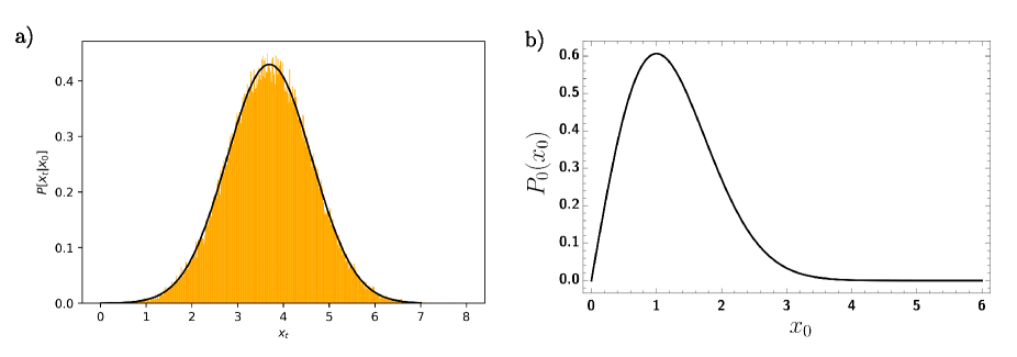
Figure 1: a) Conditional probability with $x_{0}=10,T,k=1,g=0.1$ and its numerical simulation of histogram in orange. b) Normalized canonical initial distribution with $g,T,k=1$.

The conditional probability is an important quantity in the derivation of the heat distribution. For the logarithm-harmonic case, it could be derived by path integrals giampaoli_exact_1999 or via the Fokker-Planck equation ryabov2015stochastic ; dechant_solution_2011 . The normalized conditional probability is given by :

$$P\left[x_{t},t|x_{0},0\right]=\frac{x_{0}\mathrm{e}^{(\nu+2)kt}}{2\frac{T}{k}e^{kt}\sinh{kt}}\left(\frac{x}{x_{0}}\right)^{\nu+1}\exp\left(-\frac{x_{t}^{2}\mathrm{e}^{2kt}+x_{0}^{2}}{4\frac{T}{k}e^{kt}\sinh{kt}}\right)\mathrm{I}_{\nu}\left(\frac{x_{t}x_{0}\mathrm{e}^{kt}}{2\frac{T}{k}e^{kt}\sinh{kt}}\right),$$ (4)

which is the same conditional probability derived in ryabov_brownian_2015 , but here we work with $k$ as a constant. This distribution is plotted in figure 2 a). We also the results from a simulation of this distribution, which is a sort of preview for the simulation of the heat distribution.

Since there is not any changes of parameters of the system, there is no work made on the system. Consequently, the stochastic thermodynamics of such a system is characterized solely by the heat. Following Sekimoto sekimoto2010stochastic , the heat is defined as the energy exchanged between the particle and the heat bath, which is

$$Q[x(t)]=\int_{0}^{t}\left(-\dot{x}+\eta(t)\right)dx$$ (5)

where the integral is defined in the Stratonovich prescription, which is an appropriate prescription to work with in stochastic thermodynamics bo_functionals_2019 . Using the Langevin equation 1 we derive the more simple formula

$$Q[x(t)]=\frac{k}{2}(x_{t}^{2}-x_{0}^{2})-g\log{\left(\frac{x_{t}}{x_{0}}\right)}$$ (6)

where one can notice that the heat is just the difference in the internal energy $\Delta U=Q[x]$, besides the fact that the heat can be written in terms of the final and initial points of the trajectory. We will see in the next section that the heat exhibits a non-trivial statistical behavior.

III Derivation of the Heat distribution

The heat, being a functional of the trajectory, has the conditional probability

$$P(Q|Q=Q[x])=\delta(Q-Q[x]).$$ (7)

It emphasizes that the random values of $Q$ are given by the trajectory-dependent formula $Q[x]$. In the studied case, the heat only depends on the initial and final points of the trajectory. Therefore, the probability distribution for the heat will be given by

$$P(Q)=\int dx_{t}dx_{0}P_{0}(x_{0})P[x_{t},t|x_{0},0]\delta(Q-Q[x]).$$ (8)

Moreover, we can rewrite 8 as

$$P(Q)=\int\frac{d\lambda}{2\pi}e^{i\lambda Q}Z(\lambda),$$ (9)

where

$$Z(\lambda)=\int dx_{t}\int dx_{0}P_{0}(x_{0})P[x_{t},t|x_{0},0]\exp(-i\lambda Q[x(t)]).$$ (10)

In the above formula, we just write the Dirac delta as an integral over $\lambda$. This formula is useful since allows us to identify $Z(\lambda)$ as the characteristic function.

The integrals in $Z(\lambda)$ can be carried analytically. But, the calculations are long, and the manipulations can be simplified using Mathematica Mathematica ; abramowitz1988handbook . The important thing to notice is the following integral identities:

$$\int_{0}^{\infty}I_{\nu}(ax)x^{b}e^{-cx^{2}}dx=2^{-\nu-1}a^{\nu}c^{\frac{1}{2}(-b-\nu-1)}\Gamma\left(\frac{1}{2}(b+\nu+1)\right)\,_{1}\tilde{F}_{1}\left(\frac{1}{2}(b+\nu+1);\nu+1;\frac{a^{2}}{4c}\right),$$ (11)

where ${}_{1}\tilde{F}_{1}$ is the regularized Kummer confluent hypergeometric function abramowitz1988handbook , and the conditions $a>0,b>-1,c>0$ have to be satisfied. And

$$\int_{0}^{\infty}{}_{1}\tilde{F}_{1}\left(a;b;cx^{2}\right)x^{d}e^{-fx^{2}}=\frac{1}{2}f^{-\frac{d}{2}-\frac{1}{2}}\Gamma\left(\frac{d+1}{2}\right)\,{}_{2}\tilde{F}_{1}\left(a,\frac{d+1}{2};b;\frac{c}{f}\right),$$ (12)

where ${}_{2}\tilde{F}_{1}$ is the regularized Gaussian hypergeometric function abramowitz1988handbook , and $d>-1$. The identities are used to integrate over $x_{t}$ and $x_{0}$. We use Eq. 11 to integrate over $x_{t}$ and Eq. 12 to integrate over $x_{0}$.

After integrating over $x_{t}$ and $x_{0}$ we find $Z(\lambda)$, which is written explicit in the next section (see Eq. 13). With $Z(\lambda)$ we still need to integrate over $\lambda$ to find the probability distribution. This integration can only be carried numerically, and the result is plotted in figure 2 a).

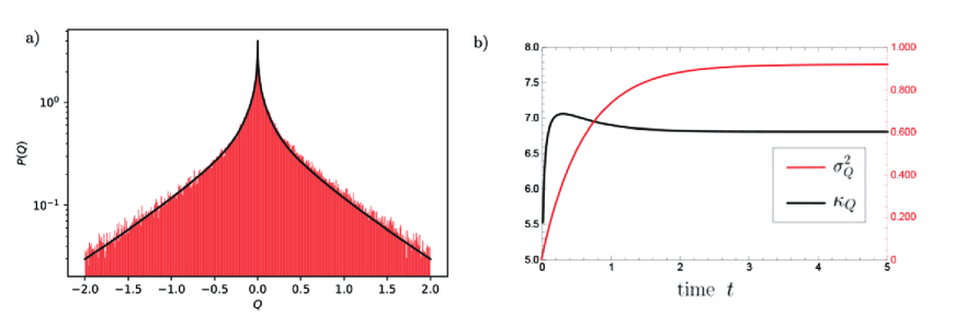
Figure 2: a) Heat distribution in logarithm scale with simulation values. b) Plot of the variance and the kurtosis. Variance (red line) with the vertical axis on the right (red axis) and kurtosis (black line) with the vertical axis on the left (black axis). We only have kurtosis and variance, since the mean and skewness are zero. The parameters values are $g=0.1,k=1,T=1,t=1$.

IV Characteristic Function and Moments

Even though the probability density needs to be calculated numerically, the characteristic function is achieved naturally as an intermediary step in the derivation of the probability density. The characteristic function is then

$$Z(\lambda)=\frac{(2k)^{\frac{g+T}{T}}}{\Gamma\left(\frac{g+T}{2T}\right)^{2}}\left(2\sinh{kt}\right)^{-\frac{g+T}{2T}}f(\lambda)^{-z_{\lambda}}f({-\lambda})^{-z_{\lambda}-ig\lambda}\Gamma\left(z_{\lambda}\right)\Gamma\left(z_{\lambda}+ig\lambda\right)\times$$

$${}_{2}F_{1}\left(z_{\lambda},z_{\lambda}+ig\lambda;\frac{g+T}{2T};\frac{k^{2}\text{csch}^{2}(kt)}{\coth(kt)(\coth(kt)+2)k^{2}+k^{2}+4T^{2}\lambda^{2}}\right),$$ (13)

where we defined the functions

$$f(\lambda)=(k-2iT\lambda+k\coth{kt}),$$ (14)

$$z_{\lambda}=\frac{g+T-igT\lambda}{2T},$$ (15)

for shortness sake, and the function ${}_{2}F_{1}(...)$ is the Gaussian hypergeometric function abramowitz1988handbook . With the above formula, we can simply check that the normalization of the probability is satisfied

$$Z(0)=1.$$ (16)

IV.1 Moments

With the characteristic function 13, we can calculate all the moments of the distribution, characterizing the fluctuations of the heat. The moments are given by

$$\langle Q^{n}\rangle=(-i)^{n}\frac{\partial^{n}Z(\lambda)}{\partial\lambda^{n}}\mid_{\lambda=0}.$$ (17)

Then, using the above formula, we can calculate the mean and the second moment:

$$\langle Q\rangle=-i\frac{\partial Z}{\partial\lambda}\mid_{\lambda=0}=0,$$ (18)

$$\langle Q^{2}\rangle=\frac{1}{4}\left(g^{2}\mathcal{J}(t)\sqrt{1-e^{-2kt}}e^{-\frac{gkt}{T}}\left(e^{2kt}-1\right)^{\frac{g}{2T}}+2g^{2}\psi^{(1)}\left(\frac{g+T}{2T}\right)+\frac{8Te^{-kt}(-2gk+g+T)\sinh(kt)}{k^{2}}\right),$$ (19)

where $\mathcal{J}(t)$ is written in terms of the Gaussian hypergeometric functions

$$\mathcal{J}(t)=\;_{2}F_{1}^{(0,2,0,0)}\left(\frac{g+T}{2T},\frac{g+T}{2T},\frac{g+T}{2T},e^{-2kt}\right)+$$ (20)

$$-2\;_{2}F_{1}^{(1,1,0,0)}\left(\frac{g+T}{2T},\frac{g+T}{2T},\frac{g+T}{2T},e^{-2kt}\right)+\;_{2}F_{1}^{(2,0,0,0)}\left(\frac{g+T}{2T},\frac{g+T}{2T},\frac{g+T}{2T},e^{-2kt}\right),$$

with ${}_{2}F_{1}^{(n,m,l,0)}=\partial^{3}_{n,m,l}\left({}_{2}F_{1}(n,m,l)\right)$, being the derivatives over the arguments of the Gaussian hypergeometric function. Because the mean is zero, the second moment is the variance, that is $\sigma_{Q}^{2}=\langle Q^{2}\rangle$. Apart from the complicated dependence in the parameters, the variance 19 has a stationary behavior, which can be seen in figure 2 and derived analytically. For $t\rightarrow\infty$ the variance becomes

$$\lim_{t\rightarrow\infty}\sigma^{2}_{Q}=\frac{1}{4}\left(2g^{2}\psi^{(1)}\left(\frac{g+T}{2T}\right)+\frac{4T(-2gk+g+T)}{k^{2}}\right),$$ (21)

where $\psi^{(1)}$ is the Poly-Gamma function abramowitz1988handbook .

Moving forward, one can show that the third moment $\langle Q^{3}\rangle$ is also zero. This means that the skewness is null and suggests that the distribution could be symmetric around the mean (a behavior that can be qualitatively observed in Figure 2 a), and numerically checked). As expected by checking the shape of the distribution in figure 2 a). With the mean, variance, and skewness, it is only missing the kurtosis. The excess kurtosis for our case will simplified by the formula

$$\kappa_{Q}=\frac{\langle Q^{4}\rangle}{\langle Q^{2}\rangle^{2}}-3.$$

This gives information about the shape of the distribution darlington_is_1970 . By figure 2 b) one can see that $\kappa_{Q}>-3$, which means that the distribution is leptokurtic darlington_is_1970 , meaning that the distribution in figure 2 a) has fatter tails than the normal distribution. Besides, this expression could have been written analytically, due to Eq. 17, but that we opt to omit here due to the extensive size of the expression. Nevertheless, the behavior is plotted in figure 2.

The graph in figure 2 b) suggests that the even momenta of the heat reach stationary values. This leads us to the calculation of the asymptotic of the characteristic function $Z(\lambda)$, which will be given by

$$\lim_{t\rightarrow\infty}Z(\lambda)=Z(\lambda,\infty)=\frac{(2k)^{\frac{g+T}{T}}}{\Gamma\left(\frac{g+T}{2T}\right)^{2}}\phi(\lambda)\;_{2}F_{1}\left(z_{\lambda},z_{\lambda}+ig\lambda;\frac{g+T}{2T};0\right),$$ (22)

where

$$\phi(\lambda)=\lim_{t\rightarrow\infty}f(\lambda)^{-z_{\lambda}}f({-\lambda})^{-z_{\lambda}-ig\lambda}\Gamma\left(z_{\lambda}\right)\Gamma\left(z_{\lambda}+ig\lambda\right),$$ (23)

is finite and was used for shortening the notation. Due to the non-trivial dependence on $\lambda$, even in the asymptotic limit, the characteristic function cannot be integrated analytically to yield the expression of the heat distribution.

V Numerical Simulations

We can compare our results with numerical simulations, which give an indirect validation of the results. To generate the initial distribution of the initial position, we use the “rejection method”, where we used a uniform random variable to select the random points that obey the probability in Eq. 3. Using a fourth-order Runge-Kutta tocino_rungekutta_2002 , we integrate the SDE in Eq. 1, evolving the system up to $t=1$. The system studied has a singularity in $x=0$, which is not physically allowed, since we have an asymmetric trap, as pointed out in section II. However, due to numerical errors, the simulation of the particle’s position can become negative. One way to avoid this is to increase the precision of the numerical simulation. With the ensemble of trajectories generated, we can measure the heat Eq. 6. Measuring different values of the heat, we can plot on a histogram and compare with the theoretical result.

The histogram and the theoretical result are plotted in figure 1, fitting the exact curve quite well, therefore indirectly validating our results via the numerical simulations.

VI Discussion and Conclusion

In the present paper, we have studied a diffusive system in a logarithm-harmonic potential. This system presents a simple stochastic energetic characterization: it is described only by heat and internal energy. Herein, we derived the heat distribution exactly. The result is compared with numerical simulations and it is in good accordance. Moreover, we derive analytically the characteristic function for the heat probability distribution, allowing us to calculate all the moments of the distribution, and to characterize all the statistical behavior of the system.

The heat distribution is symmetric in $Q$, which means that $P(Q)=P(-Q)$ in agreement with the vanishing skewness and figure 2 a). We must notice that this is a consequence of choosing an equilibrated initial distribution. This equilibrium, non entropy producing dynamics, implies that the particle has the same chance of absorbing or losing energy from the heat bath. This symmetric behavior can be understood by noticing that the particle can equilibrate with the heat bath, a behavior which is not present in the case without the harmonic contribution paraguassu_heat_2021 . Moreover, if we compare with the single harmonic case chatterjee_exact_2010 , one can see that our distribution has a similar shape to the heat distribution in chatterjee_exact_2010 , but in the presence of the logarithm potential the divergence in $Q=0$ is not present. Moreover, besides the apparent fast decay of the distribution, one can show that the tails of the distribution decay slower than an exponential decay, forbidding the usual analysis via large deviation theory touchette_large_2009 .

The fluctuations of the heat are described by the characteristic function $Z(\lambda)$. In our case, $Z(\lambda)$ has a non-trivial dependence due to the Gaussian hypergeometric function, together with the Gamma functions. That not withstanding, by means of $Z(\lambda)$, we calculate the mean, variance, skewness, and kurtosis. The mean, skewness, and any odd moment are zero, as expected since the probability is symmetric in $Q$. Moreover, as plotted in figure 2 b), the evolution of the variance and the kurtosis reach a stationary value, which can be understood as a consequence of the particle starting comming to equilibrium with the heat bath. We calculate the stationary behavior for the variance and also for the characteristic function. Writing in terms of Poly-Gamma functions, Gamma functions, and Gaussian hypergeometric, the asymptotic characteristic function is still not integrable in $\lambda$. Reinforcing the non-trivial nature of the statistical behavior of the heat.

In conclusion, we have obtained exact results for the heat distribution, the characteristic function, and its moments. Our results are compared with numerical simulations, showing its consistency. The results are discussed and compared with the literature, giving new insights into the problem. Moreover, our finding extends the list of characterized heat distribution in stochastic thermodynamics.

References

References

- (1) Oliveira M J d 2020 Revista Brasileira de Ensino de Física 42
- (2) Ciliberto S 2017 Phys. Rev. X 7 021051 publisher: American Physical Society URL https://link.aps.org/doi/10.1103/PhysRevX.7.021051
- (3) Seifert U 2012 Reports on progress in physics 75 126001
- (4) Sekimoto K 2010 Stochastic energetics vol 799 (Springer)
- (5) Paraguassú P V and Morgado W A M 2021 J. Stat. Mech. 2021 023205 ISSN 1742-5468 publisher: IOP Publishing URL https://doi.org/10.1088/1742-5468/abda25
- (6) Chatterjee D and Cherayil B J 2010 Phys. Rev. E 82 051104 ISSN 1539-3755, 1550-2376 URL https://link.aps.org/doi/10.1103/PhysRevE.82.051104
- (7) Chatterjee D and Cherayil B J 2011 J. Stat. Mech. 2011 P03010 ISSN 1742-5468 URL https://iopscience.iop.org/article/10.1088/1742-5468/2011/03/P03010
- (8) Ghosal A and Cherayil B J 2016 J. Stat. Mech. 2016 043201 ISSN 1742-5468 publisher: IOP Publishing URL https://doi.org/10.1088/1742-5468/2016/04/043201
- (9) Saha B and Mukherji S 2014 J. Stat. Mech. 2014 P08014 ISSN 1742-5468 URL https://iopscience.iop.org/article/10.1088/1742-5468/2014/08/P08014
- (10) Kuśmierz \, Rubi J M and Gudowska-Nowak E 2014 J. Stat. Mech. 2014 P09002 ISSN 1742-5468 publisher: IOP Publishing URL https://doi.org/10.1088/1742-5468/2014/09/p09002
- (11) Chvosta P, Lips D, Holubec V, Ryabov A and Maass P 2020 J. Phys. A: Math. Theor. 53 275001 ISSN 1751-8113, 1751-8121 URL https://iopscience.iop.org/article/10.1088/1751-8121/ab95c2
- (12) Goswami K 2019 Phys. Rev. E 99 012112 publisher: American Physical Society URL https://link.aps.org/doi/10.1103/PhysRevE.99.012112
- (13) Goswami K 2019 Physica A: Statistical Mechanics and its Applications 525 223–233 ISSN 03784371 URL https://linkinghub.elsevier.com/retrieve/pii/S0378437119302857
- (14) Goswami K 2021 Physica A: Statistical Mechanics and its Applications 566 125609 ISSN 0378-4371 URL https://www.sciencedirect.com/science/article/pii/S0378437120309079
- (15) Kwon C, Noh J D and Park H 2013 Phys. Rev. E 88 062102 publisher: American Physical Society URL https://link.aps.org/doi/10.1103/PhysRevE.88.062102
- (16) Jiménez-Aquino J and Sánchez-Salas N 2018 Physica A: Statistical Mechanics and its Applications 509 12–19 ISSN 03784371 URL https://linkinghub.elsevier.com/retrieve/pii/S0378437118306782
- (17) Joubaud S, Garnier N B and Ciliberto S 2007 J. Stat. Mech. 2007 P09018–P09018 ISSN 1742-5468 publisher: IOP Publishing URL https://doi.org/10.1088/1742-5468/2007/09/p09018
- (18) Gomez-Solano J R, Petrosyan A and Ciliberto S 2011 Phys. Rev. Lett. 106 200602 publisher: American Physical Society URL https://link.aps.org/doi/10.1103/PhysRevLett.106.200602
- (19) Imparato A, Peliti L, Pesce G, Rusciano G and Sasso A 2007 Phys. Rev. E 76 050101 publisher: American Physical Society URL https://link.aps.org/doi/10.1103/PhysRevE.76.050101
- (20) Imparato A, Jop P, Petrosyan A and Ciliberto S 2008 J. Stat. Mech. 2008 P10017 ISSN 1742-5468 URL https://iopscience.iop.org/article/10.1088/1742-5468/2008/10/P10017
- (21) Ryabov A, Dierl M, Chvosta P, Einax M and Maass P 2013 J. Phys. A: Math. Theor. 46 075002 ISSN 1751-8121 publisher: IOP Publishing URL https://doi.org/10.1088/1751-8113/46/7/075002
- (22) Holubec V, Dierl M, Einax M, Maass P, Chvosta P and Ryabov A 2015 Phys. Scr. T165 014024 ISSN 0031-8949, 1402-4896 URL https://iopscience.iop.org/article/10.1088/0031-8949/2015/T165/014024
- (23) Ryabov A 2015 Stochastic dynamics and energetics of biomolecular systems (Springer)
- (24) Leibovich N, Dechant A, Lutz E and Barkai E 2016 Phys. Rev. E 94 052130 publisher: American Physical Society URL https://link.aps.org/doi/10.1103/PhysRevE.94.052130
- (25) Hirschberg O, Mukamel D and Schütz G M 2011 Phys. Rev. E 84 041111 publisher: American Physical Society URL https://link.aps.org/doi/10.1103/PhysRevE.84.041111
- (26) Aghion E, Kessler D A and Barkai E 2019 Phys. Rev. Lett. 122 010601 ISSN 0031-9007, 1079-7114 URL https://link.aps.org/doi/10.1103/PhysRevLett.122.010601
- (27) Dechant A, Lutz E, Kessler D A and Barkai E 2012 Phys. Rev. E 85 051124 publisher: American Physical Society URL https://link.aps.org/doi/10.1103/PhysRevE.85.051124
- (28) Barkai E, Aghion E and Kessler D A 2014 Phys. Rev. X 4 021036 ISSN 2160-3308 URL https://link.aps.org/doi/10.1103/PhysRevX.4.021036
- (29) Kessler D A and Barkai E 2010 Phys. Rev. Lett. 105 120602 ISSN 0031-9007, 1079-7114 URL https://link.aps.org/doi/10.1103/PhysRevLett.105.120602
- (30) Ray S and Reuveni S 2020 J. Chem. Phys. 152 234110 ISSN 0021-9606 publisher: American Institute of Physics URL https://aip.scitation.org/doi/abs/10.1063/5.0010549
- (31) Bray A J 2000 Phys. Rev. E 62 103–112 publisher: American Physical Society URL https://link.aps.org/doi/10.1103/PhysRevE.62.103
- (32) Ryabov A, Berestneva E and Holubec V 2015 The Journal of Chemical Physics 143 114117 ISSN 0021-9606, 1089-7690 URL http://aip.scitation.org/doi/10.1063/1.4931474
- (33) Fogedby H C and Metzler R 2007 Phys. Rev. Lett. 98 070601 publisher: American Physical Society URL https://link.aps.org/doi/10.1103/PhysRevLett.98.070601
- (34) Lo C C, Amaral L A N, Havlin S, Ivanov P C, Penzel T, Peter J H and Stanley H E 2002 EPL 57 625 ISSN 0295-5075 publisher: IOP Publishing URL https://iopscience.iop.org/article/10.1209/epl/i2002-00508-7/meta
- (35) Campisi M, Zhan F, Talkner P and Hänggi P 2012 Phys. Rev. Lett. 108 250601 publisher: American Physical Society URL https://link.aps.org/doi/10.1103/PhysRevLett.108.250601
- (36) Manning G S 1969 J. Chem. Phys. 51 934–938 ISSN 0021-9606 publisher: American Institute of Physics URL https://aip.scitation.org/doi/10.1063/1.1672158
- (37) Liboff R L 1966 Phys. Rev. 141 222–227 publisher: American Physical Society URL https://link.aps.org/doi/10.1103/PhysRev.141.222
- (38) Paraguassú P V, Aquino R and Morgado W A M 2021 arXiv:2102.09115 [cond-mat] ArXiv: 2102.09115 URL http://arxiv.org/abs/2102.09115
- (39) Gupta D and Sivak D A 2021 arXiv:2103.09358 [cond-mat] ArXiv: 2103.09358 URL http://arxiv.org/abs/2103.09358
- (40) Fogedby H C 2020 J. Stat. Mech. 2020 083208 ISSN 1742-5468 publisher: IOP Publishing URL https://doi.org/10.1088/1742-5468/aba7b2
- (41) Crisanti A, Sarracino A and Zannetti M 2017 Phys. Rev. E 95 052138 publisher: American Physical Society URL https://link.aps.org/doi/10.1103/PhysRevE.95.052138
- (42) Rosinberg M L, Tarjus G and Munakata T 2016 EPL 113 10007 ISSN 0295-5075 publisher: IOP Publishing URL https://doi.org/10.1209/0295-5075/113/10007
- (43) Kim K, Kwon C and Park H 2014 Phys. Rev. E 90 032117 ISSN 1539-3755, 1550-2376 URL https://link.aps.org/doi/10.1103/PhysRevE.90.032117
- (44) Fogedby H C and Imparato A 2009 J. Phys. A: Math. Theor. 42 475004 ISSN 1751-8121 publisher: IOP Publishing URL https://doi.org/10.1088/1751-8113/42/47/475004
- (45) Giampaoli J A, Strier D E, Batista C, Drazer G and Wio H S 1999 Phys. Rev. E 60 2540–2546 publisher: American Physical Society URL https://link.aps.org/doi/10.1103/PhysRevE.60.2540
- (46) Dechant A, Lutz E, Barkai E and Kessler D A 2011 J Stat Phys 145 1524–1545 ISSN 0022-4715, 1572-9613 URL http://link.springer.com/10.1007/s10955-011-0363-z
- (47) Bo S, Lim S H and Eichhorn R 2019 J. Stat. Mech. 2019 084005 ISSN 1742-5468 publisher: IOP Publishing URL https://doi.org/10.1088/1742-5468/ab3111
- (48) Inc W R Mathematica, Version 12.2 champaign, IL, 2020 URL https://www.wolfram.com/mathematica
- (49) Abramowitz M, Stegun I A and Romer R H 1988 Handbook of mathematical functions with formulas, graphs, and mathematical tables
- (50) Darlington R B 1970 The American Statistician 24 19–22 ISSN 0003-1305 publisher: Taylor & Francis _eprint: https://doi.org/10.1080/00031305.1970.10478885 URL https://doi.org/10.1080/00031305.1970.10478885
- (51) Tocino A and Ardanuy R 2002 Journal of Computational and Applied Mathematics 138 219–241 ISSN 0377-0427 URL https://www.sciencedirect.com/science/article/pii/S0377042701003806
- (52) Touchette H 2009 Physics Reports 478 1–69 ISSN 03701573 URL https://linkinghub.elsevier.com/retrieve/pii/S0370157309001410