Dissipative superfluid hydrodynamics for the unitary Fermi gas

Abstract

In this work we establish constraints on the temperature dependence of the shear viscosity $\eta$ in the superfluid phase of a dilute Fermi gas in the unitary limit. Our results are based on analyzing experiments that measure the aspect ratio of a deformed cloud after release from an optical trap. We discuss how to apply the two-fluid formalism to the unitary gas, and provide a suitable parametrization of the equation of state. We show that in expansion experiments the difference between the normal and superfluid velocities remains small, and can be treated as a perturbation. We find that expansion experiments favor a shear viscosity that decreases significantly in the superfluid regime. Using an exponential parametrization we find $\eta(T_{c}/(2T_{F}))\mathrel{\hbox to0.0pt{\lower 4.0pt\hbox{$\sim$}\hss}\raise 1.0pt\hbox{$<$}}0.37\,\eta(T_{c}/T_{F})$, where $T_{c}$ is the critical temperature, and $T_{F}$ is the local Fermi temperature of the gas.

I Introduction

The dilute Fermi gas at unitarity has emerged as an important example of a strongly correlated quantum fluid Bloch:2007 ; Giorgini:2008 . Measurements of equilibrium and non-equilibrium properties provide important benchmarks for a variety of physical systems, ranging from dilute neutron matter in neutron stars to the quark gluon plasma probed in relativistic heavy ion collisions. The unitary Fermi gas is a system of non-relativistic spin-1/2 particles interacting via an interaction of zero range tuned to infinite scattering length. This means that the system is strongly interacting, but the only scales in the problem are those that can be defined in the non-interacting gas, for example the Fermi momentum $k_{F}=(3\pi^{2}n)^{1/3}$, where $n$ is the density of the gas. From the Fermi momentum we can construct the Fermi energy $E_{F}=k_{F}^{2}/(2m)$, and the Fermi temperature $k_{B}T_{F}=E_{F}$, where $k_{B}$ is the Boltzmann constant. As an example, consider the superfluid transition in a unitary Fermi gas. Based on dimensional analysis, the critical temperature must be proportional to the local Fermi temperature, $T_{c}\sim T_{F}$. Indeed, experiments find $T_{c}=0.167(3)T_{F}$ Ku:2011 .

A remarkable property of the unitary Fermi gas is nearly perfect hydrodynamic flow Schafer:2009dj ; Adams:2012th ; Schaefer:2014awa ; Schafer:2007pr ; Turlapov:2007 , originally discovered in OHara:2002 . In this experiment, the authors observed nearly ideal flow in a dilute unitary Fermi gas after release from a deformed trap. The deformation of the trap implies that pressure gradients in the short (transverse) direction of the trap lead to preferential acceleration in this direction. As a consequence, the aspect ratio of the cloud changes from being elongated in the longitudinal direction to being elongated in the transverse direction. Viscosity counteracts this behavior, and detailed studies of the time evolution can be used to extract the shear viscosity as a function of $T/T_{F}$.

Shear viscosity is a dimensionful quantity, and it is natural to consider the dimensionless ratios $\eta/n$ or $\eta/s$, where $s$ is the entropy density. We have also set $\hbar=k_{B}=1$, where $\hbar$ is Planck’s constant, and $k_{B}$ is Boltzmann’s constant. Previous analysis finds that for $T>T_{F}$ the shear viscosity of the gas can be understood in terms of kinetic theory, and that in this regime $\eta/n>1$ Bluhm:2015bzi . Near the critical temperature the shear viscosity enters the quantum regime, $\eta/n<1$, and the viscosity is only weakly temperature dependent. At $T_{c}$, we find $\eta/n\simeq 0.4$ Bluhm:2017rnf , in agreement with calculations based on the Kubo relation and resummed perturbation theory Enss:2010qh , see also Hofmann:2011qs ; Hofmann:2019jcj ; Frank:2020oef .

Our main goal in the present work is to constrain the behavior of $\eta/n$ below the superfluid phase transition using existing expansion experiments, in particular the results of Joseph et al. Joseph:2014 . Several, qualitatively different, predictions and results regarding the behavior of $\eta/n$ below $T_{c}$ can be found in the literature. In Ref. Rupak:2007vp we argued that for $T\ll T_{c}$ kinetic theory in terms of phonon quasi-particles is reliable, and that it predicts that $\eta/n$ grows rapidly as $T/T_{F}\to 0$. On the other hand, Ref. Guo:2010 proposed a different quasi-particle model, which predicts $\eta/n\to 0$ as $T\to 0$. This behavior is seen in the Quantum Monte Carlo calculation of Wlazlowski:2013owa , and in the simplified experimental analysis in Joseph:2014 . A recent experimental study of sound attenuation in a unitary Fermi gas finds that sound diffusivity is approximately constant below $T_{c}$ Patel:2019 . Different behaviors are also seen in the two isotopes of helium. In ⁴He the viscosity is dominated by rotons and phonons. It is approximately constant near $T_{c}$, and grows very steeply as $T\to 0$ Schafer:2009dj . In ³He, on the other hand, the viscosity shows a steep drop below $T_{c}$ Guo:2010 ; Vollhardt:1990 .

The basic tool for analyzing the expansion experiment below $T_{c}$ is superfluid (two-fluid) hydrodynamics. When solving the two-fluid equations in an expanding system, careful attention has to be paid to the frame dependence of the equations of motion. We review this issue in Section II and III. Section  IV discusses simplifications that appear if the fluid is scale invariant, as is the case for the unitary Fermi gas. Sections II-IV can be skipped if the reader is primarily interested in the analysis of the experiments of Joseph et al. Joseph:2014 . Simple solution of the two-fluid equations are discussed in Sect. V. We discuss an approach based on treating the difference between the superfluid and normal velocities as a small parameter, and present an analysis of the experimental data using this method in Sect. VI. We conclude in Sect. VII, and details regarding the equation of state and the initial conditions for two-fluid hydrodynamics are discussed in several appendices.

II Superfluid hydrodynamics

Fluid dynamics is based on conservation laws, combined with approximate local thermodynamic equilibrium. Thermodynamic relations are encoded in an equation of state, which can be measured in a fluid at rest in the laboratory frame. In this section we review how this information is used in the fluid dynamic description of an expanding fluid. For simplicity, consider first a normal fluid, for example the unitary Fermi gas above $T_{c}$. There are five hydrodynamic variables, the mass density $\rho$, the energy density ${\cal E}$ (or, alternatively, the entropy density $s$), and the mass current $\vec{\jmath}$. Note that the mass current is equal to the density of momentum, so that the total momentum of the fluid is the integral of $\vec{\jmath}$ over the volume occupied by the fluid.

For a fluid element centered at position $\vec{x}$ with mass current $\vec{\jmath}\,(\vec{x})$ there is a Galilean boost with boost velocity $\vec{v}=\vec{\jmath}/\rho$ that transforms the conserved charges into the local rest frame of the fluid, defined by $\vec{\jmath}\,(\vec{x})=0$. In this frame the energy density of the fluid is ${\cal E}_{0}={\cal E}-\vec{\jmath}^{\;2}/(2\rho)$, see App. A. The energy density in the rest frame satisfies the standard thermodynamic identity

$$d{\cal E}_{0}=\mu_{0}dn+Tds,$$ (1)

where $\mu_{0}$ is the chemical potential in the fluid rest frame and $n=\rho/m$ is the particle number density. The energy in the laboratory frame satisfies

$$d{\cal E}=\left(\mu_{0}-\frac{1}{2}m\vec{v}^{\,2}\right)dn+Tds+\vec{v}\cdot d\vec{\jmath}\,.$$ (2)

The pressure is given by the Legendre transform of equ. (2) with respect to $n,s$ and $\vec{\jmath}$. We obtain $P=\mu_{0}n+sT-{\cal E}_{0}$, and the pressure satisfies the Gibbs-Duhem relation $dP=nd\mu_{0}+sdT$.

In a superfluid there are three additional hydrodynamic variables, the components of the superfluid velocity $\vec{v}_{s}$. As a result, there no longer is a unique local frame in which the fluid is at rest. In this section we will follow Landau Landau-Hydro and consider thermodynamics in the restframe of the superfluid. The final result is of course independent of the choice of frame, and we describe thermodynamic relations in the rest frame of the normal fluid in App. B. The mass current in the frame of the superfluid is $\vec{\jmath}_{0}=\vec{\jmath}-\rho\vec{v}_{s}$. Using Galilean invariance we can determine the energy density in the superfluid rest frame

$${\cal E}_{s}={\cal E}-\vec{\jmath}_{0}\cdot\vec{v}_{s}-\frac{1}{2}\rho v_{s}^{2}\,,$$ (3)

We now view the energy density in the superfluid frame as a function of $\vec{\jmath}_{0}$,

$$d{\cal E}_{s}=\mu_{s}dn+Tds+\vec{w}\cdot d\vec{\jmath}_{0}\,,$$ (4)

where we have defined $\mu_{s}$, the chemical potential in the superfluid frame, and the velocity $\vec{w}$. For the energy in the lab frame equ. (4) implies

$$d{\cal E}=\mu_{\jmath_{0}}dn+Tds+\vec{v}_{n}\cdot d\vec{\jmath}_{0}\,+\vec{\jmath}\cdot d\vec{v}_{s}\,,$$ (5)

where

$$\mu_{\jmath_{0}}=\mu_{s}+\frac{1}{2}mv_{s}^{2}\,,$$ (6)

and we have defined $\vec{v}_{n}=\vec{w}+\vec{v}_{s}$, the velocity of the normal fluid. We note that $\vec{w}=\vec{v}_{n}-\vec{v}_{s}$ is Galilei invariant. We can perform a Legendre transformation with respect to $n,s$ and $\jmath_{0}$. We obtain the pressure

$$P=-{\cal E}_{s}+\mu_{s}n+Ts+\vec{\jmath}_{0}\cdot\vec{w}\,,$$ (7)

and the Gibbs-Duhem relation

$$dP=nd\mu_{s}+sdT+\vec{\jmath}_{0}\cdot d\vec{w}\,.$$ (8)

Based on Galilean invariance we can write $\vec{\jmath}_{0}=\rho_{n}\vec{w}$, which defines the normal fluid density $\rho_{n}$, as well as the superfluid density $\rho_{s}=\rho-\rho_{n}$. This definition leads to the standard two-fluid relation $\vec{\jmath}=\rho_{n}\vec{v}_{n}+\rho_{s}\vec{v}_{s}$. We note that

$$\rho_{n}=2\left.\frac{\partial P}{\partial w^{2}}\right|_{\mu_{s},T},$$ (9)

and $\rho_{n}\geq 0$ implies that at fixed $\mu_{s}$ the pressure increases with $|\vec{w}|$. Finally, we note that

$$P+{\cal E}=\mu_{s}n+Ts+\rho_{n}\vec{w}\cdot\vec{v}_{n}+\frac{1}{2}\rho v_{s}^{2}\,,$$ (10)

which will be useful in the following section.

III Conservation Laws

As in ordinary fluid dynamics there are conservation laws for the mass density, the momentum density, and the energy density of the fluid. Mass conservation is

$$\partial_{t}\rho+\vec{\nabla}\cdot\vec{\jmath}=0\,,$$ (11)

where $\rho=\rho_{n}+\rho_{s}$. The particle density is decomposed analogously, $n=n_{n}+n_{s}$. The mass equation does not receive any dissipative corrections. Momentum conservation is

$$\partial_{t}\jmath_{i}+\nabla_{j}\Pi_{ij}=0\,$$ (12)

where the stress tensor $\Pi_{ij}$ can be split into an ideal and a dissipative part, $\Pi_{ij}=\Pi^{(0)}_{ij}+\delta\Pi_{ij}$. The ideal part is

$$\Pi_{ij}^{(0)}=P\delta_{ij}+\rho_{n}(v_{n})_{i}(v_{n})_{j}+\rho_{s}(v_{s})_{i}(v_{s})_{j}\,.$$ (13)

Note that the stress tensor in the superfluid rest frame is $\Pi_{ij}^{(0,s)}=P\delta_{ij}+\rho_{n}w_{i}w_{j}$. This expression follows from Galilean invariance and the second law of thermodynamics. The transformation of $\Pi_{ij}$ under Galilean boosts is given in equ. (49). The dissipative terms are given by

$$\delta\Pi_{ij}=-\eta\sigma_{ij}-\zeta_{2}\delta_{ij}\left(\vec{\nabla}\cdot\vec{v}_{n}\right)-\zeta_{1}\vec{\nabla}\cdot\left(\rho_{s}\vec{w}\right)\,,$$ (14)

where $\eta$ is the shear viscosity, the shear tensor is defined by

$$\sigma_{ij}=\nabla_{i}(v_{n})_{j}+\nabla_{j}(v_{n})_{i}-\frac{2}{3}\delta_{ij}(\vec{\nabla}\cdot\vec{v}_{n})\,,$$ (15)

and $\zeta_{1,2}$ are bulk viscosities. In a scale invariant fluid both $\zeta_{1}$ and $\zeta_{2}$ vanish. Energy conservation is

$$\partial_{t}{\cal E}+\vec{\nabla}\cdot\vec{Q}=0$$ (16)

with $\vec{Q}=\vec{Q}^{(0)}+\delta\vec{Q}$. The ideal energy current in the superfluid rest frame is proportional to $\vec{w}$. Using the second law of thermodynamics one can show that $\vec{Q}^{(0,s)}=({\cal E}_{s}+P-n_{s}\mu_{s})\vec{w}$, and the energy current in the lab frame is

$$\vec{Q}^{(0)}=\left(\frac{\mu_{s}}{m}+\frac{v_{s}^{2}}{2}\right)\vec{\jmath}+sT\vec{v}_{n}+\rho_{n}\left(v_{n}^{2}-\vec{v}_{n}\cdot\vec{v}_{s}\right)\vec{v}_{n}\,.$$ (17)

We observe that with the help of equ. (10) the energy current $\vec{Q}^{(0)}$ can be expressed as

$$\vec{Q}^{(0)}=\vec{v}_{n}\left({\cal E}+P\right)-\rho_{s}\vec{w}\left(\frac{\mu_{s}}{m}+\frac{v_{s}^{2}}{2}\right)\,.$$ (18)

The dissipative correction is

$$\delta Q_{i}=-\kappa\nabla_{i}T+\delta\Pi_{ij}(v_{n})_{j}-\delta\chi\rho_{s}w_{i}\,,$$ (19)

where $\kappa$ is the thermal conductivity, and $\delta\chi$ is given in equ. (22). Finally, superfluid hydrodynamics requires an equation of motion for the superfluid velocity. We have

$$\partial_{t}\vec{v}_{s}+\vec{\nabla}\chi=0$$ (20)

with $\chi=\chi^{(0)}+\delta\chi$ and

$$\chi^{(0)}=\frac{\mu_{s}}{m}+\frac{v_{s}^{2}}{2}\,.$$ (21)

The dissipative term is

$$\delta\chi=\zeta_{4}\vec{\nabla}\cdot\vec{v}_{n}+\zeta_{3}\vec{\nabla}\left(\rho_{s}\vec{w}\right)\,.$$ (22)

In a scale invariant gas $\zeta_{4}$ vanishes Son:2005tj , but $\zeta_{3}$ is expected to be non-zero.

IV Unitary Fermi Gas

In a normal fluid the pressure is a function of two variables, $P=P(\mu_{0},T)$. In a scale invariant fluid we can write

$$P(\mu_{0},T)=m^{3/2}\mu_{0}^{5/2}p(T/\mu_{0}).$$ (23)

In general, the function $p(T/\mu)$ has to be determined from experiment. A parametrization of $p(T/\mu)$ for the dilute Fermi gas at unitarity can be found in Bluhm:2017rnf , and in App. C. In a superfluid the pressure is a function of three variables, $P(\mu_{s},T,\vec{w})$. Using scale invariance we can define a function $p_{s}$ of two variables,

$$P(\mu_{s},T,\vec{w})=m^{3/2}\mu_{s}^{5/2}p_{s}\left(\frac{T}{\mu_{s}},\frac{mw^{2}}{\mu_{s}}\right)\,,$$ (24)

and for small $w$ we can expand

$$P(\mu_{s},T,\vec{w})=P_{0}(\mu_{s},T)+P_{1}(\mu_{s},T)w^{2}=m^{3/2}\mu_{s}^{5/2}p_{s0}\left(\frac{T}{\mu_{s}}\right)+m^{5/2}\mu_{s}^{3/2}w^{2}p_{s1}\left(\frac{T}{\mu_{s}}\right)\,.$$ (25)

In a similar fashion, we can expand the density, $n=n_{0}+n_{1}w^{2}$, and the entropy density, $s=s_{0}+s_{1}w^{2}$. Note that for $\vec{w}=0$ we have $\mu_{s}=\mu_{0}$ so that the function $p_{s0}$ is determined by the pressure of a fluid at rest, $p_{s0}(T/\mu)=p(T/\mu)$. The function $p_{s1}$ is related to the normal fluid density

$$\rho_{n}=2m^{5/2}\mu_{s}^{3/2}p_{s1}\left(\frac{T}{\mu_{s}}\right)\,.$$ (26)

In fluid dynamics we have to determine the pressure using the values of the conserved charges. Consider first a normal scale invariant fluid. Given the energy density we can determine the energy density in the rest frame, ${\cal E}_{0}={\cal E}-\jmath^{2}/(2\rho)$. Using the Gibbs-Duhem relation we get

$${\cal E}_{0}=\left\{\mu_{0}\frac{\partial}{\partial\mu_{0}}+T\frac{\partial}{\partial T}-1\right\}P(\mu_{0},T)\,.$$ (27)

Using the universal form of the equation of state in equ. (23) this implies $P=\frac{2}{3}{\cal E}_{0}$ and

$$P=\frac{2}{3}\left\{{\cal E}-\frac{\jmath^{2}}{2\rho}\right\}\,.$$ (28)

We observe that the pressure can be determined without using the explicit form of the function $p(T/\mu)$. Note that if the fluid is not scale invariant, then we have to tabulate the equation of state in the form $P=P({\cal E}_{0},\rho)$ in order to determine the pressure. We also note that transport coefficients are functions of $T/\mu_{0}$. The determination of $T/\mu_{0}$ requires explicit knowledge of the function $p(T/\mu)$. A procedure for extracting $T/\mu_{0}$ was proposed in Bluhm:2017rnf . Consider the dimensionless ratio

$$x=\frac{2}{(2\pi)^{3/2}}\frac{(mP)^{3/2}}{n^{5/2}}\,.$$ (29)

The quantity $x$ is Galilean invariant, and purely a function of the inverse fugacity $\zeta=\exp(-\mu_{0}/T)$. The function $\zeta(x)$ can be determined from the function $p(T/\mu)$ defined above. Once $\zeta$ is determined we can compute the temperature from

$$T=G(x)\frac{P}{n}$$ (30)

where the dimensionless function $G(x)$ is also determined by $p(T/\mu)$, see App. C. Once $\zeta$ and $T$ are given, then the chemical potential is determined by $\mu=-T\log(\zeta)$.

We can now study the analogous problem in the superfluid phase. We first note that given the local energy density ${\cal E}$ we can compute ${\cal E}_{s}$ using equ. (3). This calculation only requires the hydrodynamic variables $\rho,\vec{\jmath}$ and $\vec{v}_{s}$. Furthermore, equ. (7) and (8) imply that

$${\cal E}_{s}=\left\{\mu_{s}\frac{\partial}{\partial\mu_{s}}+T\frac{\partial}{\partial T}+\vec{w}\frac{\partial}{\partial\vec{w}}-1\right\}P(\mu_{s},T,w)\,.$$ (31)

Using the equation of state of the unitary gas at $O(w^{2})$ we get

$$P=\frac{2}{3}\left\{{\cal E}_{s}-\frac{1}{2}\vec{\jmath}_{0}\cdot\vec{w}\right\}\,.$$ (32)

This result is more difficult to use than equ. (28) because, whereas ${\cal E}$, ${\cal E}_{s}$, and $\jmath_{0}$ are (primary) hydrodynamic variables, $\vec{w}$ is determined by the equation of state, $\vec{w}=\vec{\jmath}_{0}/\rho_{n}$ with $\rho_{n}=\rho_{n}(\rho,{\cal E}_{s},\jmath_{0})$. One possible approach is to tabulate the function $\rho_{n}(\rho,{\cal E}_{s},\jmath_{0})$ for the equation of state given in equ. (24). Another option is to solve for $\rho_{n}$ and $P$ perturbatively in $w^{2}/\mu_{s}$. In the perturbative approach we set

$$P(\{w^{0}\})=\frac{2}{3}{\cal E}_{s}$$ (33)

and define

$$x(\{w^{0}\})=\frac{2}{(2\pi)^{3/2}}\frac{(mP(\{w^{0}\})^{3/2}}{n^{5/2}}\,.$$ (34)

Here, $P(\{w^{0}\})$ denotes the pressure at order $w^{0}$, that is the exact pressure up to corrections of order $O(w^{2})$. We can compute the inverse fugacity at this order in the expansion, $\zeta\simeq\zeta(x(\{w^{0}\}))$, and the result determines the normal fluid fraction at $O(w^{0})$

$$\left(\frac{\rho_{n}}{\rho}\right)_{\{w^{0}\}}=\left.\frac{2p_{s1}(x)}{\frac{5}{2}p_{s0}(x)-xp_{s0}^{\prime}(x)}\right|_{x=x(\{w^{0}\})}\,.$$ (35)

This result can now be used to compute the pressure at $O(w^{2})$,

$$P(\{w^{2}\})=\frac{2}{3}\left\{{\cal E}_{s}-\left(\frac{\jmath^{2}_{0}}{2\rho}\right)\left(\frac{\rho}{\rho_{n}}\right)_{\{w^{0}\}}\right\}\,.$$ (36)

If needed, these results can be used to compute $\mu_{s}$ and $T$ at order $w^{2}$.

V Simple solutions of the two-fluid equations

It is interesting to note that there are some simple solutions to the equations of superfluid hydrodynamics that are relevant to trapped atomic gases. We first observe that the solution of the hydrostatic equation carries over directly from the normal fluid case. Consider a fluid confined by an external potential $V_{\it ext}(x)$. A static solution of the fluid dynamic equations is given by

$$n(\vec{x})=n(\mu_{s}(\vec{x}),T)\,\hskip 28.45274pt\mu_{s}(\vec{x})=\mu_{c}-V_{\it ext}(\vec{x})$$ (37)

with $\vec{v}_{n}=\vec{v}_{s}=0$. This follows directly from the Gibbs-Duhem relation $\vec{\nabla}P=n\vec{\nabla}\mu_{s}$ for $T={\it const}$ and $\vec{w}=0$. We are mostly interested in approximately harmonic potentials of the form $V_{\it ext}(\vec{x})=m\omega_{i}^{2}x_{i}^{2}/2$. A number of authors have considered small oscillations around the hydrostatic case, see, for example Zaremba:1999 ; Stringari:2013 . The solutions are analogous to first and second sound modes in an infinite system.

In the normal fluid case there is a simple exact scaling solution to the Euler equation that describes the expansion after a confining harmonic potential is turned off. For this solution the density expands by a scale transformation, $n(x_{i},t)=n(x_{i}/b_{i}(t),t\!=\!0)$, where $n(x_{i},0)$ is a solution of the hydrostatic equation. The velocity field is a Hubble flow $v_{i}(\vec{x},t)=\alpha_{i}(t)x_{i}$ (no sum over $i$), where $\alpha_{i}(t)=\dot{b}_{i}/b_{i}$. The temperature $T$ is only a function of time, but not of position. The equation of motion for $b_{i}(t)$ and $T(t)$ is reviewed in Schaefer:2009px ; Schafer:2010dv .

We can ask whether this solution generalizes to a solution of superfluid hydrodynamics in which the normal and superfluid components move together, $\vec{v}_{n}=\vec{v}_{s}=\vec{v}$, where $\vec{v}$ is the velocity of a normal fluid satisfying the Euler equation with the equation of state $P(\rho,{\cal E})=P(\rho,{\cal E}_{s},\vec{w}\!=\!0)$. This is indeed the case.

First we note that the momentum density is $\vec{\jmath}=\rho_{n}\vec{v}_{n}+\rho_{s}\vec{v}_{s}=(\rho_{n}+\rho_{s})\vec{v}=\rho\vec{v}$. This implies that if $\vec{\jmath}=\rho\vec{v}$ satisfies the continuity equations, so does mass current in superfluid hydrodynamics. The same argument applies to the stress tensor. For $\vec{v}_{n}=\vec{v}_{s}$ the stress tensor given in equ. (13) assumes the normal fluid form $\Pi_{ij}^{(0)}=P\delta_{ij}+\rho v_{i}v_{j}$. As a consequence, momentum conservation, equ. (12), is satisfied. Finally, we can study the energy current. If $\vec{w}=0$ then equ. (18) reduces to $\vec{Q}^{(0)}=\vec{v}({\cal E}+P)$, which is the normal fluid form.

In superfluid hydrodynamics there is one additional equation, which is the equation of motion for the superfluid velocity, equ. (20). The superfluid is accelerated by gradients of $\mu_{s}$, not gradients of $P$, and equ. (8) implies that

$$\vec{\nabla}\mu_{s}=\frac{1}{n}\left(\vec{\nabla}P-s\vec{\nabla}T-\rho_{n}w_{i}\vec{\nabla}w_{i}\right)\,.$$ (38)

We conclude that the equation of motion for $\vec{v}_{s}$ follows from the Euler equation provided $\vec{w}=0$ and $\vec{\nabla}T=0$. As explained above, these conditions are satisfied for the solution of the Euler equation in an expanding cloud.

The correspondence between solution of one and two-fluid hydrodynamics does not extend to the dissipative case, except in very special circumstances. For $\vec{v}_{n}=\vec{v}_{s}=\vec{v}$ the dissipative contribution to the stress tensor, equ. (14), is given by

$$\delta\Pi_{ij}=-\eta\left(\nabla_{i}v_{j}+\nabla_{j}v_{i}-\frac{2}{3}\delta_{ij}(\vec{\nabla}\cdot\vec{v})\right)-\zeta_{2}\delta_{ij}\left(\vec{\nabla}\cdot\vec{v}\right)\,,$$ (39)

which is the same as the one-fluid expression (for $\zeta=\zeta_{2}$). However, the viscous correction to the energy current, $\delta Q_{i}=\delta\Pi_{ij}v_{j}$ (see equ. (18)), leads to viscous heating and a non-zero temperature gradient unless the functional form of the viscosity $\eta(n,T)$ is very specially chosen. This implies that we no longer have $\vec{\nabla}P=n\vec{\nabla}\mu_{s}$, and the solution $\vec{v}_{n}=\vec{v_{s}}$ is not consistent.

However, given that viscous corrections are small we can treat $\vec{\nabla}T$ and $\vec{w}$ as perturbations, and solve for $\vec{w}$ at leading order. Using equ. (11-17) we find

$$\left(\frac{\partial}{\partial t}+\vec{v}\cdot\vec{\nabla}\right)\vec{w}=-\frac{s}{\rho_{n}}\vec{\nabla}T+O(w^{2})\,.$$ (40)

In the absence of a background flow, $\vec{v}=0$, this equation is well known from the study of small oscillations in a superfluid, where it describes the restoring force in a second sound mode Landau-Hydro . We observe that the result remains valid in a non-trivial background flow $\vec{v}_{n}\simeq\vec{v}_{s}\neq 0$, provided the advection of $\vec{w}$ in the background flow is taken into account.

VI Hydrodynamic analysis in the small $w$ limit

In this section we discuss an analysis of the data taken in the superfluid regime by Joseph et al. Joseph:2014 . The same data were previously analyzed in the normal fluid regime in Bluhm:2017rnf . In the experiments the gas is released from a harmonic trap $V_{\it ext}=\frac{1}{2}m\omega_{i}^{2}x_{i}^{2}$ with trap frequencies $(\omega_{x},\omega_{y},\omega_{z})=(2\pi)(2210,830,64.3)$ Hz. After the optical trap is turned off there is a residual magnetic bowl characterized by $\omega_{\it mag}=2\pi\cdot 21.5\,{\it Hz}$. The central temperature of the cloud varies between $T=(0.05-1.10)T_{F}$.

Expansion experiments measure the aspect ratio of the cloud after the gas is released from the harmonic trap. Hydrodynamic flow develops because the pressure gradients in the initial configuration accelerate the gas. If the initial trap is deformed differences in the pressure gradients in different directions cause the expansion to be fastest in the short direction of the trap. This phenomenon is known as elliptic flow.

Joseph et al. Joseph:2014 measure the ratio $A_{R}\equiv\sigma_{x}/\sigma_{y}$, where $\sigma_{x}$ and $\sigma_{y}$ are Gaussian fit radii in the $x$ and $y$ direction obtained from two-dimensional absorption images of the cloud. For the trap configuration studied in the experiment this ratio evolves more quickly than $\sigma_{x}/\sigma_{z}$ or $\sigma_{y}/\sigma_{z}$. Fig. 1 shows the dependence of $A_{R}(t^{*})$ at a fixed time $t^{*}=1.2\,{\it msec}$ on the initial temperature of the cloud. Note that $A_{R}(0)\sim 0.37$, and the measured values $A_{R}(t^{*})>1$ reflect the elliptic flow phenomenon discussed above. The main idea of the experiment is that shear viscosity counteracts the rise in $A_{R}$ as a function of time, and that the dependence of $A_{R}(t^{*})$ on $T/T_{F}$ constrains the dependence of shear viscosity on temperature and density.

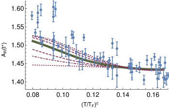
Figure 1: Aspect ratio $A_{r}$ as a function of the temperature $T/T_{F}$ in units of the Fermi temperature at the center of the trap. The data show $A_{R}$ at $t^{*}=1.2\times 10^{-3}$s after release from the trap Joseph:2014 . The lines show the prediction of viscous hydrodynamics for different values of the dimensionless parameter $\alpha=(0,0.5,1,2,3,4,5)$ (from bottom to top) defined in equ. (43). The thick green line corresponds to $\alpha=2$.

In our previous work we analyzed the data above $T_{c}$ assuming an expansion of the viscosity in the dimensionless diluteness $n\lambda^{3}$ of the gas, $\eta(n,T)\simeq\eta_{\it vir}(n,T)$ with

$$\eta_{\it vir}(n,T)=\eta_{0}(mT)^{3/2}\left\{1+\eta_{2}\left(n\lambda^{3}\right)+\eta_{3}\left(n\lambda^{3}\right)^{2}+\ldots\right\}.$$ (41)

Here, $\lambda=[2\pi/(mT)]^{1/2}$ is the thermal de Broglie wavelength. In Bluhm:2017rnf we obtained

$$\eta_{0}=0.265\pm 0.02\,,\hskip 28.45274pt\eta_{2}=0.060\pm 0.02\,.$$ (42)

We also found that $\eta_{3}$ is consistent with zero. Note that $\eta_{0}$ can be compared to the kinetic theory result $\eta_{0}=15/(32\sqrt{\pi})\simeq 0.264$ Bruun:2005 . Here, we will study whether the data constrain the behavior below $T_{c}$. We consider the parametrization

$$\eta(n,T<T_{c}(n))=\eta_{\it vir}(n,T)\exp\left(\alpha\left[1-\frac{T_{c}(n)}{T}\right]\right),$$ (43)

where $\alpha$ is a parameter that governs the low temperature behavior of the viscosity and $T_{c}(n)\simeq 0.167(3)T_{F}(n)$ is the critical temperature for the superfluid transition. This parametrization is sufficiently flexible to accommodate the main possible behaviors of the shear viscosity at low temperature. For $\alpha>0$ the viscosity tends to zero as $T\to 0$, for $\alpha\simeq 0$ the viscosity is approximately constant, and for $\alpha<0$ the viscosity diverges as $T\to 0$. We should note that the data mainly constrain the viscosity in the regime $0.5\mathrel{\hbox to0.0pt{\lower 4.0pt\hbox{$\sim$}\hss}\raise 1.0pt\hbox{$<$}}(T/T_{c})\mathrel{\hbox to0.0pt{\lower 4.0pt\hbox{$\sim$}\hss}\raise 1.0pt\hbox{$<$}}1.0$, and that the value of $\alpha$ extracted from our analysis should not be taken as a quantitative prediction for the shear viscosity at very low temperature, $(T/T_{c})\mathrel{\hbox to0.0pt{\lower 4.0pt\hbox{$\sim$}\hss}\raise 1.0pt\hbox{$<$}}0.5$.

We analyze the data in the superfluid regime using the results from the previous section. As a first approximation we will solve the equation using the equation of state in the superfluid regime, but assume that the normal and superfluid velocities are equal, $\vec{v}_{n}\simeq\vec{v}_{s}\equiv\vec{v}$. We will then check this assumption by computing $\vec{w}=\vec{v}_{n}-\vec{v}_{s}$ using equ. (40). We use the equation of state and the initial state described in App. C and D. The equations of fluid dynamics are solved using the anisotropic fluid dynamics method described in Bluhm:2017rnf ; Bluhm:2015raa .

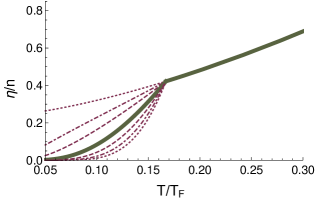
Figure 2: Viscosity to density ratio $\eta/n$ as a function of $T/T_{F}$, where $T_{F}$ is the local Fermi temperature. The lines show the fit obtained in this work, for different values of the parameter $\alpha$. The lines are labeled as in Fig. 1. In particular, the thick line corresponds to $\alpha=2$.

The results are shown in Fig. 1. We plot the data for $A_{R}(t^{*})$ as a function of the initial central temperature $T/T_{F}$ of the cloud. Note that he critical temperature is $T_{c}/T_{F}=0.167(3)$. We also remark that in a trap, the superfluid initially appears in the center of cloud, and that near $T_{c}$ the size of the superfluid core is small (see App. D for an illustration of the superfluid and normal density profiles). As a consequence, we observe that in the regime $T/T_{c}\in[0.8,1.0]$ the aspect ratio is only very weakly dependent on the viscosity in the superfluid. The data show a noticeable change in slope of $A_{R}$ as a function of $T/T_{F}$ at lower temperatures, $T\mathrel{\hbox to0.0pt{\lower 4.0pt\hbox{$\sim$}\hss}\raise 1.0pt\hbox{$<$}}0.8T_{c}$. We find that a good description of the data in this regime can only be achieved if the viscosity at low temperature drops below the extrapolation from the normal phase. It is difficult to fully quantify this statement, because the data contain some outliers, and the hydrodynamic prediction for $A_{R}(t^{*})$ is only weakly sensitive to the value of $\alpha$ beyond $\alpha\simeq 5$. Based on Fig. 1 we conclude that the data prefer $\alpha\mathrel{\hbox to0.0pt{\lower 4.0pt\hbox{$\sim$}\hss}\raise 1.0pt\hbox{$>$}}2$ (the prediction for $\alpha=2$ is shown as the thick green line in the figure).

The corresponding behavior of $\eta/n$ as a function of $T/T_{F}$ is shown in Fig. 2. We observe that the viscosity exhibits a fairly steep drop below the critical temperature. This behavior is in agreement with the reconstruction performed as part of the original experimental work Joseph:2014 . These authors find $\eta(0.8T_{c})=(0.32\pm 0.22)\eta(T_{c})$, compared to $\eta(0.8T_{c})\simeq 0.53\,\eta(T_{c})$ from Fig. 2. The analysis in Joseph:2014 is based on a number of simplifying assumptions. It assumes, in particular, that there is a critical radial distance in the expanding beyond which the cloud becomes free streaming. This radius is adjusted to reproduce the theoretically known value of the shear viscosity at large temperature Bruun:2005 . In our work the transitions to free streaming happens dynamically, governed by an extended hydrodynamic description that has been tested by comparison with exact numerical simulations of the Boltzmann equation Bluhm:2017rnf ; Pantel:2014jfa .

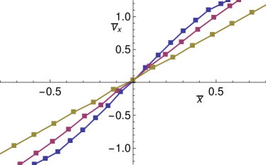
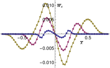
Figure 3: Perturbative estimate of the superfluid velocity $\vec{w}=\vec{v}_{n}-\vec{v}_{s}$. The left panel shows the average velocity in the $x$-direction $v_{x}\simeq(v_{n})_{x}\simeq(v_{s})_{x}$ from a simulation of trapped gas with central temperature $(T/T_{F})=0.094$. The position $\bar{x}=x/x_{0}$ and velocity $\bar{v}=v/v_{0}$ are given in dimensionless units, see App. D. The curves correspond to three different times $t=(0.25,0.50,0.75)\bar{\omega}^{-1}$ (blue, red, brown). The right panel shows the perturbative solution for $w_{x}$, as explained in the text. Note that the scale in the right panel is two orders of magnitude smaller.

Finally, we can go beyond earlier work and test the consistency of the assumption that the normal and superfluid velocities are equal. For this purpose we solve equ. (40) on the fluid dynamic background of the expanding solution with $\vec{w}=0$. The viscous heating rate is given by equ. (16,19)

$$\dot{\cal E}=\frac{\eta}{2}\left(\sigma_{ij}\right)^{2}\,,$$ (44)

where $\sigma_{ij}$ is the strain tensor defined in equ. (15). If the the viscosity is small then the velocity is approximately linear in distance, and $\sigma_{ij}$ is spatially constant. This implies that spatial gradients in the rate of energy dissipation are mostly governed by the functional form of the shear viscosity. Note that a possible non-zero $\zeta_{3}$ does not contribute to energy dissipation in the limit $\vec{w}\to 0$.

The change in temperature is given by $\dot{T}=\dot{\cal E}/c_{V}$, where $c_{V}$ is the specific heat, see App. C. Note that $c_{V}$ drops rapidly as $T/T_{F}\to 0$, so that the spatial structure of the temperature profile is very sensitive to rate at which $\eta$ and $c_{V}$ approach their low temperature values. The equation of motion for $\vec{w}$ also involves the ratio $s/\rho_{n}=s/(mn_{n})$. Both the numerator and the denominator vanish in the limit $T\to 0$, but for the unitary Fermi gas the ratio is $s/n_{n}$ close to unity and only weakly dependent on temperature, as shown in App. C. A numerical solution of equ. (40) is shown in Fig. 3. We observe that spatial variations in dissipative heating do indeed generate a second sound-like perturbation. We note, however, that the amplitude of this perturbation is smaller than the mean fluid velocity by almost two orders of magnitude. This means that the approximation $\vec{w}=0$ is consistent.

VII Summary and Outlook

In this work we have summarized the formalism for applying superfluid hydrodynamics to the dilute Fermi gas at unitarity, and constructed a suitable equation of state. We have showed that, unless the viscosity is very large, the equations can be solved perturbatively in the variable $\vec{w}=\vec{v}_{n}-\vec{v}_{s}$. We have numerically studied the evolution of a trapped Fermi gas after release from a deformed trap in the regime where the core of the cloud is superfluid. Comparing our simulations to the experimental data obtained in Joseph:2014 we conclude that the viscosity must drop significantly below $T_{c}$. This drop can be parametrized as an exponential decrease proportional to $\exp(-\alpha(T_{c}/T))$, where $\alpha\mathrel{\hbox to0.0pt{\lower 4.0pt\hbox{$\sim$}\hss}\raise 1.0pt\hbox{$>$}}2$.

Our results are in some tension with the data obtained in Patel:2019 . Patel et al. measure the sound attenuation in a unitary Fermi gas confined in a box trap at approximately constant density and different temperatures, both above and below $T_{c}$. They find that the sound diffusivity is approximately constant around $T_{c}$, and does not exhibit a pronounced decrease. The sound attenuation constant involves several transport coefficients, including the shear viscosity, the thermal conductivity, and, below $T_{c}$, the bulk viscosity coefficient $\zeta_{3}$. These transport coefficient can be disentangled using linear response measurements, as demonstrated in Baird:2019 , but this analysis has not been performed below $T_{c}$. This implies that it is possible that the sound diffusivity remains constant despite the fact that the viscosity is decreasing, but this behavior appears unlikely, and is not predicted by any transport theory analysis available in the literature.

It seems more plausible that the difference is explained by differences in the experimental approach. For example, it is possible that the viscosity of the superfluid phase is governed by a fairly dilute gas of quasi-particles, whereas transport in the normal phase is controlled by a system of dense, strongly correlated, excitations. In this case the superfluid core of an expanding gas cloud might be too small to exhibit dissipative two-fluid dynamics. This option can be addressed by studying linear response in a box trap, and we plan to extend our analysis to these systems in the future. The breakdown of superfluid dissipative hydrodynamics is observed in the collective mode experiments Patel:2019 . Dissipative fluid dynamics predicts that sound wave damping scales as wave number squared. This is seen over a wide range of wave numbers above $T_{c}$, but only in a much narrower window below $T_{c}$.

The work of J. H. and T. S. was supported in part by the US Department of Energy grant DE-FG02-03ER41260. We thank J. Thomas and M. Zwierlein for many useful discussions, and for providing us with the data published in Ku:2011 and Joseph:2014 .

Appendix A Galilean transformations

Under a Galilean transformation with boost velocity $\vec{u}$ we have

$$\rho^{\prime} = \rho\,,$$ (45)

$${\cal E}^{\prime} = {\cal E}+\vec{\jmath}\cdot\vec{u}+\frac{1}{2}\rho u^{2}\,,$$ (46)

$$\jmath^{\prime}_{i} = \jmath_{i}+\rho u_{i}\,,$$ (47)

$$Q_{i}^{\prime} = Q_{i}+u_{j}\Pi_{ij}+\frac{1}{2}u^{2}\jmath_{i}+{\cal E}^{\prime}u_{i}\,,$$ (48)

$$\Pi_{ij}^{\prime} = \Pi_{ij}+u_{i}\jmath_{j}+u_{j}\jmath_{i}+u_{i}u_{j}\rho\,,$$ (49)

where $\rho$ is the mass density, ${\cal E}$ is the energy density, $\vec{\jmath}$ is the mass current (momentum density), $\vec{Q}$ is the energy current, and $\Pi_{ij}$ is the stress tensor. The pressure and the entropy density of the fluid are Galilean invariant

$$P^{\prime}=P,\hskip 28.45274pts^{\prime}=s\,.$$ (50)

In a superfluid the normal and superfluid densities are separately Galilean invariant. The fluid velocities transforms as

$$\vec{v}_{\alpha}^{\,\prime}=\vec{v}_{\alpha}+\vec{u}\,,$$ (51)

where $\alpha=(n,s)$.

Appendix B Superfluid hydrodynamics in the normal fluid rest frame

In Section II we studied the thermodynamics of a moving superfluid by constructing the energy density in the superfluid rest frame. This procedure is well defined, even in the limit $T\to T_{c}$. However, one may be concerned that this method is not the best choice in the limit that the superfluid density is much smaller than the total density of the fluid. In this appendix we consider an alternative approach based on thermodynamic identities in the rest frame of the normal fluid. Consider the total energy density of a superfluid. Following Ho:1998 we write

$$d{\cal E}=\mu_{\jmath}dn+Tds+\vec{v}_{n}\cdot d\vec{\jmath}+\vec{\jmath}_{n}\cdot d\vec{v}_{s}\,.$$ (52)

which defines $\vec{v}_{n}$ and $\vec{\jmath}_{n}$ as variables conjugate to the momentum density $\vec{\jmath}$ and the superfluid velocity $\vec{v}_{s}$. We use the notation $\mu_{\jmath}$ to indicate that the chemical potential is defined at fixed $\vec{\jmath}$. Using Galilean invariance, ref. Ho:1998 shows that $\vec{\jmath}_{n}=\vec{\jmath}-\rho\vec{v}_{n}$, so that $\vec{\jmath}_{n}$ is the current in the normal fluid rest frame. We can also write $\vec{\jmath}=\rho_{n}\vec{v}_{n}+\rho_{s}\vec{v}_{s}$, so that $\vec{\jmath}_{n}=\rho_{s}(\vec{v}_{s}-\vec{v}_{n})\equiv-\rho_{s}\vec{w}$. We obtain the pressure by performing a Legendre transformation,

$$P=-{\cal E}+\mu_{\jmath}n+Ts+\vec{v}_{n}\cdot\vec{\jmath}$$ (53)

so that

$$dP=nd\mu_{\jmath}+sdT+\vec{\jmath}\cdot d\vec{v}_{n}-\vec{\jmath}_{n}\cdot d\vec{v}_{s}\,.$$ (54)

Using the explicit form of the currents in terms of the normal and superfluid densities as well as velocities we find the Gibbs-Duhem relation

$$dP=n\,d\mu_{n}+s\,dT-\frac{\rho_{s}}{2}dw^{2}\,,$$ (55)

where we have defined the chemical potential in the normal fluid frame

$$\mu_{n}=\mu_{\jmath}+\frac{1}{2}mv_{n}^{2}\,.$$ (56)

This Gibbs-Duhem relation implies that the superfluid density can be defined as

$$\rho_{s}=-2\left.\frac{\partial P}{\partial w^{2}}\right|_{\mu_{n},T}$$ (57)

This result should be compared with equ. (9). We note that the dependence of $P$ on $\vec{w}$ depends crucially on what chemical potential, $\mu_{n}$ or $\mu_{s}$, is held constant. The energy density in the normal fluid frame can be obtained via a Galilei transformation. We have

$${\cal E}_{n}={\cal E}-\vec{\jmath}\cdot\vec{v}_{n}+\frac{1}{2}\rho v_{n}^{2}$$ (58)

which implies that the pressure can be written as

$$P=-{\cal E}_{n}+\mu_{n}n+Ts\,.$$ (59)

Note that in the normal fluid frame we have the usual (one-fluid) relation $P+{\cal E}_{n}=\mu_{n}n+sT$.

In a scale invariant Fermi gas we can write

$$P(\mu_{n},T,\vec{w})=m^{3/2}\mu_{n}^{5/2}F_{n}\left(\frac{T}{\mu_{n}},\frac{mw^{2}}{\mu_{n}}\right)\,.$$ (60)

As before, we can try to simplify the problem by expanding the pressure in $\vec{w}$,

$$P(\mu_{n},T,\vec{w})=m^{3/2}\mu_{n}^{5/2}p_{n0}\left(\frac{T}{\mu_{n}}\right)-m^{5/2}\mu_{n}^{3/2}w^{2}p_{n1}\left(\frac{T}{\mu_{n}}\right)\,.$$ (61)

In the limit $\vec{w}\to 0$ this function must agree with equ. (25) so that $p_{n0}(s)=p_{s0}(x)=p(x)$. The second function $p_{n1}(x)$ determines the superfluid mass density

$$\rho_{s}=2m^{5/2}\mu_{0}^{3/2}p_{n1}\left(\frac{T}{\mu_{n}}\right).$$ (62)

which has been measured in Grimm:2013 ; Patel:2019 . Note that $\rho_{s}$ is positive, so the term proportional to $w^{2}$ lowers the pressure at fixed $\mu_{n}$ and $T$. The energy density in the normal fluid rest frame can be determined using

$${\cal E}_{n}=\left\{\mu_{n}\frac{\partial}{\partial\mu_{n}}+T\frac{\partial}{\partial T}-1\right\}P$$ (63)

where $P(\mu_{n},T,w)$ is given in equ. (61) above. At $O(w^{2})$ we find that

$$P=\frac{2}{3}{\cal E}_{n}-\frac{1}{3}\rho_{s}w^{2}\,.$$ (64)

At this order we also find that

$$P=\frac{2}{3}\left\{{\cal E}-\frac{1}{2}\rho_{n}v_{n}^{2}-\frac{1}{2}\rho_{s}v_{s}^{2}\right\}\,.$$ (65)

Like the results in Sect. II the expressions in equ. (64) and (65) are not given in terms of the primary variables $({\cal E},\rho,\vec{\jmath},\vec{v}_{s})$, and the equation of state is needed to determine $\rho_{n},\rho_{s}$ and $\vec{v}_{n}$. This can be accomplished by tabulating the equation of state, or by solving for $\rho_{s}$ iteratively in $\vec{w}$.

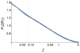
Figure 4: Pressure $P(\zeta)$ as a function of inverse fugacity $\zeta=\exp(-\mu/T)$ in units of the pressure $P_{F}$ of a free Fermi gas. The blue dots show the data taken by the MIT group. The solid line is our parametrization, which has a discontinuity at $\zeta=\zeta_{c}=0.082$.

Appendix C Equation of state

In this appendix we describe a parametrization of the equation of state of the unitary Fermi gas. We follow the basic strategy described in App. B of Bluhm:2017rnf , but we extend the method to the regime below the critical temperature. We begin by considering the pressure of a Fermi gas at rest. We write the pressure as

$$P(T,\mu)=T\lambda^{-3}f(\zeta)\,,$$ (66)

where $\lambda=[2\pi/(mT)]^{1/2}$ is the thermal de Broglie wave length, and $\zeta=exp(-\mu/T)$ is the inverse fugacity. In the regime above the critical temperature $T_{c}$ it is useful to represent the function $f(\zeta)$ in terms of the result for a free Fermi gas

$$f(\zeta)=h(\zeta)p_{F}(\zeta),\quad p_{F}(T,\mu)=-Li_{5/2}(-\zeta^{-1}).$$ (67)

The function $h(\zeta)$ was measured in Ku:2011 , see Fig. 4 We follow our previous work and parametrize $h(\zeta)$ in the normal fluid regime by a Pade approximant

$$\frac{h(\zeta)}{2}=\frac{\zeta^{2}+c_{1}\zeta+c_{2}}{\zeta^{2}+c_{3}\zeta+c_{4}},\hskip 28.45274pt\left(\zeta>\zeta_{c}=0.082\right)$$ (68)

with

$$c_{1}=1.32109,\quad c_{2}=0.026341,\quad c_{3}=0.541993,\quad c_{4}=0.005660.$$ (69)

Here, $\zeta_{c}=0.082$ is the critical value of the inverse fugacity obtained in Ku:2011 . Once the pressure is given, other thermodynamic observables are easily determined. We can write the density and entropy density as

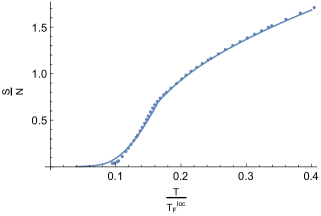
Figure 5: Entropy per particle $S/N$ as a function of temperature in units of Fermi temperature $T/T_{F}$. Here, $T_{F}$ is the local Fermi temperature of the gas, defined by $k_{B}T_{F}=k_{F}^{2}/(2m)$ and $k_{F}^{3}=3\pi^{2}n$. The data points are from Ku:2011 .

$$n(\mu,T)=\lambda^{-3}g(\zeta)\,,\hskip 14.22636pts(\mu,T)=\lambda^{-3}k(\zeta)\,.$$ (70)

where

$$g(\zeta) = -Li_{3/2}(-\zeta^{-1})h(\zeta)+\zeta Li_{5/2}(-\zeta^{-1})h^{\prime}(\zeta)\,,$$ (71)

$$k(\zeta) = -\left(\log(\zeta){\it Li}_{3/2}(-\zeta^{-1})+\frac{5}{2}{\it Li}_{5/2}(-\zeta^{-1})\right)h(\zeta)+\zeta\log(\zeta){\it Li}_{5/2}(-\zeta^{-1})h^{\prime}(\zeta)\,.$$ (72)

Other thermodynamic functions can be computed by taking additional derivatives. For example, the specific heat is given by

$$c_{V}=\frac{T}{V}\left.\frac{\partial S}{\partial T}\right|_{V}=T\left[\left.\frac{\partial s}{\partial T}\right|_{\mu}-\frac{[(\partial n/\partial T)|_{\mu}]^{2}}{(\partial n/\partial\mu)|_{T}}\right]\,.$$ (73)

The parametrization in equ. (68) is quite accurate, even at temperatures below $T_{c}$. However, $T=T_{c}$ is a genuine critical point and the parametrization should exhibit a non-analyticity at $\zeta=\zeta_{c}$. Furthermore, equ. (68) does not very accurately describe derivatives of the pressure in the regime $\zeta<\zeta_{c}$. In particular, the entropy density is unphysical for small values of $\zeta$.

In order to address these issues we employ a separate fit of the pressure in the regime $\zeta<\zeta_{c}$. We have chosen a physically motivated model of the pressure which is of the form

$$P(\mu,T)=\frac{2^{3/2}\mu^{5/2}m^{3/2}}{15\pi^{2}\xi^{3/2}}+\frac{\pi^{2}T^{4}}{90}\left(\frac{3m}{2\mu}\right)^{3/2}+A\mu^{5/2}m^{3/2}\sqrt{\frac{T}{\mu}}e^{-\frac{\mu B}{T}}.$$ (74)

Here, the first term is the zero temperature pressure expressed in terms of the Bertsch parameter $\xi=0.376$. The second term is the contribution of phonons in the superfluid phase, see, for example, ref. Braby:2010ec . The third term takes into account thermally excited fermionic quasi-particles, where $A$ and $B$ are treated as fit parameters. The structure of this term is taken from mean field calculations of the pressure in the BCS limit, see Gorkov . We fix the values of $A$ and $B$ by requiring the pressure and density to be continuous (but not differentiable) at $\zeta=\zeta_{c}$. This procedure ensures that the entropy density is continuous as well. We obtain

$$A=4.6699,\quad\quad\quad B=2.15436.$$ (75)

Note that we have not attempted to reproduce the exact critical behavior of the equation of state, which are expected to be those of the three dimensional $O(2)$ model. In a harmonic trap, the critical region is only a narrow shell in coordinate space, and critical behavior is difficult to observe.

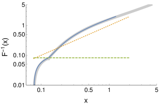
Figure 6: This plot shows the function $\zeta=F^{-1}(x)$ that determines the inverse fugacity in terms of a dimensionless ratio of the pressure and the density, $x\sim(mP)^{3/2}/n^{5/2}$. The solid blue line shows the two-component fit to the pressure and density. The dashed horizontal line is $\zeta_{c}=0.082$ and orange dotted line is the high temperature limit $F^{-1}(x)\simeq x$. The grey band is a fit to $F^{-1}(x)$ described in the text.

In terms of the functions $f(\zeta)$ and $g(\zeta)$ defined in equ. (66) and (70) the low temperature model of the equation of state is

$$f_{s}(\zeta) = \frac{2^{5/2}(2\pi)^{3/2}}{15\pi^{2}\xi^{3/2}}\left(-\log(\zeta)\right)^{5/2}+\frac{\pi^{2}(2\pi)^{3/2}}{90}\left(\frac{3}{2}\right)^{3/2}\left(-\log(\zeta)\right)^{-3/2}$$ (76)

$$\mbox{}+A(2\pi)^{3/2}\left(\log(\zeta)\right)^{2}\zeta^{B}$$

$$g_{s}(\zeta) = \frac{2^{5/2}(2\pi)^{3/2}}{6\pi^{2}\xi^{3/2}}\left(-\log(\zeta)\right)^{3/2}-\frac{\pi^{2}(2\pi)^{3/2}}{90}\left(\frac{3}{2}\right)^{5/2}\left(-\log(\zeta)\right)^{-5/2}$$ (77)

$$\mbox{}-A(2\pi)^{3/2}\left(2+B\log(\zeta)\right)\log(\zeta)\zeta^{B}$$

where $f_{s}(\zeta)=f(\zeta<\zeta_{c})$ and $g_{s}(\zeta)=g(\zeta<\zeta_{c})$. Equ. (66-68) and (76) define our equation of state. To illustrate the accuracy of this parametrization we show in Fig. 4 the pressure as a function of $\zeta$ and in Fig. 5 the entropy per particle as a function of $T/T_{F}$, both compared to the experimental results of the MIT group.

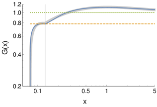
Figure 7: Temperature correction factor $G(x)=P/(nT)$ as a function of the dimensionless variable $x\sim(mP)^{3/2}/n^{5/2}$. The solid blue line shows the two-component fit to the pressure and density. The short dashed horizontal line is the high temperature limit $G=1$, and the long dashed line shows the critical value $G_{c}$. The grey band is a fit to $G(x)$ described in the text.

In fluid dynamics we have to reconstruct $\zeta$ from the density and pressure of the gas. For this purpose we consider the function

$$F(\zeta)=\frac{2f(\zeta)^{3/2}}{g(\zeta)^{5/2}},$$ (78)

where $f(\zeta)$ and $g(\zeta)$ are defined piecewise for $\zeta$ larger and smaller than $\zeta_{c}$. The function $F(\zeta)$ is proportional to the dimensionless ratio $(mP)^{3/2}/n^{5/2}$. We have

$$\zeta=F^{-1}\left(\frac{2}{(2\pi)^{3/2}}\frac{(mP)^{3/2}}{n^{5/2}}\right).$$ (79)

The function $F(\zeta)$ is defined so that $F(\zeta\gg\zeta_{c})\simeq\zeta$, and as a result $F^{-1}(x\gg x_{c})\simeq x$. We show $F^{-1}(x)$ for all $x$ in Fig. 6. Note that there is a minimum value of $x$, given by $x_{0}=F(0)$. In practice, we employ parametrization of $F^{-1}(x)$. This function is also defined piecewise for $x>x_{c}$ (corresponding to $T>T_{c}$) and $x<x_{c}$ (the regime $T<T_{c}$), where $x_{c}=0.1285$. For $x>x_{c}$ we again use a Pade approximant

$$F^{-1}_{\it fit}(x)=x\,\frac{1+h_{1}/x+h_{2}/x^{2}}{1+h_{3}/x+h_{4}/x^{2}},\hskip 28.45274pt\left(x>x_{c}=0.1285\right)$$ (80)

with

$$h_{1}=1.1601\,,\quad h_{2}=-0.0927\,,\quad h_{3}=0.2119\,,\quad h_{4}=0.07729\,.$$ (81)

In the superfluid regime $x<x_{c}$ we write

$$F^{-1}_{\it fit}(x)=\zeta_{c}^{\it fit}\left\{1-\left(\frac{x_{c}-x}{x_{c}-x_{0}}\right)^{3/2}\right\}^{2/3}$$ (82)

with

$$\zeta_{c}^{\it fit}=0.07732\,,\quad x_{c}=0.1285\,,\quad x_{0}=0.0775\,.$$ (83)

The function $F^{-1}(x)$ together with the fit given above is shown in Fig. 6.

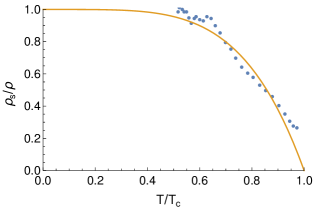
Figure 8: Superfluid mass fraction $\rho_{s}/\rho$ as a function of the temperature $T$ in units of the local Fermi temperature $T_{F}$. The points show the data from Grimm:2013 , and the line shows the fit discussed in the text. Note that the data points have uncertainties of order 10%, both in $T/T_{F}$ and $\rho_{s}/\rho$, that are not shown here.

Finally, given the local fugacity we have to determine the temperature and chemical potential of the fluid. In the high temperature limit this is straightforward; we can use $T=P/n$. In the general case we can write

$$T=G(x)\frac{P}{n}\,,$$ (84)

where $G(x)$ is a correction factor, given by

$$G(x)=\frac{g(\zeta(x))}{f(\zeta(x))}=\frac{g(F^{-1}(x))}{f(F^{-1}(x))}\,.$$ (85)

The function $G(x)$ extracted from our parametrization of the pressure and density is shown in Fig. 7. We note that for $x>x_{c}$ the function $G(x)$ is close to the high temperature limit $G=1$. In the low temperature regime $x<x_{c}$ the correction factor $G(x)$ drops very steeply, with $G(x_{0})=0$ at $x_{0}=0.0775$. This behavior motivates a simple two-component fit, similar to the one for $F^{-1}(x)$. We write

$$G_{\it fit}(x)=\frac{1+d_{1}/x+d_{2}/x^{2}}{1+d_{3}/x+d_{4}/x^{2}},\hskip 28.45274pt\left(x>x_{c}=0.1285\right)$$ (86)

with

$$d_{1}=1.8052\,,\quad d_{2}=-0.0022\,,\quad d_{3}=1.3668\,,\quad d_{4}=0.1179\,.$$ (87)

In the superfluid regime $x<x_{c}$ we write

$$G_{\it fit}(x)=G_{c}^{\it fit}\left\{1-\left(\frac{x_{c}-x}{x_{c}-x_{0}}\right)^{4}\right\}^{1/4}\,.$$ (88)

with $G_{c}^{\it fit}=0.7944.$

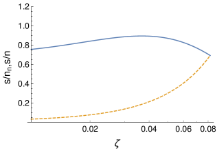
Figure 9: Entropy density over superfluid density (solid line), and entropy density over total density (dashed line) in the superfluid regime, plotted as a function of the inverse fugacity $\zeta$.

As explained in the text, in the superfluid phase there is an additional thermodynamic function, the superfluid mass density $\rho_{s}(\mu,T)$. The superfluid mass fraction was determined in Grimm:2013 , see also the recent work Patel:2019 . We show the results of Grimm:2013 in Fig. 8. A simple quasi-particle model for these results is discussed by Baym and Pethick Baym:2013 . Here we use an even simpler parametrization, given by

$$\frac{\rho_{s}}{\rho}=1-\left(\frac{T}{T_{c}}\right)^{9/2}\,,$$ (89)

where $T_{c}$ is the critical temperature. This parametrization is not directly motivated by a physical model, but numerically close to the theory of Baym and Pethick. Note that the superfluid density of a dilute Bose gas scales as $\rho_{s}/\rho=1-(T/T_{c})^{3/2}$. Finally, based on this result we can compute the ratio of the entropy density over the normal fluid density, which enters in the equation for the acceleration of $\vec{w}$, see equ. (40). The result is shown in Fig. 9.

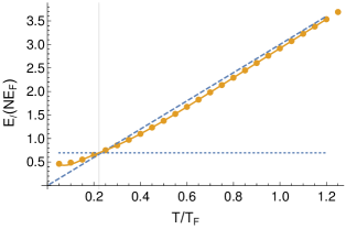
Figure 10: Energy versus temperature for a harmonically trapped Fermi gas. The energy is given in units of $NE^{\it trap}_{F}$, where $E^{\it trap}_{F}=3N^{1/3}\bar{\omega}$. The temperature is given in units of $T^{\it trap}_{F}=E^{\it trap}_{F}$ (where $k_{B}=1$). The points are computed from our parametrization of the equation of state, the dotted line is an interpolating function. The dashed diagonal line corresponds to the high temperature limit $E=(3/2)T$. The horizontal and vertical lines indicate the critical values $T_{c}/T^{\it trap}_{F}=0.222$ and $E_{c}/E^{\it trap}_{F}=0.695$.

Appendix D Trapped Fermi gas

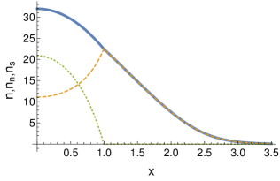
Figure 11: Density profile of a harmonically trapped Fermi gas below the critical temperature at which superfluidity appears at the center of the trap. We show the total (blue), normal (yellow, dashed), and superfluid (green, dotted) densities $n,n_{n}$ and $n_{s}$ in units of $\lambda^{-3}$ as a function of $x$ in units of the length $x_{0}$ defined in the text. Here, the central inverse fugacity was chosen as $\zeta_{0}=0.05$.

A trapped Fermi gas in thermal equilibrium is a solution of the hydrostatic equation. As explained in Sect. V in both the normal and the superfluid regime the solution is given by

$$n(\vec{x},t)=n(\mu_{s}(\vec{x}),T)\,\hskip 28.45274pt\mu_{s}(\vec{x})=\mu_{c}-V_{\it ext}(\vec{x})\,.$$ (90)

In the experiment we consider trapped clouds with a given number of particles $N$ at a fixed temperature $T$ or total energy $E$. Given $N$ and $T$ the central inverse fugacity $\zeta_{0}=\zeta(0)$ is fixed by the condition

$$\frac{3}{(2\pi)^{3}}\left(\frac{T}{T^{\it trap}_{F}}\right)\int d^{3}x\,g\left(\zeta_{0}\exp\left(\frac{x^{2}}{2}\right)\right)\equiv 1\,,$$ (91)

where $T^{\it trap}_{F}=3N^{1/3}\bar{\omega}$ is the Fermi temperature of the trap. Once $\zeta_{0}$ is determined the total energy can be computed using the virial theorem. Making use of the virial theorem we can calculate the energy of the trapped gas

$$\frac{E}{NE^{\it trap}_{F}}=\left(\frac{T}{T^{\it trap}_{F}}\right)^{3}\frac{\int d^{3}x\,x^{2}g\left(\zeta_{0}\exp\left(\frac{x^{2}}{2}\right)\right)}{\int d^{3}x\,g\left(\zeta_{0}\exp\left(\frac{x^{2}}{2}\right)\right)}\,.$$ (92)

Fig. 10 shows $E/(NE^{\it trap}_{F})$ as a function of $T/T^{\it trap}_{F}$ for a harmonically trapped Fermi gas. The critical temperature and energy, that means the value of $T$ and $E$ at which superfluidity appears at the center of the trap, are

$$T_{c}/T^{\it trap}_{F}=0.222\,,\quad E_{c}/(NE^{\it trap}_{F})=0.695$$ (93)

The zero temperature limit of the energy is $E_{0}/(NE^{\it trap}_{F})=(3\sqrt{\xi})/4=0.460$.

An example for the density profile of a harmonically trapped Fermi gas in the superfluid regime is shown in Fig. 11. In this example the inverse fugacity at the trap center is $\zeta_{0}=0.05$, corresponding to a central temperature $T/T_{F}=0.13$. We note that there is a two-fluid mixture in the core. The superfluid appears at some critical radius $x_{c}$, but the total density only shows a very mild non-analyticity at $x_{c}$. In the figure the position $x$ is shown in dimensionless units $\bar{x}=x/x_{0}$ with

$$x_{0}=\left[\frac{2}{3}\frac{(3N)^{1/3}}{m\bar{\omega}}\right]^{1/2}\,.$$ (94)

Similar dimensionless can be employed for time $\bar{t}=t/t_{0}$ with $t_{0}=\bar{\omega}^{-1}$ and velocity $\bar{v}=v/v_{0}$ with $v_{0}=t_{0}/x_{0}$. In our hydrodynamic simulations we also use dimensionless variables for thermodynamic quantities, such as density $\bar{n}=n/n_{0}$, pressure $\bar{P}=P/P_{0}$, temperature $\bar{T}=T/T_{0}$, and viscosity $\bar{\eta}=\eta/\eta_{0}$

$$n_{0}=x_{0}^{-3},\quad P_{0}=m\bar{\omega}^{2}x_{0}^{-1},\quad T_{0}=m\bar{\omega}^{2}x_{0}^{2},\quad\eta_{0}=m\bar{\omega}x_{0}^{-1}.$$ (95)

References

- (1) I. Bloch, J. Dalibard, W. Zwerger, “Many-Body Physics with Ultracold Gases” Rev. Mod. Phys. 80, 885 (2008) [arXiv:0704.3011].
- (2) S. Giorgini, L. P. Pitaevskii, S. Stringari, “Theory of ultracold atomic Fermi gases” Rev. Mod. Phys. 80 1215 (2008) [arXiv:0706.3360].
- (3) M. J. H. Ku, A. T. Sommer, L. W. Cheuk, and M. W. Zwierlein, “Revealing the Superfluid Lambda Transition in the Universal Thermodynamics of a Unitary Fermi Gas,” Science 335, 563 (2012) [arXiv:1110.3309 [cond-mat.quant-gas]].
- (4) T. Schäfer and D. Teaney, “Nearly Perfect Fluidity: From Cold Atomic Gases to Hot Quark Gluon Plasmas,” Rept. Prog. Phys. 72, 126001 (2009) [arXiv:0904.3107 [hep-ph]].
- (5) A. Adams, L. D. Carr, T. Schäfer, P. Steinberg and J. E. Thomas, “Strongly Correlated Quantum Fluids: Ultracold Quantum Gases, Quantum Chromodynamic Plasmas, and Holographic Duality,” New J. Phys. 14, 115009 (2012) [arXiv:1205.5180 [hep-th]].
- (6) T. Schäfer, “Fluid Dynamics and Viscosity in Strongly Correlated Fluids,” Ann. Rev. Nucl. Part. Sci. 64, 125 (2014) [arXiv:1403.0653 [hep-ph]].
- (7) T. Schäfer, “The Shear Viscosity to Entropy Density Ratio of Trapped Fermions in the Unitarity Limit,” Phys. Rev. A 76, 063618 (2007) [arXiv:cond-mat/0701251].
- (8) A. Turlapov, J. Kinast, B. Clancy, L. Luo, J. Joseph, J. E. Thomas, “Is a Gas of Strongly Interacting Atomic Fermions a Nearly Perfect Fluid” J. Low Temp. Phys. 150, 567 (2008) [arXiv:0707.2574].
- (9) K. M. O’Hara, S. L. Hemmer, M. E. Gehm, S. R. Granade, J. E. Thomas, “Observation of a Strongly-Interacting Degenerate Fermi Gas of Atoms,” Science Vol. 298, No. 5601, 2179 (2002). [cond-mat/0212463].
- (10) M. Bluhm and T. Schäfer, “Model-independent determination of the shear viscosity of a trapped unitary Fermi gas: Application to high temperature data,” Phys. Rev. Lett. 116, no.11, 115301 (2016) [arXiv:1512.00862 [cond-mat.quant-gas]].
- (11) M. Bluhm, J. Hou and T. Schäfer, “Determination of the density and temperature dependence of the shear viscosity of a unitary Fermi gas based on hydrodynamic flow,” Phys. Rev. Lett. 119, no. 6, 065302 (2017) [arXiv:1704.03720 [cond-mat.quant-gas]].
- (12) T. Enss, R. Haussmann and W. Zwerger, “Viscosity and scale invariance in the unitary Fermi gas,” Annals Phys. 326, 770 (2011) [arXiv:1008.0007 [cond-mat.quant-gas]].
- (13) J. Hofmann, “Current response, structure factor and hydrodynamic quantities of a two- and three-dimensional Fermi gas from the operator product expansion,” Phys. Rev. A 84, 043603 (2011) [arXiv:1106.6035 [cond-mat.quant-gas]].
- (14) J. Hofmann, “High-temperature expansion of the viscosity in interacting quantum gases,” Phys. Rev. A 101, no.1, 013620 (2020) doi:10.1103/PhysRevA.101.013620 [arXiv:1905.05133 [cond-mat.quant-gas]].
- (15) B. Frank, W. Zwerger and T. Enss, “Quantum critical thermal transport in the unitary Fermi gas,” Phys. Rev. Res. 2, no.2, 023301 (2020) [arXiv:2003.10338 [cond-mat.quant-gas]].
- (16) J. A. Joseph, E. Elliott, J. E. Thomas, “Shear viscosity of a universal Fermi gas near the superfluid phase transition,” Phys. Rev. Lett. 115, 020401 (2015) [arXiv:1410.4835 [cond-mat.quant-gas]].
- (17) G. Rupak and T. Schäfer, “Shear viscosity of a superfluid Fermi gas in the unitarity limit,” Phys. Rev. A 76, 053607 (2007) [arXiv:0707.1520 [cond-mat.other]].
- (18) H. Guo, D. Wulin, C.-C. Chien, K. Levin, “Perfect Fluids and Bad Metals: Transport Analogies Between Ultracold Fermi Gases and High Superconductors,” New J. Phys. 13, 075011 (2011) [arXiv:1009.4678 [cond-mat.supr-con]].
- (19) G. Wlazlowski, P. Magierski, A. Bulgac and K. J. Roche, “The temperature evolution of the shear viscosity in a unitary Fermi gas,” Phys. Rev. A 88, 013639 (2013) [arXiv:1304.2283 [cond-mat.quant-gas]].
- (20) P. Patel, Z. Yan, B. Mukherjee, R. Fletcher, J. Struck, M. Zwierlein, “Universal Sound Diffusion in a Strongly Interacting Fermi Gas”, preprint (2019) [arXiv:1909.02555 [cond-mat.quant-gas]].
- (21) D. Vollhardt, P. Wolfle, “The Superfluid Phases of Helium 3”, Taylor and Francis (1990).
- (22) L. D. Landau, E. M. Lifshitz, “Fluid Mechanics,” Course of Theoretical Physics, Vol. 6, Pergamon (1984).
- (23) D. T. Son, “Vanishing bulk viscosities and conformal invariance of unitary Fermi gas,” Phys. Rev. Lett. 98, 020604 (2007) [arXiv:cond-mat/0511721 [cond-mat]].
- (24) E. Zaremba, T. Nikuni, A. Griffin, “Dynamics of trapped Bose gases at finite temperatures,” J. Low Temp. Phys. 116, 227 (1999) [arXiv:cond-mat/9903029 [cond-mat.stat-mech]].
- (25) Y.-H. Hou, L. P. Pitaevskii, S. Stringari, “Scaling solutions of the two-fluid hydrodynamic equations in a harmonically trapped gas at unitarity,” Phys. Rev. A. 87, 033620 (2013) [arXiv:1302.2258 [cond-mat.quant-gas]].
- (26) T. Schäfer and C. Chafin, “Scaling Flows and Dissipation in the Dilute Fermi Gas at Unitarity,” Lect. Notes Phys. 836, 375-406 (2012) [arXiv:0912.4236 [cond-mat.quant-gas]].
- (27) T. Schäfer, “Dissipative fluid dynamics for the dilute Fermi gas at unitarity: Free expansion and rotation,” Phys. Rev. A 82, 063629 (2010) [arXiv:1008.3876 [cond-mat.quant-gas]].
- (28) G. M. Bruun, H. Smith, “Viscosity and thermal relaxation for a resonantly interacting Fermi gas”, Phys. Rev. A 72, 043605 (2005) [cond-mat/0504734].
- (29) M. Bluhm and T. Schäfer, “Dissipative fluid dynamics for the dilute Fermi gas at unitarity: Anisotropic fluid dynamics,” Phys. Rev. A 92, vol. 4, 043602 (2015) [arXiv:1505.00846 [cond-mat.quant-gas]].
- (30) P. A. Pantel, D. Davesne and M. Urban, “Numerical solution of the Boltzmann equation for trapped Fermi gases with in-medium effects,” Phys. Rev. A 91, 013627 (2015) [arXiv:1412.3641 [cond-mat.quant-gas]].
- (31) L. Baird, X. Wang, S. Roof, and J. E. Thomas, J “Measuring the Hydrodynamic Linear Response of a Unitary Fermi Gas,” Phys. Rev. Lett. 123, 160402 (2019) arXiv:1906.11179 [cond-mat.quant-gas].
- (32) T.-L. Ho, V. B. Shenoy, “The hydrodynamic equations of superfluid mixtures in magnetic traps,” J. Low. Temp. Phys. 111, 937 (1998).
- (33) L. Sidorenkov, M. Tey, R. Grimm, L. Pitaevski, S. Stringari, “Second sound and the superfluid fraction in a Fermi gas with resonant interactions,” Nature 498, 78-81 (2013) [arXiv:1302.2871 [cond-mat.quant-gas]].
- (34) M. Braby, J. Chao and T. Schäfer, “Thermal Conductivity and Sound Attenuation in Dilute Atomic Fermi Gases,” Phys. Rev. A 82, 033619 (2010) [arXiv:1003.2601 [cond-mat.quant-gas]].
- (35) A. A. Abrikosov, L. P. Gorkov, I. E. Dzyaloshinski, “Methods of Quantum Field Theory in Statistical Physics,” Dover Publications (1963).
- (36) G. Baym, C. J. Pethick, “Normal mass density of a superfluid Fermi gas at unitarity,” Phys. Rev. A 88, 043631 (2013) [arXiv:1308.3812 [cond-mat.quant-gas]].