A Hybrid Decomposition-based Multi-objective Evolutionary Algorithm for the Multi-Point Dynamic Aggregation Problem

Abstract

An emerging optimisation problem from the real-world applications, named the multi-point dynamic aggregation (MPDA) problem, has become one of the active research topics of the multi-robot system. This paper focuses on a multi-objective MPDA problem which is to design an execution plan of the robots to minimise the number of robots and the maximal completion time of all the tasks. The strongly-coupled relationships among robots and tasks, the redundancy of the MPDA encoding, and the variable-size decision space of the MO-MPDA problem posed extra challenges for addressing the problem effectively. To address the above issues, we develop a hybrid decomposition-based multi-objective evolutionary algorithm (HDMOEA) using $\varepsilon$-constraint method. It selects the maximal completion time of all tasks as the main objective, and converted the other objective into constraints. HDMOEA decomposes a MO-MPDA problem into a series of scalar constrained optimization subproblems by assigning each subproblem with an upper bound robot number. All the subproblems are optimized simultaneously with the transferring knowledge from other subproblems. Besides, we develop a hybrid population initialisation mechanism to enhance the quality of initial solutions, and a reproduction mechanism to transmit effective information and tackle the encoding redundancy. Experimental results show that the proposed HDMOEA method significantly outperforms the state-of-the-art methods in terms of several most-used metrics.

I Introduction

What is the MDPA problem, why is the MPDA problem is important The Multi-Point Dynamic Aggregation (MPDA) problem is a task planning problem of the multi-robot system, which comes from the real world [1, 2, 3, 4, 5]. Recently, it has become one of the active research topics due to its applications such as bushfire elimination routing, search and rescue, and medical resource scheduling domains [6, 7, 8]. Unlike the majority of scheduling and routing problems [9, 10, 11, 12], the demand of each task in the MPDA problem increase over time, Besides, all the robots can execute one task simultaneously to promote the efficacy of completing the task. The traditional objective of the MPDA problem is to design execution plans for all the robots to execute geographically distributed tasks in order to minimise the makespan (the completion time of the last completed task).

The previous researchers did not consider the MO-MPDA problem, we focus on the MO-MPDA problem The previous researches about the MDPA problem only focused on the single objective problem [13, 14, 15]. However, when the MPDA problem is applied to solve the real-world applications, it always has two or more objectives that are usually conflicted. Thus, in this paper, we focus on the multi-objective MPDA (MO-MPDA) problem with two objectives. In the MO-MPDA problem, there is a number of tasks (e.g. fire points) with time-varying demands in the workspace. One objective is to minimise the cost of using robots, and the cost is considered as the number of the robots in this paper. The other objective is to complete all the tasks as soon as possible, and it is considered as the maximal completion time of all the tasks (makespan).

There are some challenges in the MO-MPDA problem. First, due to the multi-objective characteristic, the previous single-objective MPDA optimisation approaches [15, 16, 3] cannot efficiently handle the two conflict objectives. When the number of used robots is changed, the whole single-objective approach needs to be adjusted to satisfy the changing robot number. Second, in the MO-MPDA problem, the length of the routing plan for one robot is not fixed, and the number of used robots is not fixed. Compared with the traditional multiobjective optimization problems with the fixed-length decision variables, the MO-MPDA is difficult to solve due to their variable-length Pareto structure, where the number of variables in two different Pareto solutions might not be identical in the decision space. Third, the used robots are homogeneous so that there are many isomorphic execution plans for these robots. The fitness landscape of the MO-MPDA problem is so flat that some changes on the execution plan may not have ant effect on the objective value. Last but not least, the time-varying demand and collaboration between robots lead the MO-MPDA problem has a large search space, in which an effective solution is non-trivial to be found.

Introduce the MOEA/D method. MOEA/D was first introduced in 2007 [17], and it shown very promising results for approximating the Pareto front. Decomposition is the main idea for the MOEA/D method, it decomposes a multi-objective problem into a number of scalar optimisation subproblems. Each subproblem learning valid information from its neighbouring subproblems so that all the subproblems are evolved collaboratively. Thank to the decomposition mechanism, the MOEA/D method has a relative low computational cost. Meanwhile, the MOEA/D method has a good population diversity due to the a scalar of the weight vectors in the objective space. There have been a variety of MOEA/D method with some promising results [18, 19, 20]. To the best of our knowledge, there is no previous work that has been applied MOEA/D to the MO-MPDA problem.

Introduce the DMOEA-$\varepsilon$C method. The $\varepsilon$-constraint method is firstly proposed in [21], which selects one objective as the main objective and converts the other objectives into constraints [22]. The decomposition-based multi-objective evolutionary algorithm with the $\varepsilon$-constraint framework (DMOEA-$\varepsilon$C) [23] firstly combined the $\varepsilon$-constraint method and MOEA/D method to address the multi-objective problem. In DMOEA-$\varepsilon$C, a multi-objective problem is decomposed into several constrained optimization subproblems with different upper bounds. These constrained optimization subproblems are optimised collaboratively using the neighbour information. DMOEA-$\varepsilon$C is a very competitive MOEA method, and it has shown obvious advantages over MOEA/D on combinational optimisation problem [23, 24, 19, 25]. Since the MPDA problem is a constraint combinational optimisation problem, we expect DMOEA-$\varepsilon$C to be effective in addressing the MO-MPDA problem.

When we apply DMOEA-$\varepsilon$ to address the MO-MPDA problem, some issues need to be solved. First, there is no existing mathematical model which can characterise the MO-MPDA problem. Second, the traditional solution-to-subproblem mechanism and subproblem-to-solution mechanism are difficult to be used in the MO-MPDA problem. Third, the random initialisation mechanism cannot generate high-quality solutions, even cannot generate feasible solutions for some tight-constraints scenarios. Finally, it is challenging to tackle the encoding redundancy caused by homogeneous robots.

To address the above issues, we establish a MO-MPDA model and design a hybrid DMOEA-$\varepsilon$C (HDMOEA-$\varepsilon$C) method. Specifically, the contributions of this paper are shown as follows.

• We formulate a MO-MPDA problem with two correlated objectives. One of the objectives is to minimise the cost of using robots ( the number of robots), and the other objective is to minimise the maximum completion time of all the tasks.

• According to the characteristics of the MO-MPDA problem, we design a novel HDMOEA-$\varepsilon$C method including the designed solution-to-subproblem mechanism and subproblem-to-solution mechanism.

• A hybrid initialisation strategy of the proposed HDMOEA-$\varepsilon$C method is designed to produce a fraction of high-quality initial solutions. In the initialisation strategy, a heuristic method considering the travelling cost, completion time, and the incremental rate of tasks generate a solution for each number of robots, the other solutions are generated by a random method.

• In the designed reproduction strategy used in the reproduction process of HDMOEA-$\varepsilon$C, all visiting sequences of all robots are first sorted according to the number of visiting tasks and the index of tasks. Then, a mutation operator and three crossover operators are used to reproduction new solutions in order to effective information transmission.

The rest of this paper is organised as follows. The related work and mathematical model of the MO-MPDA problem are presented in Section II. Then, Section III proposed the HDMOEA-$\varepsilon$C method. Section IV presents the experimental results and performance analysis of the proposed mechanisms. Finally, this paper is concluded in Section V.

II Background

In this section, the related work about MPDA and MOEA is introduced first, and then the problem formulation of the MO-MPDA problem is given.

II-A Related Work

II-A1 Multi-Point Dynamic Aggregation

Introduce the MPDA problem The MPDA problem is a novel optimisation problem that originates from the multi-robot system, and its objective is to design an optimal execution plan to maximise the performance of the multi-robot system [26, 27, 2, 28]. In the MPDA problem, each task has a time-varying demand, which grows over time. A set of robots is located at a depot and sent to execute these tasks collaboratively. The MPDA problem can be applied to many real applications with time-varying demands and coordination behaviours (e.g. fire-fighting and area search). Due to the complex relationships among robots and tasks caused by the time-varying demand and coordinated execution, the MPDA problem is a very challenging and interesting problem. Over the past few years, researchers proposed several methods to address the MPDA problem [29, 13, 3].

There are several heuristic approaches proposed to address the MPDA problem. A real fire-fighting system with a UAV and a UGV was implemented in [29] by a simple heuristic approaches. The UAV in the fire-fighting system was used for the detection to reduce the uncertain of tasks, and the UGV was used to execute and complete the tasks. Teng et al. [15] modified the bid value based-on the auction mechanism of the multi-robot system, considering robots’ characteristics and the task’s completion requirement. Du et al. [13] proposed a recruitment strategy to address the MPDA problem. In the proposed recruitment method, when a robot is not able to complete its executing task, the robots will recruit some robots to completion the task together. Chen et al. [8] proposed a task assignment approach based on the completion time of each task. First, the task assignment approach tries to ensure every task is assigned to enough robots to complete it. Then, the approach assigns robots to the task with the largest reduction of the total completion time.

There are several meta-heuristic approaches proposed to address the MPDA problem. Although an execution plan of all the robots can be obtained by the aforementioned heuristic methods, the plan is not of a high quality due to the NP-hardness characteristic of the MPDA problem. Hence, several meta-heuristic approaches were proposed by researchers [30, 31, 14]. A task planning approach hybridised with a greedy method and a simulated annealing algorithm is proposed by Poggenpohl et al. [30]. The experimental results showed that the hybrid approach can lead to a better makespan and a better balance among the workloads of the robots. Another hybrid method combining differential evolution and estimation of distribution algorithm was proposed to address the MPDA planning problem by [31]. The experimental results showed that the hybrid method [31] outperforms the differential evolution in terms of the convergence speed and solution quality. A multi-model estimation of distribution algorithm with a multi-permutation encoding method was designed in [14]. The experimental results showed that the method [14] outperforms the genetic algorithm and random search method. An adaptive coordination ant colony optimisation with an individual learning strategy is proposed to address the MPDA problem [16]. Experiments showed that the proposed ant colony optimisation algorithm significantly achieved a better performance than the state-of-the-art algorithms.

II-A2 Decomposition based Multi-objective Evolutionary Algorithms

Decomposition based MOEA has attracted great attention in recent years thanks to its decomposition and parallelism characteristics, and has become one of the mainstream methods to solve a multi-objective problem [32, 33, 34]. MOEA/D [17] is the most popular one. MOEA/D decomposes a multi-objective optimisation problem into a series of single objective subproblems by using scalar aggregation functions (such as weighted sum, Tchebycheff and PBI) and a set of uniformly distributed weights, and uses EA to optimize all subproblems. MOEA/D defines the neighborhood relationship between subproblems according to the Euclidean distance between weight vectors. When solving each subproblem, only the information of its neighborhood subproblem is used, which makes MOEA/D have low computational complexity. Besides, MOEA/D implicitly guarantees the diversity of the population in the target space by giving a group of well-distributed weights. In recent years, many scholars have improved MOEA/D, mainly including the following aspects: weight design and adjustment, adding new search engines to the original MOEA/D framework, proposing new aggregation functions, and using MOEA/D and its improved forms to solve various types of real-world problems.

Scholars have proposed variants of MOEA/D to promote performance. MOEA/D with dynamic resource allocation [35] adjusts the computing resources allocated to each subproblem dynamically. MOEA/D with adaptive weight adjustment [36] proposes a new weight generation method based on the analysis of the geometric relationship between the weight vector of Tchebycheff scalar function and the optimal solution of a corresponding scalar function. Ishibuchi et al. [45] demonstrated that employing a local replacement neighborhood structure is very important for the performance of MOEA/D. Wang et al. proposed a global replacement scheme that assigns a new solution to its most suitable subproblems. Meanwhile, in the method, a dynamic adjusting replacement method of the neighborhood size was developed to promote the efficacy. Zhou et al. [37] extended the dynamic resource adjustment strategy in[35] to generalized resource allocation. The method [37] allocates an improved probability vector for each subproblem, and allocates computing resources for each subproblem according to the improved probability vector. Chen et al. proposed MOEA/D which decomposes a multi-objective problem to several $\varepsilon$-constraint optimization subproblem, which of the details are shown as follows.

$$\begin{array}[]{l}\begin{array}[]{*{20}{c}}{{\mathop{\rm minimize}}}\nolimits&{{f_{main}}={f_{s}}({\bf{x}})}\end{array}+\rho\sum\limits_{i=1}^{m}{{f_{i}}({\bf{x}})}\\ {\rm{~{}~{}subject~{}to}}\left\{\begin{array}[]{l}\frac{{{f_{i}}({\bf{x}})-z_{i}^{*}}}{{z_{i}^{nad}-z_{i}^{*}}}\leq{\varepsilon_{i}},\forall i\in\{1,2,\cdots,m\}/\{s\}\\ {\bf{x}}=({x_{1}},{x_{2}},...,{x_{n}})\in\Omega\end{array}\right.\end{array}$$ (1)

where $s$ represents the predefined main objective index, $0\leq{\bf{\varepsilon}}=({\varepsilon_{1}},...,{\varepsilon_{s-1}},{\varepsilon_{s+1}},...,{\varepsilon_{m}})\leq 1$ is the upper bound vector, $\rho$ is a small positive number, ${{\bf{z}}^{\bf{*}}}=(z_{1}^{*},...,z_{m}^{*})$ and ${{\bf{z}}^{{\bf{nad}}}}=(z_{1}^{nad},...,z_{m}^{nad})$are the ideal point and the nadir point, respectively. An example of the $\varepsilon$-constraint method with different upper bounds is shown in Fig. 1. $f_{1}$ in Fig. 1 is chosen as the main objective to be minimised, and a series of upper bounds is applied into $f_{2}$. The black points represent the Pareto optimal solution within the given upper bounds vectors.

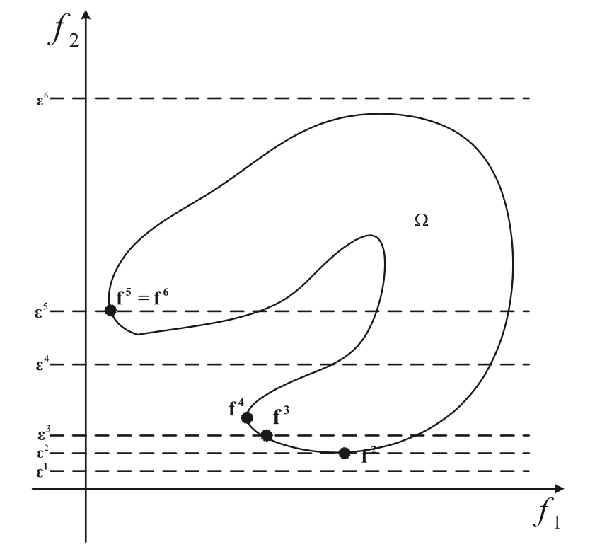
Figure 1: An example of the $\varepsilon$-constraint method with different upper bounds.

II-B Problem Formulation

There is a number of tasks (e.g. fire points) with time-varying demands in the MO-MDPA problem. The decision maker wants to design a execution plan which completes all the tasks as soon as possible with as few robots as possible We use an undirected graph $G(\mathcal{V,E})$ to define the MO-MPDA problem. In the set of vertexes $\mathcal{V}=\{v_{0},v_{1},\dots,v_{N}\}$ of $G$, $v_{0}$ indicates the depot, and $\{v_{1},\dots,v_{N}\}$ indicates the set of tasks. Each task $v_{i}$ has an inherent time-varying demand $q_{i}(t)$, which is changed based on the following equation

$$q_{i}(t)=q_{i}(0)+\alpha_{i}\times t,$$ (2)

where $\alpha_{i}$ represents the inherent increment rate of task $v_{i}$. In the set of edges of $G$, every edge indicates a route among two tasks with the travel time $t_{ij}$.

Several homogeneous robots located at the depot are going to execute all the tasks. Every robot has the same ability $\beta$, representing the amount of demand which it can reduce per time unit. Fig. 2 shows an example demonstrating the relationship between the task demand and abilities of robots. In Fig. 2, the inherent increment rate $\alpha_{i}$ of the exampled task is 3, and the ability of a robot is 1.5. $rob_{1}$, $rob_{2}$ and $rob_{3}$ arrive at the task at time 2, 4 and 6 respectively. After $rob_{1}$ arrives, the current incremental rate of the task is 3 - 1.5 = 1.5. After $rob_{2}$ reaches the task, the demand of the task is constant. At time 6, $rob_{3}$ arrives, and the total robot ability is greater than the inherent increment rate. Finally, the demand is decreased to 0, and the task is completed by these three robots.

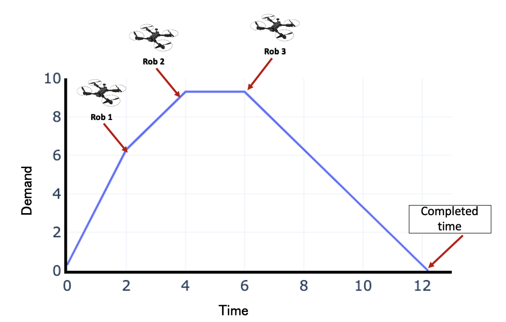
Figure 2: An example of the demand of an executed task over time.

Based on the aforementioned notations, the MO-MPDA model can be defined as follows.

$$\small f_{1}=\min\max_{i\in\{1,\cdots,N\}}ct_{i}$$ (3)

$$\small f_{2}=\min m$$ (4)

$$\small s.t.\sum_{j=0}^{N}x_{ij}^{k}=\sum_{j=0}^{N}x_{ji}^{k},\forall i=1,\dots,N,\forall k=1,\dots,m$$ (5)

$$\small\sum_{i=0}^{N}\sum_{k=1}^{m}x_{ij}^{k}\geq 1,\forall j=1,\dots,N$$ (6)

$$\small\sum_{i=0}^{N}x_{ij}^{k}\leq 1,\forall j=1,\dots,N,\forall k=1,\cdots,m$$ (7)

$$\small at_{0k}=ct_{0}=0,\forall k=1,\cdots,m$$ (8)

$$\small at_{jk}=\sum_{i=0}^{N}(ct_{i}+t_{ij})x_{ij}^{k},\forall j=1,\dots,N,\forall k=1,\cdots,m$$ (9)

$$\small q_{j}(0)+\alpha_{j}ct_{j}=\sum_{i=0}^{N}\sum_{k=1}^{m}x_{ij}^{k}\beta(ct_{j}-at_{jk}),\forall j=1,\dots,N$$ (10)

$$\small\alpha_{j}<\sum_{k=1}^{m}\sum_{i=0}^{N}x_{ij}^{k}\beta,\forall j=1,\dots,N$$ (11)

$$\small x_{ij}^{k}\in\{0,1\},i\neq j,\forall i,j=1,\dots,N,\forall k=1,\dots,m$$ (12)

where the integer decision variable $m$ represents the number of robots executing all the tasks, and the binary decision variables $x_{ij}^{k}$ takes 1 if $rob_{k}$ goes from $v_{i}$ to $v_{j}$, and 0 otherwise. $at_{jk}$ represents the arrival time of $rob_{k}$ at $v_{j}$, and $ct_{j}$ represents the completion time of $v_{j}$. The notations used in the problem formulation are summarised in Table I.

One objective (3) is to minimise the maximum completion time of all the tasks, and the other objective (4) is minimise the number of robots executing all the tasks. Constraint (5) indicates that the number of outgoing routes equals the number of incoming routes for each task and each robot. Constraint (6) ensures that each task is executed by at least one robot. Constraint (7) ensures that each task is executed by each robot at most once. Constraint (8) sets the arrival time and completion time for the depot to 0. Constraint (9) specifies the relationship between $ct_{j}$, $at_{jk}$ and $x^{k}_{ij}$. Constraint (10) implies that a task is completed when its demand decreases to zero (i.e. the accumulated demand from time 0 to $ct_{j}$ equals the total demand reduced by the robots executing the task during this time period). It also shows the time-varying characteristic of the task demand. Constraint (11) indicates that for each task, the total ability of the robots executing it must be greater than its inherent increment rate. Otherwise, the task can never be completed. Constraint (12) sets the binary domain of the decision variables.

TABLE I: The notations used in the paper

Notation	Description
$N$	the number of tasks
$v_{j}$	the task with index $j$
$q_{j}(t)$	the demand of $v_{j}$ accumulated at time $t$
$\alpha_{j}$	the inherent increment rate of $v_{j}$
$t_{ij}$	travel time from $v_{i}$ to $v_{j}$
$rob_{k}$	the robot with index $k$
$\beta$	the ability of a robot
$at_{jk}$	the arrival time of $rob_{k}$ at $v_{j}$
$ct_{j}$	the completion time of $v_{j}$
$x_{ij}^{k}$	1 if $rob_{k}$ goes from $v_{i}$ to $v_{j}$, and 0 otherwise

III The proposed HDMOEA-$\varepsilon$C algorithm

The framework of the proposed HDMOEA-$\varepsilon$C method is shown in Algorithm 1. HDMOEA-$\varepsilon$C contains four main components, 1) initialisation, 2) reproduction, 3) matching, and 4) Pareto updating. HDMOEA-$\varepsilon$C selects the maximal completion time of all the tasks as the main objective, and converts the number of using robots as the constraints. In the algorithm, $R$ upper bounds for the number of using robots are maintained for the evolutionary process, which is the same as the population size. At the beginning of HDMOEA-$\varepsilon$C, $R$ solutions are initialised based on the heuristic method and random method in the designed initialisation method. Then, the rest three components of HDMOEA-$\varepsilon$C are run iteratively until the number of fitness evaluations is large than the maximum number of fitness evaluations. In each generation of the proposed method, $I$ solution are selected to reproduce new solutions Y firstly. Second, for each solution of the new generated solutions Y, it is matched to a subproblem using the subproblem-to-solution matching method. Finally, the external archive $EP$ is updated according to the solutions of the current population.

Algorithm 1 The proposed HDMOEA-$\epsilon$C method

INPUT: A MO-MPDA instance, related parameters.

OUTPUT: An external archive population $EP$.

1:  Calculate the upper bound and low bound of the number of robots.

2:  Initialise $R$ evenly spread upper bound vectors, and initialise the evolving population $Pop=\{x^{1},\dots,x^{R}\}$ according to the spread upper bound vectors using Algorithm 2.

3:  Extract nondominated individuals from $Pop$ denoted as $EP$. $gen=0,n=N$

4:  for $i=1$ to $R$ do

5:     Set the neighbourhood of the $i$th subproblem, $\pi^{i}=1$.

6:  end for

7:  if  $gen$ is a multiple of $DRA\_interval$  then

8:     Update the indices of the subproblem $I$ that will be evolved in the next generations.

9:  end if

10:  while $n\leq NFE$ do

11:     for $i\in I$ do

12:        $P=\left\{\begin{array}[]{l}B(i),~{}~{}~{}~{}~{}~{}~{}~{}~{}~{}\text{if}~{}rand<\delta\\ \{1,2,...,R\},~{}\text{otherwise}\end{array}\right.$

13:        Reproduction (Algorithm 4): Select parent individuals from $P$ randomly and apply certain reproduction operator to generate new individuals Y.

14:        for $y\in\textbf{Y}$ do

15:           If a new individual $y$ is infeasible, repair it.

16:           Use the subproblem-to-solution matching method (Algorithm 5) to find subproblems K for the new solution $y$ .

17:           Compare $y$ with solutions of the subproblems K, and update solutions and neighbouring solutions of the subproblems K.

18:           Update the external archive $EP$.

19:        end for

20:     end for

21:     $gen=gen+1$

22:  end while

III-A Representation and Decoding Strategy

III-A1 Representation

The explicit representation of the execution plan of all the robots in the MPDA problem is a variable-length sequence of events. To simplify the representation, an implicit representation of a solution for the MO-MPDA problem is adopted in this paper, which is a matrix and shown in (13).

$$X=\left[{\begin{array}[]{*{20}{c}}\pi_{1,[1]}&\pi_{1,[2]}&\cdots&\pi_{1,[N]}\\ \pi_{2,[1]}&\pi_{2,[2]}&\cdots&\pi_{2,[N]}\\ \vdots&\vdots&\vdots&\vdots\\ \pi_{m,[1]}&\pi_{m,[2]}&\cdots&\pi_{m,[N]}\end{array}}\right]$$ (13)

The size of rows of the solution represents the number of robots using in the MO-MPDA problem. Each row of the given representation has $N$ integral elements which is a permutation of all tasks’ indexes. Similar to the representation in VRPs [38, 39], the elements of one row indicate the task-executing sequences. For example, if $i$th row is $[2,3,1]$, $rob_{i}$ will intend to execute tasks $v_{2}$, $v_{3}$ and $v_{1}$ in order.

III-A2 Decoding

The decoding method used in this paper adopts the event trigger mechanism. When a robot completed a task, it becomes active and selects its next executing task according to the corresponding encoding. The details of the decoding method can be found in [16, 3]. Fig. 3 shows an example of the decoding process of the MPDA problem with the given encoding. There are three robots and five tasks in the example, and each robot executes tasks in sequence according to the given encoding. Task $v_{5}$ which is executed by three robots simultaneously is the last completed task. Thus, for the MO-MPDA problem, the first objective of the example solution in Fig. 3 is the completion time of $v_{5}$, and the second objective is 3.

Remark: A robot will not visit all tasks according to the give encode. There may be some invalid elements in each row of the given encoding. The number of invalid elements in a row is denoted as $ie_{k}$ in this paper. For example, $ie_{3}$ of $rob_{3}$ is 3 in Fig. 3. It also should be noticed that many encoding representations have the same objective values since the abilities of robots are the same. For example, swapping the visiting sequences of $rob_{1}$ and $rob_{2}$ does not affect the objective values.

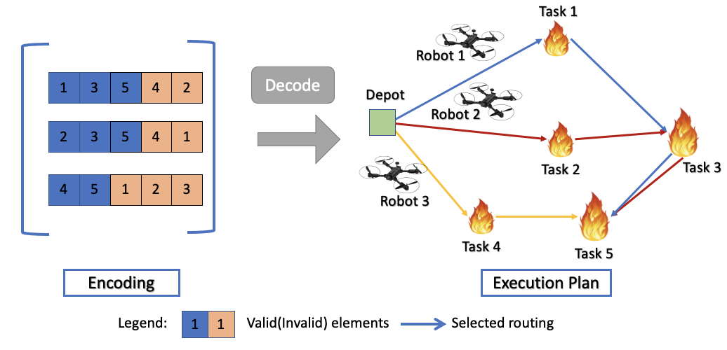
Figure 3: An example of decoding processes of the MPDA problem with the given encode.

III-B The designed Hybrid initialisation mechanism

III-B1 Bound determination

At the beginning of the designed hybrid initialisation mechanism, the low bound LBM and upper bound UBM of the number of used robots are calculated as shown in Eqs. (14) and (15).

$$\textbf{LBM}=\lceil\frac{\max_{i\in\{1,\cdots,R\}}\alpha_{i}}{\beta}\rceil$$ (14)

$$\textbf{UBM}=\sum_{i=1}^{N}\lceil\frac{\alpha_{i}}{\beta}\rceil+1$$ (15)

where LBM represents the minimal number of used robots which ensures every task can be completed, and UBM represents the maximal number of robots which ensures all the tasks can be executed by one assignment. Meanwhile, a series of scalar upper bounds ${\bf{\varepsilon}}=({\varepsilon_{1}},\varepsilon_{2},...,{\varepsilon_{R}})$ for the number of used robots are generated within an equal space $\bigtriangleup=1/(R-1)$. Thus, a subproblem $sp_{l}$ of HDMOEA-$\varepsilon$C is shown as following.

$$\begin{array}[]{l}\begin{array}[]{*{20}{c}}{{\mathop{\rm minimize}}}\nolimits&{{f_{main}}={f_{1}}({\bf{x}})}\end{array}\\ {\rm{~{}~{}subject~{}to}}\left\{\begin{array}[]{l}f_{2}\leq\varepsilon_{l}(\textbf{UBM}-\textbf{LBM})+\textbf{LBM}\\ {\bf{x}}\in\Omega\end{array}\right.\end{array}$$ (16)

It should be noticed that the objective of the robot number is always integer. It is also obvious that the robot number of the optimal solution x of $sp_{l}$ is $\lfloor\varepsilon_{l}(\textbf{UBM}-\textbf{LBM})+\textbf{LBM}\rfloor$.

III-B2 Population initialisation

Due to the complex relationships among robots and tasks of the MO-MPDA problem, a purely random initialisation cannot provide solutions of good-quality, even cannot generate feasible solutions. Conversely, an elaborate heuristic method is competent to find an acceptable solution at a small computational cost. Incorporating the random and heuristic initialisation methods, a hybrid initialization strategy shown in Algorithm 2 is developed to generate the initial population for each subproblem in the proposed HDMOEA-$\varepsilon$C method. For each subproblem, its solution is generated according to $m$ determined using robots (line 3 of Algorithm 2). For a specific determined number of using $m$ robots, the heuristic generation method shown in Algorithm 3 is preferred over the random solution generation method. Provided that the heuristic method has generated a solution for a specific $m$, the rest of the solutions based on $m$ robots are generated by the random method.

Algorithm 2 Hybrid initialisation strategy

INPUT: MO-MPDA instance $\Xi$.

OUTPUT: Initial population $Pop$.

1:  $Pop=\emptyset$, and $\mathcal{M}$

2:  for $l\rightarrow P$ do

3:     Calculate $\lfloor\varepsilon_{l}(\textbf{UBM}-\textbf{LBM})+\textbf{LBM}\rfloor$ as $m$.

4:     if $m\in\mathcal{M}$ then

5:        $sol$ = RandomGenerate($\Xi,m$)

6:     else

7:        $sol$ = HeuristicGenerate($\Xi,m$), and $\mathcal{M}$ = $\mathcal{M}\cup m$

8:     end if

9:     $Pop=Pop\cup sol$

10:  end for

Many factors including the travelling cost, increment rates of tasks and the number of using robots contribute to the complexity of the MO-MPDA problem. A greedy heuristic method considering one factor cannot generate good solutions for different instance with different characteristics. Thus, a comprehensive heuristic method considering the arrival time, completion time of robots and workload balance, is designed in this paper. The details of the designed heuristic method are shown in Algorithm 3. The heuristic method generates $2|\textbf{W}|$ solutions with different weights and sorting rules, the best performance solution $sol^{*}$ of $2|\textbf{W}|$ generated solutions are complemented and returned as the initial solution for the corresponding subproblem. The reason for the complementing process is that a robot may not visit all the tasks in the best performance solution $sol^{*}$. To keep the same encoding length, the rest tasks which are not assigned to the robot are shuffled and added to the end of the sequence. Provided that the sorting rule and weight $\omega$ are given, the inner loop of the heuristic algorithm adopt the event trigger mechanism. We divide the inner loop generation method into three stages: initialisation stage (line 4), decision-making stage (lines 6-25), and updating stage (line 26).

In the initialisation stage, the solution is set as empty, and the states of robots and tasks are initialised. When robots become active, they calculate the priorities of the candidate tasks in the set $\mathcal{T}^{(t)}$ according to the perdition arrival and completion time with the given sorting rule and $\omega$. To normalise the arrival and completion time of different tasks, the priorities of the candidate tasks is obtained by the weighted orders of the sorted arrival time AT and sorted completion time CT. When the boolean rb is 1, CT is sorted from small to large. Otherwise, CT is sorted from large to small. It should be noticed that the completion time rules. Each active robot selects the task with the highest priority to execute next. After that, the states of robots and tasks are updated by Algorithm StateUpdate, whose details can be found in [3, 16]. Meanwhile, Algorithm StateUpdate returns the new set of active robots for the next round of the decision-making process.

Algorithm 3 Heuristic Generation algorithm HeuristicGenerate($\Xi,m$)

INPUT: MO-MPDA instance $\Xi$, number of using robots $m$.

OUTPUT: Solution $sol^{*}$.

1:  A list of solutions LSOL, and generate a series weights W with the same space $\bigtriangleup$

2:  for rb $\in\{0,1\}$ do

3:     for $\omega\in\textbf{W}$ do

4:        Initialisation stage of the construction process, $sol=()$

5:        while There are uncompleted tasks do

6:           Get all uncompleted tasks $\mathcal{T}^{(t)}$, and $\Pi=\emptyset$.

7:           for $rob_{k}\in\mathbf{AR}$ do

8:              $\textbf{AT}=\emptyset$, $\textbf{CT}=\emptyset$.

9:              for $v_{i}\in\mathcal{T}^{(t)}$ do

10:                 Calculate prediction arrival time $at_{i}k$, prediction completion time $ct_{i}k$, and prediction incremental rate $\lambda_{i}(t)$.

11:                 $\textbf{AT}=\textbf{AT}\cup at_{i}k$

12:              end for

13:              Sort AT from small to large.

14:              if rb == 1 then

15:                 Sort CT from small to large.

16:              else

17:                 Sort CT from large to small.

18:              end if

19:              for $v_{i}\in\mathcal{T}^{(t)}$ do

20:                 Get the order of $v_{i}$ in AT and CT respectively, denoted as $\textbf{AT}_{[v_{i}]}$ and $\textbf{CT}_{[v_{i}]}$.

21:                 $p_{i}=\omega\textbf{AT}_{[v_{i}]}+(1-\omega)\textbf{CT}_{[v_{i}]}$.

22:              end for

23:              Assign $v_{k}^{*}=\arg\max_{i=1}^{|\varOmega|}p_{i}$ to $rob_{k}$.

24:           end for

25:           Set $\Pi={[rob_{k},v^{*}_{k}]|rob_{k}\in\mathbf{AR}}$.

26:           [$\mathbf{AR},sol$] = StateUpdate($\Pi,sol$)

27:        end while

28:        $\textbf{LSOL}=\textbf{LSOL}\cup sol$

29:     end for

30:  end for

31:  $sol^{*}=\arg\max_{i=1}^{|\textbf{LSOL}|}f_{1}(sol_{i})$, and complement $sol^{*}$.

III-C Reproduction strategy

The reproduction strategy is an important aspect of MOEAs, which generates new offspring solutions through transferring information among the parent solutions. And the reproduction process not only is expected to generate diversified solutions, but also is able to propagate excellent information from parents [40]. The representation of the MO-MPDA problem is multiple permutations of the tasks’ indexes, and previous researchers have developed a large number of crossover operators and mutation operators [41, 42]. Thus, we developed the reproduction strategy based on the classical crossover operator (partially matched crossover) and mutation operator (swap mutation) [43], which is shown in Algorithm 4. In the proposed reproduction strategy, there are two generation operators. When a sampled value less than $\delta_{g}$, the new offspring solutions are provided by the designed crossover operator. Otherwise, the new offspring solutions are generated by the designed mutation operator.

Since the robots in the MO-MPDA problem are homogeneous, the permutation encoding has great redundancy. At the beginning of the designed crossover operator, permutations in each parent solution are sorted according to the number of invalid elements and task indexes to address the redundancy issue. Then, the two situations are distinguished. The first situation is that parent solutions $X_{a}$ and $X_{b}$ have the same number of using robots. For each permutation of the parent solutions, the partially matched crossover generates offspring permutations to construct the new offspring solutions Y. When the parent solutions $X_{a}$ and $X_{b}$ have different numbers of using robots, the new offspring solutions Y are constructed by three parts. The first part of the new offspring solutions is similar to the previous situation, and it includes two generated solutions based on the partially matched crossover. The second part is based on the second part, and it includes up to 10 new solutions, which is constructed by selecting $f_{2}(Y_{a})$ permutations from the solution with a large number of robots $f_{2}(Y_{a})$ to construct new solutions. The last part is generated by inheriting the alleles from the two parent individuals with no implicit mutations.

Algorithm 4 Reproduction strategy Reproduce($X_{a}$, $X_{b}$)

INPUT: . Parents solution $X_{a}$ and $X_{b}$

OUTPUT: New offspring solutions Y.

1:  if  $rand<\delta_{g}$  then

2:     Sort $X_{a}$ and $X_{b}$ based on the number of invalid elements and task indexes from small to large.

3:     if $X_{a}$ and $X_{b}$ have the same number of using robots then

4:        for  $i\rightarrow f_{2}(X_{a})$ do

5:           The partially matched crossover operates $X_{a,i}$ and $X_{b,i}$ to generate offspring permutations $Y_{a,i}$ and $Y_{b,i}$.

6:        end for

7:        $\textbf{Y}=\{Y_{a},Y_{b}\}$.

8:     else

9:        for  $i\rightarrow\min\{f_{2}(X_{a}),f_{2}(X_{b})\}$ do

10:           The partially matched crossover operates $X_{a,i}$ and $X_{b,i}$ to generate offspring permutations $Y_{a,i}$ and $Y_{b,i}$.

11:        end for

12:        $\textbf{Y}=\{Y_{a},Y_{b}\}$.

13:        if $f_{2}(Y_{a})>f_{2}(Y_{b})$ then

14:           Swap $Y_{a}$ and $Y_{b}$.

15:        end if

16:        for $i\rightarrow\min\{\tbinom{f_{2}(Y_{a})}{f_{2}(Y_{b})},10\}$ do

17:           Select $f_{2}(Y_{a})$ permutations randomly of $Y_{b}$ to construct $Y_{c}$.

18:           $\textbf{Y}=\textbf{Y}\cup Y_{c}$

19:        end for

20:        for  $i\rightarrow\min\{f_{2}(X_{a}),f_{2}(X_{b})\}$ do

21:           Swap $X_{a,i}$ and $X_{b,i}$ to generate $Y_{a,i}$ and $Y_{b,i}$.

22:        end for

23:        $\textbf{Y}=\textbf{Y}\cup\{Y_{a},Y_{b}\}$.

24:     end if

25:  else

26:     Swap mutation operates each permutation of $X_{a}$ and $X_{b}$ to generate offspring $Y_{a}$ and $Y_{b}$.

27:     $\textbf{Y}=\{Y_{a},Y_{b}\}$.

28:  end if

III-D Subproblem-to-Solution

When a new solution is generated, it is necessary to determine which subproblem is suitable for the solution. To make the best use of information about the new generated solutions, we develop a subproblem-to-solution matching procedure, which is shown in Algorithm 5. In the matching procedure, the subproblem that does not violate constraints and has the maximal makespan objective is selected for the newly generated solution. Since the feasibility rule is adopted to handle constrained subproblems, this procedure is good for convergence. The solution-to-subproblem matching procedure and the subproblem-to-solution matching procedure consider diversity and convergence, respectively.

Algorithm 5 Subproblem-to-Solution Matching

INPUT: $N$ subproblems ${{\bf{\varepsilon}}^{1}}{\bf{,}}{{\bf{\varepsilon}}^{2}}...{\bf{,}}{{\bf{\varepsilon}}^{N}}$ and new generated solution ${\bf{y}}$. OUTPUT: The index of the selected subproblem $k$.

1:  for $i\rightarrow R$ do

2:     $C{V^{i}}=\min(\varepsilon_{i}-\frac{{f_{2}(\bf{y})-\textbf{LBM}}}{{\textbf{UBM}-\textbf{LBM}}},0)$

3:     if $C{V^{i}}\neq 0$ then

4:        $C{V^{i}}=f_{1}(sol_{i})$

5:     end if

6:  end for

7:  $k=\arg\max_{1,...,R}(CV^{1},...,CV^{R})$.

III-E Discussion

III-E1 Time Complexity Analysis

The proposed HDMOEA-$\epsilon$C method is used to optimise the MO-MPDA problem in which the number of tasks is $N$, and the upper bound of the robot number is UBM. In each iteration, there are $R$ solution in the population to evolve. Table II shows the time complexity of HDMOEA-$\epsilon$C. In the initialisation process, the time complexity mainly consists of the random and heuristic generation methods. In the evolutionary process, the time complexity mainly lies in the dynamic resource allocation, reproduction, subproblem-to-solution, updating $EP$, and decoding process. In summary, the time complexity of HDMOEA-$\epsilon$C is ${\rm{O}}(R(\textbf{UBM}\times N(N+\textbf{UBM}))+R^{2})$.

TABLE II: Time complexity of HDMOEA-$\epsilon$C.

Parameter	Value
Random solution generation	${\rm{O}}(\textbf{UBM}\times N)$
Heuristic solution generation	${\rm{O}}(\textbf{UBM}\times N(N+\textbf{UBM}))$
Dynamic resource allocation	${\rm{O}}(R)$
Reproduction process	${\rm{O}}(R\times N\times\textbf{UBM})$
Subproblem-to-solution matching	${\rm{O}}(R)$
Update $EP$	${\rm{O}}(R^{2})$
Decoding process	${\rm{O}}(\textbf{UBM}\times N(N+\textbf{UBM}))$

IV DESIGN OF EXPERIMENTS

IV-A Data Set

There is not existing benchmark set for the MO-MPDA problem. To fair compare performances of different algorithms on the MO-MPDA problem, a comprehensive MO-MPDA benchmark set is developed in this paper. Following the characteristics of MPDA problem and VRPs [16, 3, 44], we transformed the single-objective MPDA benchmark set to a MO-MDPA benchmark set. The settings of instances of the MO-MPDA problem including the number of tasks, task initial demands and inherent increment rates follows the settings of the most comprehensive MPDA benchmark set in [16]. The abilities of each robots of the designed MO-MPDA is set as the mean abilities of all robots in the MPDA benchmark set in [16]. Table III shows the full details of all the designed instances, and the instances are named by the number of tasks, the position of tasks, the abilities of robots, and the inherent increment rate of tasks .

TABLE III: Main characteristics of forty-five designed instances.

ID	name	$N$	PR	PT	$\beta$	$\alpha$
1	5_C_CL_2.86	5	C	CL	[0.02, 0.05]	[0.05, 0.15]
2	5_EC_RCL_2.86	5	EC	RCL	[0.02, 0.05]	[0.05, 0.15]
3	10_C_R_0.54	10	C	R	[0.05, 0.08]	[0.02, 0.05]
4	10_EC_CL_0.54	10	EC	CL	[0.05, 0.08]	[0.02, 0.05]
5	10_EC_RCL_1.86	10	EC	RCL	[0.02, 0.05]	[0.05, 0.08]
6	10_C_R_4.29	10	C	R	[0.02, 0.05]	[0.1, 0.2]
7	10_C_RCL_1.86	10	C	RCL	[0.02, 0.05]	[0.05, 0.08]
8	10_C_CL_1.0	10	C	CL	[0.05, 0.08]	[0.05, 0.08]
9	10_EC_RCL_1.86A	10	EC	RCL	[0.02, 0.05]	[0.05, 0.08]
10	10_C_CL_1.86	10	C	CL	[0.02, 0.05]	[0.05, 0.08]
11	10_C_R_1.86	10	C	R	[0.02, 0.05]	[0.05, 0.08]
12	10_C_CL_4.29	10	C	CL	[0.02, 0.05]	[0.1, 0.2]
13	10_EC_R_2.86	10	EC	R	[0.02, 0.05]	[0.05, 0.15]
14	15_EC_CL_1.0	15	EC	CL	[0.05, 0.08]	[0.05, 0.08]
15	15_EC_CL_1.0A	15	EC	CL	[0.02, 0.05]	[0.02, 0.05]
16	15_EC_CL_1.86	15	EC	CL	[0.02, 0.05]	[0.05, 0.08]
17	15_C_RCL_4.29	15	C	RCL	[0.02, 0.05]	[0.1, 0.2]
18	20_EC_R_1.0	20	EC	R	[0.05, 0.08]	[0.05, 0.08]
19	20_C_R_2.86	20	C	R	[0.02, 0.05]	[0.05, 0.15]
20	20_EC_CL_0.54	20	EC	CL	[0.05, 0.08]	[0.02, 0.05]
21	20_C_R_4.29	20	C	R	[0.02, 0.05]	[0.1, 0.2]
22	20_EC_R_0.54	20	EC	R	[0.05, 0.08]	[0.02, 0.05]
23	20_EC_RCL_1.0	20	EC	RCL	[0.05, 0.08]	[0.05, 0.08]
24	20_EC_RCL_2.86	20	EC	RCL	[0.02, 0.05]	[0.05, 0.15]
25	20_C_RCL_4.29	20	C	RCL	[0.02, 0.05]	[0.1, 0.2]
26	30_C_CL_1.0	30	C	CL	[0.02, 0.05]	[0.02, 0.05]
27	30_EC_R_1.0	30	EC	R	[0.02, 0.05]	[0.02, 0.05]
28	30_C_RCL_1.86	30	C	RCL	[0.02, 0.05]	[0.05, 0.08]
29	30_EC_CL_2.86	30	EC	CL	[0.02, 0.05]	[0.05, 0.15]
30	30_C_R_4.29	30	C	R	[0.02, 0.05]	[0.1, 0.2]
31	40_C_R_0.54	40	C	R	[0.05, 0.08]	[0.02, 0.05]
32	40_C_CL_1.86	40	C	CL	[0.02, 0.05]	[0.05, 0.08]
33	40_EC_CL_1.0	40	EC	CL	[0.02, 0.05]	[0.02, 0.05]
34	40_EC_R_1.86	40	EC	R	[0.02, 0.05]	[0.05, 0.08]
35	40_EC_R_4.29	40	EC	R	[0.02, 0.05]	[0.1, 0.2]
36	60_C_CL_1.0	60	C	CL	[0.02, 0.05]	[0.02, 0.05]
37	60_C_R_0.54	60	C	R	[0.05, 0.08]	[0.02, 0.05]
38	60_C_R_1.0	60	C	R	[0.05, 0.08]	[0.05, 0.08]
39	60_C_CL_1.0A	60	C	CL	[0.02, 0.05]	[0.02, 0.05]
40	60_C_R_1.0A	60	C	R	[0.02, 0.05]	[0.02, 0.05]
41	60_EC_R_1.0	60	EC	R	[0.02, 0.05]	[0.02, 0.05]
42	80_EC_CL_1.0	80	EC	CL	[0.02, 0.05]	[0.02, 0.05]
43	80_EC_CL_0.54	80	EC	CL	[0.05, 0.08]	[0.02, 0.05]
44	80_EC_R_0.54	80	EC	R	[0.05, 0.08]	[0.02, 0.05]
45	120_EC_RCL_1.0	120	EC	RCL	[0.05, 0.08]	[0.05, 0.08]

• PR means positions of robots, PT means positions of tasks, C represents central, E represent Eccentric, R represents random, CL represents Clustered, and RC represents Random-Clustered.

IV-B Competitor Algorithms

Since the MO-MPDA problem is a novel problem and no existing algorithms can be directly applied for comparison, we compare HDMOEA-$\varepsilon$C with the following baseline algorithms:

• NSGA-II [45]. It is one of the most popular MOEAs, selects individuals according to Pareto dominance relation and propagates offspring in an iterative way. The main feature of this algorithm is that it adopts the elitist nondominated sorting with the crowding distance as a ranking criterion.

• MOEA/D [17] and MOEA/D-DRA [35]. They are both developed according to the decomposition strategy and outperform a number of popular algorithms.

• MOEA/D-VLP [46]. The MO-MPDA problem is a variable-length multi-objective optimisation problem. MOEA/D-VLP is a state-of-the-art algorithm for the variable-length optimisation problem. In MOEA/D-VLP, it decomposes a multi-objective problem in terms of the penalty boundary intersection search directions and the dimensionality of variables.

• MOEA/D-ACO [47]. The adaptive ACO method proposed in [16] is a state-of-the-art algorithm for the single-objective MPDA problem. Following the ideas in [47], we combine the adaptive ACO method and MOEA/D to address the MO-MPDA problem.

IV-C Performance metrics and parameter settings

IV-C1 Performance metrics

Three commonly used performance metrics, i.e., inverted generational distance (IGD) [48] and hypervolume (HV) [49] are employed to evaluate the performance of all compared algorithms in this paper. IGD and HV assess the quality of a nondominated set in terms of convergence and diversity, and their definitions are shown in Eqs. (17) and (18).

$$IGD({P^{*}},P)=\frac{{\sum\nolimits_{{x^{*}}\in{P^{*}}}{d({x^{*}},P)}}}{{|{P^{*}}|}}$$ (17)

$$HV(P,{\bf{r}})=VOL(\bigcup\limits_{x\in P}{[{f_{1}}(x),{r_{1}}]\times...\times[{f_{m}}(x),{r_{m}}]})$$ (18)

where $P$ represents the solution set, $\bf{r}$ represents the reference point, and ${P^{*}}$ represents the true pareto front. However, the ture pareto front of the MO-MPDA problem is very difficult to obtained due to the complexity of the problem. In this paper, we approximate the true pareto front by selecting non-dominated solutions from all the compared and designed algorithms [50]. The IGD and HV values are calculated based on the normalised objectives of which the range is [0,1], the normalisation methods are shown in Eqs. (19) and (20).

$$ob1_{n}=\frac{\ln(\max_{i\in\{1,\cdots,N\}}ct_{i})-2\ln(10)}{6\ln(10)-2\ln(10)}$$ (19)

$$ob2_{n}=\frac{m-\textbf{LBM}}{\textbf{UBM}-\textbf{LBM}}$$ (20)

where $\max_{i\in\{1,\cdots,N\}}ct_{i}$ ($m$) represents the maximal completion (number of robots) objective value, and $ob1_{n}$ ($ob2_{n}$) represents the first (second) normalised objective value. The point (1.1, 1.1) is used as the reference point in this paper.

IV-C2 Parameter settings

All the competitor algorithms and HDMOEA-$\epsilon$C for the MO-MPDA problem are implemented based on a Python evolutionary computation framework [51] to keep fair comparisons. The parameter settings of the proposed DMOEA-$\epsilon$C method used in the rest of this paper follow the conventional settings [17, 23, 19]. The detailed parameter setting are shown Table IV. For each instance, all the algorithms was run 20 times independently.

TABLE IV: Parameter settings of DMOEA-$\epsilon$C.

Parameter	Value
Pop Size $N$	100
Neighbourhood size $T$	$\lfloor 0.1N\rfloor$
Probability $\delta$	0.9
$DRA\_interval$	50
Selected subproblem size $|I|$	$\lfloor N/5\rfloor-2$
Stop criterion	$NFE$ = 50000
Weight size $|\textbf{W}|$	11
Mutation probability $\delta_{g}$	0.9

V RESULTS AND DISCUSSIONS

First, HDMOEA-$\epsilon$C is compared with the state-of-the-art MOEAs on the benchmark set of the MO-MPDA problem. Then, further analyses of the designed hybrid initialisation and reproduction strategies are made to find the reason why HDMOEA-$\epsilon$C is effective on the MO-MPDA problem. Wilcoxon rank-sum test with a $5\%$ significance level and Bonferroni correction are used to verify in the rest experiments.

the performance of the proposed algorithm.

V-A Comparisons With State-of-the-Art Algorithms

And their results compared using the Wilcoxon ran-sum test with a $5\%$ significance level

V-B Effectiveness of the hybrid initialisation strategy

V-C Effectiveness of the reproduction strategy

VI Conclusion

The goal of this paper was to address an emerging and novel MO-MPDA problem from the real-world applications. Due to the complex dependencies among robots and tasks, the redundant encoding, and variable-size decision space, the MO-MPDA problem is a very challenging problem. Finally, the goal of this paper has been successfully achieved by proposing a MO-MPDA model and designing an elaborate HDMOEA-$\epsilon$C method. Specifically, the two novel strategies of HDMOEA-$\epsilon$C, the hybrid initialisation and the reproduction strategies, have shown great effectiveness and efficiency, respectively.

References

- [1] G. Skorobogatov, C. Barrado, and E. Salamí, “Multiple uav systems: a survey,” Unmanned Systems, vol. 8, no. 02, pp. 149–169, 2020.
- [2] B. Xin, Y.-G. Zhu, Y.-L. Ding, and G.-Q. Gao, “Coordinated motion planning of multiple robots in multi-point dynamic aggregation task,” in Proceedings of the 12th IEEE International Conference on Control and Automation. IEEE, 2016, pp. 933–938.
- [3] G. Gao, Y. Mei, B. Xin, Y.-H. Jia, and W. Browne, “A memetic algorithm for the task allocation problem on multi-robot multi-point dynamic aggregation missions,” in Proceedings of the 2020 IEEE Congress on Evolutionary Computation (CEC). IEEE, 2020, pp. 1–8.
- [4] S. Lu, B. Xin, L. Dou, and L. Wang, “A multi-model estimation of distribution algorithm for agent routing problem in multi-point dynamic task,” in 2018 37th Chinese Control Conference (CCC). IEEE, 2018, pp. 2468–2473.
- [5] M. Lan, S. Lai, T. H. Lee, and B. M. Chen, “A survey of motion and task planning techniques for unmanned multicopter systems,” Unmanned Systems, 2020.
- [6] B. Xin, G.-Q. Gao, Y.-L. Ding, Y.-G. Zhu, and H. Fang, “Distributed multi-robot motion planning for cooperative multi-area coverage,” in 2017 13th IEEE International Conference on Control & Automation (ICCA). IEEE, 2017, pp. 361–366.
- [7] J. Chen, Y. Ding, B. Xin, Q. Yang, and H. Fang, “A unifying framework for human-agent collaborative systems–part i: Element and relation analysis,” IEEE Transactions on Cybernetics, 2020.
- [8] J. Chen, Y. Guo, Z. Qiu, and B. Xin, “Multiagent dynamic task assignment based on forest fire point model,” IEEE Transactions on Automation Science and Engineering, 2020.
- [9] F. Zhang, Y. Mei, S. Nguyen, and M. Zhang, “Evolving scheduling heuristics via genetic programming with feature selection in dynamic flexible job shop scheduling,” IEEE Transactions on Cybernetics, 2020. Doi: 10.1109/TCYB.2020.3024849.
- [10] F. Pezzella, G. Morganti, and G. Ciaschetti, “A genetic algorithm for the flexible job-shop scheduling problem,” Computers & Operations Research, vol. 35, no. 10, pp. 3202–3212, 2008.
- [11] P. Toth and D. Vigo, Vehicle routing: problems, methods, and applications. SIAM, 2014.
- [12] B. L. Golden, S. Raghavan, and E. A. Wasil, The vehicle routing problem: latest advances and new challenges. Springer Science & Business Media, 2008, vol. 43.
- [13] X. Du, J. Zhang, B. Xin, Y. Ding, Z. Peng, and L. Dou, “Market-based task assignment for multi-point dynamic aggregation tasks,” in Proceedings of International Conference on Computers and Industrial Engineering, CIE, Auckland, New zealand, 2018.
- [14] B. Xin, S. Liu, Z. Peng, and G. Gao, “An estimation of distribution algorithm for multi-robot multi-point dynamic aggregation problem,” in Proceedings of the 2018 IEEE International Conference on Systems, Man, and Cybernetics. IEEE, 2018, pp. 775–780.
- [15] K. Teng and J. Katupitiya, “Market-based task assignment strategies for multi-agent systems deployed for bushfire fighting,” in 11th IEEE International Conference on Control & Automation (ICCA). IEEE, 2014, pp. 25–31.
- [16] G. Gao, Y. Mei, Y.-H. Jia, W. N. Browne, and B. Xin, “Adaptive coordination ant colony optimization for multipoint dynamic aggregation,” IEEE Transactions on Cybernetics, 2021, Doi: 10.1109/TCYB.2020.3042511.
- [17] Q. Zhang and H. Li, “Moea/d: A multiobjective evolutionary algorithm based on decomposition,” IEEE Transactions on evolutionary computation, vol. 11, no. 6, pp. 712–731, 2007.
- [18] H. Li and Q. Zhang, “Multiobjective optimization problems with complicated pareto sets, moea/d and nsga-ii,” IEEE transactions on evolutionary computation, vol. 13, no. 2, pp. 284–302, 2008.
- [19] J. Li, J. Li, P. M. Pardalos, and C. Yang, “Dmaoea-c: Decomposition-based many-objective evolutionary algorithm with the -constraint framework,” Information Sciences, vol. 537, pp. 203–226, 2020.
- [20] M. Asafuddoula, T. Ray, and R. Sarker, “A decomposition-based evolutionary algorithm for many objective optimization,” IEEE Transactions on Evolutionary Computation, vol. 19, no. 3, pp. 445–460, 2014.
- [21] Y. Haimes, “On a bicriterion formulation of the problems of integrated system identification and system optimization,” IEEE transactions on systems, man, and cybernetics, vol. 1, no. 3, pp. 296–297, 1971.
- [22] K. Deb, “An efficient constraint handling method for genetic algorithms,” Computer methods in applied mechanics and engineering, vol. 186, no. 2-4, pp. 311–338, 2000.
- [23] J. Chen, J. Li, and B. Xin, “Decomposition-based multiobjective evolutionary algorithm with the -constraint framework,” IEEE Transactions on Evolutionary Computation, vol. 21, no. 5, pp. 714–730, 2017.
- [24] J. Li and B. Xin, “An improved version of dmoea-c for many-objective optimization problems: Idmoea-c,” in 2019 Chinese Control Conference (CCC). IEEE, 2019, pp. 2212–2217.
- [25] J. Li, B. Xin, and J. Chen, Decomposition-based Evolutionary Optimization in Complex Environments. World Scientific, 2020.
- [26] Y.-L. Liao and K.-L. Su, “Multi-robot-based intelligent security system,” Artificial Life and Robotics, vol. 16, no. 2, p. 137, 2011.
- [27] C. Robin and S. Lacroix, “Multi-robot target detection and tracking: taxonomy and survey,” Autonomous Robots, vol. 40, no. 4, pp. 729–760, 2016.
- [28] H. Zhang, B. Xin, L.-h. Dou, J. Chen, and K. Hirota, “A review of cooperative path planning of an unmanned aerial vehicle group,” Frontiers of Information Technology & Electronic Engineering, vol. 21, no. 12, pp. 1671–1694, 2020.
- [29] A. Mohandes, M. Farrokhsiar, and H. Najjaran, “A motion planning scheme for automated wildfire suppression,” in 2014 IEEE 80th Vehicular Technology Conference (VTC2014-Fall). IEEE, 2014, pp. 1–5.
- [30] F.-G. Poggenpohl and D. Güttinger, “Optimizing task allocation on fire fighting,” in 2012 Fourth International Conference on Intelligent Networking and Collaborative Systems. IEEE, 2012, pp. 497–502.
- [31] R. Hao, J. Zhang, B. Xin, C. Chen, and L. Dou, “A hybrid differential evolution and estimation of distribution algorithm for the multi-point dynamic aggregation problem,” in Proceedings of the Genetic and Evolutionary Computation Conference Companion. ACM, 2018, pp. 251–252.
- [32] H. Li and D. Landa-Silva, “An adaptive evolutionary multi-objective approach based on simulated annealing,” Evolutionary Computation, vol. 19, no. 4, pp. 561–595, 2014.
- [33] A. Trivedi, D. Srinivasan, K. Sanyal, and A. Ghosh, “A survey of multiobjective evolutionary algorithms based on decomposition,” IEEE Transactions on Evolutionary Computation, vol. 21, no. 3, pp. 440–462, 2016.
- [34] Q. Xu, Z. Xu, and T. Ma, “A survey of multiobjective evolutionary algorithms based on decomposition: Variants, challenges and future directions,” IEEE Access, vol. 8, pp. 41 588–41 614, 2020.
- [35] Q. Zhang, W. Liu, and H. Li, “The performance of a new version of moea/d on cec09 unconstrained mop test instances,” in 2009 IEEE congress on evolutionary computation. IEEE, 2009, pp. 203–208.
- [36] Y. Qi, X. Ma, and F. Liu, “MOEA/D with adaptive weight adjustment,” Evolutionary Computation, vol. 22, no. 2, pp. 231–264, 2014.
- [37] N. A. Moubayed, A. Petrovski, and J. Mccall, “D(2)MOPSO: MOPSO based on decomposition and dominance with archiving using crowding distance in objective and solution spaces.” Evolutionary Computation, vol. 22, no. 1, pp. 47–77, 2014.
- [38] J. Wang, T. Weng, and Q. Zhang, “A two-stage multiobjective evolutionary algorithm for multiobjective multidepot vehicle routing problem with time windows,” IEEE transactions on cybernetics, vol. 49, no. 7, pp. 2467–2478, 2018.
- [39] J. Long, Z. Sun, P. M. Pardalos, Y. Hong, S. Zhang, and C. Li, “A hybrid multi-objective genetic local search algorithm for the prize-collecting vehicle routing problem,” Information Sciences, vol. 478, pp. 40–61, 2019.
- [40] J. H. Holland et al., Adaptation in natural and artificial systems: an introductory analysis with applications to biology, control, and artificial intelligence. MIT press, 1992.
- [41] J.-Y. Potvin and S. Bengio, “The vehicle routing problem with time windows part ii: genetic search,” INFORMS journal on Computing, vol. 8, no. 2, pp. 165–172, 1996.
- [42] N. Jozefowiez, F. Semet, and E.-G. Talbi, “An evolutionary algorithm for the vehicle routing problem with route balancing,” European Journal of Operational Research, vol. 195, no. 3, pp. 761–769, 2009.
- [43] S. Karakatič and V. Podgorelec, “A survey of genetic algorithms for solving multi depot vehicle routing problem,” Applied Soft Computing, vol. 27, pp. 519–532, 2015.
- [44] E. Uchoa, D. Pecin, A. Pessoa, M. Poggi, T. Vidal, and A. Subramanian, “New benchmark instances for the capacitated vehicle routing problem,” European Journal of Operational Research, vol. 257, no. 3, pp. 845–858, 2017.
- [45] K. Deb, A. Pratap, S. Agarwal, and T. Meyarivan, “A fast and elitist multiobjective genetic algorithm: Nsga-ii,” IEEE transactions on evolutionary computation, vol. 6, no. 2, pp. 182–197, 2002.
- [46] H. Li, K. Deb, and Q. Zhang, “Variable-length pareto optimization via decomposition-based evolutionary multiobjective algorithm,” IEEE Transactions on Evolutionary Computation, vol. 23, no. 6, pp. 987–999, 2019.
- [47] L. Ke, Q. Zhang, and R. Battiti, “Moea/d-aco: A multiobjective evolutionary algorithm using decomposition and antcolony,” IEEE transactions on cybernetics, vol. 43, no. 6, pp. 1845–1859, 2013.
- [48] A. Zhou, Q. Zhang, Y. Jin, E. Tsang, and T. Okabe, “A model-based evolutionary algorithm for bi-objective optimization,” in 2005 IEEE Congress on Evolutionary Computation, vol. 3. IEEE, 2005, pp. 2568–2575.
- [49] E. Zitzler and L. Thiele, “Multiobjective evolutionary algorithms: a comparative case study and the strength pareto approach,” IEEE transactions on Evolutionary Computation, vol. 3, no. 4, pp. 257–271, 1999.
- [50] H. Ishibuchi, H. Masuda, Y. Tanigaki, and Y. Nojima, “Difficulties in specifying reference points to calculate the inverted generational distance for many-objective optimization problems,” in 2014 IEEE Symposium on Computational Intelligence in Multi-Criteria Decision-Making (MCDM). IEEE, 2014, pp. 170–177.
- [51] F.-A. Fortin, F.-M. De Rainville, M.-A. Gardner, M. Parizeau, and C. Gagné, “DEAP: Evolutionary algorithms made easy,” Journal of Machine Learning Research, vol. 13, pp. 2171–2175, jul 2012.