A Sharp Algorithmic Analysis of Covariate Adjusted Precision Matrix Estimation with General Structural Priors

Abstract

In this paper, we present a sharp analysis for a class of alternating projected gradient descent algorithms which are used to solve the covariate adjusted precision matrix estimation problem in the high-dimensional setting. We demonstrate that these algorithms not only enjoy a linear rate of convergence in the absence of convexity, but also attain the optimal statistical rate (i.e., minimax rate). By introducing the generic chaining, our analysis removes the impractical resampling assumption used in the previous work. Moreover, our results also reveal a time-data tradeoff in this covariate adjusted precision matrix estimation problem. Numerical experiments are provided to verify our theoretical results.

I Introduction

Multivariate linear regression problems [1] and their variants have received a lot of attention for their diverse applications such as genomics, econometrics, etc. In this paper, we consider one of their variants, the covariate adjusted precision matrix estimation problem [2, 3].

In general multivariate linear regression models, there are $n$ observations $\bm{y}_{i}\in\mathbb{R}^{m}$ and predictor vectors $\bm{x}_{i}\in\mathbb{R}^{d}$, and

$$\bm{y}_{i}=\bm{\Gamma}_{\star}^{T}\bm{x}_{i}+\bm{\varepsilon}_{i},$$ (1)

for $i=1,\cdots,n$, where $\bm{\Gamma}_{\star}\in\mathbb{R}^{d\times m}$ is the unknown regression coefficient matrix and $\{\bm{\varepsilon}_{i}\}_{i=1}^{n}$ are independent vectors following $\mathcal{N}(\bm{0},\bm{\Sigma}_{\star})$. We could also write this model in the matrix form

$$\bm{Y}=\bm{X}\bm{\Gamma}_{\star}+\bm{E},$$ (2)

where $\bm{X}=[\bm{x}_{1},\cdots,\bm{x}_{n}]^{T}\in\mathbb{R}^{n\times d}$ is the predictor matrix, $\bm{Y}=[\bm{y}_{1},\cdots,\bm{y}_{n}]^{T}\in\mathbb{R}^{n\times m}$ is the data matrix, and $\bm{E}=[\bm{\varepsilon}_{1},\cdots,\bm{\varepsilon}_{n}]^{T}\in\mathbb{R}^{n\times m}$ is the noise matrix.

The objective of the covariate adjusted precision matrix estimation problem is to estimate the regression parameter $\bm{\Gamma}_{\star}$ and the precision matrix $\bm{\Omega}_{\star}=\bm{\Sigma}_{\star}^{-1}$ simultaneously. Both of the two parameters provide insights for exploring the interaction among data, especially in the high-dimensional setting. For instance, in graph theory, $\bm{\Gamma}_{\star}$ and $\bm{\Omega}_{\star}$ represent the directed graph and the undirected graph respectively. The edges of directed graphs indicate casual relationships and those of undirected graphs reveal conditional dependency relationships [4, 5].

The estimation of precision matrices and regression coefficient matrices has been widely explored in a separate way. For example, estimating precision matrices is the objective of graphical models. Gaussian graphical models [6] are routinely applied to infer the precision matrix. They have achieved a great success in practical applications, such as interpreting the conditional independence between genes at the transcriptional level [7]. In the high-dimensional setting, the ambient dimension might be much larger than the number of observations and additional structural assumptions are required to guarantee the consistent estimation. With the sparsity prior, a neighborhood selection procedure is proposed in [8] and penalized maximum likelihood approaches are also used in [9, 10, 11, 12]. On the other hand, in the high-dimensional regime, regression coefficient matrices could be estimated through least squares combined with structural information such as the reduced rank [1] and the group sparsity [13].

Besides the respective success, considering regression parameters and precision matrices jointly could even lead to a better result in many application scenarios. When applying the Gaussian graphical model to gene expression data, the introduction of genetic variants as the regression parameter would benefit the interpretation of gene regulation relationships [14, 15]. In [5], the influence from the key macroeconomic indicators to the returns of financial assets is modeled as regression parameters and the co-dependency relationships between the economic variables and the returns could be viewed as undirected edges in the layered network structures.

Compared with the diverse applications, the theoretical guarantee for the covariate adjusted precision matrix estimation is still being studied. Rothman et al. [16] use the multivariate regression with covariance estimation (MRCE) method to estimate the regression parameters with the incorporation of the covariance information. In [17], Yin and Li introduce a sparse conditional Gaussian graphical model (cGGM) to estimate the sparse gene expression network and provide the asymptotic convergence result for the penalized likelihood estimation. Lee and Liu also consider the penalized maximum likelihood estimator for the joint estimation and explore its asymptotic convergence property in [18]. Both [17] and [18] only consider the asymptotic properties of the estimators, and neither of them explores the optimization performance guarantee for the algorithms. Compared with the mentioned asymptotic analysis, Cai et al. provide the non-asymptotic analysis for the statistical error of a two-stage procedure to jointly estimate the regression coefficients and the precision matrix in [2], while there is no algorithmic analysis about the algorithm. At the same time, the two-stage approach might lose the interdependency between the two parameters, as stated in [3]. To the best of our knowledge, [3] is the only work providing the non-asymptotic optimization performance guarantee for the algorithm to solve the covariate-adjusted precision matrix estimation problem. However, their analysis is based on an impractical resampling assumption, which requires a fresh batch of samples for each iteration. Moreover, their theoretical results are not sharp, since there is an additional logarithmic factor in the finial estimation error compared with the minimax rate and there is also an additional logarithmic factor in the requirement of measurements compared with the minimal requirement.

In this paper, we first improve the analysis of the alternating gradient descent with hard thresholding applied to the covariate adjusted precision matrix estimation problem in [3] in the following three aspects: (1): By introducing the generic chaining, our analysis removes the impractical resampling assumption used in [3], which leads to a sharper analysis for this algorithm. More precisely, our analysis illustrates that this algorithm not only converges linearly in the absence of convexity, but also attains the minimax rate. At the same time, the requirement of samples to guarantee the successful recovery also matches the order of the minimal requirement. (2): We theoretically demonstrate that the increase of samples will accelerate the convergence rate of this algorithm, which reveals that a time-data tradeoff exists for this problem. (3): Considering the non-convex property of this model, we also suggest a simplified initialization procedure with less input parameters, which could make the whole algorithm achieve a better performance. We then generalize our analysis framework to the alternating projected gradient descent with general convex structural constraints. Our analysis shows that the class of algorithms enjoys a similar performance with alternating projected gradient descent with non-convex structural constraints.

II Model and Algorithm

To estimate the regression coefficient matrix $\bm{\Gamma}_{\star}$ and the precision matrix $\bm{\Omega}_{\star}$ in (2) jointly, we consider the maximum likelihood estimator according to the Gaussian mapping. Based on [17, 18, 3], the corresponding conditional negative log-likelihood function for model (2) could be represented as (neglect the constants)

$$\begin{split}&f_{n}(\bm{\Gamma},\bm{\Omega})\\ &=-\log{\lvert}\bm{\Omega}{\rvert}+\frac{1}{n}\operatorname{tr}\left\{(\bm{Y}-\bm{X}\bm{\Gamma})\bm{\Omega}(\bm{Y}-\bm{X}\bm{\Gamma})^{T}\right\}.\end{split}$$ (3)

In the high-dimensional and underdetermined case, we need to refer to the structural information of parameters to guarantee the performance of estimation. The sparsity priors of $\bm{\Gamma}_{\star}$ and $\bm{\Omega}_{\star}$ have been considered in [17, 2, 5, 3]. In this paper, we follow the line of [3] and consider the following optimization problems

$$\begin{split}\underset{\bm{\Gamma},\bm{\Omega}}{\min}\;&-\log{\lvert}\bm{\Omega}{\rvert}+\frac{1}{n}\operatorname{tr}\left\{(\bm{Y}-\bm{X}\bm{\Gamma})\bm{\Omega}(\bm{Y}-\bm{X}\bm{\Gamma})^{T}\right\}\\ \mathrm{s.t.}&\quad{|\kern-1.125pt|}\text{vec}(\bm{\Gamma}^{T}){|\kern-1.125pt|}_{0}\leq{|\kern-1.125pt|}\text{vec}(\bm{\Gamma}_{\star}^{T}){|\kern-1.125pt|}_{0},\\ &\quad{|\kern-1.125pt|}\text{vec}(\bm{\Omega}^{T}){|\kern-1.125pt|}_{0}\leq{|\kern-1.125pt|}\text{vec}(\bm{\Omega}_{\star}^{T}){|\kern-1.125pt|}_{0}.\end{split}$$ (4)

The key challenge to analyze the model (4) is that the function $f_{n}(\bm{\Gamma},\bm{\Omega})$ is not jointly convex about $\bm{\Gamma}$ and $\bm{\Omega}$. There is another line of research [19, 20, 21, 22] adopting a different parameterization which makes the objective function convex. The difference and comparison between these two models are provided in [5] and [3].

Despite the absence of the joint convexity, the loss function $f_{n}(\bm{\Gamma},\bm{\Omega})$ is still bi-convex. The bi-convexity guarantees the loss function is convex with respect to $\bm{\Gamma}$ $(\bm{\Omega})$ when $\bm{\Omega}$ $(\bm{\Gamma})$ is fixed. In this way, the alternating method is a natural choice. Alternating methods have been widely used to solve joint estimation problems, latent variable models and matrix factorization problems, such as [23, 24, 25, 26, 27]. However, the sharp analysis of the optimization performance guarantee for the model (4) is still absent.

Based on the bi-convex property of (4), [3] applies the alternating gradient descent with hard thresholding (Algorithm 1) to jointly estimate $\bm{\Gamma}_{\star}$ and $\bm{\Omega}_{\star}$. Here $\mathcal{H}\mathcal{T}(\bm{\Gamma},s)$ represents the hard thresholding operator, which only remains the top $s$ entries of $\bm{\Gamma}$ in terms of magnitude [28].

  Input: Iteration number $T$, step size $\eta_{\Gamma}$, $\eta_{\Omega}$, sparsity $s_{\Gamma}$, $s_{\Omega}$.

  for $t=0$ to $T-1$ do

     $\bm{\Gamma}_{t+1}=\mathcal{H}\mathcal{T}(\bm{\Gamma}_{t}-\eta_{\Gamma}\nabla_{\Gamma}f_{n}(\bm{\Gamma}_{t},\bm{\Omega}_{t}),s_{\Gamma})$

     $\bm{\Omega}_{t+1}=\mathcal{H}\mathcal{T}(\bm{\Omega}_{t}-\eta_{\Omega}\nabla_{\Omega}f_{n}(\bm{\Gamma}_{t},\bm{\Omega}_{t}),s_{\Omega})$

  end for

  Output: $\bm{\Gamma}_{T}$, $\bm{\Omega}_{T}$

Algorithm 1 Alternating Gradient Descent with Hard Thresholding [3]

Considering the non-convexity of the objective function in (4), a good initialization (Algorithm 2) is required to guarantee the estimation performance. We suggest the following initialization procedure. This procedure can be viewed as a simplification of the one in [3] by avoiding the use of two unknown parameters $\lambda_{\Gamma}$ and $\lambda_{\Omega}$, which have complicated upper bounds in the supplementary of [3].

  Input: Sparsity $s_{\Gamma}$, $s_{\Omega}$.

  $\bm{\Gamma}_{\text{ini}}=\operatorname{argmin}_{{|\kern-1.125pt|}\text{vec}(\bm{\Gamma}^{T}){|\kern-1.125pt|}_{0}\leq s_{\Gamma}}\frac{1}{2}{|\kern-1.125pt|}\bm{Y}-\bm{X}\bm{\Gamma}{|\kern-1.125pt|}_{\mathrm{F}}^{2}$

  $\bm{S}=\frac{1}{n}(\bm{Y}-\bm{X}\bm{\Gamma}_{\text{ini}})^{T}(\bm{Y}-\bm{X}\bm{\Gamma}_{\text{ini}})$

  $\bm{\Omega}_{\text{ini}}=\mathcal{H}\mathcal{T}(\bm{S}^{-1},s_{\Omega})$

  Output: $\bm{\Gamma}_{\text{ini}}$, $\bm{\Omega}_{\text{ini}}$

Algorithm 2 Initialization

It is worth noting that the traditional optimization theory predicts that the alternating minimization method could only reach a sublinear rate even for jointly convex loss functions (without strongly convexity) [29, Theorem 4.1]. We will show in the next section that if we promote structural priors by projection operations (the hard thresholding operator $\mathcal{H}\mathcal{T}(\cdot,s)$ could be viewed as the projection onto the set $\{\bm{\Gamma}\mid{|\kern-1.125pt|}\text{vec}(\bm{\Gamma}^{T}){|\kern-1.125pt|}_{0}\leq s\}$. ), Algorithm 1 would enjoy a linear rate even though the loss function in (4) is not jointly convex.

III Main Theory

III-A Improved analysis of the alternating gradient descent with hard thresholding

In this section, we first present an improved analysis of the alternating gradient descent with hard thresholding in [3]. We begin by introducing two assumptions which are required by our analysis.

Assumption 1.

The rows of $\bm{E}$ are independent with the distribution $\mathcal{N}(\bm{0},\bm{\Omega}_{\star}^{-1})$. We suppose the eigenvalues of $\bm{\Omega}_{\star}$ satisfy

$$\nu_{\min}\leq\lambda_{\min}(\bm{\Omega}_{\star})\leq\lambda_{\max}(\bm{\Omega}_{\star})\leq\nu_{\max},$$ (5)

where $\nu_{\min}>0$.

Assumption 2.

Suppose $\bm{X}$ is independent with $\bm{E}$ and the rows of $\bm{X}$ are independent following the distribution $\mathcal{N}(\bm{0},\bm{\Sigma}_{\bm{X}})$. Further, the eigenvalues of $\bm{\Sigma}_{\bm{X}}$ satisfy

$$\tau_{\min}\leq\lambda_{\min}(\bm{\Sigma}_{\bm{X}})\leq\lambda_{\max}(\bm{\Sigma}_{\bm{X}})\leq\tau_{\max},$$ (6)

where $\tau_{\min}>0$.

The Gaussian assumption about $\bm{X}$ is required by the Hanson-Wright inequality [30] used in the proofs of Lemma 1 and 2 (in supplementary material). This assumption could be extended to the case where $\text{vec}(\bm{X}^{T})$ satisfies the convex concentration property [31].

Remark 1 (Comparison with assumptions in [3]).

In [3], the eigenvalues of $\bm{\Gamma}_{\star}$ and $\bm{\Omega}_{\star}$ are required to satisfy $1/\nu\leq\lambda_{\min}(\bm{\Omega}_{\star})\leq\lambda_{\max}(\bm{\Omega}_{\star})\leq\nu$ and $1/\tau\leq\lambda_{\min}(\bm{\Sigma}_{\bm{X}})\leq\lambda_{\max}(\bm{\Sigma}_{\bm{X}})\leq\tau$, where $\nu\geq 1$, $\tau\geq 1$. Their assumptions only adapt to the case where the eigenvalues of $\bm{\Gamma}_{\star}$ and $\bm{\Omega}_{\star}$ are centered around $1$. If all the eigenvalues deviate from $1$, large $\nu$ and $\tau$ are required, which would lead to pessimistic steps in the algorithm. Our Assumption 1 and 2 are not only weaker than the ones in [3], but also adapt to more general $\bm{\Gamma}_{\star}$ and $\bm{\Omega}_{\star}$. Moreover, the analysis in [2] and [3] requires ${|\kern-1.125pt|}\bm{\Omega}_{\star}{|\kern-1.125pt|}_{\infty}\leq M$, where ${|\kern-1.125pt|}\bm{\Omega}_{\star}{|\kern-1.125pt|}_{\infty}=\max_{1\leq i\leq m}\sum_{j=1}^{m}(\bm{\Omega}_{\star})_{ij}$. Our analysis does not rely on this condition.

Then we introduce some notations that are useful for our analysis.

Definition 1 (Gaussian width).

The Gaussian width is a simple way to quantify the size of a set $\mathcal{C}$

$$\omega(\mathcal{C})\coloneqq\mathbb{E}\underset{\bm{x}\in\mathcal{C}}{\sup}\;\langle\bm{g},\bm{x}\rangle,\text{ where }\bm{g}\sim\mathcal{N}(\bm{0},\bm{I}).$$

In our analysis, we would frequently use the Gaussian widths of two sets, $\mathcal{C}_{2s_{\Gamma}}\cap\mathcal{S}^{dm-1}$ and $\mathcal{C}_{2s_{\Omega}}\cap\mathcal{S}^{m^{2}-1}$. Here $\mathcal{S}^{dm-1}$ and $\mathcal{S}^{m^{2}-1}$ represent the spheres with unit Frobenius norm in $\mathbb{R}^{d\times m}$ and $\mathbb{R}^{m\times m}$ respectively. $\mathcal{C}_{2s_{\Gamma}}$ and $\mathcal{C}_{2s_{\Omega}}$ are two sets defined as

$$\mathcal{C}_{2s_{\Gamma}} \coloneqq\{\bm{\Gamma}\in\mathbb{R}^{d\times m}\mid{|\kern-1.125pt|}\text{vec}(\bm{\Gamma}^{T}){|\kern-1.125pt|}_{0}\leq 2s_{\Gamma}\},$$ (7)

$$\mathcal{C}_{2s_{\Omega}} \coloneqq\{\bm{\Omega}\in\mathbb{R}^{m\times m}\mid{|\kern-1.125pt|}\text{vec}(\bm{\Omega}^{T}){|\kern-1.125pt|}_{0}\leq 2s_{\Omega}\}.$$ (8)

For simplicity, we write $\omega_{\Gamma}=\omega(\mathcal{C}_{2s_{\Gamma}}\cap\mathcal{S}^{dm-1})$ and $\omega_{\Omega}=\omega(\mathcal{C}_{2s_{\Omega}}\cap\mathcal{S}^{m^{2}-1})$ in the remained part.

We are now ready to exhibit the non-asymptotic optimization performance guarantee of the alternating gradient descent with hard thresholding (Algorithm 1) for the problem (4).

Theorem 1 (Linear convergence).

Suppose the numbers of non-zero entries of $\bm{\Gamma}_{\star}$ and $\bm{\Omega}_{\star}$ are $s_{\Gamma}^{\star}$ and $s_{\Omega}^{\star}$ respectively. Under Assumption 1 and 2, let $R=\min(\tau_{\min}\nu_{\min}/(2\tau_{\max}),1/(8\tau_{\max}\nu_{\max}^{2}),1)$. Algorithm 1 starts from $\bm{\Gamma}_{0}$ and $\bm{\Omega}_{0}$ satisfying $\max({|\kern-1.125pt|}\bm{\Gamma}_{0}-\bm{\Gamma}_{\star}{|\kern-1.125pt|}_{\mathrm{F}},{|\kern-1.125pt|}\bm{\Omega}_{0}-\bm{\Omega}_{\star}{|\kern-1.125pt|}_{\mathrm{F}})\leq R$. We set $s_{\Gamma}\geq(1+4(1/\rho_{\text{pop}}-1)^{2})s_{\Gamma}^{\star}$, $s_{\Omega}\geq(1+4(1/\rho_{\text{pop}}-1)^{2})s_{\Omega}^{\star}$, and set the step sizes as

$$\eta_{\Gamma} =\frac{1}{\nu_{\max}\tau_{\max}+\nu_{\min}\tau_{\min}},$$ (9)

$$\eta_{\Omega} =\frac{8\nu_{\max}^{2}\nu_{\min}^{2}}{16\nu_{\max}^{2}+\nu_{\min}^{2}}.$$ (10)

If the number of measurements satisfies

$$n\geq C_{1}\frac{(\omega_{\Gamma}+\omega_{\Omega}+u)^{2}}{\rho_{\text{pop}}(1-\sqrt{\rho_{\text{pop}}})^{2}R^{2}},$$ (11)

the alternating gradient descent with hard thresholding (Algorithm 1) would converge linearly and each iteration obeys

$$\Delta_{t+1}\leq\rho^{t+1}\Delta_{0}+\frac{\epsilon}{1-\rho},$$ (12)

with probability $1-14\exp(-u^{2})$, where $\Delta_{t}=\max({|\kern-1.125pt|}\bm{\Gamma}_{t}-\bm{\Gamma}_{\star}{|\kern-1.125pt|}_{\mathrm{F}},{|\kern-1.125pt|}\bm{\Omega}_{t}-\bm{\Omega}_{\star}{|\kern-1.125pt|}_{\mathrm{F}})$, $\rho=\sqrt{\rho_{\text{pop}}}+\rho_{\text{sam}}$,

$$\rho_{\text{pop}} \leq\max\Big{\{}1-\frac{\tau_{\min}\nu_{\min}}{\tau_{\max}\nu_{\max}+\tau_{\min}\nu_{\min}},$$

$$\;\;\;\;\;\;\;\;\;\;\;\;1-\frac{\nu_{\min}^{2}}{16\nu_{\max}^{2}+\nu_{\min}^{2}}\Big{\}},$$

$$\rho_{\text{sam}} \leq\frac{C_{2}}{\sqrt{\rho_{\text{pop}}}}\frac{\omega_{\Gamma}+\omega_{\Omega}+u}{\sqrt{n}},$$

and

$$\epsilon=\frac{C_{3}}{\sqrt{\rho_{\text{pop}}}}\max\Big{\{}\frac{1}{\sqrt{\nu_{\max}\tau_{\max}}}\frac{\omega_{\Gamma}+u}{\sqrt{n}},\nu_{\min}\frac{\omega_{\Omega}+u}{\sqrt{n}}\Big{\}}.$$

Here, $C_{1}$, $C_{2}$ and $C_{3}$ are positive constants without relationships with $\omega_{\Gamma}$, $\omega_{\Omega}$, $n$.

Remark 2 (Comparison with the results in [3]).

Compared with [3], Theorem 1 improves theirs in the following three aspects. First, our proof does not rely on the impractical resampling assumption, which is used in [3] to simplify the analysis. Secondly, our estimation error attains the minimax rate and the requirement of samples is also rate-optimal, while there is an additional logarithmic factor in the estimation error and the requirement of samples in [3] caused by the resampling procedure. Thirdly, our result clearly reveals a time-data tradeoff in this problem.

Remark 3 (Time-data tradeoffs).

It is not hard to find that the component $\rho_{\text{sam}}$ in the convergence rate will decrease as the increase of samples. This implies that with the increase of the number of samples, Algorithm 1 will achieve a faster convergence rate, which theoretical demonstrates that a time-data tradeoff exists for the model (4). It is worth noting that the appearance of $\rho_{\text{sam}}$ is a special product of our analysis. In [3], the components of $\rho_{\text{sam}}$ are included in the noise part and they only consider the influence of the population loss function on the convergence rate.

Remark 4 (Sharpness).

When the Gaussian width $\omega_{\Gamma}$ is dominant, our estimation error about $\bm{\Gamma}_{\star}$ is in the order of
$\mathcal{O}(\sqrt{s_{\Gamma}^{\star}\log(edm/s_{\Gamma}^{\star})}/\sqrt{n})$ [32, Exercise 10.3.8], which is in similar flavor with the results of linear inverse problems [33, 34, 35]. Additionally, our requirement of measurements is in the order of $s_{\Gamma}^{\star}\log(edm/s_{\Gamma}^{\star})$, which also matches the minimal number of measurements to guarantee the successful recovery in [36, 37]. When the Gaussian width $\omega_{\Omega}$ is dominant, our estimation error about $\bm{\Omega}_{\star}$ is in the order of $\mathcal{O}(\sqrt{s_{\Omega}^{\star}\log(em^{2}/s_{\Omega}^{\star})}/\sqrt{n})$, which coincides with the minimax lower bound for sparse precision matrix estimation in [38]. However, the estimation error of $\bm{\Omega}_{\star}$ in [3] is in the order of $\mathcal{O}(\sqrt{\log n}\sqrt{s_{\Omega}^{\star}\log(m^{2})}/\sqrt{n})$ and there is an additional logarithmic factor compared with the minimax rate. Furthermore, the requirement of measurements in [3] also has an additional logarithmic factor caused by the resampling step.

Remark 5 (Technique to remove resampling).

To remove the resampling assumption in [3], we have introduced the technique of the generic chaining [39] into our analysis. Actually, similar idea is also used in [24]. However, compared with [24], we have considered different observation model with different recovery algorithms. More importantly, we need to develop new mathematical tools to perform our theoretical analysis (e.g., two deviation inequalities: Lemma 1 and 2 in supplementary material).

Then, we present the convergence result for the initialization (Algorithm 2).

Theorem 2 (Initialization).

Under Assumption 1 and 2, if the number of measurements satisfies

$$\begin{split}n&\geq C_{4}\frac{(m+\omega_{\Gamma}+u)^{2}}{R^{2}},\end{split}$$ (13)

then the output of Algorithm 2 satisfies

$$\max({|\kern-1.125pt|}\bm{\Gamma}_{\text{ini}}-\bm{\Gamma}_{\star}{|\kern-1.125pt|}_{\mathrm{F}},{|\kern-1.125pt|}\bm{\Omega}_{\text{ini}}-\bm{\Omega}_{\star}{|\kern-1.125pt|}_{\mathrm{F}})\leq R,$$ (14)

with probability at least $1-18\exp(-u^{2})$. Here $C_{4}$ is a positive constant without relationship with $\omega_{\Gamma}$, $m$, $n$.

Remark 6.

We adopt a different initialization algorithm from [3] to avoid the selection of two unknown parameters $\lambda_{\Gamma}$ and $\lambda_{\Omega}$. The simulation results illustrate that this initialization could make the whole algorithm achieve a better performance.

Remark 7.

In Theorem 4.7 of [3], the requirement of measurements contains the coefficient $d^{2}$, which is of the same order as $m^{2}$ in most situations.

III-B Extension to the model with general convex constraints

In many practical applications of machine learning, convex constraints are widely utilized to promote the structures. This fact motivates us to extend the above theoretical analysis to the model with general convex constraints.

For the regression parameter $\bm{\Gamma}_{\star}$ and the precision matrix $\bm{\Omega}_{\star}$ with general structural priors, we promote their structures by two convex functions $\mathcal{R}_{\Gamma}(\cdot)$ and $\mathcal{R}_{\Omega}(\cdot)$ respectively, and consider the following optimization problems

$$\begin{split}\underset{\bm{\Gamma},\bm{\Omega}}{\min}\;&-\log{\lvert}\bm{\Omega}{\rvert}+\frac{1}{n}\operatorname{tr}\left\{(\bm{Y}-\bm{X}\bm{\Gamma})\bm{\Omega}(\bm{Y}-\bm{X}\bm{\Gamma})^{T}\right\}\\ \mathrm{s.t.}&\quad\mathcal{R}_{\Gamma}(\bm{\Gamma})\leq\mathcal{R}_{\Gamma}(\bm{\Gamma}_{\star}),\\ &\quad\mathcal{R}_{\Omega}(\bm{\Omega})\leq\mathcal{R}_{\Omega}(\bm{\Omega}_{\star}).\end{split}$$ (15)

Similarly, based on the bi-convex property of (15), we apply the alternating projected gradient descent (Algorithm 3) to jointly estimate $\bm{\Gamma}_{\star}$ and $\bm{\Omega}_{\star}$. Here the two operators $\mathcal{P}_{\mathcal{K}_{\Gamma}}$ and $\mathcal{P}_{\mathcal{K}_{\Omega}}$ represent the orthogonal projection onto two sets $\mathcal{K}_{\Gamma}$ and $\mathcal{K}_{\Omega}$, where

$$\mathcal{K}_{\Gamma} \coloneqq\{\bm{\Gamma}\in\mathbb{R}^{d\times m}\mid\mathcal{R}_{\Gamma}(\bm{\Gamma})\leq\mathcal{R}_{\Gamma}(\bm{\Gamma}_{\star})\},$$ (16)

$$\mathcal{K}_{\Omega} \coloneqq\{\bm{\Omega}\in\mathbb{R}^{m\times m}\mid\mathcal{R}_{\Omega}(\bm{\Omega})\leq\mathcal{R}_{\Omega}(\bm{\Omega}_{\star})\}.$$ (17)

  Input: Iteration number $T$, step size $\eta_{\Gamma}$, $\eta_{\Omega}$, constraint set $\mathcal{K}_{\Gamma}$, $\mathcal{K}_{\Omega}$.

  for $t=0$ to $T-1$ do

     $\bm{\Gamma}_{t+1}=\mathcal{P}_{\mathcal{K}_{\Gamma}}(\bm{\Gamma}_{t}-\eta_{\Gamma}\nabla_{\Gamma}f_{n}(\bm{\Gamma}_{t},\bm{\Omega}_{t}))$

     $\bm{\Omega}_{t+1}=\mathcal{P}_{\mathcal{K}_{\Omega}}(\bm{\Omega}_{t}-\eta_{\Omega}\nabla_{\Omega}f_{n}(\bm{\Gamma}_{t},\bm{\Omega}_{t}))$

  end for

  Output: $\bm{\Gamma}_{T}$, $\bm{\Omega}_{T}$

Algorithm 3 Alternating Projected Gradient Descent

Likewise, considering the non-convexity of the objective function of (15), we also refer to an initialization (Algorithm 4) for general structural priors to guarantee the estimation performance.

  Input: Constraint set $\mathcal{K}_{\Gamma}$, $\mathcal{K}_{\Omega}$.

  $\bm{\Gamma}_{\text{ini}}=\operatorname{argmin}_{\bm{\Gamma}\in\mathcal{K}_{\Gamma}}\frac{1}{2}{|\kern-1.125pt|}\bm{Y}-\bm{X}\bm{\Gamma}{|\kern-1.125pt|}_{\mathrm{F}}^{2}$

  $\bm{S}=\frac{1}{n}(\bm{Y}-\bm{X}\bm{\Gamma}_{\text{ini}})^{T}(\bm{Y}-\bm{X}\bm{\Gamma}_{\text{ini}})$

  $\bm{\Omega}_{\text{ini}}=\mathcal{P}_{\mathcal{K}_{\Omega}}(\bm{S}^{-1})$

  Output: $\bm{\Gamma}_{\text{ini}}$, $\bm{\Omega}_{\text{ini}}$

Algorithm 4 Initialization

In the remained analysis, we would frequently use the Gaussian widths of two sets, $\mathcal{C}_{\Gamma}\cap\mathcal{S}^{dm-1}$ and $\mathcal{C}_{\Omega}\cap\mathcal{S}^{m^{2}-1}$. Here, $\mathcal{C}_{\Gamma}$ and $\mathcal{C}_{\Omega}$ are two descent cones defined as

$$\mathcal{C}_{\Gamma} \coloneqq\mathrm{cone}(\mathcal{K}_{\Gamma}-\bm{\Gamma}_{\star}),$$ (18)

$$\mathcal{C}_{\Omega} \coloneqq\mathrm{cone}(\mathcal{K}_{\Omega}-\bm{\Omega}_{\star}),$$ (19)

where $\mathrm{cone}(\mathcal{C})$ represents the conic hull of the set $\mathcal{C}$, $\mathcal{K}_{\Gamma}$ and $\mathcal{K}_{\Omega}$ are defined in (16) and (17). For simplicity, we write $\bar{\omega}_{\Gamma}=\omega(\mathcal{C}_{\Gamma}\cap\mathcal{S}^{dm-1})$ and $\bar{\omega}_{\Omega}=\omega(\mathcal{C}_{\Omega}\cap\mathcal{S}^{m^{2}-1})$ in the remained part.

We are now ready to exhibit the linear convergence of the alternating projected gradient descent (Algorithm 3) for the problem (15).

Theorem 3 (Linear convergence).

Under Assumption 1 and 2, suppose $R=\min(\tau_{\min}\nu_{\min}/(2\tau_{\max}),1/(8\tau_{\max}\nu_{\max}^{2}),1)$. We start from $\bm{\Gamma}_{0}$ and $\bm{\Omega}_{0}$ satisfying $\max({|\kern-1.125pt|}\bm{\Gamma}_{0}-\bm{\Gamma}_{\star}{|\kern-1.125pt|}_{\mathrm{F}},{|\kern-1.125pt|}\bm{\Omega}_{0}-\bm{\Omega}_{\star}{|\kern-1.125pt|}_{\mathrm{F}})\leq R$ and set the step sizes as

$$\eta_{\Gamma} =\frac{1}{\nu_{\max}\tau_{\max}+\nu_{\min}\tau_{\min}},\;\;\;\eta_{\Omega}=\frac{8\nu_{\max}^{2}\nu_{\min}^{2}}{16\nu_{\max}^{2}+\nu_{\min}^{2}}.$$

If the number of measurements satisfies

$$n\geq C_{5}\frac{(\bar{\omega}_{\Gamma}+\bar{\omega}_{\Omega}+u)^{2}}{(1-\rho_{\text{pop}})^{2}R^{2}},$$ (20)

the alternating projected gradient descent (Algorithm 3) would converge linearly and each iteration obeys

$$\Delta_{t+1}\leq\rho^{t+1}\Delta_{0}+\frac{\epsilon}{1-\rho},$$ (21)

with probability $1-14\exp(-u^{2})$, where $\Delta_{t}=\max({|\kern-1.125pt|}\bm{\Gamma}_{t}-\bm{\Gamma}_{\star}{|\kern-1.125pt|}_{\mathrm{F}},{|\kern-1.125pt|}\bm{\Omega}_{t}-\bm{\Omega}_{\star}{|\kern-1.125pt|}_{\mathrm{F}})$, $\rho=\rho_{\text{pop}}+\rho_{\text{sam}}$,

$$\rho_{\text{pop}} \leq\max\Big{\{}1-\frac{\tau_{\min}\nu_{\min}}{\tau_{\max}\nu_{\max}+\tau_{\min}\nu_{\min}},$$

$$\;\;\;\;\;\;\;\;\;\;\;\;1-\frac{\nu_{\min}^{2}}{16\nu_{\max}^{2}+\nu_{\min}^{2}}\Big{\}},$$

$$\rho_{\text{sam}} \leq C_{6}\frac{\bar{\omega}_{\Gamma}+\bar{\omega}_{\Omega}+u}{\sqrt{n}},$$

and

$$\epsilon=C_{7}\max\Big{\{}\frac{1}{\sqrt{\nu_{\max}\tau_{\max}}}\frac{\bar{\omega}_{\Gamma}+u}{\sqrt{n}},\nu_{\min}\frac{\bar{\omega}_{\Omega}+u}{\sqrt{n}}\Big{\}}.$$ (22)

Here, $C_{5}$, $C_{6}$ and $C_{7}$ are positive constants without relationships with $\bar{\omega}_{\Gamma}$, $\bar{\omega}_{\Omega}$, $n$.

Then, we present the corresponding result for the initialization (Algorithm 4).

Corollary 1 (Initialization).

Under Assumption 1 and 2, if the number of measurements satisfies

$$\begin{split}n&\geq C_{8}\frac{(m+\bar{\omega}_{\Gamma}+u)^{2}}{R^{2}},\end{split}$$ (23)

then the output of Algorithm 4 satisfies

$$\max({|\kern-1.125pt|}\bm{\Gamma}_{\text{ini}}-\bm{\Gamma}_{\star}{|\kern-1.125pt|}_{\mathrm{F}},{|\kern-1.125pt|}\bm{\Omega}_{\text{ini}}-\bm{\Omega}_{\star}{|\kern-1.125pt|}_{\mathrm{F}})\leq R,$$ (24)

with probability at least $1-18\exp(-u^{2})$. Here $C_{8}$ is a positive constant without relationship with $\bar{\omega}_{\Gamma}$, $m$, $n$.

When $\bm{\Omega}_{\star}$ is known, the model (15) degrades to the vanilla multivariate regression problem (25) and the alternating method reduces to the projected gradient descent (PGD). The details of PGD is provided in Algorithm 5, where the constraint set $\mathcal{K}_{\Gamma}$ is defined as (16).

$$\begin{split}\underset{\bm{\Gamma}}{\min}\;&\quad f_{n}(\bm{\Gamma})=\frac{1}{2n}\operatorname{tr}((\bm{Y}-\bm{X}\bm{\Gamma})\bm{\Omega}_{\star}(\bm{Y}-\bm{X}\bm{\Gamma})^{T})\\ \mathrm{s.t.}&\quad\mathcal{R}_{\Gamma}(\bm{\Gamma})\leq\mathcal{R}_{\Gamma}(\bm{\Gamma}_{\star}).\end{split}$$ (25)

  Input: Iteration number $T$, step size $\eta_{\Gamma}$, constraint set $\mathcal{K}_{\Gamma}$.

  for $t=0$ to $T-1$ do

     $\bm{\Gamma}_{t+1}=\mathcal{P}_{\mathcal{K}_{\Gamma}}(\bm{\Gamma}_{t}-\eta_{\Gamma}\nabla f_{n}(\bm{\Gamma}_{t}))$

  end for

  Output: $\bm{\Gamma}_{T}$

Algorithm 5 Projected Gradient Descent

Our analysis in Theorem 3 naturally adapts to this condition. In Corollary 2, we present the optimization performance guarantee of PGD, which could be viewed as an extension of the result in [35] to the multivariate regression problem.

Corollary 2 (Linear convergence of PGD).

Under Assumption 1 and 2, we apply PGD starting from $\bm{\Gamma}_{0}=\bm{0}$ with the step size $\eta_{\Gamma}=2/(\tau_{\max}\nu_{\max}+\tau_{\min}\nu_{\min})$. When the number of measurements satisfies

$$n\geq C_{9}\frac{(\bar{\omega}_{\Gamma}+u)^{2}}{(1-\rho_{\text{pop}})^{2}},$$ (26)

we have

$${|\kern-1.125pt|}\bm{\Gamma}_{t+1}-\bm{\Gamma}_{\star}{|\kern-1.125pt|}_{\mathrm{F}}\leq\rho{|\kern-1.125pt|}\bm{\Gamma}_{t}-\bm{\Gamma}_{\star}{|\kern-1.125pt|}_{\mathrm{F}}+\epsilon$$ (27)

with probability at least $1-4\exp(-u^{2})$. Here $\rho=\rho_{\text{pop}}+\rho_{\Gamma,\text{sam}}$,

$$\rho_{\text{pop}} \leq 1-\frac{2\tau_{\min}\nu_{\min}}{\tau_{\max}\nu_{\max}+\tau_{\min}\nu_{\min}},$$

$$\rho_{\Gamma,\text{sam}} \leq C_{10}\frac{\bar{\omega}_{\Gamma}+u}{\sqrt{n}},$$

and

$$\epsilon\leq C_{11}\frac{1}{\sqrt{\tau_{\max}\nu_{\max}}}\frac{\bar{\omega}_{\Gamma}+u}{\sqrt{n}}.$$ (28)

Here, $C_{9}$, $C_{10}$, and $C_{11}$ are positive constants without relationship with $\bar{\omega}_{\Gamma}$, $n$.

IV Experiments

In this section, we verify our theoretical results with numerical simulations. Through the experiments, the support of $\bm{\Gamma}_{\star}$ is selected at random and its entries have i.i.d $\mathcal{N}(0,1)$ values. In our initialization algorithm, we perform 2 projected gradient descent iterations. All simulations are run on a PC with Intel i5-6500 and 16GB memory.

IV-A Comparison of estimation error and running time

In this part, we compare the estimation error and the running time of three methods. The first is the method in [3]. The second is Algorithm 1 and our initialization Algorithm 2. The third is Algorithm 3 and 4 with the $l_{1}$-norm as the regularizers.

We consider three scenarios. The rows of the predictor matrix $\bm{X}$ are generated independently from the distribution $\mathcal{N}(\bm{0},\bm{\varSigma}_{\bm{X}})$. The covariance matrix $\bm{\varSigma}_{\bm{X}}$ follows a band graph, where $\bm{\varSigma}_{ii}^{\bm{X}}=0.5$, $\bm{\varSigma}_{i,i+1}^{\bm{X}}=\bm{\varSigma}_{i+1,i}^{\bm{X}}=0.15$ and $\bm{\varSigma}_{ij}^{\bm{X}}=0$, for ${\lvert}i-j{\rvert}>1$. The precision matrix also follows a band graph, where $\bm{\Omega}_{ii}^{\star}=0.6$, $\bm{\Omega}_{i,i+1}^{\star}=\bm{\Omega}_{i+1,i}^{\star}=0.18$ and $\bm{\Omega}_{ij}^{\star}=0$, for ${\lvert}i-j{\rvert}>1$. We set $s_{\Gamma}^{\star}=200$ and record the average running time and the average relative estimation errors of 50 experiments.

TABLE I: Comparison between three methods.

	$n=6000,m=100,d=100$
Methods	$\frac{{|\kern-1.125pt|}\hat{\bm{\Gamma}}-\bm{\Gamma}_{\star}{|\kern-1.125pt|}_{\mathrm{F}}}{{|\kern-1.125pt|}\bm{\Gamma}_{\star}{|\kern-1.125pt|}_{\mathrm{F}}}$	$\frac{{|\kern-1.125pt|}\hat{\bm{\Omega}}-\bm{\Omega}_{\star}{|\kern-1.125pt|}_{\mathrm{F}}}{{|\kern-1.125pt|}\bm{\Omega}_{\star}{|\kern-1.125pt|}_{\mathrm{F}}}$	Time
[3]	0.034	0.024	55.98
Algorithm 1 and 2	0.033	0.023	4.02
Algorithm 3 and 4	0.055	0.062	3.67
	$n=18000,m=150,d=150$
Methods	$\frac{{|\kern-1.125pt|}\hat{\bm{\Gamma}}-\bm{\Gamma}_{\star}{|\kern-1.125pt|}_{\mathrm{F}}}{{|\kern-1.125pt|}\bm{\Gamma}_{\star}{|\kern-1.125pt|}_{\mathrm{F}}}$	$\frac{{|\kern-1.125pt|}\hat{\bm{\Omega}}-\bm{\Omega}_{\star}{|\kern-1.125pt|}_{\mathrm{F}}}{{|\kern-1.125pt|}\bm{\Omega}_{\star}{|\kern-1.125pt|}_{\mathrm{F}}}$	Time
[3]	0.102	0.017	165.77
Algorithm 1 and 2	0.018	0.014	12.96
Algorithm 3 and 4	0.035	0.041	12.18
	$n=20000,m=200,d=200$
Methods	$\frac{{|\kern-1.125pt|}\hat{\bm{\Gamma}}-\bm{\Gamma}_{\star}{|\kern-1.125pt|}_{\mathrm{F}}}{{|\kern-1.125pt|}\bm{\Gamma}_{\star}{|\kern-1.125pt|}_{\mathrm{F}}}$	$\frac{{|\kern-1.125pt|}\hat{\bm{\Omega}}-\bm{\Omega}_{\star}{|\kern-1.125pt|}_{\mathrm{F}}}{{|\kern-1.125pt|}\bm{\Omega}_{\star}{|\kern-1.125pt|}_{\mathrm{F}}}$	Time
[3]	0.104	0.016	235.18
Algorithm 1 and 2	0.017	0.013	21.04
Algorithm 3 and 4	0.035	0.041	19.97

In Table I, the smaller estimation error and less running time of Algorithm 1 and 2 (compared with the method in [3]) come from the different initialization procedures. The larger estimation error of Algorithm 3 and 4 (compared with Algorithm 1 and 2) is because we use the convex $l_{1}$-norm as a surrogate of the nonconvex $l_{0}$-norm.

IV-B Comparison of requirement for samples to guarantee successful recovery

In this part, we illustrate how many samples are required to guarantee the successful recovery by three methods. The first is the method in [3] labeled as AltIHT. The second is Algorithm 1 and our initialization Algorithm 2. The third is Algorithm 3 and 4 with the $l_{1}$-norm as the regularizers.

We set $d=m=50$, $s_{\Gamma}^{\star}=200$. The rows of the predictor matrix $\bm{X}$ are generated independently from the distribution $\mathcal{N}(\bm{0},\bm{I}_{d})$. The precision matrix follows a block diagonal graph. Every block has the format $(\begin{smallmatrix}1&0.2\\ 0.2&1\end{smallmatrix})$. We record the empirical success rate averaged over 100 replications. Here a replication is successful if the relative estimation errors of $\bm{\Gamma}_{\star}$ and $\bm{\Omega}_{\star}$ satisfy ${|\kern-1.125pt|}\hat{\bm{\Gamma}}-\bm{\Gamma}_{\star}{|\kern-1.125pt|}_{\mathrm{F}}/{|\kern-1.125pt|}\bm{\Gamma}_{\star}{|\kern-1.125pt|}_{\mathrm{F}}<10^{-1}$ and ${|\kern-1.125pt|}\hat{\bm{\Omega}}-\bm{\Omega}_{\star}{|\kern-1.125pt|}_{\mathrm{F}}/{|\kern-1.125pt|}\bm{\Omega}_{\star}{|\kern-1.125pt|}_{\mathrm{F}}<10^{-1}$.

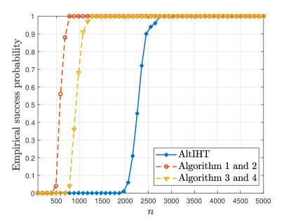
Figure 1: Empirical success rates of three methods under different number of samples.

In Figure 1, the method of Algorithm 1 and 2 benefits from our initialization and requires the least samples. Though the method of Algorithm 3 and 4 also adopts our initialization, it requires more samples because of using the $l_{1}$-norm instead of the nonconvex $l_{0}$-norm. This point also matches the phenomenon that the $l_{0}$-norm would lead to a sharper phase transition curve for linear inverse problems in [35]. The benefit of our initialization could also be verified from the fact that the original AltIHT in [3] requires the most samples.

IV-C Time-data tradeoffs

To verify the time-data tradeoffs phenomenon, we perform Algorithm 1 and our initialization (Algorithm 2) under different numbers of measurements $n_{1}=3000$, $n_{2}=4000$, $n_{3}=5000$. We set $d=m=100$, $s_{\Gamma}^{\star}=400$. The rows of the predictor matrix $\bm{X}$ are generated independently from the distribution $\mathcal{N}(\bm{0},\bm{I}_{d})$. The precision matrix follows a band graph, where $\bm{\Omega}_{ii}^{\star}=1$, $\bm{\Omega}_{i,i+1}^{\star}=\bm{\Omega}_{i+1,i}^{\star}=0.4$ and $\bm{\Omega}_{ij}^{\star}=0$, for ${\lvert}i-j{\rvert}>1$. Each scenario is repeated for 50 trials.

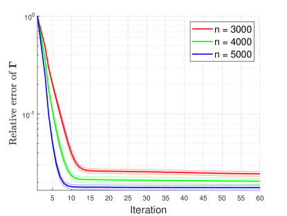
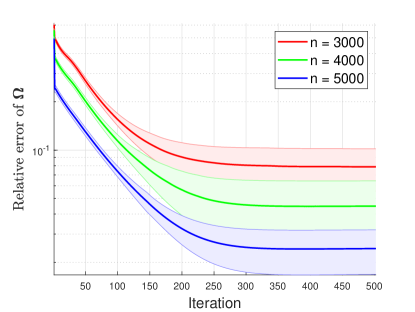
Figure 2: (a) Convergence of ${|\kern-1.125pt|}\bm{\Gamma}_{t}-\bm{\Gamma}_{\star}{|\kern-1.125pt|}_{\mathrm{F}}/{|\kern-1.125pt|}\bm{\Gamma}_{\star}{|\kern-1.125pt|}_{\mathrm{F}}$. (b) Convergence of ${|\kern-1.125pt|}\bm{\Omega}_{t}-\bm{\Omega}_{\star}{|\kern-1.125pt|}_{\mathrm{F}}/{|\kern-1.125pt|}\bm{\Omega}_{\star}{|\kern-1.125pt|}_{\mathrm{F}}$.

In Figure 2 and 2, we present the convergence results for ${|\kern-1.125pt|}\bm{\Gamma}_{t}-\bm{\Gamma}_{\star}{|\kern-1.125pt|}_{\mathrm{F}}/{|\kern-1.125pt|}\bm{\Gamma}_{\star}{|\kern-1.125pt|}_{\mathrm{F}}$ and ${|\kern-1.125pt|}\bm{\Omega}_{t}-\bm{\Omega}_{\star}{|\kern-1.125pt|}_{\mathrm{F}}/{|\kern-1.125pt|}\bm{\Omega}_{\star}{|\kern-1.125pt|}_{\mathrm{F}}$. From the figures we could illustrate more data would lead to faster convergence rates and smaller estimation errors, which support the theoretical result in Theorem 1. For Algorithm 3 and 4 with the $l_{1}$-norm, the results are similar and we do not include them in this manuscript.

IV-D Statistical estimation error

In this part, we verify the scaling of the statistical estimation error of Algorithm 1 and our initialization (Algorithm 2).

We consider two different scenarios, the $\bm{\Gamma}_{\star}$-sparsity dominated case and the $\bm{\Omega}_{\star}$-sparsity dominated case. For the $\bm{\Gamma}_{\star}$-sparsity dominated case, we set $d=m=50$ and consider $s_{\Gamma}^{\star}=200,250,300$ three conditions. For the $\bm{\Omega}_{\star}$-sparsity dominated case, we set $d=50$ and consider $m=56,66,76$ three conditions corresponding to $s_{\Omega}^{\star}=112,132,152$. The rows of the predictor matrix $\bm{X}$ are generated independently from the distribution $\mathcal{N}(\bm{0},\bm{I}_{d})$. The precision matrix follows a block diagonal graph. Every block has the format $(\begin{smallmatrix}1&0.3\\ 0.3&1\end{smallmatrix})$. Each scenario is repeated for 400 trials.

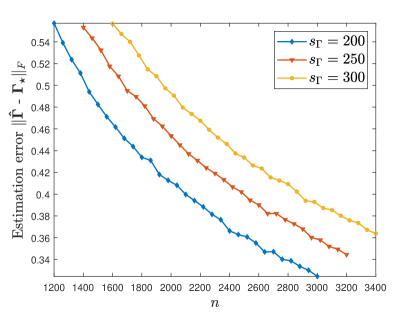
(a) Original numbers of measurements

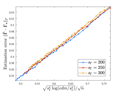
(b) Rescaled numbers of measurements

Figure 3: Estimation error ${|\kern-1.125pt|}\hat{\bm{\Gamma}}-\bm{\Gamma}_{\star}{|\kern-1.125pt|}_{\mathrm{F}}$ under different numbers of measurements $n$ and different sparsity levels.

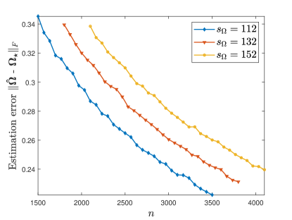
(a) Original numbers of measurements

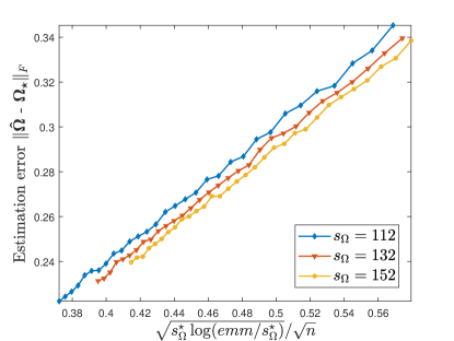
(b) Rescaled numbers of measurements

Figure 4: Estimation error ${|\kern-1.125pt|}\hat{\bm{\Omega}}-\bm{\Omega}_{\star}{|\kern-1.125pt|}_{\mathrm{F}}$ under different numbers of measurements $n$ and different sparsity levels.

The scalings of estimation errors about $\bm{\Gamma}_{\star}$ and $\bm{\Omega}_{\star}$ are presented in Figure 3 and 4. The diagrams illustrate the estimation errors of $\bm{\Gamma}_{\star}$ and $\bm{\Omega}_{\star}$ are proportion to $\omega_{\Gamma}/\sqrt{n}$ and $\omega_{\Omega}/\sqrt{n}$ respectively without any logarithmic factor, which verifies our theoretical result in Theorem 1. For Algorithm 3 and 4 with the $l_{1}$-norm, the results are similar and we do not include them in this manuscript.

IV-E Network structure learning on S&P 500 stock data

In this part, we apply Algorithm 1 and our initialization (Algorithm 2) to analyze the network structure of the stocks in the S&P 500 index. The stock data consists of 1259 daily closing prices for 434 companies in the S&P 500 index between February 8, 2013 and February 7, 2018 [40]. In this way, we get 1259 data vectors, each of which contains the closing prices of all stocks on a trading day. To make the data stationary, we calculate the log-returns $\{\bm{r}_{t}\}_{t=1}^{T-1}$ of stocks by

$$r_{t,i}=\log(\frac{p_{t+1,i}}{p_{t,i}}),\;\;\;t=1,\cdots,T-1,$$ (29)

where $p_{t,i}$ represents the closing price of stock $i$ at day $t$. Then we construct the predictor matrix $\bm{X}=[\bm{r}_{1},\cdots,\bm{r}_{T-2}]^{T}$ and the data matrix $\bm{Y}=[\bm{r}_{2},\cdots,\bm{r}_{T-1}]^{T}$. In the simulation, the step sizes and the constraint parameters are selected through 5-fold cross validation.

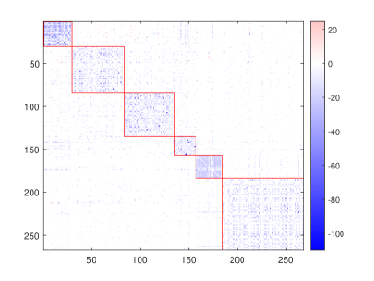
(a) Precision matrix estimated by Algorithm 1 and 2

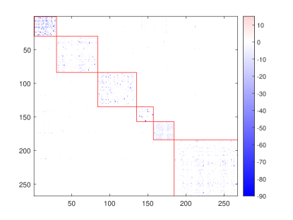
(b) Precision matrix estimated by the method in [3]

Figure 5: Sparsity patterns of precision matrices estimated by two methods. From top left to bottom right, the selected sectors are Energy, Information Technology, Health Care, Materials, Utilities and Financials.

In Figure 5(a), the sparsity pattern of the precision matrix estimated by Algorithm 1 and 2 illustrates that there are strong conditional dependency relationships among the stocks in the same sector. This phenomenon is also recorded in [41]. In Figure 5(b), we also present the sparsity pattern of the precision matrix estimated by the method in [3] for comparison, which indicates similar relationships among the stocks in the same sector.

V Discussion

In this paper, we provide a sharp analysis of a class of alternating projected gradient descent algorithms for the covariate adjusted precision matrix estimation problem. It would be an interesting direction to combine our analysis with practical applications, such as time series models and low rank matrices estimation in [42].

Supplementary for A Sharp Analysis of Covariate Adjusted Precision Matrix Estimation via Alternating Projected Gradient Descent

In this supplementary, we present the complete proof for the theoretical results in the paper. We use $C$ and $c$ to denote positive constants which might change from line to line throughout the paper.

VI Preliminaries

The core of our analysis is the sample-based analysis for the iterations. The following two lemmas illustrate the mixed tails of terms like $\langle\bm{U},\bm{X}^{T}\bm{X}\rangle$ and $\langle\bm{U},\bm{X}^{T}\bm{E}\rangle$, which would appear many times in the remained part.

Lemma 1.

Suppose $\bm{U}\in\mathbb{R}^{d\times d}$, $\bm{X}\in\mathbb{R}^{n\times d}$ and $\text{vec}(\bm{X}^{T})$ follows the distribution $\mathcal{N}(\bm{0},\bm{\Upsilon}_{\bm{X}})$. We have the tail bound

$$P({\lvert}\operatorname{tr}(\bm{X}\bm{U}\bm{X}^{T})-\mathbb{E}\operatorname{tr}(\bm{X}\bm{U}\bm{X}^{T}){\rvert}>u)\leq 2\exp(-c\min(\frac{u^{2}}{n{|\kern-1.125pt|}\bm{\Upsilon}_{\bm{X}}{|\kern-1.125pt|}^{2}{|\kern-1.125pt|}\bm{U}{|\kern-1.125pt|}_{\mathrm{F}}^{2}},\frac{u}{{|\kern-1.125pt|}\bm{\Upsilon}_{\bm{X}}{|\kern-1.125pt|}{|\kern-1.125pt|}\bm{U}{|\kern-1.125pt|}_{\mathrm{F}}})),$$ (30)

where $c$ is a positive constant.

Lemma 2.

Consider $\bm{U}\in\mathbb{R}^{m\times d}$, $\bm{X}\in\mathbb{R}^{n\times d}$ and $\bm{E}\in\mathbb{R}^{n\times m}$. Suppose $\bm{X}$ is independent with $\bm{E}$ and $\text{vec}(\bm{X}^{T})\sim\mathcal{N}(\bm{0},\bm{\Upsilon}_{\bm{X}})$, $\text{vec}(\bm{E}^{T})\sim\mathcal{N}(\bm{0},\bm{\Upsilon}_{\bm{E}})$. Then

$$P({\lvert}\operatorname{tr}(\bm{E}\bm{U}\bm{X}^{T}){\rvert}>u)\leq 2\exp(-c\min(\frac{u^{2}}{n{|\kern-1.125pt|}\bm{\Upsilon}_{\bm{E}}^{\frac{1}{2}}{|\kern-1.125pt|}^{2}{|\kern-1.125pt|}\bm{\Upsilon}_{\bm{X}}^{\frac{1}{2}}{|\kern-1.125pt|}^{2}{|\kern-1.125pt|}\bm{U}{|\kern-1.125pt|}_{\mathrm{F}}^{2}},\frac{u}{{|\kern-1.125pt|}\bm{\Upsilon}_{\bm{E}}^{\frac{1}{2}}{|\kern-1.125pt|}{|\kern-1.125pt|}\bm{\Upsilon}_{\bm{X}}^{\frac{1}{2}}{|\kern-1.125pt|}{|\kern-1.125pt|}\bm{U}{|\kern-1.125pt|}_{\mathrm{F}}})),$$ (31)

where $c$ is a positive constant.

The following lemma is the fundamental tool to analyze the suprema of random processes with a mixed tail, which is based on the generic chaining [39] itself.

Lemma 3.

[43, Theorem 3.5] Let $d_{1}$, $d_{2}$ be two semi-metrics on $T$. Suppose the random process $(X_{t})_{t\in T}$ has a mixed tail

$$P({\lvert}X_{t}-X_{s}{\rvert}>u)\leq 2\exp(-\min(\frac{u^{2}}{d_{2}(t,s)^{2}},\frac{u}{d_{1}(t,s)})),$$ (32)

then we could derive

$$\begin{split}P\big{(}\underset{t\in T}{\sup}\;{\lvert}X_{t}-X_{t_{0}}{\rvert}&>C(\gamma_{2}(T,d_{2})+\gamma_{1}(T,d_{1})+u\Delta_{2}(T)+u^{2}\Delta_{1}(T))\big{)}\leq 2\exp(-u^{2}),\end{split}$$ (33)

where $C$ is a positive constant and $\Delta_{2}(T)$ ($\Delta_{1}(T)$) is the diameter of $T$ with respect to $d_{2}$ ($d_{1}$).

Here, we introduce the definition of $\gamma_{\alpha}$-functional used in the above lemma.

Definition 2 ($\gamma_{\alpha}$-functional).

Let $(T,d)$ be a semi-metric space. For any $0<\alpha<\infty$, the $\gamma_{\alpha}$-functional of $(T,d)$ is defined as

$$\gamma_{\alpha}(T,d)=\underset{\mathcal{T}}{\inf}\;\underset{t\in T}{\sup}\;\sum_{n=0}^{\infty}2^{\frac{n}{\alpha}}d(t,T_{n}),$$ (34)

where $d(t,T_{n})=\underset{s\in T_{n}}{\inf}\;d(t,s)$ and the infimum in (34) is taken over all admissible sequences.

VII Model

The corresponding negative log-likelihood function is

$$\begin{split}f_{n}(\bm{\Gamma},\bm{\Omega})&=-\log{\lvert}\bm{\Omega}{\rvert}+\frac{1}{n}\operatorname{tr}\Big{\{}(\bm{Y}-\bm{X}\bm{\Gamma})\bm{\Omega}(\bm{Y}-\bm{X}\bm{\Gamma})^{T}\Big{\}}\\ &=-\log{\lvert}\bm{\Omega}{\rvert}+\frac{1}{n}\operatorname{tr}\Big{\{}(\bm{\Gamma}-\bm{\Gamma}_{\star})^{T}\bm{X}^{T}\bm{X}(\bm{\Gamma}-\bm{\Gamma}_{\star})\bm{\Omega}-2\bm{E}^{T}\bm{X}(\bm{\Gamma}-\bm{\Gamma}_{\star})\bm{\Omega}+\bm{E}^{T}\bm{E}\bm{\Omega}\Big{\}},\end{split}$$ (35)

where $\bm{X}\in\mathbb{R}^{n\times d}$, $\bm{Y}\in\mathbb{R}^{n\times m}$, $\bm{\Gamma}\in\mathbb{R}^{d\times m}$, $\bm{\Omega}\in\mathbb{R}^{m\times m}$. Without the generality, we suppose $\bm{\Omega}$ is symmetric.

The population loss function is

$$f(\bm{\Gamma},\bm{\Omega})=-\log{\lvert}\bm{\Omega}{\rvert}+\operatorname{tr}\Big{\{}(\bm{\Gamma}-\bm{\Gamma}_{\star})^{T}\bm{\Sigma}_{\bm{X}}(\bm{\Gamma}-\bm{\Gamma}_{\star})\bm{\Omega}+\bm{\Omega}_{\star}^{-1}\bm{\Omega}\Big{\}}.$$ (36)

For the convenience of analysis, we collect the corresponding gradients and Hessian matrices here

$$\nabla_{\Gamma}f_{n}(\bm{\Gamma},\bm{\Omega}) =\frac{2}{n}\bm{X}^{T}\bm{X}(\bm{\Gamma}-\bm{\Gamma}_{\star})\bm{\Omega}-\frac{2}{n}\bm{X}^{T}\bm{E}\bm{\Omega},$$ (37)

$$\nabla_{\Omega}f_{n}(\bm{\Gamma},\bm{\Omega}) =-\bm{\Omega}^{-1}+\frac{1}{n}(\bm{\Gamma}-\bm{\Gamma}_{\star})^{T}\bm{X}^{T}\bm{X}(\bm{\Gamma}-\bm{\Gamma}_{\star})-\frac{2}{n}(\bm{\Gamma}-\bm{\Gamma}_{\star})^{T}\bm{X}^{T}\bm{E}+\frac{1}{n}\bm{E}^{T}\bm{E},$$ (38)

$$\nabla_{\Gamma}f(\bm{\Gamma},\bm{\Omega}) =2\bm{\Sigma}_{\bm{X}}(\bm{\Gamma}-\bm{\Gamma}_{\star})\bm{\Omega},$$ (39)

$$\nabla_{\Omega}f(\bm{\Gamma},\bm{\Omega}) =-\bm{\Omega}^{-1}+(\bm{\Gamma}-\bm{\Gamma}_{\star})^{T}\bm{\Sigma}_{\bm{X}}(\bm{\Gamma}-\bm{\Gamma}_{\star})+\bm{\Omega}_{\star}^{-1},$$ (40)

$$\nabla_{\Gamma}^{2}f(\bm{\Gamma},\bm{\Omega}) =\bm{\Omega}\otimes 2\bm{\Sigma}_{\bm{X}},$$ (41)

$$\nabla_{\Omega}^{2}f(\bm{\Gamma},\bm{\Omega}) =\bm{\Omega}^{-1}\otimes\bm{\Omega}^{-1}.$$ (42)

Here $\nabla_{\Gamma}^{2}f(\bm{\Gamma},\bm{\Omega})$ and $\nabla_{\Omega}^{2}f(\bm{\Gamma},\bm{\Omega})$ is in the sense of vectorization.

In [3], the authors introduce the following local properties of the population function $f(\bm{\Gamma},\bm{\Omega})$ required by the analysis.

Lemma 4.

Under Assumption 1 and 2, for any $\bm{\Gamma},\bm{\Gamma}^{\prime}\in\mathds{B}_{F}(\bm{\Gamma}_{\star};R)$, we have

$$\nu_{\min}\tau_{\min}{|\kern-1.125pt|}\bm{\Gamma}^{\prime}-\bm{\Gamma}{|\kern-1.125pt|}_{\mathrm{F}}^{2}\leq f(\bm{\Gamma}^{\prime},\bm{\Omega}_{\star})-f(\bm{\Gamma},\bm{\Omega}_{\star})-\langle\nabla_{\Gamma}f(\bm{\Gamma},\bm{\Omega}_{\star}),\bm{\Gamma}^{\prime}-\bm{\Gamma}\rangle\leq\nu_{\max}\tau_{\max}{|\kern-1.125pt|}\bm{\Gamma}^{\prime}-\bm{\Gamma}{|\kern-1.125pt|}_{\mathrm{F}}.$$ (43)

Lemma 5.

Under Assumption 1 and 2, for any $\bm{\Omega},\bm{\Omega}^{\prime}\in\mathds{B}_{F}(\bm{\Omega}_{\star};R)$ where $R\leq\frac{\nu_{\min}}{2}$, we have

$$\frac{1}{8\nu_{\max}^{2}}{|\kern-1.125pt|}\bm{\Omega}^{\prime}-\bm{\Omega}{|\kern-1.125pt|}_{\mathrm{F}}^{2}\leq f(\bm{\Gamma}_{\star},\bm{\Omega}^{\prime})-f(\bm{\Gamma}_{\star},\bm{\Omega})-\langle\nabla_{\Omega}f(\bm{\Gamma}_{\star},\bm{\Omega}),\bm{\Omega}^{\prime}-\bm{\Omega}\rangle\leq\frac{2}{\nu_{\min}^{2}}{|\kern-1.125pt|}\bm{\Omega}^{\prime}-\bm{\Omega}{|\kern-1.125pt|}_{\mathrm{F}}.$$ (44)

Lemma 6.

Under Assumption 1 and Assumption 2, for any $\bm{\Omega}\in\mathds{B}_{F}(\bm{\Omega}_{\star};R)$, we could derive

$${|\kern-1.125pt|}\nabla_{\Gamma}f(\bm{\Gamma},\bm{\Omega}_{\star})-\nabla_{\Gamma}f(\bm{\Gamma},\bm{\Omega}){|\kern-1.125pt|}_{\mathrm{F}}\leq 2\tau_{\max}R{|\kern-1.125pt|}\bm{\Omega}-\bm{\Omega}_{\star}{|\kern-1.125pt|}_{\mathrm{F}}.$$ (45)

For any $\bm{\Gamma}\in\mathds{B}_{F}(\bm{\Gamma}_{\star};R)$, we could derive

$${|\kern-1.125pt|}\nabla_{\Omega}f(\bm{\Gamma}_{\star},\bm{\Omega})-\nabla_{\Omega}f(\bm{\Gamma},\bm{\Omega}){|\kern-1.125pt|}_{\mathrm{F}}\leq\tau_{\max}R{|\kern-1.125pt|}\bm{\Gamma}-\bm{\Gamma}_{\star}{|\kern-1.125pt|}_{\mathrm{F}}.$$ (46)

VIII Analysis of the alternating gradient descent with hard thresholding (Proof of Theorem 1)

Our analysis is based on the facts $\bm{\Gamma}_{t}\in\mathds{B}_{F}(\bm{\Gamma}_{\star},R)$ and $\bm{\Omega}_{t}\in\mathds{B}_{F}(\bm{\Omega}_{\star},R)$.

VIII-A Analysis of the iteration about $\bm{\Gamma}$

First, we introduce two helpful lemmas for our analysis.

With the following lemma, we could deal with terms with the hard thresholding operator.

Lemma 7.

[44] Suppose $\bm{x}^{\star}$ is a sparse vector satisfying ${|\kern-1.125pt|}\bm{x}^{\star}{|\kern-1.125pt|}_{0}\leq s_{\star}$. $\mathcal{H}\mathcal{T}(\cdot,s)$ is the hard thresholding operator with $s\geq s_{\star}$. Then we could bound the difference ${|\kern-1.125pt|}\mathcal{H}\mathcal{T}(\bm{x},s)-\bm{x}^{\star}{|\kern-1.125pt|}_{2}$ for any $\bm{x}$ by

$${|\kern-1.125pt|}\mathcal{H}\mathcal{T}(\bm{x},s)-\bm{x}^{\star}{|\kern-1.125pt|}_{2}^{2}\leq(1+\frac{2\sqrt{s_{\star}}}{\sqrt{s-s_{\star}}}){|\kern-1.125pt|}\bm{x}-\bm{x}^{\star}{|\kern-1.125pt|}_{2}^{2}.$$ (47)

The following lemma lays a foundation for the convergence analysis of gradient descent iterations.

Lemma 8.

[45] Suppose $f(\bm{x})$ is $\mu$-strongly convex and $L$-smooth. With the step size $\eta=2/(L+\mu)$, the gradient descent iteration would contract as

$${|\kern-1.125pt|}(\bm{x}-\eta\nabla f(\bm{x})-\bm{x}^{\star}){|\kern-1.125pt|}_{2}\leq\frac{L-\mu}{L+\mu}{|\kern-1.125pt|}\bm{x}-\bm{x}^{\star}{|\kern-1.125pt|}_{2},$$ (48)

where $\bm{x}^{\star}$ is the optimal point.

We set the step sizes as

$$\eta_{\Gamma}=\frac{1}{\nu_{\max}\tau_{\max}+\nu_{\min}\tau_{\min}}\quad\text{and}\quad\eta_{\Omega}=\frac{8\nu_{\max}^{2}\nu_{\min}^{2}}{16\nu_{\max}^{2}+\nu_{\min}^{2}}.$$ (49)

We write $\mathcal{I}=\mathcal{I}_{t+1}\cup\mathcal{I}_{\star}$, where $\mathcal{I}_{t+1}$ and $\mathcal{I}_{\star}$ are the support sets of $\bm{\Gamma}_{t+1}$ and $\bm{\Gamma}_{\star}$, respectively.

Now, we could rewrite ${|\kern-1.125pt|}\bm{\Gamma}_{t+1}-\bm{\Gamma}_{\star}{|\kern-1.125pt|}_{\mathrm{F}}$ as

$${|\kern-1.125pt|}\bm{\Gamma}_{t+1}-\bm{\Gamma}_{\star}{|\kern-1.125pt|}_{\mathrm{F}}$$

$$={|\kern-1.125pt|}\mathcal{H}\mathcal{T}((\bm{\Gamma}_{t}-\eta_{\Gamma}\nabla_{\Gamma}f_{n}(\bm{\Gamma}_{t},\bm{\Omega}_{t}))_{\mathcal{I}},s_{\Gamma})-\bm{\Gamma}_{\star}{|\kern-1.125pt|}_{\mathrm{F}}$$ (50)

$$\leq\sqrt{1+\frac{2\sqrt{s_{\Gamma}^{\star}}}{\sqrt{s_{\Gamma}-s_{\Gamma}^{\star}}}}{|\kern-1.125pt|}(\bm{\Gamma}_{t}-\eta_{\Gamma}\nabla_{\Gamma}f_{n}(\bm{\Gamma}_{t},\bm{\Omega}_{t}))_{\mathcal{I}}-\bm{\Gamma}_{\star}{|\kern-1.125pt|}_{\mathrm{F}}$$ (51)

$$\leq\sqrt{1+\frac{2\sqrt{s_{\Gamma}^{\star}}}{\sqrt{s_{\Gamma}-s_{\Gamma}^{\star}}}}\big{(}{|\kern-1.125pt|}(\bm{\Gamma}_{t}-\eta_{\Gamma}\nabla_{\Gamma}f(\bm{\Gamma}_{t},\bm{\Omega}_{\star}))_{\mathcal{I}}-\bm{\Gamma}_{\star}{|\kern-1.125pt|}_{\mathrm{F}}+\eta_{\Gamma}{|\kern-1.125pt|}(\nabla_{\Gamma}f(\bm{\Gamma}_{t},\bm{\Omega}_{\star})-\nabla_{\Gamma}f_{n}(\bm{\Gamma}_{t},\bm{\Omega}_{t}))_{\mathcal{I}}{|\kern-1.125pt|}_{\mathrm{F}}\big{)}$$

$$\leq\sqrt{1+\frac{2\sqrt{s_{\Gamma}^{\star}}}{\sqrt{s_{\Gamma}-s_{\Gamma}^{\star}}}}\big{(}{|\kern-1.125pt|}\bm{\Gamma}_{t}-\eta_{\Gamma}\nabla_{\Gamma}f(\bm{\Gamma}_{t},\bm{\Omega}_{\star})-\bm{\Gamma}_{\star}{|\kern-1.125pt|}_{\mathrm{F}}+\eta_{\Gamma}{|\kern-1.125pt|}(\nabla_{\Gamma}f(\bm{\Gamma}_{t},\bm{\Omega}_{\star})-\nabla_{\Gamma}f_{n}(\bm{\Gamma}_{t},\bm{\Omega}_{t}))_{\mathcal{I}}{|\kern-1.125pt|}_{\mathrm{F}}\big{)},$$ (52)

where the first inequality is based on Lemma 7.

The first term of (52) could be bounded by the strong convexity and the smoothness of the population function $f(\bm{\Gamma},\bm{\Omega}_{\star})$ about $\bm{\Gamma}$ in Lemma 4 and the corresponding convergence result in Lemma 8

$${|\kern-1.125pt|}\bm{\Gamma}_{t}-\eta_{\Gamma}\nabla_{\Gamma}f(\bm{\Gamma}_{t},\bm{\Omega}_{\star})-\bm{\Gamma}_{\star}{|\kern-1.125pt|}_{\mathrm{F}}\leq\frac{\tau_{\max}\nu_{\max}-\tau_{\min}\nu_{\min}}{\tau_{\max}\nu_{\max}+\tau_{\min}\nu_{\min}}{|\kern-1.125pt|}\bm{\Gamma}_{t}-\bm{\Gamma}_{\star}{|\kern-1.125pt|}_{\mathrm{F}}.$$ (53)

The second term of (52) could be rewritten as

$${|\kern-1.125pt|}(\nabla_{\Gamma}f(\bm{\Gamma}_{t},\bm{\Omega}_{\star})-\nabla_{\Gamma}f_{n}(\bm{\Gamma}_{t},\bm{\Omega}_{t}))_{\mathcal{I}}{|\kern-1.125pt|}_{\mathrm{F}}\leq{|\kern-1.125pt|}\nabla_{\Gamma}f(\bm{\Gamma}_{t},\bm{\Omega}_{\star})-\nabla_{\Gamma}f(\bm{\Gamma}_{t},\bm{\Omega}_{t}){|\kern-1.125pt|}_{\mathrm{F}}+{|\kern-1.125pt|}(\nabla_{\Gamma}f(\bm{\Gamma}_{t},\bm{\Omega}_{t})-\nabla_{\Gamma}f_{n}(\bm{\Gamma}_{t},\bm{\Omega}_{t}))_{\mathcal{I}}{|\kern-1.125pt|}_{\mathrm{F}}.$$ (54)

The first part could be bounded by the Lipschitz property of $\nabla_{\Gamma}f(\bm{\Gamma},\cdot)$ about $\bm{\Omega}$ around $\bm{\Omega}_{\star}$ in Lemma 6

$${|\kern-1.125pt|}\nabla_{\Gamma}f(\bm{\Gamma}_{t},\bm{\Omega}_{\star})-\nabla_{\Gamma}f(\bm{\Gamma}_{t},\bm{\Omega}_{t}){|\kern-1.125pt|}_{\mathrm{F}}\leq 2\tau_{\max}R{|\kern-1.125pt|}\bm{\Omega}_{t}-\bm{\Omega}_{\star}{|\kern-1.125pt|}_{\mathrm{F}}.$$ (55)

The second part is associated with the sample loss function $f_{n}(\bm{\Gamma},\bm{\Omega})$ and needs the sample-based analysis in the following lemma.

Lemma 9.

Under Assumption 1 and 2, we set $\eta_{\Gamma}=\frac{1}{\nu_{\max}\tau_{\max}+\nu_{\min}\tau_{\min}}$. For any $\bm{\Gamma}_{t}\in\mathds{B}_{F}(\bm{\Gamma}_{\star},R)$ and $\bm{\Omega}_{t}\in\mathds{B}_{F}(\bm{\Omega}_{\star},R)$, the difference $(\nabla_{\Gamma}f(\bm{\Gamma}_{t},\bm{\Omega}_{t})-\nabla_{\Gamma}f_{n}(\bm{\Gamma}_{t},\bm{\Omega}_{t}))_{\mathcal{I}}$ could be bounded by

$$\begin{split}&\eta_{\Gamma}{|\kern-1.125pt|}(\nabla_{\Gamma}f(\bm{\Gamma}_{t},\bm{\Omega}_{t})-\nabla_{\Gamma}f_{n}(\bm{\Gamma}_{t},\bm{\Omega}_{t}))_{\mathcal{I}}{|\kern-1.125pt|}_{\mathrm{F}}\\ &\leq C_{\Gamma,1}\frac{\nu_{\max}\tau_{\max}}{\nu_{\max}\tau_{\max}+\nu_{\min}\tau_{\min}}(\frac{R}{\nu_{\max}}\frac{\omega_{\Gamma}+\omega_{\Omega}+u}{\sqrt{n}}{|\kern-1.125pt|}\bm{\Omega}_{t}-\bm{\Omega}_{\star}{|\kern-1.125pt|}_{\mathrm{F}}+\frac{\omega_{\Gamma}+u}{\sqrt{n}}{|\kern-1.125pt|}\bm{\Gamma}_{t}-\bm{\Gamma}_{\star}{|\kern-1.125pt|}_{\mathrm{F}}\\ &+\frac{1}{\sqrt{\tau_{\max}\nu_{\min}}\nu_{\max}}\frac{\omega_{\Gamma}+\omega_{\Omega}+u}{\sqrt{n}}{|\kern-1.125pt|}\bm{\Omega}_{t}-\bm{\Omega}_{\star}{|\kern-1.125pt|}_{\mathrm{F}}+\frac{1}{\sqrt{\tau_{\max}\nu_{\max}}}\frac{\omega_{\Gamma}+u}{\sqrt{n}}),\end{split}$$ (56)

with probability at least $1-8\exp(-u^{2})$, when $n\geq(\omega_{\Gamma}+\omega_{\Omega}+u)^{2}$.

VIII-B Analysis of the iteration about $\bm{\Omega}$

Similarly, we write $\mathcal{T}=\mathcal{T}_{t+1}\cup\mathcal{T}_{\star}$, where $\mathcal{T}_{t+1}$ and $\mathcal{T}_{\star}$ are the support sets of $\bm{\Omega}_{t+1}$ and $\bm{\Omega}_{\star}$, respectively.

For $\mathcal{T}$ contains $\mathcal{T}_{t+1}$ and $\mathcal{T}_{\star}$, we could rearrange ${|\kern-1.125pt|}\bm{\Omega}_{t+1}-\bm{\Omega}_{\star}{|\kern-1.125pt|}_{\mathrm{F}}$ as

$${|\kern-1.125pt|}\bm{\Omega}_{t+1}-\bm{\Omega}_{\star}{|\kern-1.125pt|}_{\mathrm{F}}$$

$$={|\kern-1.125pt|}\mathcal{H}\mathcal{T}((\bm{\Omega}_{t}-\eta_{\Omega}\nabla_{\Omega}f_{n}(\bm{\Gamma}_{t},\bm{\Omega}_{t}))_{\mathcal{T}},s_{\Omega})-\bm{\Omega}_{\star}{|\kern-1.125pt|}_{\mathrm{F}}$$ (57)

$$\leq\sqrt{1+\frac{2\sqrt{s_{\Omega}^{\star}}}{\sqrt{s_{\Omega}-s_{\Omega}^{\star}}}}{|\kern-1.125pt|}(\bm{\Omega}_{t}-\eta_{\Omega}\nabla_{\Omega}f_{n}(\bm{\Gamma}_{t},\bm{\Omega}_{t}))_{\mathcal{T}}-\bm{\Omega}_{\star}{|\kern-1.125pt|}_{\mathrm{F}}$$ (58)

$$\leq\sqrt{1+\frac{2\sqrt{s_{\Omega}^{\star}}}{\sqrt{s_{\Omega}-s_{\Omega}^{\star}}}}\big{(}{|\kern-1.125pt|}(\bm{\Omega}_{t}-\eta_{\Omega}\nabla_{\Omega}f(\bm{\Gamma}_{\star},\bm{\Omega}_{t}))_{\mathcal{T}}-\bm{\Omega}_{\star}{|\kern-1.125pt|}_{\mathrm{F}}+\eta_{\Omega}{|\kern-1.125pt|}(\nabla_{\Omega}f(\bm{\Gamma}_{\star},\bm{\Omega}_{t})-\nabla_{\Omega}f_{n}(\bm{\Gamma}_{t},\bm{\Omega}_{t}))_{\mathcal{T}}{|\kern-1.125pt|}_{\mathrm{F}}\big{)}$$

$$\leq\sqrt{1+\frac{2\sqrt{s_{\Omega}^{\star}}}{\sqrt{s_{\Omega}-s_{\Omega}^{\star}}}}\big{(}{|\kern-1.125pt|}\bm{\Omega}_{t}-\eta_{\Omega}\nabla_{\Omega}f(\bm{\Gamma}_{\star},\bm{\Omega}_{t})-\bm{\Omega}_{\star}{|\kern-1.125pt|}_{\mathrm{F}}+\eta_{\Omega}{|\kern-1.125pt|}(\nabla_{\Omega}f(\bm{\Gamma}_{\star},\bm{\Omega}_{t})-\nabla_{\Omega}f_{n}(\bm{\Gamma}_{t},\bm{\Omega}_{t}))_{\mathcal{T}}{|\kern-1.125pt|}_{\mathrm{F}}\big{)},$$ (59)

where the first inequality is based on Lemma 7.

The first term of (59) could be bounded by the strong convexity and the smoothness of the population function $f(\bm{\Gamma}_{\star},\bm{\Omega})$ about $\bm{\Omega}$ in Lemma 5 and the corresponding convergence result in Lemma 8

$${|\kern-1.125pt|}\bm{\Omega}_{t}-\eta_{\Omega}\nabla_{\Omega}f(\bm{\Gamma}_{\star},\bm{\Omega}_{t})-\bm{\Omega}_{\star}{|\kern-1.125pt|}_{\mathrm{F}}\leq\frac{16\nu_{\max}^{2}-\nu_{\min}^{2}}{16\nu_{\max}^{2}+\nu_{\min}^{2}}{|\kern-1.125pt|}\bm{\Omega}_{t}-\bm{\Omega}_{\star}{|\kern-1.125pt|}_{\mathrm{F}}.$$ (60)

The second term of (59) could be rewritten as

$${|\kern-1.125pt|}(\nabla_{\Omega}f(\bm{\Gamma}_{\star},\bm{\Omega}_{t})-\nabla_{\Omega}f_{n}(\bm{\Gamma}_{t},\bm{\Omega}_{t}))_{\mathcal{T}}{|\kern-1.125pt|}_{\mathrm{F}}\leq{|\kern-1.125pt|}\nabla_{\Omega}f(\bm{\Gamma}_{\star},\bm{\Omega}_{t})-\nabla_{\Omega}f(\bm{\Gamma}_{t},\bm{\Omega}_{t}){|\kern-1.125pt|}_{\mathrm{F}}+{|\kern-1.125pt|}(\nabla_{\Omega}f(\bm{\Gamma}_{t},\bm{\Omega}_{t})-\nabla_{\Omega}f_{n}(\bm{\Gamma}_{t},\bm{\Omega}_{t}))_{\mathcal{T}}{|\kern-1.125pt|}_{\mathrm{F}}.$$ (61)

The first part could be bounded by the Lipschitz property of $\nabla_{\Omega}f(\cdot,\bm{\Omega})$ about $\bm{\Gamma}$ around $\bm{\Gamma}_{\star}$ in Lemma 6

$${|\kern-1.125pt|}\nabla_{\Omega}f(\bm{\Gamma}_{\star},\bm{\Omega}_{t})-\nabla_{\Omega}f(\bm{\Gamma}_{t},\bm{\Omega}_{t}){|\kern-1.125pt|}_{\mathrm{F}}\leq\tau_{\max}R{|\kern-1.125pt|}\bm{\Gamma}_{t}-\bm{\Gamma}_{\star}{|\kern-1.125pt|}_{\mathrm{F}}.$$ (62)

The second part is associated with the sample loss function $f_{n}(\bm{\Gamma},\bm{\Omega})$ and needs the sample-based analysis in the following lemma.

Lemma 10.

Under the same condition as Lemma 9, for any $\bm{\Gamma}_{t}\in\mathds{B}_{F}(\bm{\Gamma}_{\star},R)$ and $\bm{\Omega}_{t}\in\mathds{B}_{F}(\bm{\Omega}_{\star},R)$, the difference $(\nabla_{\Omega}f(\bm{\Gamma}_{t},\bm{\Omega}_{t})-\nabla_{\Omega}f_{n}(\bm{\Gamma}_{t},\bm{\Omega}_{t}))_{\mathcal{T}}$ could be bounded by

$$\begin{split}&\eta_{\Omega}{|\kern-1.125pt|}(\nabla_{\Omega}f(\bm{\Gamma}_{t},\bm{\Omega}_{t})-\nabla_{\Omega}f_{n}(\bm{\Gamma}_{t},\bm{\Omega}_{t}))_{\mathcal{T}}{|\kern-1.125pt|}_{\mathrm{F}}\\ &\leq C_{\Omega,1}\frac{8\nu_{\max}^{2}\nu_{\min}^{2}}{16\nu_{\max}^{2}+\nu_{\min}^{2}}(\tau_{\max}R\frac{\omega_{\Gamma}+\omega_{\Omega}+u}{\sqrt{n}}{|\kern-1.125pt|}\bm{\Gamma}_{t}-\bm{\Gamma}_{\star}{|\kern-1.125pt|}_{\mathrm{F}}+\frac{\sqrt{\tau_{\max}}}{\sqrt{\nu_{\min}}}\frac{\omega_{\Gamma}+\omega_{\Omega}+u}{\sqrt{n}}{|\kern-1.125pt|}\bm{\Gamma}_{t}-\bm{\Gamma}_{\star}{|\kern-1.125pt|}_{\mathrm{F}}+\frac{1}{\nu_{\min}}\frac{\omega_{\Omega}+u}{\sqrt{n}}),\end{split}$$ (63)

with probability at least $1-6\exp(-u^{2})$, when $n\geq(\omega_{\Gamma}+\omega_{\Omega}+u)^{2}$.

VIII-C Analysis of the whole convergence result

We define the convergence parameter $\rho_{\text{pop}}$ associated with the population loss function as

$$\begin{split}\rho_{\text{pop}}&=\max(1-\frac{2\tau_{\min}\nu_{\min}-2\tau_{\max}R}{\tau_{\max}\nu_{\max}+\tau_{\min}\nu_{\min}},1-\frac{2\nu_{\min}^{2}-8\nu_{\max}^{2}\nu_{\min}^{2}\tau_{\max}R}{16\nu_{\max}^{2}+\nu_{\min}^{2}})\\ &\leq\max(1-\frac{\tau_{\min}\nu_{\min}}{\tau_{\max}\nu_{\max}+\tau_{\min}\nu_{\min}},1-\frac{\nu_{\min}^{2}}{16\nu_{\max}^{2}+\nu_{\min}^{2}}),\end{split}$$ (64)

where the inequality is from $R\leq\min(\frac{\tau_{\min}\nu_{\min}}{2\tau_{\max}},\frac{1}{8\tau_{\max}\nu_{\max}^{2}})$, which guarantees $\rho_{\text{pop}}<1$.

By the assumptions $s_{\Gamma}\geq(1+4(1/\rho_{\text{pop}}-1)^{2})s_{\Gamma}^{\star}$ and $s_{\Omega}\geq(1+4(1/\rho_{\text{pop}}-1)^{2})s_{\Omega}^{\star}$, we could bound the two parameters associated with the hard thresholding operation by

$$\max(\sqrt{1+\frac{2\sqrt{s_{\Gamma}^{\star}}}{\sqrt{s_{\Gamma}-s_{\Gamma}^{\star}}}},\sqrt{1+\frac{2\sqrt{s_{\Omega}^{\star}}}{\sqrt{s_{\Omega}-s_{\Omega}^{\star}}}})\leq\frac{1}{\sqrt{\rho_{\text{pop}}}}.$$ (65)

Then, we consider all components of ${|\kern-1.125pt|}\bm{\Gamma}_{t+1}-\bm{\Gamma}_{\star}{|\kern-1.125pt|}_{\mathrm{F}}$. Taking (53), (55) and Lemma 9 into (52), we could derive

$${|\kern-1.125pt|}\bm{\Gamma}_{t+1}-\bm{\Gamma}_{\star}{|\kern-1.125pt|}_{\mathrm{F}}$$

$$\leq\sqrt{1+\frac{2\sqrt{s_{\Gamma}^{\star}}}{\sqrt{s_{\Gamma}-s_{\Gamma}^{\star}}}}\cdot\Big{\{}\frac{\tau_{\max}\nu_{\max}-\tau_{\min}\nu_{\min}}{\tau_{\max}\nu_{\max}+\tau_{\min}\nu_{\min}}{|\kern-1.125pt|}\bm{\Gamma}_{t}-\bm{\Gamma}_{\star}{|\kern-1.125pt|}_{\mathrm{F}}+\frac{2\tau_{\max}R}{\tau_{\max}\nu_{\max}+\tau_{\min}\nu_{\min}}{|\kern-1.125pt|}\bm{\Omega}_{t}-\bm{\Omega}_{\star}{|\kern-1.125pt|}_{\mathrm{F}}$$

$$\qquad+\eta_{\Gamma}\underset{\bm{V}\in\mathcal{C}_{2s_{\Gamma}}\cap\mathcal{S}^{dm-1}}{\sup}\;\langle\bm{V},\nabla_{\Gamma}f(\bm{\Gamma}_{t},\bm{\Omega}_{t})-\nabla_{\Gamma}f_{n}(\bm{\Gamma}_{t},\bm{\Omega}_{t})\rangle\Big{\}}$$

$$\leq(\frac{\rho_{\Gamma,\text{pop}}}{\sqrt{\rho_{\text{pop}}}}+\rho_{\Gamma,\text{sam}})\max({|\kern-1.125pt|}\bm{\Gamma}_{t}-\bm{\Gamma}_{\star}{|\kern-1.125pt|}_{\mathrm{F}},{|\kern-1.125pt|}\bm{\Omega}_{t}-\bm{\Omega}_{\star}{|\kern-1.125pt|}_{\mathrm{F}})+\epsilon_{\Gamma}$$

$$\leq(\sqrt{\rho_{\text{pop}}}+\rho_{\Gamma,\text{sam}})\max({|\kern-1.125pt|}\bm{\Gamma}_{t}-\bm{\Gamma}_{\star}{|\kern-1.125pt|}_{\mathrm{F}},{|\kern-1.125pt|}\bm{\Omega}_{t}-\bm{\Omega}_{\star}{|\kern-1.125pt|}_{\mathrm{F}})+\epsilon_{\Gamma},$$ (66)

where the second inequality is based on the assumption of $s_{\Gamma}$ in (65) and the third inequality is from (64).

Here

$$\rho_{\Gamma,\text{pop}} =\frac{\tau_{\max}\nu_{\max}-\tau_{\min}\nu_{\min}}{\tau_{\max}\nu_{\max}+\tau_{\min}\nu_{\min}}+\frac{2\tau_{\max}R}{\tau_{\max}\nu_{\max}+\tau_{\min}\nu_{\min}}=1-\frac{2\tau_{\min}\nu_{\min}-2\tau_{\max}R}{\tau_{\max}\nu_{\max}+\tau_{\min}\nu_{\min}}$$ (67)

$$\rho_{\Gamma,\text{sam}} =\frac{C_{\Gamma,1}}{\sqrt{\rho_{\text{pop}}}}\frac{\nu_{\max}\tau_{\max}}{\nu_{\max}\tau_{\max}+\nu_{\min}\tau_{\min}}(\frac{R}{\nu_{\max}}\frac{\omega_{\Gamma}+\omega_{\Omega}+u}{\sqrt{n}}+\frac{\omega_{\Gamma}+u}{\sqrt{n}}+\frac{1}{\sqrt{\tau_{\max}\nu_{\min}}\nu_{\max}}\frac{\omega_{\Gamma}+\omega_{\Omega}+u}{\sqrt{n}})$$

$$\leq\frac{C_{\Gamma,2}}{\sqrt{\rho_{\text{pop}}}}\frac{\omega_{\Gamma}+\omega_{\Omega}+u}{\sqrt{n}}$$ (68)

$$\epsilon_{\Gamma} =\frac{C_{\Gamma,1}}{\sqrt{\rho_{\text{pop}}}}\frac{\nu_{\max}\tau_{\max}}{\nu_{\max}\tau_{\max}+\nu_{\min}\tau_{\min}}\frac{1}{\sqrt{\tau_{\max}\nu_{\max}}}\frac{\omega_{\Gamma}+u}{\sqrt{n}}\leq\frac{C_{\Gamma,1}}{\sqrt{\rho_{\text{pop}}}}\frac{1}{\sqrt{\tau_{\max}\nu_{\max}}}\frac{\omega_{\Gamma}+u}{\sqrt{n}}.$$ (69)

If we want ${|\kern-1.125pt|}\bm{\Gamma}_{t+1}-\bm{\Gamma}_{\star}{|\kern-1.125pt|}_{\mathrm{F}}\leq R$, we need to guarantee

$$(\sqrt{\rho_{\text{pop}}}+\rho_{\Gamma,\text{sam}})R+\epsilon_{\Gamma}\leq R$$ (70)

or

$$\epsilon_{\Gamma}+\rho_{\Gamma,\text{sam}}R\leq(1-\sqrt{\rho_{\text{pop}}})R.$$ (71)

Then, we could derive

$$\epsilon_{\Gamma}+\rho_{\Gamma,\text{sam}}R \leq\frac{C_{\Gamma,1}}{\sqrt{\rho_{\text{pop}}}}\frac{\nu_{\max}\tau_{\max}}{\nu_{\max}\tau_{\max}+\nu_{\min}\tau_{\min}}((\frac{R}{\nu_{\max}}\frac{\omega_{\Gamma}+\omega_{\Omega}+u}{\sqrt{n}}+\frac{\omega_{\Gamma}+u}{\sqrt{n}}+\frac{1}{\sqrt{\tau_{\max}\nu_{\min}}\nu_{\max}}\frac{\omega_{\Gamma}+\omega_{\Omega}+u}{\sqrt{n}})R$$

$$\qquad+\frac{1}{\sqrt{\tau_{\max}\nu_{\max}}}\frac{\omega_{\Gamma}+u}{\sqrt{n}})$$

$$\leq\frac{C_{\Gamma,3}}{\sqrt{\rho_{\text{pop}}}}\frac{\omega_{\Gamma}+\omega_{\Omega}+u}{\sqrt{n}}.$$

When the number of measurements satisfies

$$\sqrt{n}\geq C_{\Gamma,3}\frac{\omega_{\Gamma}+\omega_{\Omega}+u}{\sqrt{\rho_{\text{pop}}}(1-\sqrt{\rho_{\text{pop}}})R}$$ (72)

we could guarantee ${|\kern-1.125pt|}\bm{\Gamma}_{t+1}-\bm{\Gamma}_{\star}{|\kern-1.125pt|}_{\mathrm{F}}\leq R$.

Next, we consider all components of ${|\kern-1.125pt|}\bm{\Omega}_{t+1}-\bm{\Omega}_{\star}{|\kern-1.125pt|}_{\mathrm{F}}$. Taking (60), (62) and Lemma 10 into (59), we could derive

$${|\kern-1.125pt|}\bm{\Omega}_{t+1}-\bm{\Omega}_{\star}{|\kern-1.125pt|}_{\mathrm{F}}$$

$$\leq\sqrt{1+\frac{2\sqrt{s_{\Omega}^{\star}}}{\sqrt{s_{\Omega}-s_{\Omega}^{\star}}}}\cdot\Big{\{}\frac{16\nu_{\max}^{2}-\nu_{\min}^{2}}{16\nu_{\max}^{2}+\nu_{\min}^{2}}{|\kern-1.125pt|}\bm{\Omega}_{t}-\bm{\Omega}_{\star}{|\kern-1.125pt|}_{\mathrm{F}}+\frac{8\nu_{\max}^{2}\nu_{\min}^{2}\tau_{\max}R}{16\nu_{\max}^{2}+\nu_{\min}^{2}}{|\kern-1.125pt|}\bm{\Gamma}_{t}-\bm{\Gamma}_{\star}{|\kern-1.125pt|}_{\mathrm{F}}$$

$$\qquad+\eta_{\Omega}\underset{\bm{V}\in\mathcal{C}_{2s_{\Omega}}\cap\mathcal{S}^{m^{2}-1}}{\sup}\;\langle\bm{V},\nabla_{\Omega}f(\bm{\Gamma}_{t},\bm{\Omega}_{t})-\nabla_{\Omega}f_{n}(\bm{\Gamma}_{t},\bm{\Omega}_{t})\rangle\Big{\}}$$

$$\leq(\frac{\rho_{\Omega,\text{pop}}}{\sqrt{\rho_{\text{pop}}}}+\rho_{\Omega,\text{sam}})\max({|\kern-1.125pt|}\bm{\Gamma}_{t}-\bm{\Gamma}_{\star}{|\kern-1.125pt|}_{\mathrm{F}},{|\kern-1.125pt|}\bm{\Omega}_{t}-\bm{\Omega}_{\star}{|\kern-1.125pt|}_{\mathrm{F}})+\epsilon_{\Omega}$$

$$\leq(\sqrt{\rho_{\text{pop}}}+\rho_{\Omega,\text{sam}})\max({|\kern-1.125pt|}\bm{\Gamma}_{t}-\bm{\Gamma}_{\star}{|\kern-1.125pt|}_{\mathrm{F}},{|\kern-1.125pt|}\bm{\Omega}_{t}-\bm{\Omega}_{\star}{|\kern-1.125pt|}_{\mathrm{F}})+\epsilon_{\Omega},$$ (73)

where the second inequality is based on the assumption of $s_{\Omega}$ in (65) and the third inequality is from (64).

Here

$$\rho_{\Omega,\text{pop}} =\frac{16\nu_{\max}^{2}-\nu_{\min}^{2}}{16\nu_{\max}^{2}+\nu_{\min}^{2}}+\frac{8\nu_{\max}^{2}\nu_{\min}^{2}\tau_{\max}R}{16\nu_{\max}^{2}+\nu_{\min}^{2}}=1-\frac{2\nu_{\min}^{2}-8\nu_{\max}^{2}\nu_{\min}^{2}\tau_{\max}R}{16\nu_{\max}^{2}+\nu_{\min}^{2}}$$ (74)

$$\rho_{\Omega,\text{sam}} =\frac{C_{\Omega,1}}{\sqrt{\rho_{\text{pop}}}}\frac{8\nu_{\max}^{2}\nu_{\min}^{2}}{16\nu_{\max}^{2}+\nu_{\min}^{2}}(\tau_{\max}R\frac{\omega_{\Gamma}+\omega_{\Omega}+u}{\sqrt{n}}+\frac{\sqrt{\tau_{\max}}}{\sqrt{\nu_{\min}}}\frac{\omega_{\Gamma}+\omega_{\Omega}+u}{\sqrt{n}})$$

$$\leq\frac{C_{\Omega,2}}{\sqrt{\rho_{\text{pop}}}}\frac{\omega_{\Gamma}+\omega_{\Omega}+u}{\sqrt{n}}$$ (75)

$$\epsilon_{\Omega} =\frac{C_{\Omega,1}}{\sqrt{\rho_{\text{pop}}}}\frac{8\nu_{\max}^{2}\nu_{\min}^{2}}{16\nu_{\max}^{2}+\nu_{\min}^{2}}\frac{1}{\nu_{\min}}\frac{\omega_{\Omega}+u}{\sqrt{n}}\leq\frac{C_{\Omega,1}}{\sqrt{\rho_{\text{pop}}}}\nu_{\min}\frac{\omega_{\Omega}+u}{\sqrt{n}}.$$ (76)

If we want ${|\kern-1.125pt|}\bm{\Omega}_{t+1}-\bm{\Omega}_{\star}{|\kern-1.125pt|}_{\mathrm{F}}\leq R$, we need to guarantee

$$(\sqrt{\rho_{\text{pop}}}+\rho_{\Omega,\text{sam}})R+\epsilon_{\Omega}\leq R$$ (77)

or

$$\epsilon_{\Omega}+\rho_{\Omega,\text{sam}}R\leq(1-\sqrt{\rho_{\text{pop}}})R.$$ (78)

Then, we could derive

$$\epsilon_{\Omega}+\rho_{\Omega,\text{sam}}R \leq\frac{C_{\Omega,1}}{\sqrt{\rho_{\text{pop}}}}\frac{8\nu_{\max}^{2}\nu_{\min}^{2}}{16\nu_{\max}^{2}+\nu_{\min}^{2}}((\tau_{\max}R\frac{\omega_{\Gamma}+\omega_{\Omega}+u}{\sqrt{n}}+\frac{\sqrt{\tau_{\max}}}{\sqrt{\nu_{\min}}}\frac{\omega_{\Gamma}+\omega_{\Omega}+u}{\sqrt{n}})R+\frac{1}{\nu_{\min}}\frac{\omega_{\Omega}+u}{\sqrt{n}})$$

$$\leq\frac{C_{\Omega,3}}{\sqrt{\rho_{\text{pop}}}}\frac{\omega_{\Gamma}+\omega_{\Omega}+u}{\sqrt{n}}.$$

When the number of measurements satisfies

$$\sqrt{n}\geq C_{\Omega,3}\frac{\omega_{\Gamma}+\omega_{\Omega}+u}{\sqrt{\rho_{\text{pop}}}(1-\sqrt{\rho_{\text{pop}}})R},$$ (79)

we could guarantee ${|\kern-1.125pt|}\bm{\Omega}_{t+1}-\bm{\Omega}_{\star}{|\kern-1.125pt|}_{\mathrm{F}}\leq R$.

Finally, we consider ${|\kern-1.125pt|}\bm{\Gamma}_{t+1}-\bm{\Gamma}_{\star}{|\kern-1.125pt|}_{\mathrm{F}}$ and ${|\kern-1.125pt|}\bm{\Omega}_{t+1}-\bm{\Omega}_{\star}{|\kern-1.125pt|}_{\mathrm{F}}$ as a whole and derive

$$\max({|\kern-1.125pt|}\bm{\Gamma}_{t+1}-\bm{\Gamma}_{\star}{|\kern-1.125pt|}_{\mathrm{F}},{|\kern-1.125pt|}\bm{\Omega}_{t+1}-\bm{\Omega}_{\star}{|\kern-1.125pt|}_{\mathrm{F}})$$

$$\leq(\sqrt{\rho_{\text{pop}}}+\max(\rho_{\Gamma,\text{sam}},\rho_{\Omega,\text{sam}}))\max({|\kern-1.125pt|}\bm{\Gamma}_{t}-\bm{\Gamma}_{\star}{|\kern-1.125pt|}_{\mathrm{F}},{|\kern-1.125pt|}\bm{\Omega}_{t}-\bm{\Omega}_{\star}{|\kern-1.125pt|}_{\mathrm{F}})+\max(\epsilon_{\Gamma},\epsilon_{\Omega}).$$ (80)

We also define $\rho_{\text{sam}}=\max(\rho_{\Gamma,\text{sam}},\rho_{\Omega,\text{sam}})$ and $\epsilon=\max(\epsilon_{\Gamma},\epsilon_{\Omega})$.

VIII-D Analysis of initialization (Proof of Theorem 2)

The initialization of $\bm{\Gamma}$ is derived from the following optimization problem

$$\underset{\bm{\Gamma}}{\min}\;\frac{1}{2}{|\kern-1.125pt|}\bm{Y}-\bm{X}\bm{\Gamma}{|\kern-1.125pt|}_{\mathrm{F}}^{2}$$

$$\mathrm{s.t.}\quad{|\kern-1.125pt|}\text{vec}(\bm{\Gamma}^{T}){|\kern-1.125pt|}_{0}\leq s_{\Gamma}.$$ (81)

The initialization of $\bm{\Omega}$ is derived from the following optimization problem

$$\underset{\bm{\Omega}}{\min}\;\frac{1}{2}{|\kern-1.125pt|}\bm{\Omega}-\bm{S}^{-1}{|\kern-1.125pt|}_{\mathrm{F}}^{2}$$

$$\mathrm{s.t.}\quad{|\kern-1.125pt|}\text{vec}(\bm{\Omega}^{T}){|\kern-1.125pt|}_{0}\leq s_{\Omega},$$ (82)

where $\bm{S}=(\bm{Y}-\bm{X}\bm{\Gamma}_{\text{ini}})^{T}(\bm{Y}-\bm{X}\bm{\Gamma}_{\text{ini}})/n$.

The error ${|\kern-1.125pt|}\bm{\Gamma}_{\text{ini}}-\bm{\Gamma}_{\star}{|\kern-1.125pt|}_{\mathrm{F}}$ is analyzed as the Lasso.

Lemma 11.

When $\sqrt{n}\geq C_{\Gamma,4}\frac{\tau_{\max}}{\tau_{\min}}(\omega_{\Gamma}+u)$, we could derive

$${|\kern-1.125pt|}\bm{\Gamma}_{\text{ini}}-\bm{\Gamma}_{\star}{|\kern-1.125pt|}_{\mathrm{F}}\leq C_{\Gamma,5}\frac{\omega_{\Gamma}+u}{\sqrt{n}}\frac{\tau_{\max}^{\frac{1}{2}}}{\tau_{\min}\nu_{\min}^{\frac{1}{2}}},$$ (83)

with probability at least $1-4\exp(-u^{2})$.

When $n\geq C_{\Gamma,6}(\omega_{\Gamma}+u)^{2}/R^{2}$, we could derive

$${|\kern-1.125pt|}\bm{\Gamma}_{\text{ini}}-\bm{\Gamma}_{\star}{|\kern-1.125pt|}_{\mathrm{F}}\leq R.$$ (84)

The analysis of ${|\kern-1.125pt|}\bm{\Omega}_{\text{ini}}-\bm{\Omega}_{\star}{|\kern-1.125pt|}_{\mathrm{F}}$ is more complicated.

Lemma 12.

When $\sqrt{n}>C_{\Omega,4}\frac{\tau_{\max}\nu_{\max}}{\tau_{\min}\nu_{\min}}(m+\omega_{\Gamma}+u)$, we could derive

$${|\kern-1.125pt|}\bm{\Omega}_{\text{ini}}-\bm{\Omega}_{\star}{|\kern-1.125pt|}_{\mathrm{F}}\leq C_{\Omega,5}\frac{\tau_{\max}^{2}\nu_{\max}^{2}}{\tau_{\min}^{2}\nu_{\min}}\frac{m+\omega_{\Gamma}+u}{\sqrt{n}},$$ (85)

with probability at least $1-18\exp(-u^{2})$.

When $n>C_{\Omega,6}(m+\omega_{\Gamma}+u)^{2}/R^{2}$, we could derive ${|\kern-1.125pt|}\bm{\Omega}_{\text{ini}}-\bm{\Omega}_{\star}{|\kern-1.125pt|}_{\mathrm{F}}\leq R$.

IX Analysis of alternating projected gradient descent for general convex regularizers (Proof of Theorem 3)

Our analysis is based on the facts $\bm{\Gamma}_{t}\in\mathds{B}_{F}(\bm{\Gamma}_{\star},R)$ and $\bm{\Omega}_{t}\in\mathds{B}_{F}(\bm{\Omega}_{\star},R)$.

IX-A Analysis of the iteration about $\bm{\Gamma}$

With the following lemma, we could bound the distance between the point after projection and the point in the constraint by a supremum of a series of inner products.

Lemma 13.

Suppose $\bar{\bm{x}}=\mathcal{P}_{\mathcal{K}}(\bm{y})$, where $\mathcal{K}=\{\bm{x}\mid\mathcal{R}(\bm{x})\leq\mathcal{R}(\bm{x}^{\star})\}$ and $\mathcal{R}(\cdot)$ is a convex function. Then we could bound ${|\kern-1.125pt|}\bar{\bm{x}}-\bm{x}^{\star}{|\kern-1.125pt|}_{2}$ as

$${|\kern-1.125pt|}\bar{\bm{x}}-\bm{x}^{\star}{|\kern-1.125pt|}_{2}\leq\underset{\bm{v}\in\mathcal{C}\cap\SS_{2}}{\sup}\;\langle\bm{v},\bm{y}-\bm{x}^{\star}\rangle,$$ (86)

where $\mathcal{C}=\mathrm{cone}(\mathcal{D})$ is the decent cone, $\mathcal{D}=\mathcal{K}-\{\bm{x}^{\star}\}$ is the descent set and $\SS_{2}$ is the sphere with unit Euclidean norm.

Now, we could rewrite ${|\kern-1.125pt|}\bm{\Gamma}_{t+1}-\bm{\Gamma}_{\star}{|\kern-1.125pt|}_{\mathrm{F}}$ as

$${|\kern-1.125pt|}\bm{\Gamma}_{t+1}-\bm{\Gamma}_{\star}{|\kern-1.125pt|}_{\mathrm{F}}$$

$$={|\kern-1.125pt|}\mathcal{P}_{\mathcal{K}_{\Gamma}}(\bm{\Gamma}_{t}-\eta_{\Gamma}\nabla_{\Gamma}f_{n}(\bm{\Gamma}_{t},\bm{\Omega}_{t}))-\bm{\Gamma}_{\star}{|\kern-1.125pt|}_{\mathrm{F}}$$ (87)

$$\leq\underset{\bm{V}\in\mathcal{C}_{\Gamma}\cap\mathcal{S}^{dm-1}}{\sup}\;\langle\bm{V},\bm{\Gamma}_{t}-\bm{\Gamma}_{\star}-\eta_{\Gamma}\nabla_{\Gamma}f_{n}(\bm{\Gamma}_{t},\bm{\Omega}_{t})\rangle$$ (88)

$$=\underset{\bm{V}\in\mathcal{C}_{\Gamma}\cap\mathcal{S}^{dm-1}}{\sup}\;\langle\bm{V},\bm{\Gamma}_{t}-\bm{\Gamma}_{\star}-\eta_{\Gamma}\nabla_{\Gamma}f(\bm{\Gamma}_{t},\bm{\Omega}_{\star})$$ (89)

$$\qquad+\eta_{\Gamma}(\nabla_{\Gamma}f(\bm{\Gamma}_{t},\bm{\Omega}_{\star})-\nabla_{\Gamma}f(\bm{\Gamma}_{t},\bm{\Omega}_{t}))+\eta_{\Gamma}(\nabla_{\Gamma}f(\bm{\Gamma}_{t},\bm{\Omega}_{t})-\nabla_{\Gamma}f_{n}(\bm{\Gamma}_{t},\bm{\Omega}_{t}))\rangle$$ (90)

$$\leq{|\kern-1.125pt|}\bm{\Gamma}_{t}-\eta_{\Gamma}\nabla_{\Gamma}f(\bm{\Gamma}_{t},\bm{\Omega}_{\star})-\bm{\Gamma}_{\star}{|\kern-1.125pt|}_{\mathrm{F}}+\eta_{\Gamma}{|\kern-1.125pt|}\nabla_{\Gamma}f(\bm{\Gamma}_{t},\bm{\Omega}_{\star})-\nabla_{\Gamma}f(\bm{\Gamma}_{t},\bm{\Omega}_{t}){|\kern-1.125pt|}_{\mathrm{F}}$$ (91)

$$\qquad+\eta_{\Gamma}\underset{\bm{V}\in\mathcal{C}_{\Gamma}\cap\mathcal{S}^{dm-1}}{\sup}\;\langle\bm{V},\nabla_{\Gamma}f(\bm{\Gamma}_{t},\bm{\Omega}_{t})-\nabla_{\Gamma}f_{n}(\bm{\Gamma}_{t},\bm{\Omega}_{t})\rangle,$$ (92)

where the first inequality is based on Lemma 13 and the last inequality is from the Cauchy–Schwarz inequality.

The first and second terms of (92) have been bounded in the previous analysis.

The third term of (92) could be analyzed in the same way as Lemma 9 with a different set $\mathcal{C}_{\Gamma}$.

Lemma 14.

Under Assumption 1 and 2, we set $\eta_{\Gamma}=\frac{1}{\nu_{\max}\tau_{\max}+\nu_{\min}\tau_{\min}}$. For any $\bm{\Gamma}_{t}\in\mathds{B}_{F}(\bm{\Gamma}_{\star},R)$ and $\bm{\Omega}_{t}\in\mathds{B}_{F}(\bm{\Omega}_{\star},R)$, the term $\eta_{\Gamma}\underset{\bm{V}\in\mathcal{C}_{\Gamma}\cap\mathcal{S}^{dm-1}}{\sup}\;\langle\bm{V},\nabla_{\Gamma}f(\bm{\Gamma}_{t},\bm{\Omega}_{t})-\nabla_{\Gamma}f_{n}(\bm{\Gamma}_{t},\bm{\Omega}_{t})\rangle$ could be bounded by

$$\begin{split}&\eta_{\Gamma}\underset{\bm{V}\in\mathcal{C}_{\Gamma}\cap\mathcal{S}^{dm-1}}{\sup}\;\langle\bm{V},\nabla_{\Gamma}f(\bm{\Gamma}_{t},\bm{\Omega}_{t})-\nabla_{\Gamma}f_{n}(\bm{\Gamma}_{t},\bm{\Omega}_{t})\rangle\\ &\leq C_{\Gamma,1}\frac{\nu_{\max}\tau_{\max}}{\nu_{\max}\tau_{\max}+\nu_{\min}\tau_{\min}}(\frac{R}{\nu_{\max}}\frac{\bar{\omega}_{\Gamma}+\bar{\omega}_{\Omega}+u}{\sqrt{n}}{|\kern-1.125pt|}\bm{\Omega}_{t}-\bm{\Omega}_{\star}{|\kern-1.125pt|}_{\mathrm{F}}+\frac{\bar{\omega}_{\Gamma}+u}{\sqrt{n}}{|\kern-1.125pt|}\bm{\Gamma}_{t}-\bm{\Gamma}_{\star}{|\kern-1.125pt|}_{\mathrm{F}}\\ &+\frac{1}{\sqrt{\tau_{\max}\nu_{\min}}\nu_{\max}}\frac{\bar{\omega}_{\Gamma}+\bar{\omega}_{\Omega}+u}{\sqrt{n}}{|\kern-1.125pt|}\bm{\Omega}_{t}-\bm{\Omega}_{\star}{|\kern-1.125pt|}_{\mathrm{F}}+\frac{1}{\sqrt{\tau_{\max}\nu_{\max}}}\frac{\bar{\omega}_{\Gamma}+u}{\sqrt{n}}),\end{split}$$ (93)

with probability at least $1-8\exp(-u^{2})$, when $n\geq(\bar{\omega}_{\Gamma}+\bar{\omega}_{\Omega}+u)^{2}$.

IX-B Analysis of the iteration about $\bm{\Omega}$

First, we could rearrange ${|\kern-1.125pt|}\bm{\Omega}_{t+1}-\bm{\Omega}_{\star}{|\kern-1.125pt|}_{\mathrm{F}}$ as

$${|\kern-1.125pt|}\bm{\Omega}_{t+1}-\bm{\Omega}_{\star}{|\kern-1.125pt|}_{\mathrm{F}}$$

$$={|\kern-1.125pt|}\mathcal{P}_{\mathcal{K}_{\Omega}}(\bm{\Omega}_{t}-\eta_{\Omega}\nabla_{\Omega}f_{n}(\bm{\Gamma}_{t},\bm{\Omega}_{t}))-\bm{\Omega}_{\star}{|\kern-1.125pt|}_{\mathrm{F}}$$ (94)

$$\leq\underset{\bm{V}\in\mathcal{C}_{\Omega}\cap\mathcal{S}^{m^{2}-1}}{\sup}\;\langle\bm{V},\bm{\Omega}_{t}-\bm{\Omega}_{\star}-\eta_{\Omega}\nabla_{\Omega}f_{n}(\bm{\Gamma}_{t},\bm{\Omega}_{t})\rangle$$ (95)

$$=\underset{\bm{V}\in\mathcal{C}_{\Omega}\cap\mathcal{S}^{m^{2}-1}}{\sup}\;\langle\bm{V},\bm{\Omega}_{t}-\bm{\Omega}_{\star}-\eta_{\Omega}\nabla_{\Omega}f(\bm{\Gamma}_{\star},\bm{\Omega}_{t})$$ (96)

$$\qquad+\eta_{\Omega}(\nabla_{\Omega}f(\bm{\Gamma}_{\star},\bm{\Omega}_{t})-\nabla_{\Omega}f(\bm{\Gamma}_{t},\bm{\Omega}_{t}))+\eta_{\Omega}(\nabla_{\Omega}f(\bm{\Gamma}_{t},\bm{\Omega}_{t})-\nabla_{\Omega}f_{n}(\bm{\Gamma}_{t},\bm{\Omega}_{t}))\rangle$$ (97)

$$\leq{|\kern-1.125pt|}\bm{\Omega}_{t}-\eta_{\Omega}\nabla_{\Omega}f(\bm{\Gamma}_{\star},\bm{\Omega}_{t})-\bm{\Omega}_{\star}{|\kern-1.125pt|}_{\mathrm{F}}+\eta_{\Omega}{|\kern-1.125pt|}\nabla_{\Omega}f(\bm{\Gamma}_{\star},\bm{\Omega}_{t})-\nabla_{\Omega}f(\bm{\Gamma}_{t},\bm{\Omega}_{t}){|\kern-1.125pt|}_{\mathrm{F}}$$ (98)

$$\qquad+\eta_{\Omega}\underset{\bm{V}\in\mathcal{C}_{\Omega}\cap\mathcal{S}^{m^{2}-1}}{\sup}\;\langle\bm{V},\nabla_{\Omega}f(\bm{\Gamma}_{t},\bm{\Omega}_{t})-\nabla_{\Omega}f_{n}(\bm{\Gamma}_{t},\bm{\Omega}_{t})\rangle,$$ (99)

where the first inequality is based on Lemma 13 and the last inequality is from the Cauchy–Schwarz inequality.

The first and second terms of (99) have been bounded in the previous analysis.

The third term of (99) could be analyzed in the same way as Lemma 10 with a different set $\mathcal{C}_{\Omega}$.

Lemma 15.

Under the same condition as Lemma 14. For any $\bm{\Gamma}_{t}\in\mathds{B}_{F}(\bm{\Gamma}_{\star},R)$ and $\bm{\Omega}_{t}\in\mathds{B}_{F}(\bm{\Omega}_{\star},R)$, the term
$\eta_{\Omega}\underset{\bm{V}\in\mathcal{C}_{\Omega}\cap\mathcal{S}^{m^{2}-1}}{\sup}\;\langle\bm{V},\nabla_{\Omega}f(\bm{\Gamma}_{t},\bm{\Omega}_{t})-\nabla_{\Omega}f_{n}(\bm{\Gamma}_{t},\bm{\Omega}_{t})\rangle$ could be bounded by

$$\begin{split}&\eta_{\Omega}\underset{\bm{V}\in\mathcal{C}_{\Omega}\cap\mathcal{S}^{m^{2}-1}}{\sup}\;\langle\bm{V},\nabla_{\Omega}f(\bm{\Gamma}_{t},\bm{\Omega}_{t})-\nabla_{\Omega}f_{n}(\bm{\Gamma}_{t},\bm{\Omega}_{t})\rangle\\ &\leq C_{\Omega,1}\frac{8\nu_{\max}^{2}\nu_{\min}^{2}}{16\nu_{\max}^{2}+\nu_{\min}^{2}}(\tau_{\max}R\frac{\bar{\omega}_{\Gamma}+\bar{\omega}_{\Omega}+u}{\sqrt{n}}{|\kern-1.125pt|}\bm{\Gamma}_{t}-\bm{\Gamma}_{\star}{|\kern-1.125pt|}_{\mathrm{F}}+\frac{\sqrt{\tau_{\max}}}{\sqrt{\nu_{\min}}}\frac{\bar{\omega}_{\Gamma}+\bar{\omega}_{\Omega}+u}{\sqrt{n}}{|\kern-1.125pt|}\bm{\Gamma}_{t}-\bm{\Gamma}_{\star}{|\kern-1.125pt|}_{\mathrm{F}}+\frac{1}{\nu_{\min}}\frac{\bar{\omega}_{\Omega}+u}{\sqrt{n}}),\end{split}$$ (100)

with probability at least $1-6\exp(-u^{2})$, when $n\geq(\bar{\omega}_{\Gamma}+\bar{\omega}_{\Omega}+u)^{2}$.

IX-C Analysis of the whole convergence result

Then, we consider all components of ${|\kern-1.125pt|}\bm{\Gamma}_{t+1}-\bm{\Gamma}_{\star}{|\kern-1.125pt|}_{\mathrm{F}}$ and derive

$${|\kern-1.125pt|}\bm{\Gamma}_{t+1}-\bm{\Gamma}_{\star}{|\kern-1.125pt|}_{\mathrm{F}}$$

$$\leq\frac{\tau_{\max}\nu_{\max}-\tau_{\min}\nu_{\min}}{\tau_{\max}\nu_{\max}+\tau_{\min}\nu_{\min}}{|\kern-1.125pt|}\bm{\Gamma}_{t}-\bm{\Gamma}_{\star}{|\kern-1.125pt|}_{\mathrm{F}}+\frac{2\tau_{\max}R}{\tau_{\max}\nu_{\max}+\tau_{\min}\nu_{\min}}{|\kern-1.125pt|}\bm{\Omega}_{t}-\bm{\Omega}_{\star}{|\kern-1.125pt|}_{\mathrm{F}}$$

$$\qquad+\eta_{\Gamma}\underset{\bm{V}\in\mathcal{C}_{\Gamma}\cap\mathcal{S}^{dm-1}}{\sup}\;\langle\bm{V},\nabla_{\Gamma}f(\bm{\Gamma}_{t},\bm{\Omega}_{t})-\nabla_{\Gamma}f_{n}(\bm{\Gamma}_{t},\bm{\Omega}_{t})\rangle$$

$$\leq(\rho_{\Gamma,\text{pop}}+\rho_{\Gamma,\text{sam}})\max({|\kern-1.125pt|}\bm{\Gamma}_{t}-\bm{\Gamma}_{\star}{|\kern-1.125pt|}_{\mathrm{F}},{|\kern-1.125pt|}\bm{\Omega}_{t}-\bm{\Omega}_{\star}{|\kern-1.125pt|}_{\mathrm{F}})+\epsilon_{\Gamma},$$ (101)

where

$$\rho_{\Gamma,\text{pop}} =\frac{\tau_{\max}\nu_{\max}-\tau_{\min}\nu_{\min}}{\tau_{\max}\nu_{\max}+\tau_{\min}\nu_{\min}}+\frac{2\tau_{\max}R}{\tau_{\max}\nu_{\max}+\tau_{\min}\nu_{\min}}=1-\frac{2\tau_{\min}\nu_{\min}-2\tau_{\max}R}{\tau_{\max}\nu_{\max}+\tau_{\min}\nu_{\min}}$$ (102)

$$\rho_{\Gamma,\text{sam}} =C_{\Gamma,1}\frac{\nu_{\max}\tau_{\max}}{\nu_{\max}\tau_{\max}+\nu_{\min}\tau_{\min}}(\frac{R}{\nu_{\max}}\frac{\bar{\omega}_{\Gamma}+\bar{\omega}_{\Omega}+u}{\sqrt{n}}+\frac{\bar{\omega}_{\Gamma}+u}{\sqrt{n}}+\frac{1}{\sqrt{\tau_{\max}\nu_{\min}}\nu_{\max}}\frac{\bar{\omega}_{\Gamma}+\bar{\omega}_{\Omega}+u}{\sqrt{n}})$$

$$\leq C_{\Gamma,2}\frac{\bar{\omega}_{\Gamma}+\bar{\omega}_{\Omega}+u}{\sqrt{n}}$$ (103)

$$\epsilon_{\Gamma} =C_{\Gamma,1}\frac{\nu_{\max}\tau_{\max}}{\nu_{\max}\tau_{\max}+\nu_{\min}\tau_{\min}}\frac{1}{\sqrt{\tau_{\max}\nu_{\max}}}\frac{\bar{\omega}_{\Gamma}+u}{\sqrt{n}}\leq C_{\Gamma,1}\frac{1}{\sqrt{\tau_{\max}\nu_{\max}}}\frac{\bar{\omega}_{\Gamma}+u}{\sqrt{n}}.$$ (104)

If we want ${|\kern-1.125pt|}\bm{\Gamma}_{t+1}-\bm{\Gamma}_{\star}{|\kern-1.125pt|}_{\mathrm{F}}\leq R$, we need to guarantee

$$(\rho_{\Gamma,\text{pop}}+\rho_{\Gamma,\text{sam}})R+\epsilon_{\Gamma}\leq R$$ (105)

or

$$\epsilon_{\Gamma}+\rho_{\Gamma,\text{sam}}R\leq(1-\rho_{\text{pop}})R.$$ (106)

Then, we could derive

$$\epsilon_{\Gamma}+\rho_{\Gamma,\text{sam}}R \leq C_{\Gamma,1}\frac{\nu_{\max}\tau_{\max}}{\nu_{\max}\tau_{\max}+\nu_{\min}\tau_{\min}}((\frac{R}{\nu_{\max}}\frac{\bar{\omega}_{\Gamma}+\bar{\omega}_{\Omega}+u}{\sqrt{n}}+\frac{\bar{\omega}_{\Gamma}+u}{\sqrt{n}}+\frac{1}{\sqrt{\tau_{\max}\nu_{\min}}\nu_{\max}}\frac{\bar{\omega}_{\Gamma}+\bar{\omega}_{\Omega}+u}{\sqrt{n}})R$$

$$\qquad+\frac{1}{\sqrt{\tau_{\max}\nu_{\max}}}\frac{\bar{\omega}_{\Gamma}+u}{\sqrt{n}})$$

$$\leq C_{\Gamma,3}\frac{\bar{\omega}_{\Gamma}+\bar{\omega}_{\Omega}+u}{\sqrt{n}}.$$

When the number of measurements satisfies

$$\sqrt{n}\geq C_{\Gamma,3}\frac{\bar{\omega}_{\Gamma}+\bar{\omega}_{\Omega}+u}{(1-\rho_{\Gamma,\text{pop}})R}$$ (107)

we could guarantee ${|\kern-1.125pt|}\bm{\Gamma}_{t+1}-\bm{\Gamma}_{\star}{|\kern-1.125pt|}_{\mathrm{F}}\leq R$.

Next, we consider all components of ${|\kern-1.125pt|}\bm{\Omega}_{t+1}-\bm{\Omega}_{\star}{|\kern-1.125pt|}_{\mathrm{F}}$ and derive

$${|\kern-1.125pt|}\bm{\Omega}_{t+1}-\bm{\Omega}_{\star}{|\kern-1.125pt|}_{\mathrm{F}}$$

$$\leq\frac{16\nu_{\max}^{2}-\nu_{\min}^{2}}{16\nu_{\max}^{2}+\nu_{\min}^{2}}{|\kern-1.125pt|}\bm{\Omega}_{t}-\bm{\Omega}_{\star}{|\kern-1.125pt|}_{\mathrm{F}}+\frac{8\nu_{\max}^{2}\nu_{\min}^{2}\tau_{\max}R}{16\nu_{\max}^{2}+\nu_{\min}^{2}}{|\kern-1.125pt|}\bm{\Gamma}_{t}-\bm{\Gamma}_{\star}{|\kern-1.125pt|}_{\mathrm{F}}$$

$$\qquad+\eta_{\Omega}\underset{\bm{V}\in\mathcal{C}_{\Omega}\cap\mathcal{S}^{m^{2}-1}}{\sup}\;\langle\bm{V},\nabla_{\Omega}f(\bm{\Gamma}_{t},\bm{\Omega}_{t})-\nabla_{\Omega}f_{n}(\bm{\Gamma}_{t},\bm{\Omega}_{t})\rangle$$

$$\leq(\rho_{\Omega,\text{pop}}+\rho_{\Omega,\text{sam}})\max({|\kern-1.125pt|}\bm{\Gamma}_{t}-\bm{\Gamma}_{\star}{|\kern-1.125pt|}_{\mathrm{F}},{|\kern-1.125pt|}\bm{\Omega}_{t}-\bm{\Omega}_{\star}{|\kern-1.125pt|}_{\mathrm{F}})+\epsilon_{\Omega},$$ (108)

where

$$\rho_{\Omega,\text{pop}} =\frac{16\nu_{\max}^{2}-\nu_{\min}^{2}}{16\nu_{\max}^{2}+\nu_{\min}^{2}}+\frac{8\nu_{\max}^{2}\nu_{\min}^{2}\tau_{\max}R}{16\nu_{\max}^{2}+\nu_{\min}^{2}}=1-\frac{2\nu_{\min}^{2}-8\nu_{\max}^{2}\nu_{\min}^{2}\tau_{\max}R}{16\nu_{\max}^{2}+\nu_{\min}^{2}}$$ (109)

$$\rho_{\Omega,\text{sam}} =C_{\Omega,1}\frac{8\nu_{\max}^{2}\nu_{\min}^{2}}{16\nu_{\max}^{2}+\nu_{\min}^{2}}(\tau_{\max}R\frac{\bar{\omega}_{\Gamma}+\bar{\omega}_{\Omega}+u}{\sqrt{n}}+\frac{\sqrt{\tau_{\max}}}{\sqrt{\nu_{\min}}}\frac{\bar{\omega}_{\Gamma}+\bar{\omega}_{\Omega}+u}{\sqrt{n}})$$

$$\leq C_{\Omega,2}\frac{\bar{\omega}_{\Gamma}+\bar{\omega}_{\Omega}+u}{\sqrt{n}}$$ (110)

$$\epsilon_{\Omega} =C_{\Omega,1}\frac{8\nu_{\max}^{2}\nu_{\min}^{2}}{16\nu_{\max}^{2}+\nu_{\min}^{2}}\frac{1}{\nu_{\min}}\frac{\bar{\omega}_{\Omega}+u}{\sqrt{n}}\leq C_{\Omega,1}\nu_{\min}\frac{\bar{\omega}_{\Omega}+u}{\sqrt{n}}.$$ (111)

If we want ${|\kern-1.125pt|}\bm{\Omega}_{t+1}-\bm{\Omega}_{\star}{|\kern-1.125pt|}_{\mathrm{F}}\leq R$, we need to guarantee

$$(\rho_{\Omega,\text{pop}}+\rho_{\Omega,\text{sam}})R+\epsilon_{\Omega}\leq R$$ (112)

or

$$\epsilon_{\Omega}+\rho_{\Omega,\text{sam}}R\leq(1-\rho_{\Omega,\text{pop}})R.$$ (113)

Then, we could derive

$$\epsilon_{\Omega}+\rho_{\Omega,\text{sam}}R \leq C_{\Omega,1}\frac{8\nu_{\max}^{2}\nu_{\min}^{2}}{16\nu_{\max}^{2}+\nu_{\min}^{2}}((\tau_{\max}R\frac{\bar{\omega}_{\Gamma}+\bar{\omega}_{\Omega}+u}{\sqrt{n}}+\frac{\sqrt{\tau_{\max}}}{\sqrt{\nu_{\min}}}\frac{\bar{\omega}_{\Gamma}+\bar{\omega}_{\Omega}+u}{\sqrt{n}})R+\frac{1}{\nu_{\min}}\frac{\bar{\omega}_{\Omega}+u}{\sqrt{n}})$$

$$\leq C_{\Omega,3}\frac{\bar{\omega}_{\Gamma}+\bar{\omega}_{\Omega}+u}{\sqrt{n}}.$$

When the number of measurements satisfies

$$\sqrt{n}\geq C_{\Omega,3}\frac{\bar{\omega}_{\Gamma}+\bar{\omega}_{\Omega}+u}{(1-\rho_{\Omega,\text{pop}})R},$$ (114)

we could guarantee ${|\kern-1.125pt|}\bm{\Omega}_{t+1}-\bm{\Omega}_{\star}{|\kern-1.125pt|}_{\mathrm{F}}\leq R$.

Finally, we consider ${|\kern-1.125pt|}\bm{\Gamma}_{t+1}-\bm{\Gamma}_{\star}{|\kern-1.125pt|}_{\mathrm{F}}$ and ${|\kern-1.125pt|}\bm{\Omega}_{t+1}-\bm{\Omega}_{\star}{|\kern-1.125pt|}_{\mathrm{F}}$ as a whole and derive

$$\max({|\kern-1.125pt|}\bm{\Gamma}_{t+1}-\bm{\Gamma}_{\star}{|\kern-1.125pt|}_{\mathrm{F}},{|\kern-1.125pt|}\bm{\Omega}_{t+1}-\bm{\Omega}_{\star}{|\kern-1.125pt|}_{\mathrm{F}})$$

$$\leq(\max(\rho_{\Gamma,\text{pop}},\rho_{\Omega,\text{pop}})+\max(\rho_{\Gamma,\text{sam}},\rho_{\Omega,\text{sam}}))\max({|\kern-1.125pt|}\bm{\Gamma}_{t}-\bm{\Gamma}_{\star}{|\kern-1.125pt|}_{\mathrm{F}},{|\kern-1.125pt|}\bm{\Omega}_{t}-\bm{\Omega}_{\star}{|\kern-1.125pt|}_{\mathrm{F}})+\max(\epsilon_{\Gamma},\epsilon_{\Omega}).$$ (115)

We define the convergence parameter $\rho_{\text{pop}}$ associated with the population loss function as

$$\begin{split}\rho_{\text{pop}}&=\max(\rho_{\Gamma,\text{pop}},\rho_{\Omega,\text{pop}})\\ &=\max(\frac{\tau_{\max}\nu_{\max}-\tau_{\min}\nu_{\min}}{\tau_{\max}\nu_{\max}+\tau_{\min}\nu_{\min}}+\frac{2\tau_{\max}R}{\tau_{\max}\nu_{\max}+\tau_{\min}\nu_{\min}},\frac{16\nu_{\max}^{2}-\nu_{\min}^{2}}{16\nu_{\max}^{2}+\nu_{\min}^{2}}+\frac{8\nu_{\max}^{2}\nu_{\min}^{2}\tau_{\max}R}{16\nu_{\max}^{2}+\nu_{\min}^{2}})\\ &=\max(1-\frac{2\tau_{\min}\nu_{\min}-2\tau_{\max}R}{\tau_{\max}\nu_{\max}+\tau_{\min}\nu_{\min}},1-\frac{2\nu_{\min}^{2}-8\nu_{\max}^{2}\nu_{\min}^{2}\tau_{\max}R}{16\nu_{\max}^{2}+\nu_{\min}^{2}})\\ &\leq\max(1-\frac{\tau_{\min}\nu_{\min}}{\tau_{\max}\nu_{\max}+\tau_{\min}\nu_{\min}},1-\frac{\nu_{\min}^{2}}{16\nu_{\max}^{2}+\nu_{\min}^{2}}),\end{split}$$ (116)

where the last inequality is from $R\leq\min(\frac{\tau_{\min}\nu_{\min}}{2\tau_{\max}},\frac{1}{8\tau_{\max}\nu_{\max}^{2}})$, which guarantees $\rho_{\text{pop}}<1$.

We also define $\rho_{\text{sam}}=\max(\rho_{\Gamma,\text{sam}},\rho_{\Omega,\text{sam}})$ and $\epsilon=\max(\epsilon_{\Gamma},\epsilon_{\Omega})$.

The proof of Corollary 4 is the same as Theorem 2 apart from a different set $\mathcal{C}_{\Gamma}$.

X Analysis of ordinary projected gradient descent (Proof of Corollary 2)

In this condition, the loss function becomes

$$f_{n}(\bm{\Gamma})=\frac{1}{2n}\operatorname{tr}((\bm{Y}-\bm{X}\bm{\Gamma})\bm{\Omega}_{\star}(\bm{Y}-\bm{X}\bm{\Gamma})^{T}).$$ (117)

The corresponding gradients and Hessian matrix are

$$\nabla f_{n}(\bm{\Gamma}) =\frac{1}{n}\bm{X}^{T}\bm{X}(\bm{\Gamma}-\bm{\Gamma}_{\star})\bm{\Omega}_{\star}-\frac{1}{n}\bm{X}^{T}\bm{E}\bm{\Omega}_{\star}$$ (118)

$$\nabla f(\bm{\Gamma}) =\bm{\Sigma}_{\bm{X}}(\bm{\Gamma}-\bm{\Gamma}_{\star})\bm{\Omega}_{\star}$$ (119)

$$\nabla^{2}f(\bm{\Gamma}) =\bm{\Omega}_{\star}\otimes\bm{\Sigma}_{\bm{X}}.$$ (120)

We set the step sizes as

$$\eta_{\Gamma}=\frac{2}{\tau_{\max}\nu_{\max}+\tau_{\min}\nu_{\min}}.$$ (121)

We could write the projected gradient descent iteration as

$${|\kern-1.125pt|}\bm{\Gamma}_{t+1}-\bm{\Gamma}_{\star}{|\kern-1.125pt|}_{\mathrm{F}} ={|\kern-1.125pt|}\mathcal{P}_{\mathcal{K}_{\Gamma}}(\bm{\Gamma}_{t}-\eta_{\Gamma}\nabla f_{n}(\bm{\Gamma}_{t}))-\bm{\Gamma}_{\star}{|\kern-1.125pt|}_{\mathrm{F}}$$

$$\leq\underset{\bm{V}\in\mathcal{C}_{\Gamma}\cap\mathcal{S}^{dm-1}}{\sup}\;\langle\bm{V},\bm{\Gamma}_{t}-\bm{\Gamma}_{\star}-\eta_{\Gamma}\nabla f_{n}(\bm{\Gamma}_{t})\rangle$$

$$\leq{|\kern-1.125pt|}\bm{\Gamma}_{t}-\bm{\Gamma}_{\star}-\eta_{\Gamma}\nabla f(\bm{\Gamma}_{t}){|\kern-1.125pt|}_{\mathrm{F}}+\eta_{\Gamma}\underset{\bm{V}\in\mathcal{C}_{\Gamma}\cap\mathcal{S}^{dm-1}}{\sup}\;\langle\bm{V},\nabla f(\bm{\Gamma}_{t})-\nabla f_{n}(\bm{\Gamma}_{t})\rangle,$$

where the first inequality is based on Lemma 13 and the second inequality is from the Cauchy–Schwarz inequality.

The first term could be bounded by the strong convexity and the smoothness of $f(\bm{\Gamma})$, which could be derived from the Hessian matrix $\nabla^{2}f(\bm{\Gamma})$ (120) and Assumption 1, 2. With Lemma 8, we have

$${|\kern-1.125pt|}\bm{\Gamma}_{t}-\eta_{\Gamma}\nabla f(\bm{\Gamma}_{t})-\bm{\Gamma}_{\star}{|\kern-1.125pt|}_{\mathrm{F}}\leq\frac{\tau_{\max}\nu_{\max}-\tau_{\min}\nu_{\min}}{\tau_{\max}\nu_{\max}+\tau_{\min}\nu_{\min}}{|\kern-1.125pt|}\bm{\Gamma}_{t}-\bm{\Gamma}_{\star}{|\kern-1.125pt|}_{\mathrm{F}}.$$ (122)

The second term could be rewritten as

$$\begin{split}&\eta_{\Gamma}\underset{\bm{V}\in\mathcal{C}_{\Gamma}\cap\mathcal{S}^{dm-1}}{\sup}\;\langle\bm{V},\nabla f(\bm{\Gamma}_{t})-\nabla f_{n}(\bm{\Gamma}_{t})\rangle=\eta_{\Gamma}\underset{\bm{V}\in\mathcal{C}_{\Gamma}\cap\mathcal{S}^{dm-1}}{\sup}\;\langle\bm{V},(\bm{\Sigma}_{\bm{X}}-\frac{1}{n}\bm{X}^{T}\bm{X})(\bm{\Gamma}_{t}-\bm{\Gamma}_{\star})\bm{\Omega}_{\star}+\frac{1}{n}\bm{X}^{T}\bm{E}\bm{\Omega}_{\star}\rangle\\ &\leq\eta_{\Gamma}\underset{\bm{V}\in\mathcal{C}_{\Gamma}\cap\mathcal{S}^{dm-1}}{\sup}\;\langle\bm{V},(\bm{\Sigma}_{\bm{X}}-\frac{1}{n}\bm{X}^{T}\bm{X})(\bm{\Gamma}_{t}-\bm{\Gamma}_{\star})\bm{\Omega}_{\star}\rangle+\eta_{\Gamma}\underset{\bm{V}\in\mathcal{C}_{\Gamma}\cap\mathcal{S}^{dm-1}}{\sup}\;\langle\bm{V},\frac{1}{n}\bm{X}^{T}\bm{E}\bm{\Omega}_{\star}\rangle.\end{split}$$ (123)

These two parts have been analyzed in Lemma 9. The next two lemmas follow the same procedures as Lemma 21 and Lemma 23.

Lemma 16.

Under the condition of $n\geq(\bar{\omega}_{\Gamma}+u)^{2}$, we could derive

$$P(\underset{\bm{U},\bm{V}\in\mathcal{C}_{\Gamma}\cap\mathcal{S}^{dm-1}}{\sup}\;\langle\bm{V},(\bm{\Sigma}_{\bm{X}}-\frac{\bm{X}^{T}\bm{X}}{n})\bm{U}\bm{\Omega}_{\star}\rangle>C_{\Gamma,7}{|\kern-1.125pt|}\bm{\Sigma}_{\bm{X}}{|\kern-1.125pt|}{|\kern-1.125pt|}\bm{\Omega}_{\star}{|\kern-1.125pt|}(\frac{\bar{\omega}_{\Gamma}+u}{\sqrt{n}}))\leq 2\exp(-u^{2}).$$ (124)

Lemma 17.

Under the condition of $n\geq(\bar{\omega}_{\Gamma}+u)^{2}$, we could derive

$$P(\underset{\bm{V}\in\mathcal{C}_{\Gamma}\cap\mathcal{S}^{dm-1}}{\sup}\;\langle\bm{V},\frac{1}{n}\bm{X}^{T}\bm{E}\bm{\Omega}_{\star}\rangle>C_{\Gamma,8}{|\kern-1.125pt|}\bm{\Sigma}_{\bm{X}}^{\frac{1}{2}}{|\kern-1.125pt|}{|\kern-1.125pt|}\bm{\Omega}_{\star}^{\frac{1}{2}}{|\kern-1.125pt|}(\frac{\bar{\omega}_{\Gamma}+u}{\sqrt{n}}))\leq 2\exp(-u^{2}).$$ (125)

We set

$$\rho_{\text{pop}}=\frac{\tau_{\max}\nu_{\max}-\tau_{\min}\nu_{\min}}{\tau_{\max}\nu_{\max}+\tau_{\min}\nu_{\min}}=1-\frac{2\tau_{\min}\nu_{\min}}{\tau_{\max}\nu_{\max}+\tau_{\min}\nu_{\min}}.$$ (126)

When $n\geq(\bar{\omega}_{\Gamma}+u)^{2}$, we could derive

$${|\kern-1.125pt|}\bm{\Gamma}_{t+1}-\bm{\Gamma}_{\star}{|\kern-1.125pt|}_{\mathrm{F}}$$

$$\leq(\rho_{\text{pop}}+2C_{\Gamma,7}\frac{\tau_{\max}\nu_{\max}}{\tau_{\max}\nu_{\max}+\tau_{\min}\nu_{\min}}\frac{\bar{\omega}_{\Gamma}+u}{\sqrt{n}}){|\kern-1.125pt|}\bm{\Gamma}_{t}-\bm{\Gamma}_{\star}{|\kern-1.125pt|}_{\mathrm{F}}+2C_{\Gamma,8}\frac{\tau_{\max}\nu_{\max}}{\tau_{\max}\nu_{\max}+\tau_{\min}\nu_{\min}}\frac{1}{\sqrt{\tau_{\max}\nu_{\max}}}\frac{\bar{\omega}_{\Gamma}+u}{\sqrt{n}}$$

$$\leq(\rho_{\text{pop}}+\rho_{\Gamma,\text{sam}}){|\kern-1.125pt|}\bm{\Gamma}_{t}-\bm{\Gamma}_{\star}{|\kern-1.125pt|}_{\mathrm{F}}+\epsilon,$$

with probability at least $1-4\exp(-u^{2})$.

Here we define

$$\rho_{\Gamma,\text{sam}}=2C_{\Gamma,7}\frac{\tau_{\max}\nu_{\max}}{\tau_{\max}\nu_{\max}+\tau_{\min}\nu_{\min}}\frac{\bar{\omega}_{\Gamma}+u}{\sqrt{n}}\leq C_{\Gamma,9}\frac{\bar{\omega}_{\Gamma}+u}{\sqrt{n}},$$ (127)

and

$$\epsilon=2C_{\Gamma,8}\frac{\tau_{\max}\nu_{\max}}{\tau_{\max}\nu_{\max}+\tau_{\min}\nu_{\min}}\frac{1}{\sqrt{\tau_{\max}\nu_{\max}}}\frac{\bar{\omega}_{\Gamma}+u}{\sqrt{n}}\leq C_{\Gamma,10}\frac{1}{\sqrt{\tau_{\max}\nu_{\max}}}\frac{\bar{\omega}_{\Gamma}+u}{\sqrt{n}}.$$ (128)

XI Proof of technical lemmas

We use $C$ and $c$ to denote positive constants which might change from line to line throughout this part.

XI-A Proof of Lemma 1

This lemma could be viewed as a proposition of the Hanson-Wright inequality.

Lemma 18 (Hanson-Wright inequality [30]).

Suppose $\bm{x}$ is a random vector with independent sub-Gaussian components $\bm{x}_{i}$ satisfying $\mathbb{E}[\bm{x}_{i}]=0$ and ${|\kern-1.125pt|}\bm{x}_{i}{|\kern-1.125pt|}_{\psi_{2}}\leq K$. $\bm{A}\in\mathbb{R}^{n\times n}$ is a fixed matrix. For $u>0$, we could get

$$P({\lvert}\bm{x}^{T}\bm{A}\bm{x}-\mathbb{E}\bm{x}^{T}\bm{A}\bm{x}{\rvert}>u)\leq 2\exp(-c\min(-\frac{u^{2}}{K^{4}{|\kern-1.125pt|}\bm{A}{|\kern-1.125pt|}_{\mathrm{F}}^{2}},\frac{u}{K^{2}{|\kern-1.125pt|}\bm{A}{|\kern-1.125pt|}})),$$ (129)

where $c>0$ is a constant.

We could rearrange

$$\operatorname{tr}(\bm{X}\bm{U}\bm{X}^{T})=\text{vec}(\bm{X}^{T})^{T}(\bm{I}_{n}\otimes\bm{U})\text{vec}(\bm{X}^{T})=\text{vec}(\bm{X}^{T})^{T}\bm{\Upsilon}_{\bm{X}}^{-\frac{1}{2}}\bm{\Upsilon}_{\bm{X}}^{\frac{1}{2}}(\bm{I}_{n}\otimes\bm{U})\bm{\Upsilon}_{\bm{X}}^{\frac{1}{2}}\bm{\Upsilon}_{\bm{X}}^{-\frac{1}{2}}\text{vec}(\bm{X}^{T}).$$ (130)

In this way, $\bm{\Upsilon}_{\bm{X}}^{-\frac{1}{2}}\text{vec}(\bm{X}^{T})$ becomes an isotropic Gaussian vector. Combining the rotation invariance of Gaussian vectors, we could derive

$$P({\lvert}\operatorname{tr}(\bm{X}\bm{U}\bm{X}^{T})-\mathbb{E}\operatorname{tr}(\bm{X}\bm{U}\bm{X}^{T}){\rvert}>u) =P({\lvert}\bm{g}^{T}\bm{\Upsilon}_{\bm{X}}^{\frac{1}{2}}(\bm{I}_{n}\otimes\bm{U})\bm{\Upsilon}_{\bm{X}}^{\frac{1}{2}}\bm{g}-\mathbb{E}\bm{g}^{T}\bm{\Upsilon}_{\bm{X}}^{\frac{1}{2}}(\bm{I}_{n}\otimes\bm{U})\bm{\Upsilon}_{\bm{X}}^{\frac{1}{2}}\bm{g}{\rvert}>u)$$

$$\leq 2\exp(-c\min(\frac{u^{2}}{{|\kern-1.125pt|}\bm{\Upsilon}_{\bm{X}}^{\frac{1}{2}}(\bm{I}_{n}\otimes\bm{U})\bm{\Upsilon}_{\bm{X}}^{\frac{1}{2}}{|\kern-1.125pt|}_{\mathrm{F}}^{2}},\frac{u}{{|\kern-1.125pt|}\bm{\Upsilon}_{\bm{X}}^{\frac{1}{2}}(\bm{I}_{n}\otimes\bm{U})\bm{\Upsilon}_{\bm{X}}^{\frac{1}{2}}{|\kern-1.125pt|}}))$$

$$\leq 2\exp(-c\min(\frac{u^{2}}{n{|\kern-1.125pt|}\bm{\Upsilon}_{\bm{X}}{|\kern-1.125pt|}^{2}{|\kern-1.125pt|}\bm{U}{|\kern-1.125pt|}_{\mathrm{F}}^{2}},\frac{u}{{|\kern-1.125pt|}\bm{\Upsilon}_{\bm{X}}{|\kern-1.125pt|}{|\kern-1.125pt|}\bm{U}{|\kern-1.125pt|}_{\mathrm{F}}})),$$

where $\bm{g}$ is a vector with independent standard Gaussian entries and the first inequality is based on Lemma 18. In the second inequality, we use ${|\kern-1.125pt|}\bm{A}\bm{B}{|\kern-1.125pt|}_{\mathrm{F}}\leq{|\kern-1.125pt|}\bm{A}{|\kern-1.125pt|}{|\kern-1.125pt|}\bm{B}{|\kern-1.125pt|}_{\mathrm{F}}$, ${|\kern-1.125pt|}\bm{A}\bm{B}{|\kern-1.125pt|}\leq{|\kern-1.125pt|}\bm{A}{|\kern-1.125pt|}{|\kern-1.125pt|}\bm{B}{|\kern-1.125pt|}$ and ${|\kern-1.125pt|}\bm{A}{|\kern-1.125pt|}\leq{|\kern-1.125pt|}\bm{A}{|\kern-1.125pt|}_{\mathrm{F}}$ for two matrices $\bm{A}$ and $\bm{B}$.

XI-B Proof of Lemma 2

This lemma could be viewed as an extension of the Bernstein’s inequality (Theorem 2.8.1 in [32]).

From the independence between $\bm{X}$ and $\bm{E}$ and the rotation invariance of Gaussian vectors, we could derive

$$P({\lvert}\operatorname{tr}(\bm{E}\bm{U}\bm{X}^{T}){\rvert}>u) =P({\lvert}\text{vec}(\bm{X}^{T})^{T}(\bm{I}_{n}\otimes\bm{U}^{T})\text{vec}(\bm{E}^{T}){\rvert}>u)=P({\lvert}\bm{g}_{\bm{X}}^{T}\bm{\Upsilon}_{\bm{X}}^{\frac{1}{2}}(\bm{I}_{n}\otimes\bm{U}^{T})\bm{\Upsilon}_{\bm{E}}^{\frac{1}{2}}\bm{g}_{\bm{E}}{\rvert}>u),$$

where $\bm{g}_{\bm{E}}$ and $\bm{g}_{\bm{X}}$ are two independent vectors with independent standard Gaussian entries.

We set $\bm{Q}=\bm{\Upsilon}_{\bm{X}}^{\frac{1}{2}}(\bm{I}_{n}\otimes\bm{U}^{T})\bm{\Upsilon}_{\bm{E}}^{\frac{1}{2}}$ with the singular value decomposition $\bm{U}_{\bm{Q}}\bm{\Sigma}_{\bm{Q}}\bm{V}_{\bm{Q}}$, where $\bm{U}_{\bm{Q}}$ and $\bm{V}_{\bm{Q}}$ are two unitary matrices.

We adopt the rotation invariance of Gaussian vectors again and derive

$$P({\lvert}\bm{g}_{\bm{X}}^{T}\bm{\Upsilon}_{\bm{X}}^{\frac{1}{2}}(\bm{I}_{n}\otimes\bm{U}^{T})\bm{\Upsilon}_{\bm{E}}^{\frac{1}{2}}\bm{g}_{\bm{E}}{\rvert}>u) =P({\lvert}\bm{g}_{\bm{X}}^{T}\bm{U}_{\bm{Q}}\bm{\Sigma}_{\bm{Q}}\bm{V}_{\bm{Q}}\bm{g}_{\bm{E}}{\rvert}>u)$$

$$=P({\lvert}\bar{\bm{g}}_{\bm{X}}^{T}\bm{\Sigma}_{\bm{Q}}\bar{\bm{g}}_{\bm{E}}{\rvert}>u)$$

$$=P({\lvert}\sum_{i=1}^{nm}\sigma_{i}\bar{g}_{x}^{i}\bar{g}_{e}^{i}{\rvert}>u)$$

$$\leq 2\exp(-c\min(\frac{u^{2}}{{|\kern-1.125pt|}\bm{\Sigma}_{\bm{Q}}{|\kern-1.125pt|}_{\mathrm{F}}^{2}},\frac{u}{{|\kern-1.125pt|}\bm{\Sigma}_{\bm{Q}}{|\kern-1.125pt|}}))$$

$$\leq 2\exp(-c\min(\frac{u^{2}}{n{|\kern-1.125pt|}\bm{\Upsilon}_{\bm{X}}^{\frac{1}{2}}{|\kern-1.125pt|}^{2}{|\kern-1.125pt|}\bm{\Upsilon}_{\bm{E}}^{\frac{1}{2}}{|\kern-1.125pt|}^{2}{|\kern-1.125pt|}\bm{U}{|\kern-1.125pt|}_{\mathrm{F}}^{2}},\frac{u}{{|\kern-1.125pt|}\bm{\Upsilon}_{\bm{X}}^{\frac{1}{2}}{|\kern-1.125pt|}{|\kern-1.125pt|}\bm{\Upsilon}_{\bm{E}}^{\frac{1}{2}}{|\kern-1.125pt|}{|\kern-1.125pt|}\bm{U}{|\kern-1.125pt|}_{\mathrm{F}}})),$$

where $\bar{\bm{g}}_{\bm{E}}$ and $\bar{\bm{g}}_{\bm{X}}$ are two independent vectors with independent standard Gaussian entries, $\{\bar{g}_{x}^{i}\}$ and $\{\bar{g}_{e}^{i}\}$ are entries of $\bar{\bm{g}}_{\bm{E}}$ and $\bar{\bm{g}}_{\bm{X}}$ respectively, $\{\sigma_{i}\}$ are singular values of $\bm{Q}$, for $i=1,\cdots,nm$. Here, we suppose $m<d$. In the second equality, we use the rotation invariance of Gaussian vectors. The first inequality is based on the Bernstein’s inequality for the sum of the product of independent Gaussian variables. We also use ${|\kern-1.125pt|}\bm{Q}{|\kern-1.125pt|}_{\mathrm{F}}={|\kern-1.125pt|}\bm{\varSigma}_{\bm{Q}}{|\kern-1.125pt|}_{\mathrm{F}}$, ${|\kern-1.125pt|}\bm{Q}{|\kern-1.125pt|}={|\kern-1.125pt|}\bm{\varSigma}_{\bm{Q}}{|\kern-1.125pt|}$ and ${|\kern-1.125pt|}\bm{A}\bm{B}{|\kern-1.125pt|}_{\mathrm{F}}\leq{|\kern-1.125pt|}\bm{A}{|\kern-1.125pt|}{|\kern-1.125pt|}\bm{B}{|\kern-1.125pt|}_{\mathrm{F}}$, ${|\kern-1.125pt|}\bm{A}\bm{B}{|\kern-1.125pt|}\leq{|\kern-1.125pt|}\bm{A}{|\kern-1.125pt|}{|\kern-1.125pt|}\bm{B}{|\kern-1.125pt|}$, ${|\kern-1.125pt|}\bm{A}{|\kern-1.125pt|}\leq{|\kern-1.125pt|}\bm{A}{|\kern-1.125pt|}_{\mathrm{F}}$ for two matrices $\bm{A}$ and $\bm{B}$ in the last inequality.

XI-C Proof of Lemma 13

From the definition of projection, $\bar{\bm{x}}$ is the optimal solution of the following optimization problem

$$\bar{\bm{x}}=\underset{\bm{x}}{\operatorname{argmin}}\;\iota_{\mathcal{K}}(\bm{x})+\frac{1}{2}{|\kern-1.125pt|}\bm{x}-\bm{y}{|\kern-1.125pt|}_{2}^{2},$$ (131)

where $\iota_{\mathcal{K}}(\cdot)$ is the indicator function defined as

$$\iota_{\mathcal{K}}(\bm{x})=\left\{\begin{array}[]{cc}0&\text{if }\bm{x}\in\mathcal{K},\\ \infty&\text{otherwise}.\end{array}\right.$$ (134)

According to the fact that $\bar{\bm{x}}$ is the optimal solution, we could derive

$$\bm{0}\in\partial\iota_{\mathcal{K}}(\bar{\bm{x}})+\bar{\bm{x}}-\bm{y}=\partial\iota_{\mathcal{K}}(\bar{\bm{x}})+\bar{\bm{x}}-\bm{x}^{\star}+\bm{x}^{\star}-\bm{y}.$$ (135)

After reformulation, we could derive

$$-(\bar{\bm{x}}-\bm{x}^{\star}+\bm{x}^{\star}-\bm{y})\in\partial\iota_{\mathcal{K}}(\bar{\bm{x}})=N(\bar{\bm{x}};\mathcal{K}),$$ (136)

where $N(\bar{\bm{x}};\mathcal{K})$ is the normal cone of $\mathcal{K}$ at $\bar{\bm{x}}$. Here we adopt the fact that $\partial\iota_{\mathcal{K}}(\bar{\bm{x}})=N(\bar{\bm{x}};\mathcal{K})$ from [46, Example 2.32] and the normal cone at $\bar{\bm{x}}\in\mathcal{K}$ is defined in [46, Definition 9] as

$$N(\bar{\bm{x}};\mathcal{K})\coloneqq\{\bm{v}\mid\langle\bm{v},\bm{x}-\bar{\bm{x}}\rangle\leq 0,\;\forall\bm{x}\in\mathcal{K}\}.$$ (137)

Combining with the definition of normal cone (137), we could get

$$\langle-(\bar{\bm{x}}-\bm{x}^{\star}+\bm{x}^{\star}-\bm{y}),\bm{x}^{\star}-\bar{\bm{x}}\rangle\leq 0,$$ (138)

where we use the fact $\bm{x}^{\star}\in\mathcal{K}$.

Then it is easy to verify that

$${|\kern-1.125pt|}\bar{\bm{x}}-\bm{x}^{\star}{|\kern-1.125pt|}_{2}^{2}\leq\langle\bar{\bm{x}}-\bm{x}^{\star},\bm{y}-\bm{x}^{\star}\rangle\leq\underset{\bm{v}\in\mathcal{C}\cap\SS_{2}}{\sup}\;\langle\bm{v},\bm{y}-\bm{x}^{\star}\rangle{|\kern-1.125pt|}\bar{\bm{x}}-\bm{x}^{\star}{|\kern-1.125pt|}_{2},$$ (139)

where the second inequality is from $(\bar{\bm{x}}-\bm{x}^{\star})/{|\kern-1.125pt|}\bar{\bm{x}}-\bm{x}^{\star}{|\kern-1.125pt|}_{2}\in\mathcal{C}\cap\SS_{2}$.

XI-D Proof of Lemma 9

We first rewrite $\nabla_{\Gamma}f(\bm{\Gamma}_{t},\bm{\Omega}_{t})-\nabla_{\Gamma}f_{n}(\bm{\Gamma}_{t},\bm{\Omega}_{t})$ as

$$\begin{split}&\nabla_{\Gamma}f(\bm{\Gamma}_{t},\bm{\Omega}_{t})-\nabla_{\Gamma}f_{n}(\bm{\Gamma}_{t},\bm{\Omega}_{t})\\ &=2\bm{\Sigma}_{\bm{X}}(\bm{\Gamma}_{t}-\bm{\Gamma}_{\star})\bm{\Omega}_{t}-\frac{2}{n}\bm{X}^{T}\bm{X}(\bm{\Gamma}_{t}-\bm{\Gamma}_{\star})\bm{\Omega}_{t}-\frac{2}{n}\bm{X}^{T}\bm{E}\bm{\Omega}_{t}\\ &=2(\bm{\Sigma}_{\bm{X}}-\frac{\bm{X}^{T}\bm{X}}{n})(\bm{\Gamma}_{t}-\bm{\Gamma}_{\star})(\bm{\Omega}_{t}-\bm{\Omega}_{\star})+2(\bm{\Sigma}_{\bm{X}}-\frac{\bm{X}^{T}\bm{X}}{n})(\bm{\Gamma}_{t}-\bm{\Gamma}_{\star})\bm{\Omega}_{\star}-\frac{2}{n}\bm{X}^{T}\bm{E}(\bm{\Omega}_{t}-\bm{\Omega}_{\star})-\frac{2}{n}\bm{X}^{T}\bm{E}\bm{\Omega}_{\star}.\end{split}$$ (140)

With the definition of $\mathcal{C}_{2s_{\Gamma}}$, we could derive

$${|\kern-1.125pt|}(\nabla_{\Gamma}f(\bm{\Gamma}_{t},\bm{\Omega}_{t})-\nabla_{\Gamma}f_{n}(\bm{\Gamma}_{t},\bm{\Omega}_{t}))_{\mathcal{I}}{|\kern-1.125pt|}_{\mathrm{F}}\leq\underset{\bm{V}\in\mathcal{C}_{2s_{\Gamma}}\cap\mathcal{S}^{dm-1}}{\sup}\;\langle\bm{V},\nabla_{\Gamma}f(\bm{\Gamma}_{t},\bm{\Omega}_{t})-\nabla_{\Gamma}f_{n}(\bm{\Gamma}_{t},\bm{\Omega}_{t})\rangle,$$ (141)

where we use the fact $\operatorname{Card}(\mathcal{I})\leq 2s_{\Gamma}$.

In this way, to bound ${|\kern-1.125pt|}(\nabla_{\Gamma}f(\bm{\Gamma}_{t},\bm{\Omega}_{t})-\nabla_{\Gamma}f_{n}(\bm{\Gamma}_{t},\bm{\Omega}_{t}))_{\mathcal{I}}{|\kern-1.125pt|}_{\mathrm{F}}$, we need to deal with four suprema of random processes.

The supreme of the random process associated with the first term of (140) could be bounded by Lemma 1 and 3. We need to verify it has a mixed tail. We rewrite the random process as

$$\langle\bm{V},2(\bm{\Sigma}_{\bm{X}}-\frac{\bm{X}^{T}\bm{X}}{n})(\bm{\Gamma}_{t}-\bm{\Gamma}_{\star})(\bm{\Omega}_{t}-\bm{\Omega}_{\star})\rangle=\langle\bm{V},2(\bm{\Sigma}_{\bm{X}}-\frac{\bm{X}^{T}\bm{X}}{n})\bm{P}\bm{U}\rangle{|\kern-1.125pt|}\bm{\Gamma}_{t}-\bm{\Gamma}_{\star}{|\kern-1.125pt|}_{\mathrm{F}}{|\kern-1.125pt|}\bm{\Omega}_{t}-\bm{\Omega}_{\star}{|\kern-1.125pt|}_{\mathrm{F}},$$ (142)

where $\bm{P},\bm{V}\in\mathcal{C}_{2s_{\Gamma}}\cap\mathcal{S}^{dm-1}$ and $\bm{U}\in\mathcal{C}_{2s_{\Omega}}\cap\mathcal{S}^{m^{2}-1}$.

Then we could rearrange the increment as

$$X_{\bm{U},\bm{V},\bm{P}}-X_{\bm{W},\bm{Z},\bm{Q}}$$

$$=\langle\bm{V},2(\bm{\Sigma}_{\bm{X}}-\frac{\bm{X}^{T}\bm{X}}{n})\bm{P}\bm{U}\rangle-\langle\bm{Z},2(\bm{\Sigma}_{\bm{X}}-\frac{\bm{X}^{T}\bm{X}}{n})\bm{Q}\bm{W}\rangle$$

$$=\mathbb{E}[\frac{2}{n}\text{vec}(\bm{X}^{T})^{T}(\bm{I}_{n}\otimes(\bm{P}\bm{U}\bm{V}^{T}-\bm{Q}\bm{W}\bm{Z}^{T}))\text{vec}(\bm{X}^{T})]-\frac{2}{n}\text{vec}(\bm{X}^{T})^{T}(\bm{I}_{n}\otimes(\bm{P}\bm{U}\bm{V}^{T}-\bm{Q}\bm{W}\bm{Z}^{T}))\text{vec}(\bm{X}^{T}).$$

We could further rearrange $\bm{P}\bm{U}\bm{V}^{T}-\bm{Q}\bm{W}\bm{Z}^{T}$ as

$$\bm{P}\bm{U}\bm{V}^{T}-\bm{Q}\bm{W}\bm{Z}^{T}=\frac{1}{2}\bm{P}(\bm{U}-\bm{W})(\bm{V}+\bm{Z})^{T}+\frac{1}{2}\bm{P}(\bm{U}+\bm{W})(\bm{V}-\bm{Z})^{T}+(\bm{P}-\bm{Q})\bm{W}\bm{Z}^{T}.$$ (143)

Its Frobenius norm could be bounded as

$${|\kern-1.125pt|}\bm{P}\bm{U}\bm{V}^{T}-\bm{Q}\bm{W}\bm{Z}^{T}{|\kern-1.125pt|}_{\mathrm{F}}^{2}\leq 4{|\kern-1.125pt|}\bm{U}-\bm{W}{|\kern-1.125pt|}_{\mathrm{F}}^{2}+4{|\kern-1.125pt|}\bm{V}-\bm{Z}{|\kern-1.125pt|}_{\mathrm{F}}^{2}+2{|\kern-1.125pt|}\bm{P}-\bm{Q}{|\kern-1.125pt|}_{\mathrm{F}}^{2}\leq 4{|\kern-1.125pt|}(\begin{smallmatrix}\bm{U}\\ \bm{V}\\ \bm{P}\end{smallmatrix})-(\begin{smallmatrix}\bm{W}\\ \bm{Z}\\ \bm{Q}\end{smallmatrix}){|\kern-1.125pt|}_{\mathrm{F}}^{2}.$$ (144)

Combing Lemma 1 with $X_{\bm{U},\bm{V},\bm{P}}-X_{\bm{W},\bm{Z},\bm{Q}}$, we could derive the mixed tail

$$P({\lvert}\langle\bm{V},2(\bm{\Sigma}_{\bm{X}}-\frac{\bm{X}^{T}\bm{X}}{n})\bm{P}\bm{U}\rangle-\langle\bm{Z},2(\bm{\Sigma}_{\bm{X}}-\frac{\bm{X}^{T}\bm{X}}{n})\bm{Q}\bm{W}\rangle{\rvert}>u)$$ (145)

$$\qquad\leq 2\exp(-c\min(\frac{u^{2}}{\frac{16}{n}{|\kern-1.125pt|}\bm{\Sigma}_{\bm{X}}{|\kern-1.125pt|}^{2}{|\kern-1.125pt|}(\begin{smallmatrix}\bm{U}\\ \bm{V}\\ \bm{P}\end{smallmatrix})-(\begin{smallmatrix}\bm{W}\\ \bm{Z}\\ \bm{Q}\end{smallmatrix}){|\kern-1.125pt|}_{\mathrm{F}}^{2}},\frac{u}{\frac{4}{n}{|\kern-1.125pt|}\bm{\Sigma}_{\bm{X}}{|\kern-1.125pt|}{|\kern-1.125pt|}(\begin{smallmatrix}\bm{U}\\ \bm{V}\\ \bm{P}\end{smallmatrix})-(\begin{smallmatrix}\bm{W}\\ \bm{Z}\\ \bm{Q}\end{smallmatrix}){|\kern-1.125pt|}_{\mathrm{F}}})),$$ (146)

where we use ${|\kern-1.125pt|}\bm{\Upsilon}_{\bm{X}}{|\kern-1.125pt|}={|\kern-1.125pt|}\bm{\Sigma}_{\bm{X}}{|\kern-1.125pt|}$ under Assumption 2.

This means the increment has a mixed tail with $d_{2}=4{|\kern-1.125pt|}\bm{\Sigma}_{\bm{X}}{|\kern-1.125pt|}{|\kern-1.125pt|}\cdot{|\kern-1.125pt|}_{\mathrm{F}}/\sqrt{n}$ and $d_{1}=4{|\kern-1.125pt|}\bm{\Sigma}_{\bm{X}}{|\kern-1.125pt|}{|\kern-1.125pt|}\cdot{|\kern-1.125pt|}_{\mathrm{F}}/n$.

With Lemma 3, we could derive the event

$$\underset{\begin{subarray}{c}\bm{P},\bm{V}\in\mathcal{C}_{2s_{\Gamma}}\cap\mathcal{S}^{dm-1}\\ \bm{U}\in\mathcal{C}_{2s_{\Omega}}\cap\mathcal{S}^{m^{2}-1}\end{subarray}}{\sup}\;{\lvert}\langle\bm{V},2(\bm{\Sigma}_{\bm{X}}-\frac{\bm{X}^{T}\bm{X}}{n})\bm{P}\bm{U}\rangle{\rvert}>C(\gamma_{2}(T,d_{2})+\gamma_{1}(T,d_{1})+u\Delta_{2}(T)+u^{2}\Delta_{1}(T))$$ (147)

holds with probability at most $2\exp(-u^{2})$. Here $T=\mathcal{C}_{2s_{\Omega}}\cap\mathcal{S}^{m^{2}-1}\times\mathcal{C}_{2s_{\Gamma}}\cap\mathcal{S}^{dm-1}\times\mathcal{C}_{2s_{\Gamma}}\cap\mathcal{S}^{dm-1}$.

We adopt the following lemma to transfer the $\gamma_{1}$-functional to the $\gamma_{2}$-functional and deal with the coefficients of metrics.

Lemma 19.

[47] For $\gamma_{\alpha}$-functional, we have

$$\gamma_{1}(S,{|\kern-1.125pt|}\cdot{|\kern-1.125pt|}_{2}) \leq\gamma_{2}^{2}(S,{|\kern-1.125pt|}\cdot{|\kern-1.125pt|}_{2})$$ (148)

$$\gamma_{\alpha}(S,cd) =c\gamma_{\alpha}(S,d),$$ (149)

where $\alpha>0$, $c>0$.

Combining with the Talagrand’s majorizing measure theorem [39], we could bound the $\gamma_{2}$-functional by the Gaussian width

$$\begin{split}\gamma_{2}(T,{|\kern-1.125pt|}\cdot{|\kern-1.125pt|}_{\mathrm{F}})\leq C(\omega(\mathcal{C}_{2s_{\Gamma}}\cap\mathcal{S}^{dm-1})+\omega(\mathcal{C}_{2s_{\Omega}}\cap\mathcal{S}^{m^{2}-1})),\end{split}$$ (150)

where the Frobenius norm for a matrix is equivalent to the $l_{2}$ norm for a vector.

Then we could rearrange (147) further and derive the event

$$\underset{\begin{subarray}{c}\bm{P},\bm{V}\in\mathcal{C}_{2s_{\Gamma}}\cap\mathcal{S}^{dm-1}\\ \bm{U}\in\mathcal{C}_{2s_{\Omega}}\cap\mathcal{S}^{m^{2}-1}\end{subarray}}{\sup}\;{\lvert}\langle\bm{V},2(\bm{\Sigma}_{\bm{X}}-\frac{\bm{X}^{T}\bm{X}}{n})\bm{P}\bm{U}\rangle{\rvert}$$

$$>C(4{|\kern-1.125pt|}\bm{\Sigma}_{\bm{X}}{|\kern-1.125pt|}\frac{\omega_{\Gamma}+\omega_{\Omega}}{\sqrt{n}}+4{|\kern-1.125pt|}\bm{\Sigma}_{\bm{X}}{|\kern-1.125pt|}\frac{(\omega_{\Gamma}+\omega_{\Omega})^{2}}{n}+4{|\kern-1.125pt|}\bm{\Sigma}_{\bm{X}}{|\kern-1.125pt|}\frac{u}{\sqrt{n}}\Delta_{F}(T)+4{|\kern-1.125pt|}\bm{\Sigma}_{\bm{X}}{|\kern-1.125pt|}\frac{u^{2}}{n}\Delta_{F}(T))$$

holds with probability at most $2\exp(-u^{2})$.

From the facts $(\omega_{\Gamma}+\omega_{\Omega})^{2}+u^{2}\leq(\omega_{\Gamma}+\omega_{\Omega}+u)^{2}$ and $\Delta_{F}(T)\leq 6$, we could derive the following lemma when the term $(\omega_{\Gamma}+\omega_{\Omega}+u)/\sqrt{n}$ is dominant.

Lemma 20.

Under the condition of $n\geq(\omega_{\Gamma}+\omega_{\Omega}+u)^{2}$, we have

$$P(\underset{\begin{subarray}{c}\bm{P},\bm{V}\in\mathcal{C}_{2s_{\Gamma}}\cap\mathcal{S}^{dm-1}\\ \bm{U}\in\mathcal{C}_{2s_{\Omega}}\cap\mathcal{S}^{m^{2}-1}\end{subarray}}{\sup}\;{\lvert}\langle\bm{V},2(\bm{\Sigma}_{\bm{X}}-\frac{\bm{X}^{T}\bm{X}}{n})\bm{P}\bm{U}\rangle{\rvert}>C{|\kern-1.125pt|}\bm{\Sigma}_{\bm{X}}{|\kern-1.125pt|}(\frac{\omega_{\Gamma}+\omega_{\Omega}+u}{\sqrt{n}}))\leq 2\exp(-u^{2}).$$ (151)

The random process associated with the second term of (140) could be written as

$${|\kern-1.125pt|}(2(\bm{\Sigma}_{\bm{X}}-\frac{\bm{X}^{T}\bm{X}}{n})(\bm{\Gamma}_{t}-\bm{\Gamma}_{\star})\bm{\Omega}_{\star})_{\mathcal{I}}{|\kern-1.125pt|}_{\mathrm{F}}\leq\underset{\bm{U},\bm{V}\in\mathcal{C}_{2s_{\Gamma}}\cap\mathcal{S}^{dm-1}}{\sup}\;\langle\bm{V},2(\bm{\Sigma}_{\bm{X}}-\frac{\bm{X}^{T}\bm{X}}{n})\bm{U}\bm{\Omega}_{\star}\rangle{|\kern-1.125pt|}\bm{\Gamma}_{t}-\bm{\Gamma}_{\star}{|\kern-1.125pt|}_{\mathrm{F}}.$$ (152)

We rearrange the random process $X_{\bm{U},\bm{V}}-X_{\bm{Z},\bm{W}}$ as

$$X_{\bm{U},\bm{V}}-X_{\bm{Z},\bm{W}}$$

$$=\langle\bm{V},2(\bm{\Sigma}_{\bm{X}}-\frac{\bm{X}^{T}\bm{X}}{n})\bm{U}\bm{\Omega}_{\star}\rangle-\langle\bm{W},2(\bm{\Sigma}_{\bm{X}}-\frac{\bm{X}^{T}\bm{X}}{n})\bm{Z}\bm{\Omega}_{\star}\rangle$$

$$=\mathbb{E}[\frac{2}{n}\text{vec}(\bm{X}^{T})^{T}(\bm{I}_{n}\otimes(\bm{U}\bm{\Omega}_{\star}\bm{V}^{T}-\bm{Z}\bm{\Omega}_{\star}\bm{W}^{T}))\text{vec}(\bm{X}^{T})]-\frac{2}{n}\text{vec}(\bm{X}^{T})^{T}(\bm{I}_{n}\otimes(\bm{U}\bm{\Omega}_{\star}\bm{V}^{T}-\bm{Z}\bm{\Omega}_{\star}\bm{W}^{T}))\text{vec}(\bm{X}^{T}).$$ (153)

From the facts

$$\bm{U}\bm{\Omega}_{\star}\bm{V}^{T}-\bm{Z}\bm{\Omega}_{\star}\bm{W}^{T}=(\bm{U}-\bm{Z})\bm{\Omega}_{\star}\bm{V}^{T}+\bm{Z}\bm{\Omega}_{\star}(\bm{V}-\bm{W})^{T}$$ (154)

and

$${|\kern-1.125pt|}\bm{U}\bm{\Omega}_{\star}\bm{V}^{T}-\bm{Z}\bm{\Omega}_{\star}\bm{W}^{T}{|\kern-1.125pt|}_{\mathrm{F}}^{2}\leq 2{|\kern-1.125pt|}\bm{\Omega}_{\star}{|\kern-1.125pt|}^{2}{|\kern-1.125pt|}\bm{U}-\bm{Z}{|\kern-1.125pt|}_{\mathrm{F}}^{2}+2{|\kern-1.125pt|}\bm{\Omega}_{\star}{|\kern-1.125pt|}^{2}{|\kern-1.125pt|}\bm{V}-\bm{W}{|\kern-1.125pt|}_{\mathrm{F}}^{2},$$ (155)

we could derive the mixed tail according to Lemma 1

$$\begin{split}&P({\lvert}\langle\bm{V},2(\bm{\Sigma}_{\bm{X}}-\frac{\bm{X}^{T}\bm{X}}{n})\bm{U}\bm{\Omega}_{\star}\rangle-\langle\bm{W},2(\bm{\Sigma}_{\bm{X}}-\frac{\bm{X}^{T}\bm{X}}{n})\bm{Z}\bm{\Omega}_{\star}\rangle{\rvert}>u)\\ &\qquad\leq 2\exp(-c\min(\frac{u^{2}}{\frac{8}{n}{|\kern-1.125pt|}\bm{\Sigma}_{\bm{X}}{|\kern-1.125pt|}^{2}{|\kern-1.125pt|}\bm{\Omega}_{\star}{|\kern-1.125pt|}^{2}{|\kern-1.125pt|}(\begin{smallmatrix}\bm{U}\\ \bm{V}\end{smallmatrix})-(\begin{smallmatrix}\bm{Z}\\ \bm{W}\end{smallmatrix}){|\kern-1.125pt|}_{\mathrm{F}}^{2}},\frac{u}{\frac{2\sqrt{2}}{n}{|\kern-1.125pt|}\bm{\Sigma}_{\bm{X}}{|\kern-1.125pt|}{|\kern-1.125pt|}\bm{\Omega}_{\star}{|\kern-1.125pt|}{|\kern-1.125pt|}(\begin{smallmatrix}\bm{U}\\ \bm{V}\end{smallmatrix})-(\begin{smallmatrix}\bm{Z}\\ \bm{W}\end{smallmatrix}){|\kern-1.125pt|}_{\mathrm{F}}})).\end{split}$$ (156)

Combining with Lemma 3, we have the following lemma.

Lemma 21.

When $n\geq(\omega_{\Gamma}+u)^{2}$, we could derive

$$P(\underset{\bm{U},\bm{V}\in\mathcal{C}_{2s_{\Gamma}}\cap\mathcal{S}^{dm-1}}{\sup}\;{\lvert}\langle\bm{V},2(\bm{\Sigma}_{\bm{X}}-\frac{\bm{X}^{T}\bm{X}}{n})\bm{U}\bm{\Omega}_{\star}\rangle{\rvert}>C{|\kern-1.125pt|}\bm{\Sigma}_{\bm{X}}{|\kern-1.125pt|}{|\kern-1.125pt|}\bm{\Omega}_{\star}{|\kern-1.125pt|}(\frac{\omega_{\Gamma}+u}{\sqrt{n}}))\leq 2\exp(-u^{2}).$$ (157)

The random process associated with the third term of (140) could be written as

$${|\kern-1.125pt|}(\frac{2}{n}\bm{X}^{T}\bm{E}(\bm{\Omega}_{t}-\bm{\Omega}_{\star}))_{\mathcal{I}}{|\kern-1.125pt|}_{\mathrm{F}}\leq\underset{\begin{subarray}{c}\bm{V}\in\mathcal{C}_{2s_{\Gamma}}\cap\mathcal{S}^{dm-1}\\ \bm{P}\in\mathcal{C}_{2s_{\Omega}}\cap\mathcal{S}^{m^{2}-1}\end{subarray}}{\sup}\;\langle\bm{V},\frac{2}{n}\bm{X}^{T}\bm{E}\bm{P}\rangle{|\kern-1.125pt|}\bm{\Omega}_{t}-\bm{\Omega}_{\star}{|\kern-1.125pt|}_{\mathrm{F}}.$$ (158)

The random process $X_{\bm{V},\bm{P}}-X_{\bm{Z},\bm{Q}}$ could be rearranged as

$$X_{\bm{V},\bm{P}}-X_{\bm{Z},\bm{Q}}=\langle\bm{V},\frac{2}{n}\bm{X}^{T}\bm{E}\bm{P}\rangle-\langle\bm{Z},\frac{2}{n}\bm{X}^{T}\bm{E}\bm{Q}\rangle=\frac{2}{n}\text{vec}(\bm{E}^{T})^{T}(\bm{I}_{n}\otimes(\bm{P}\bm{V}^{T}-\bm{Q}\bm{Z}^{T}))\text{vec}(\bm{X}^{T}).$$ (159)

From the facts

$$\bm{P}\bm{V}^{T}-\bm{Q}\bm{Z}^{T}=(\bm{P}-\bm{Q})\bm{V}^{T}+\bm{Q}(\bm{V}-\bm{Z})^{T}$$ (160)

and

$${|\kern-1.125pt|}\bm{P}\bm{V}^{T}-\bm{Q}\bm{Z}^{T}{|\kern-1.125pt|}_{\mathrm{F}}^{2}=2{|\kern-1.125pt|}\bm{P}-\bm{Q}{|\kern-1.125pt|}_{\mathrm{F}}^{2}+2{|\kern-1.125pt|}\bm{V}-\bm{Z}{|\kern-1.125pt|}_{\mathrm{F}}^{2},$$ (161)

we could derive the mixed tail according to Lemma 2

$$\begin{split}&P({\lvert}\langle\bm{V},\frac{2}{n}\bm{X}^{T}\bm{E}\bm{P}\rangle-\langle\bm{Z},\frac{2}{n}\bm{X}^{T}\bm{E}\bm{Q}\rangle{\rvert}>t)\\ &\qquad\leq 2\exp(-c\min(\frac{t^{2}}{\frac{8}{n}{|\kern-1.125pt|}\bm{\Omega}_{\star}^{-\frac{1}{2}}{|\kern-1.125pt|}^{2}{|\kern-1.125pt|}\bm{\Sigma}_{\bm{X}}^{\frac{1}{2}}{|\kern-1.125pt|}^{2}{|\kern-1.125pt|}(\begin{smallmatrix}\bm{V}\\ \bm{P}\end{smallmatrix})-(\begin{smallmatrix}\bm{Z}\\ \bm{Q}\end{smallmatrix}){|\kern-1.125pt|}_{\mathrm{F}}^{2}},\frac{t}{\frac{2\sqrt{2}}{n}{|\kern-1.125pt|}\bm{\Omega}_{\star}^{-\frac{1}{2}}{|\kern-1.125pt|}{|\kern-1.125pt|}\bm{\Sigma}_{\bm{X}}^{\frac{1}{2}}{|\kern-1.125pt|}{|\kern-1.125pt|}(\begin{smallmatrix}\bm{V}\\ \bm{P}\end{smallmatrix})-(\begin{smallmatrix}\bm{Z}\\ \bm{Q}\end{smallmatrix}){|\kern-1.125pt|}_{\mathrm{F}}})).\end{split}$$ (162)

Combining with Lemma 3, we have the following lemma.

Lemma 22.

Under the condition of $n\geq(\omega_{\Gamma}+\omega_{\Omega}+u)^{2}$, we could derive

$$P(\underset{\begin{subarray}{c}\bm{V}\in\mathcal{C}_{2s_{\Gamma}}\cap\mathcal{S}^{dm-1}\\ \bm{P}\in\mathcal{C}_{2s_{\Omega}}\cap\mathcal{S}^{m^{2}-1}\end{subarray}}{\sup}\;{\lvert}\langle\bm{V},\frac{2}{n}\bm{X}^{T}\bm{E}\bm{P}\rangle{\rvert}>C{|\kern-1.125pt|}\bm{\Omega}_{\star}^{-\frac{1}{2}}{|\kern-1.125pt|}{|\kern-1.125pt|}\bm{\Sigma}_{\bm{X}}^{\frac{1}{2}}{|\kern-1.125pt|}(\frac{\omega_{\Gamma}+\omega_{\Omega}+u}{\sqrt{n}}))\leq 2\exp(-u^{2}).$$ (163)

The random process associated with the fourth term of (140) could be written as

$${|\kern-1.125pt|}(\frac{2}{n}\bm{X}^{T}\bm{E}\bm{\Omega}_{\star})_{\mathcal{I}}{|\kern-1.125pt|}_{\mathrm{F}}\leq\underset{\bm{V}\in\mathcal{C}_{2s_{\Gamma}}\cap\mathcal{S}^{dm-1}}{\sup}\;\langle\bm{V},\frac{2}{n}\bm{X}^{T}\bm{E}\bm{\Omega}_{\star}\rangle.$$ (164)

We arrange the random process $X_{\bm{V}}-X_{\bm{Z}}$ as

$$X_{\bm{V}}-X_{\bm{Z}}=\langle\bm{V},\frac{2}{n}\bm{X}^{T}\bm{E}\bm{\Omega}_{\star}\rangle-\langle\bm{Z},\frac{2}{n}\bm{X}^{T}\bm{E}\bm{\Omega}_{\star}\rangle=\frac{2}{n}\text{vec}(\bm{E}^{T})^{T}(\bm{I}_{n}\otimes(\bm{\Omega}_{\star}\bm{V}^{T}-\bm{\Omega}_{\star}\bm{Z}^{T}))\text{vec}(\bm{X}^{T}).$$ (165)

Then we could derive the mixed tail according to Lemma 2

$$\begin{split}&P({\lvert}\langle\bm{V},\frac{2}{n}\bm{X}^{T}\bm{E}\bm{\Omega}_{\star}\rangle-\langle\bm{Z},\frac{2}{n}\bm{X}^{T}\bm{E}\bm{\Omega}_{\star}\rangle{\rvert}>u)\\ &\leq 2\exp(-c\min(\frac{u^{2}}{\frac{4}{n}{|\kern-1.125pt|}\bm{\Omega}_{\star}^{\frac{1}{2}}{|\kern-1.125pt|}^{2}{|\kern-1.125pt|}\bm{\Sigma}_{\bm{X}}^{\frac{1}{2}}{|\kern-1.125pt|}^{2}{|\kern-1.125pt|}\bm{V}-\bm{Z}{|\kern-1.125pt|}_{\mathrm{F}}^{2}},\frac{u}{\frac{2}{n}{|\kern-1.125pt|}\bm{\Omega}_{\star}^{\frac{1}{2}}{|\kern-1.125pt|}{|\kern-1.125pt|}\bm{\Sigma}_{\bm{X}}^{\frac{1}{2}}{|\kern-1.125pt|}{|\kern-1.125pt|}\bm{V}-\bm{Z}{|\kern-1.125pt|}_{\mathrm{F}}})),\end{split}$$ (166)

where we use the fact $\text{vec}((\bm{E}\bm{\Omega}_{\star})^{T})\sim\mathcal{N}(\bm{0},\bm{I}_{n}\otimes\bm{\Omega}_{\star})$ under Assumption 1.

Combining with Lemma 3, we have the following lemma.

Lemma 23.

Under the condition of $n\geq(\omega_{\Gamma}+u)^{2}$, we could derive

$$P(\underset{\bm{V}\in\mathcal{C}_{2s_{\Gamma}}\cap\mathcal{S}^{dm-1}}{\sup}\;{\lvert}\langle\bm{V},\frac{2}{n}\bm{X}^{T}\bm{E}\bm{\Omega}_{\star}\rangle{\rvert}>C{|\kern-1.125pt|}\bm{\Omega}_{\star}^{\frac{1}{2}}{|\kern-1.125pt|}{|\kern-1.125pt|}\bm{\Sigma}_{\bm{X}}^{\frac{1}{2}}{|\kern-1.125pt|}(\frac{\omega_{\Gamma}+u}{\sqrt{n}}))\leq 2\exp(-u^{2}).$$ (167)

Taking Lemma 20, 21, 22 and 23 into consideration, we could derive the event

$${|\kern-1.125pt|}(\nabla_{\Gamma}f(\bm{\Gamma}_{t},\bm{\Omega}_{t})-\nabla_{\Gamma}f_{n}(\bm{\Gamma}_{t},\bm{\Omega}_{t}))_{\mathcal{I}}{|\kern-1.125pt|}_{\mathrm{F}}$$

$$\leq C({|\kern-1.125pt|}\bm{\Sigma}_{\bm{X}}{|\kern-1.125pt|}(\frac{\omega_{\Gamma}+\omega_{\Omega}+u}{\sqrt{n}}){|\kern-1.125pt|}\bm{\Gamma}_{t}-\bm{\Gamma}_{\star}{|\kern-1.125pt|}_{\mathrm{F}}{|\kern-1.125pt|}\bm{\Omega}_{t}-\bm{\Omega}_{\star}{|\kern-1.125pt|}_{\mathrm{F}}+{|\kern-1.125pt|}\bm{\Sigma}_{\bm{X}}{|\kern-1.125pt|}{|\kern-1.125pt|}\bm{\Omega}_{\star}{|\kern-1.125pt|}(\frac{\omega_{\Gamma}+u}{\sqrt{n}}){|\kern-1.125pt|}\bm{\Gamma}_{t}-\bm{\Gamma}_{\star}{|\kern-1.125pt|}_{\mathrm{F}}$$

$$\qquad+{|\kern-1.125pt|}\bm{\Omega}_{\star}^{-\frac{1}{2}}{|\kern-1.125pt|}{|\kern-1.125pt|}\bm{\Sigma}_{\bm{X}}^{\frac{1}{2}}{|\kern-1.125pt|}(\frac{\omega_{\Gamma}+\omega_{\Omega}+u}{\sqrt{n}}){|\kern-1.125pt|}\bm{\Omega}_{t}-\bm{\Omega}_{\star}{|\kern-1.125pt|}_{\mathrm{F}}+{|\kern-1.125pt|}\bm{\Omega}_{\star}^{\frac{1}{2}}{|\kern-1.125pt|}{|\kern-1.125pt|}\bm{\Sigma}_{\bm{X}}^{\frac{1}{2}}{|\kern-1.125pt|}(\frac{\omega_{\Gamma}+u}{\sqrt{n}}))$$

$$\leq C(\tau_{\max}R(\frac{\omega_{\Gamma}+\omega_{\Omega}+u}{\sqrt{n}}){|\kern-1.125pt|}\bm{\Omega}_{t}-\bm{\Omega}_{\star}{|\kern-1.125pt|}_{\mathrm{F}}+\tau_{\max}\nu_{\max}(\frac{\omega_{\Gamma}+u}{\sqrt{n}}){|\kern-1.125pt|}\bm{\Gamma}_{t}-\bm{\Gamma}_{\star}{|\kern-1.125pt|}_{\mathrm{F}}$$

$$\qquad+\sqrt{\frac{\tau_{\max}}{\nu_{\min}}}{|\kern-1.125pt|}\bm{\Omega}_{t}-\bm{\Omega}_{\star}{|\kern-1.125pt|}_{\mathrm{F}}(\frac{\omega_{\Gamma}+\omega_{\Omega}+u}{\sqrt{n}})+\tau_{\max}^{\frac{1}{2}}\nu_{\max}^{\frac{1}{2}}(\frac{\omega_{\Gamma}+u}{\sqrt{n}}))$$

holds with probability at least $1-8\exp(-u^{2})$, when $n\geq(\omega_{\Gamma}+\omega_{\Gamma}+u)^{2}$. Here we use Assumption 1, 2 and $\max({|\kern-1.125pt|}\bm{\Gamma}_{t}-\bm{\Gamma}_{\star}{|\kern-1.125pt|}_{\mathrm{F}},{|\kern-1.125pt|}\bm{\Omega}_{t}-\bm{\Omega}_{\star}{|\kern-1.125pt|}_{\mathrm{F}})\leq R$.

XI-E Proof of Lemma 10

We first rewrite $\nabla_{\Omega}f(\bm{\Gamma}_{t},\bm{\Omega}_{t})-\nabla_{\Omega}f_{n}(\bm{\Gamma}_{t},\bm{\Omega}_{t})$ as

$$\nabla_{\Omega}f(\bm{\Gamma}_{t},\bm{\Omega}_{t})-\nabla_{\Omega}f_{n}(\bm{\Gamma}_{t},\bm{\Omega}_{t})=(\bm{\Gamma}_{t}-\bm{\Gamma}_{\star})^{T}(\bm{\Sigma}_{\bm{X}}-\frac{\bm{X}^{T}\bm{X}}{n})(\bm{\Gamma}_{t}-\bm{\Gamma}_{\star})+\frac{2}{n}(\bm{\Gamma}_{t}-\bm{\Gamma}_{\star})^{T}\bm{X}^{T}\bm{E}+(\bm{\Omega}_{\star}^{-1}-\frac{1}{n}\bm{E}^{T}\bm{E}).$$ (168)

With the definition of $\mathcal{C}_{2s_{\Omega}}$, we could derive

$${|\kern-1.125pt|}(\nabla_{\Omega}f(\bm{\Gamma}_{t},\bm{\Omega}_{t})-\nabla_{\Omega}f_{n}(\bm{\Gamma}_{t},\bm{\Omega}_{t}))_{\mathcal{T}}{|\kern-1.125pt|}_{\mathrm{F}}\leq\underset{\bm{V}\in\mathcal{C}_{2s_{\Omega}}\cap\mathcal{S}^{m^{2}-1}}{\sup}\;\langle\bm{V},\nabla_{\Omega}f(\bm{\Gamma}_{t},\bm{\Omega}_{t})-\nabla_{\Omega}f_{n}(\bm{\Gamma}_{t},\bm{\Omega}_{t})\rangle,$$ (169)

where we use the fact $\operatorname{Card}(\mathcal{T})\leq 2s_{\Omega}$.

In this way, to bound ${|\kern-1.125pt|}(\nabla_{\Omega}f(\bm{\Gamma}_{t},\bm{\Omega}_{t})-\nabla_{\Omega}f_{n}(\bm{\Gamma}_{t},\bm{\Omega}_{t}))_{\mathcal{T}}{|\kern-1.125pt|}_{\mathrm{F}}$ and $\underset{\bm{V}\in\mathcal{C}_{2s_{\Omega}}\cap\mathcal{S}^{m^{2}-1}}{\sup}\;\langle\bm{V},\nabla_{\Omega}f(\bm{\Gamma}_{t},\bm{\Omega}_{t})-\nabla_{\Omega}f_{n}(\bm{\Gamma}_{t},\bm{\Omega}_{t})\rangle$, we need to deal with three suprema of random processes.

The random process associated with the first term of (168) could be written as

$$\underset{\bm{V}\in\mathcal{C}_{2s_{\Omega}}\cap\mathcal{S}^{m^{2}-1}}{\sup}\;\langle\bm{V},(\bm{\Gamma}_{t}-\bm{\Gamma}_{\star})^{T}(\bm{\Sigma}_{\bm{X}}-\frac{\bm{X}^{T}\bm{X}}{n})(\bm{\Gamma}_{t}-\bm{\Gamma}_{\star})\rangle\leq\underset{\begin{subarray}{c}\bm{U}\in\mathcal{C}_{2s_{\Gamma}}\cap\mathcal{S}^{dm-1}\\ \bm{V}\in\mathcal{C}_{2s_{\Omega}}\cap\mathcal{S}^{m^{2}-1}\end{subarray}}{\sup}\;\langle\bm{V},\bm{U}^{T}(\bm{\Sigma}_{\bm{X}}-\frac{\bm{X}^{T}\bm{X}}{n})\bm{U}\rangle{|\kern-1.125pt|}\bm{\Gamma}_{t}-\bm{\Gamma}_{\star}{|\kern-1.125pt|}_{\mathrm{F}}^{2}.$$ (170)

We could rearrange the random process $X_{\bm{U},\bm{V}}-X_{\bm{W},\bm{Z}}$ as

$$X_{\bm{U},\bm{V}}-X_{\bm{W},\bm{Z}}$$

$$=\mathbb{E}[\frac{1}{n}\text{vec}(\bm{X}^{T})^{T}(\bm{I}_{n}\otimes(\bm{U}\bm{V}^{T}\bm{U}^{T}-\bm{W}\bm{Z}^{T}\bm{W}^{T}))\text{vec}(\bm{X}^{T})]-\frac{1}{n}\text{vec}(\bm{X}^{T})^{T}(\bm{I}_{n}\otimes(\bm{U}\bm{V}^{T}\bm{U}^{T}-\bm{W}\bm{Z}^{T}\bm{W}^{T}))\text{vec}(\bm{X}^{T}).$$ (171)

From the facts

$$\bm{U}\bm{V}^{T}\bm{U}^{T}-\bm{W}\bm{Z}^{T}\bm{W}^{T}=\frac{1}{2}(\bm{U}-\bm{W})\bm{V}^{T}(\bm{U}+\bm{W})^{T}+\frac{1}{2}(\bm{U}+\bm{W})\bm{V}^{T}(\bm{U}-\bm{W})^{T}+\bm{W}(\bm{V}-\bm{Z})^{T}\bm{W}^{T}$$ (172)

and

$${|\kern-1.125pt|}\bm{U}\bm{V}^{T}\bm{U}^{T}-\bm{W}\bm{Z}^{T}\bm{W}^{T}{|\kern-1.125pt|}_{\mathrm{F}}^{2}\leq 8{|\kern-1.125pt|}\bm{U}-\bm{W}{|\kern-1.125pt|}_{\mathrm{F}}^{2}+2{|\kern-1.125pt|}\bm{V}-\bm{Z}{|\kern-1.125pt|}_{\mathrm{F}}^{2},$$ (173)

we could derive the mixed tail according to Lemma 1

$$P({\lvert}\langle\bm{V},\bm{U}^{T}(\bm{\Sigma}_{\bm{X}}-\frac{\bm{X}^{T}\bm{X}}{n})\bm{U}\rangle-\langle\bm{Z},\bm{W}^{T}(\bm{\Sigma}_{\bm{X}}-\frac{\bm{X}^{T}\bm{X}}{n})\bm{W}\rangle{\rvert}>u)$$

$$\leq 2\exp(-c\min(\frac{u^{2}}{\frac{8}{n}{|\kern-1.125pt|}\bm{\Sigma}_{\bm{X}}{|\kern-1.125pt|}^{2}{|\kern-1.125pt|}(\begin{smallmatrix}\bm{U}\\ \bm{V}\end{smallmatrix})-(\begin{smallmatrix}\bm{W}\\ \bm{Z}\end{smallmatrix}){|\kern-1.125pt|}_{\mathrm{F}}^{2}},\frac{u}{\frac{2\sqrt{2}}{n}{|\kern-1.125pt|}\bm{\Sigma}_{\bm{X}}{|\kern-1.125pt|}{|\kern-1.125pt|}(\begin{smallmatrix}\bm{U}\\ \bm{V}\end{smallmatrix})-(\begin{smallmatrix}\bm{W}\\ \bm{Z}\end{smallmatrix}){|\kern-1.125pt|}_{\mathrm{F}}})).$$ (174)

Combining with Lemma 3, we have the following lemma.

Lemma 24.

When $n\geq C(\omega_{\Gamma}+\omega_{\Omega}+u)^{2}$, we could derive

$$P(\underset{\begin{subarray}{c}\bm{U}\in\mathcal{C}_{2s_{\Gamma}}\cap\mathcal{S}^{dm-1}\\ \bm{V}\in\mathcal{C}_{2s_{\Omega}}\cap\mathcal{S}^{m^{2}-1}\end{subarray}}{\sup}\;{\lvert}\langle\bm{V},\bm{U}^{T}(\bm{\Sigma}_{\bm{X}}-\frac{\bm{X}^{T}\bm{X}}{n})\bm{U}\rangle{\rvert}>C{|\kern-1.125pt|}\bm{\Sigma}_{\bm{X}}{|\kern-1.125pt|}(\frac{\omega_{\Gamma}+\omega_{\Omega}+u}{\sqrt{n}}))\leq 2\exp(-u^{2}).$$ (175)

The random process associated with the second term of (168) could be written as

$$\underset{\bm{V}\in\mathcal{C}_{2s_{\Omega}}\cap\mathcal{S}^{m^{2}-1}}{\sup}\;\langle\bm{V},\frac{2}{n}(\bm{\Gamma}_{t}-\bm{\Gamma}_{\star})^{T}\bm{X}^{T}\bm{E}\rangle\leq\underset{\begin{subarray}{c}\bm{U}\in\mathcal{C}_{2s_{\Gamma}}\cap\mathcal{S}^{dm-1}\\ \bm{V}\in\mathcal{C}_{2s_{\Omega}}\cap\mathcal{S}^{m^{2}-1}\end{subarray}}{\sup}\;\langle\bm{V},\frac{2}{n}\bm{U}^{T}\bm{X}^{T}\bm{E}\rangle{|\kern-1.125pt|}\bm{\Gamma}_{t}-\bm{\Gamma}_{\star}{|\kern-1.125pt|}_{\mathrm{F}}.$$ (176)

The random process $X_{\bm{U},\bm{V}}-X_{\bm{W},\bm{Z}}$ could be rearranged as

$$X_{\bm{U},\bm{V}}-X_{\bm{W},\bm{Z}}=\text{vec}(\bm{E}^{T})^{T}(\bm{I}_{n}\otimes(\bm{V}^{T}\bm{U}^{T}-\bm{Z}^{T}\bm{W}^{T}))\text{vec}(\bm{X}^{T}).$$ (177)

From the fact

$$\bm{V}^{T}\bm{U}^{T}-\bm{Z}^{T}\bm{W}^{T}=(\bm{V}-\bm{Z})^{T}\bm{U}^{T}+\bm{Z}^{T}(\bm{U}-\bm{W})^{T},$$ (178)

we could derive the mixed tail according to Lemma 2

$$P({\lvert}\langle\bm{V},\frac{2}{n}\bm{U}^{T}\bm{X}^{T}\bm{E}\rangle-\langle\bm{Z},\frac{2}{n}\bm{W}^{T}\bm{X}^{T}\bm{E}\rangle{\rvert}>u)$$

$$\leq 2\exp(-c\min(\frac{u^{2}}{\frac{8}{n}{|\kern-1.125pt|}\bm{\Omega}_{\star}^{-\frac{1}{2}}{|\kern-1.125pt|}^{2}{|\kern-1.125pt|}\bm{\Sigma}_{\bm{X}}^{\frac{1}{2}}{|\kern-1.125pt|}^{2}{|\kern-1.125pt|}(\begin{smallmatrix}\bm{U}\\ \bm{V}\end{smallmatrix})-(\begin{smallmatrix}\bm{W}\\ \bm{Z}\end{smallmatrix}){|\kern-1.125pt|}_{\mathrm{F}}^{2}},\frac{u}{\frac{2\sqrt{2}}{n}{|\kern-1.125pt|}\bm{\Omega}_{\star}^{-\frac{1}{2}}{|\kern-1.125pt|}{|\kern-1.125pt|}\bm{\Sigma}_{\bm{X}}^{\frac{1}{2}}{|\kern-1.125pt|}{|\kern-1.125pt|}(\begin{smallmatrix}\bm{U}\\ \bm{V}\end{smallmatrix})-(\begin{smallmatrix}\bm{W}\\ \bm{Z}\end{smallmatrix}){|\kern-1.125pt|}_{\mathrm{F}}})).$$ (179)

Combining with Lemma 3, we have the following lemma.

Lemma 25.

When $n\geq(\omega_{\Gamma}+\omega_{\Omega}+u)^{2}$, we could derive

$$P(\underset{\begin{subarray}{c}\bm{U}\in\mathcal{C}_{2s_{\Gamma}}\cap\mathcal{S}^{dm-1}\\ \bm{V}\in\mathcal{C}_{2s_{\Omega}}\cap\mathcal{S}^{m^{2}-1}\end{subarray}}{\sup}\;{\lvert}\langle\bm{V},\frac{2}{n}\bm{E}^{T}\bm{X}\bm{U}\rangle{\rvert}>C{|\kern-1.125pt|}\bm{\Omega}_{\star}^{-\frac{1}{2}}{|\kern-1.125pt|}{|\kern-1.125pt|}\bm{\Sigma}_{\bm{X}}^{\frac{1}{2}}{|\kern-1.125pt|}(\frac{\omega_{\Gamma}+\omega_{\Omega}+u}{\sqrt{n}}))\leq 2\exp(-u^{2}).$$ (180)

The random process associated with the third term of (168) could be written as

$$\underset{\bm{V}\in\mathcal{C}_{2s_{\Omega}}\cap\mathcal{S}^{m^{2}-1}}{\sup}\;\langle\bm{V},\bm{\Omega}_{\star}^{-1}-\frac{1}{n}\bm{E}^{T}\bm{E}\rangle.$$ (181)

The random process $X_{\bm{V}}-X_{\bm{Z}}$ could be rearranged as

$$X_{\bm{V}}-X_{\bm{Z}}=\mathbb{E}[\frac{1}{n}\text{vec}(\bm{E}^{T})^{T}(\bm{I}_{n}\otimes(\bm{V}^{T}-\bm{Z}^{T}))\text{vec}(\bm{E}^{T})]-\frac{1}{n}\text{vec}(\bm{E}^{T})^{T}(\bm{I}_{n}\otimes(\bm{V}^{T}-\bm{Z}^{T}))\text{vec}(\bm{E}^{T}).$$ (182)

We could derive the mixed tail according to Lemma 1

$$P({\lvert}\langle\bm{V}-\bm{Z},\bm{\Omega}_{\star}^{-1}-\frac{1}{n}\bm{E}^{T}\bm{E}\rangle{\rvert}>u)\leq 2\exp(-c\min(\frac{u^{2}}{\frac{1}{n}{|\kern-1.125pt|}\bm{\Omega}_{\star}^{-1}{|\kern-1.125pt|}^{2}{|\kern-1.125pt|}\bm{V}-\bm{Z}{|\kern-1.125pt|}_{\mathrm{F}}^{2}},\frac{u}{\frac{1}{n}{|\kern-1.125pt|}\bm{\Omega}_{\star}^{-1}{|\kern-1.125pt|}{|\kern-1.125pt|}\bm{V}-\bm{Z}{|\kern-1.125pt|}_{\mathrm{F}}})).$$ (183)

Combining with Lemma 3, we have the following lemma.

Lemma 26.

When $n\geq(\omega_{\Omega}+u)^{2}$, we could derive

$$P(\underset{\bm{V}\in\mathcal{C}_{2s_{\Omega}}\cap\mathcal{S}^{m^{2}-1}}{\sup}\;{\lvert}\langle\bm{V},\bm{\Omega}_{\star}^{-1}-\frac{1}{n}\bm{E}^{T}\bm{E}\rangle{\rvert}>C{|\kern-1.125pt|}\bm{\Omega}_{\star}^{-1}{|\kern-1.125pt|}(\frac{\omega_{\Omega}+u}{\sqrt{n}}))\leq 2\exp(-u^{2}).$$ (184)

Taking Lemma 24, 25 and 26 into consideration, we could derive the event

$${|\kern-1.125pt|}(\nabla_{\Omega}f(\bm{\Gamma}_{t},\bm{\Omega}_{t})-\nabla_{\Omega}f_{n}(\bm{\Gamma}_{t},\bm{\Omega}_{t}))_{\mathcal{T}}{|\kern-1.125pt|}_{\mathrm{F}}$$

$$\leq\underset{\bm{V}\in\mathcal{C}_{2s_{\Omega}}\cap\mathcal{S}^{m^{2}-1}}{\sup}\;\langle\bm{V},\nabla_{\Omega}f(\bm{\Gamma}_{t},\bm{\Omega}_{t})-\nabla_{\Omega}f_{n}(\bm{\Gamma}_{t},\bm{\Omega}_{t})\rangle$$

$$\leq C({|\kern-1.125pt|}\bm{\Sigma}_{\bm{X}}{|\kern-1.125pt|}(\frac{\omega_{\Gamma}+\omega_{\Omega}+u}{\sqrt{n}}){|\kern-1.125pt|}\bm{\Gamma}_{t}-\bm{\Gamma}_{\star}{|\kern-1.125pt|}_{\mathrm{F}}^{2}+{|\kern-1.125pt|}\bm{\Omega}_{\star}^{-\frac{1}{2}}{|\kern-1.125pt|}{|\kern-1.125pt|}\bm{\Sigma}_{\bm{X}}^{\frac{1}{2}}{|\kern-1.125pt|}(\frac{\omega_{\Gamma}+\omega_{\Omega}+u}{\sqrt{n}}){|\kern-1.125pt|}\bm{\Gamma}_{t}-\bm{\Gamma}_{\star}{|\kern-1.125pt|}_{\mathrm{F}}+{|\kern-1.125pt|}\bm{\Omega}_{\star}^{-1}{|\kern-1.125pt|}(\frac{\omega_{\Omega}+u}{\sqrt{n}}))$$

$$\leq C(\tau_{\max}R(\frac{\omega_{\Gamma}+\omega_{\Omega}+u}{\sqrt{n}}){|\kern-1.125pt|}\bm{\Gamma}_{t}-\bm{\Gamma}_{\star}{|\kern-1.125pt|}_{\mathrm{F}}+\sqrt{\frac{\tau_{\max}}{\nu_{\min}}}{|\kern-1.125pt|}\bm{\Gamma}_{t}-\bm{\Gamma}_{\star}{|\kern-1.125pt|}_{\mathrm{F}}(\frac{\omega_{\Gamma}+\omega_{\Omega}+u}{\sqrt{n}})+\frac{1}{\nu_{\min}}(\frac{\omega_{\Omega}+u}{\sqrt{n}}))$$

hold with probability at least $1-6\exp(-u^{2})$, when $n\geq(\omega_{\Gamma}+\omega_{\Gamma}+u)^{2}$. Here we use Assumption 1, 2 and ${|\kern-1.125pt|}\bm{\Gamma}_{t}-\bm{\Gamma}_{\star}{|\kern-1.125pt|}_{\mathrm{F}}\leq R$.

XI-F Proof of Lemma 11

From the optimality of $\bm{\Gamma}_{\text{ini}}$, we could derive

$$\frac{1}{2}{|\kern-1.125pt|}\bm{Y}-\bm{X}\bm{\Gamma}_{\text{ini}}{|\kern-1.125pt|}_{\mathrm{F}}^{2} \leq\frac{1}{2}{|\kern-1.125pt|}\bm{Y}-\bm{X}\bm{\Gamma}_{\star}{|\kern-1.125pt|}_{\mathrm{F}}^{2}.$$ (185)

After rearrangement, we could get

$$\frac{1}{2n}{|\kern-1.125pt|}\bm{X}(\bm{\Gamma}_{\text{ini}}-\bm{\Gamma}_{\star}){|\kern-1.125pt|}_{\mathrm{F}}^{2} \leq\frac{1}{n}\langle\bm{E},\bm{X}(\bm{\Gamma}_{\text{ini}}-\bm{\Gamma}_{\star})\rangle.$$ (186)

The left hand of (186) could be rewritten as

$$\frac{1}{2n}{|\kern-1.125pt|}\bm{X}(\bm{\Gamma}_{\text{ini}}-\bm{\Gamma}_{\star}){|\kern-1.125pt|}_{\mathrm{F}}^{2}=\frac{1}{2n}\langle\bm{U},\bm{X}^{T}\bm{X}\bm{U}\rangle{|\kern-1.125pt|}\bm{\Gamma}_{\text{ini}}-\bm{\Gamma}_{\star}{|\kern-1.125pt|}_{\mathrm{F}}^{2},$$ (187)

where $\bm{U}\in\mathcal{C}_{2s_{\Gamma}}\cap\mathcal{S}^{dm-1}$. Here we use the fact $\bm{\Gamma}_{\text{ini}}-\bm{\Gamma}_{\star}\in\mathcal{C}_{2s_{\Gamma}}$.

Then we illustrate the random process $X_{\bm{U}}=\langle\bm{U},(\bm{\Sigma}_{\bm{X}}-\frac{\bm{X}^{T}\bm{X}}{n})\bm{U}\rangle$ has a mixed tail.

We rearrange $X_{\bm{U}}-X_{\bm{W}}$ as

$$X_{\bm{U}}-X_{\bm{W}}$$

$$=\mathbb{E}[\frac{1}{n}\text{vec}(\bm{X}^{T})^{T}(\bm{I}_{n}\otimes(\bm{U}\bm{U}^{T}-\bm{W}\bm{W}^{T}))\text{vec}(\bm{X}^{T})]-\frac{1}{n}\text{vec}(\bm{X}^{T})^{T}(\bm{I}_{n}\otimes(\bm{U}\bm{U}^{T}-\bm{W}\bm{W}^{T}))\text{vec}(\bm{X}^{T}).$$

From the fact

$$\bm{U}\bm{U}^{T}-\bm{W}\bm{W}^{T}=\frac{1}{2}(\bm{U}+\bm{W})(\bm{U}-\bm{W})^{T}+\frac{1}{2}(\bm{U}-\bm{W})(\bm{U}+\bm{W})^{T},$$ (188)

we could derive

$$P({\lvert}\langle\bm{U},(\bm{\Sigma}_{\bm{X}}-\frac{\bm{X}^{T}\bm{X}}{n})\bm{U}\rangle-\langle\bm{W},(\bm{\Sigma}_{\bm{X}}-\frac{\bm{X}^{T}\bm{X}}{n})\bm{W}\rangle{\rvert}>u)$$

$$\leq 2\exp(-c\min(\frac{u^{2}}{\frac{4}{n}{|\kern-1.125pt|}\bm{\Sigma}_{\bm{X}}{|\kern-1.125pt|}^{2}{|\kern-1.125pt|}\bm{U}-\bm{W}{|\kern-1.125pt|}_{\mathrm{F}}^{2}},\frac{u}{\frac{2}{n}{|\kern-1.125pt|}\bm{\Sigma}_{\bm{X}}{|\kern-1.125pt|}{|\kern-1.125pt|}\bm{U}-\bm{W}{|\kern-1.125pt|}_{\mathrm{F}}})),$$

where we use Lemma 1. Then we could derive the following statement by Lemma 3.

Lemma 27.

When $n\geq(\omega_{\Gamma}+u)^{2}$, we could derive

$$P(\underset{\begin{subarray}{c}\bm{U}\in\mathcal{C}_{2s_{\Gamma}}\cap\mathcal{S}^{dm-1}\end{subarray}}{\sup}\;{\lvert}\langle\bm{U},(\bm{\Sigma}_{\bm{X}}-\frac{\bm{X}^{T}\bm{X}}{n})\bm{U}\rangle{\rvert}>C{|\kern-1.125pt|}\bm{\Sigma}_{\bm{X}}{|\kern-1.125pt|}(\frac{\omega_{\Gamma}+u}{\sqrt{n}}))\leq 2\exp(-u^{2}).$$ (189)

From the above lemma we could derive

$$\frac{1}{2n}{|\kern-1.125pt|}\bm{X}(\bm{\Gamma}_{\text{ini}}-\bm{\Gamma}_{\star}){|\kern-1.125pt|}_{\mathrm{F}}^{2}\geq\frac{1}{2}(\lambda_{\min}(\bm{\Sigma}_{\bm{X}})-C\lambda_{\max}(\bm{\Sigma}_{\bm{X}})\frac{\omega_{\Gamma}+u}{\sqrt{n}}){|\kern-1.125pt|}\bm{\Gamma}_{\text{ini}}-\bm{\Gamma}_{\star}{|\kern-1.125pt|}_{\mathrm{F}}^{2},$$ (190)

with probability at least $1-2\exp(-u^{2})$.

The right hand of (186) could be rewritten as

$$\frac{1}{n}\langle\bm{E},\bm{X}(\bm{\Gamma}_{\text{ini}}-\bm{\Gamma}_{\star})\rangle=\frac{1}{n}\langle\bm{V},\bm{X}^{T}\bm{E}\rangle{|\kern-1.125pt|}\bm{\Gamma}_{\text{ini}}-\bm{\Gamma}_{\star}{|\kern-1.125pt|}_{\mathrm{F}},$$ (191)

where $\bm{V}\in\mathcal{C}_{2s_{\Gamma}}\cap\mathcal{S}^{dm-1}$.

Then we illustrate the random process $X_{\bm{V}}=\frac{1}{n}\langle\bm{V},\bm{X}^{T}\bm{E}\rangle$ has a mixed tail.

$$X_{\bm{V}}-X_{\bm{Z}}=\frac{1}{n}\langle\bm{V},\bm{X}^{T}\bm{E}\rangle-\frac{1}{n}\langle\bm{Z},\bm{X}^{T}\bm{E}\rangle=\frac{1}{n}\text{vec}(\bm{E}^{T})^{T}(\bm{I}_{n}\otimes(\bm{V}^{T}-\bm{Z}^{T}))\text{vec}(\bm{X}^{T}).$$ (192)

With Lemma 2 and Lemma 3, we could derive

$$P({\lvert}\frac{1}{n}\langle\bm{V},\bm{X}^{T}\bm{E}\rangle-\frac{1}{n}\langle\bm{Z},\bm{X}^{T}\bm{E}\rangle{\rvert}>u)\leq 2\exp(-c\min(\frac{u^{2}}{\frac{1}{n}{|\kern-1.125pt|}\bm{\Omega}_{\star}^{-\frac{1}{2}}{|\kern-1.125pt|}^{2}{|\kern-1.125pt|}\bm{\Sigma}_{\bm{X}}^{\frac{1}{2}}{|\kern-1.125pt|}^{2}{|\kern-1.125pt|}\bm{U}-\bm{W}{|\kern-1.125pt|}_{\mathrm{F}}^{2}},\frac{u}{\frac{1}{n}{|\kern-1.125pt|}\bm{\Omega}_{\star}^{-\frac{1}{2}}{|\kern-1.125pt|}{|\kern-1.125pt|}\bm{\Sigma}_{\bm{X}}^{\frac{1}{2}}{|\kern-1.125pt|}{|\kern-1.125pt|}\bm{U}-\bm{W}{|\kern-1.125pt|}_{\mathrm{F}}}))$$

and the following lemma.

Lemma 28.

Under the condition of $n\geq(\omega_{\Gamma}+u)^{2}$, we could derive

$$P(\underset{\bm{V}\in\mathcal{C}_{2s_{\Gamma}}\cap\mathcal{S}^{dm-1}}{\sup}\;{\lvert}\langle\bm{V},\frac{1}{n}\bm{X}^{T}\bm{E}\rangle{\rvert}>C{|\kern-1.125pt|}\bm{\Omega}_{\star}^{-\frac{1}{2}}{|\kern-1.125pt|}{|\kern-1.125pt|}\bm{\Sigma}_{\bm{X}}^{\frac{1}{2}}{|\kern-1.125pt|}(\frac{\omega_{\Gamma}+u}{\sqrt{n}}))\leq 2\exp(-u^{2}).$$ (193)

Taking the two processes into consideration, we could derive

$${|\kern-1.125pt|}\bm{\Gamma}_{\text{ini}}-\bm{\Gamma}_{\star}{|\kern-1.125pt|}_{\mathrm{F}} \leq C\lambda_{\max}(\bm{\Sigma}_{\bm{X}}^{\frac{1}{2}})\frac{\omega_{\Gamma}+u}{\sqrt{n}(\lambda_{\min}(\bm{\Sigma}_{\bm{X}})-C\lambda_{\max}(\bm{\Sigma}_{\bm{X}})\frac{\omega_{\Gamma}+u}{\sqrt{n}})}{|\kern-1.125pt|}\bm{\Omega}_{\star}^{-\frac{1}{2}}{|\kern-1.125pt|}$$

$$\leq 2C\frac{\lambda_{\max}(\bm{\Sigma}_{\bm{X}}^{\frac{1}{2}})}{\lambda_{\min}(\bm{\Sigma}_{\bm{X}})}\frac{\omega_{\Gamma}+u}{\sqrt{n}}{|\kern-1.125pt|}\bm{\Omega}_{\star}^{-\frac{1}{2}}{|\kern-1.125pt|}$$

$$\leq 2C\frac{\omega_{\Gamma}+u}{\sqrt{n}}\frac{\tau_{\max}^{\frac{1}{2}}}{\tau_{\min}\nu_{\min}^{\frac{1}{2}}},$$ (194)

with probability at least $1-4\exp(-u^{2})$, when $\sqrt{n}\geq 2C\frac{\tau_{\max}}{\tau_{\min}}(\omega_{\Gamma}+u)$. Here, we use Assumption 1 and 2.

XI-G Proof of Lemma 12

From the optimality of $\bm{\Omega}_{\text{ini}}$, we could derive

$$\frac{1}{2}{|\kern-1.125pt|}\bm{\Omega}_{\text{ini}}-\bm{\Omega}_{\star}-(\bm{S}^{-1}-\bm{\Omega}_{\star}){|\kern-1.125pt|}_{\mathrm{F}}^{2}\leq\frac{1}{2}{|\kern-1.125pt|}\bm{S}^{-1}-\bm{\Omega}_{\star}{|\kern-1.125pt|}_{\mathrm{F}}^{2}.$$ (195)

After rearrangement, we could derive

$$\frac{1}{2}{|\kern-1.125pt|}\bm{\Omega}_{\text{ini}}-\bm{\Omega}_{\star}{|\kern-1.125pt|}_{\mathrm{F}}^{2} \leq\langle\bm{\Omega}_{\text{ini}}-\bm{\Omega}_{\star},\bm{S}^{-1}-\bm{\Omega}_{\star}\rangle$$

$$\leq{|\kern-1.125pt|}\bm{\Omega}_{\text{ini}}-\bm{\Omega}_{\star}{|\kern-1.125pt|}_{\mathrm{F}}{|\kern-1.125pt|}\bm{S}^{-1}-\bm{\Omega}_{\star}{|\kern-1.125pt|}_{\mathrm{F}}$$

$$={|\kern-1.125pt|}\bm{\Omega}_{\text{ini}}-\bm{\Omega}_{\star}{|\kern-1.125pt|}_{\mathrm{F}}{|\kern-1.125pt|}\bm{S}^{-1}(\bm{\Omega}_{\star}^{-1}-\bm{S})\bm{\Omega}_{\star}{|\kern-1.125pt|}_{\mathrm{F}}$$

$$\leq{|\kern-1.125pt|}\bm{\Omega}_{\text{ini}}-\bm{\Omega}_{\star}{|\kern-1.125pt|}_{\mathrm{F}}{|\kern-1.125pt|}\bm{S}^{-1}{|\kern-1.125pt|}{|\kern-1.125pt|}\bm{\Omega}_{\star}{|\kern-1.125pt|}{|\kern-1.125pt|}\bm{\Omega}_{\star}^{-1}-\bm{S}{|\kern-1.125pt|}_{\mathrm{F}},$$ (196)

where the second inequality is from the Cauchy–Schwarz inequality and we use ${|\kern-1.125pt|}\bm{A}\bm{B}{|\kern-1.125pt|}_{\mathrm{F}}\leq{|\kern-1.125pt|}\bm{A}{|\kern-1.125pt|}{|\kern-1.125pt|}\bm{B}{|\kern-1.125pt|}_{\mathrm{F}}$ for two matrices $\bm{A}$ and $\bm{B}$ in the last inequality.

We still need to deal with two terms associated with random processes, ${|\kern-1.125pt|}\bm{\Omega}_{\star}^{-1}-\bm{S}{|\kern-1.125pt|}_{\mathrm{F}}$ and ${|\kern-1.125pt|}\bm{S}^{-1}{|\kern-1.125pt|}$.

Lemma 29.

The event

$${|\kern-1.125pt|}\bm{\Omega}_{\star}^{-1}-\bm{S}{|\kern-1.125pt|}_{\mathrm{F}}\leq C\frac{\tau_{\max}^{2}}{\tau_{\min}^{2}\nu_{\min}}\frac{m+\omega_{\Gamma}+u}{\sqrt{n}}$$ (197)

holds with probability at least $1-12\exp(-u^{2})$, when $\sqrt{n}\geq 2C\frac{\tau_{\max}}{\tau_{\min}}(m+\omega_{\Gamma}+u)$.

Our method to bound ${|\kern-1.125pt|}\bm{S}^{-1}{|\kern-1.125pt|}$ is inspired by [24]. To upper bound ${|\kern-1.125pt|}\bm{S}^{-1}{|\kern-1.125pt|}$, we need to lower bound $\lambda_{\min}(\bm{S})$.

Lemma 30.

The event

$$\lambda_{\min}(\bm{S})\geq\frac{c}{\nu_{\max}}$$ (198)

holds with probability $1-10\exp(-u^{2})$, when $\sqrt{n}>2C\frac{\tau_{\max}\nu_{\max}}{\tau_{\min}\nu_{\min}}(\sqrt{m}+\omega_{\Gamma}+u)$.

Then we could derive ${|\kern-1.125pt|}\bm{S}^{-1}{|\kern-1.125pt|}\leq\nu_{\max}/c$.

Considering the two above lemmas, we derive the final result.

The event

$${|\kern-1.125pt|}\bm{\Omega}_{\text{ini}}-\bm{\Omega}_{\star}{|\kern-1.125pt|}_{\mathrm{F}} \leq 2{|\kern-1.125pt|}\bm{S}^{-1}{|\kern-1.125pt|}{|\kern-1.125pt|}\bm{\Omega}_{\star}{|\kern-1.125pt|}{|\kern-1.125pt|}\bm{\Omega}_{\star}^{-1}-\bm{S}{|\kern-1.125pt|}_{\mathrm{F}}$$ (199)

$$\leq 2\frac{\nu_{\max}}{c}\nu_{\max}C\frac{\tau_{\max}^{2}}{\tau_{\min}^{2}\nu_{\min}}\frac{m+\omega_{\Gamma}+u}{\sqrt{n}}$$ (200)

$$\leq C\frac{\tau_{\max}^{2}\nu_{\max}^{2}}{\tau_{\min}^{2}\nu_{\min}}\frac{m+\omega_{\Gamma}+u}{\sqrt{n}}$$ (201)

holds with probability $1-18\exp(-u^{2})$, when $\sqrt{n}>2C\frac{\tau_{\max}\nu_{\max}}{\tau_{\min}\nu_{\min}}(m+\omega_{\Gamma}+u)$.

XI-H Proof of Lemma 29

The term ${|\kern-1.125pt|}\bm{\Omega}_{\star}^{-1}-\bm{S}{|\kern-1.125pt|}_{\mathrm{F}}$ could be rewritten as

$$\begin{split}&{|\kern-1.125pt|}\bm{\Omega}_{\star}^{-1}-\bm{S}{|\kern-1.125pt|}_{\mathrm{F}}\\ &={|\kern-1.125pt|}(\bm{\Gamma}_{\text{ini}}-\bm{\Gamma}_{\star})^{T}(\frac{\bm{X}^{T}\bm{X}}{n}-\bm{\Sigma}_{\bm{X}})(\bm{\Gamma}_{\text{ini}}-\bm{\Gamma}_{\star})-(\bm{\Gamma}_{\text{ini}}-\bm{\Gamma}_{\star})^{T}\frac{\bm{X}^{T}\bm{E}}{n}-\frac{\bm{E}^{T}\bm{X}}{n}(\bm{\Gamma}_{\text{ini}}-\bm{\Gamma}_{\star})+\frac{\bm{E}^{T}\bm{E}}{n}-\bm{\Omega}_{\star}^{-1}\\ &\quad+(\bm{\Gamma}_{\text{ini}}-\bm{\Gamma}_{\star})^{T}\bm{\Sigma}_{\bm{X}}(\bm{\Gamma}_{\text{ini}}-\bm{\Gamma}_{\star}){|\kern-1.125pt|}_{\mathrm{F}}\\ &=\underset{\bm{V}\in\mathcal{S}^{m^{2}-1}}{\sup}\;\langle\bm{V},(\bm{\Gamma}_{\text{ini}}-\bm{\Gamma}_{\star})^{T}(\frac{\bm{X}^{T}\bm{X}}{n}-\bm{\Sigma}_{\bm{X}})(\bm{\Gamma}_{\text{ini}}-\bm{\Gamma}_{\star})-(\bm{\Gamma}_{\text{ini}}-\bm{\Gamma}_{\star})^{T}\frac{\bm{X}^{T}\bm{E}}{n}-\frac{\bm{E}^{T}\bm{X}}{n}(\bm{\Gamma}_{\text{ini}}-\bm{\Gamma}_{\star})+\frac{\bm{E}^{T}\bm{E}}{n}-\bm{\Omega}_{\star}^{-1}\\ &\quad+(\bm{\Gamma}_{\text{ini}}-\bm{\Gamma}_{\star})^{T}\bm{\Sigma}_{\bm{X}}(\bm{\Gamma}_{\text{ini}}-\bm{\Gamma}_{\star})\rangle.\end{split}$$

We still bound these terms by Lemma 1, 2 and 3.

From the facts

$$\bm{U}\bm{V}^{T}\bm{U}^{T}-\bm{W}\bm{Z}^{T}\bm{W}^{T}=\frac{1}{2}(\bm{U}+\bm{W})\bm{V}^{T}(\bm{U}-\bm{W})^{T}+\frac{1}{2}(\bm{U}-\bm{W})\bm{V}^{T}(\bm{U}+\bm{W})^{T}+\bm{W}(\bm{V}-\bm{Z})^{T}\bm{W}^{T}$$ (202)

and

$${|\kern-1.125pt|}\bm{U}\bm{V}^{T}\bm{U}^{T}-\bm{W}\bm{Z}^{T}\bm{W}^{T}{|\kern-1.125pt|}_{\mathrm{F}}^{2}\leq 8{|\kern-1.125pt|}\bm{U}-\bm{W}{|\kern-1.125pt|}_{\mathrm{F}}^{2}+2{|\kern-1.125pt|}\bm{V}-\bm{Z}{|\kern-1.125pt|}_{\mathrm{F}}^{2},$$ (203)

we could derive the mixed tail according to Lemma 1

$$P({\lvert}\langle\bm{V},\bm{U}^{T}\frac{\bm{X}^{T}\bm{X}}{n}\bm{U}\rangle-\mathbb{E}\langle\bm{V},\bm{U}^{T}\frac{\bm{X}^{T}\bm{X}}{n}\bm{U}\rangle-\langle\bm{Z},\bm{W}^{T}\frac{\bm{X}^{T}\bm{X}}{n}\bm{W}\rangle+\mathbb{E}\langle\bm{Z},\bm{W}^{T}\frac{\bm{X}^{T}\bm{X}}{n}\bm{W}\rangle{\rvert}>u)$$

$$\leq 2\exp(-c\min(\frac{u^{2}}{\frac{8}{n}{|\kern-1.125pt|}\bm{\Sigma}_{\bm{X}}{|\kern-1.125pt|}^{2}{|\kern-1.125pt|}(\begin{smallmatrix}\bm{U}\\ \bm{W}\end{smallmatrix})-(\begin{smallmatrix}\bm{V}\\ \bm{Z}\end{smallmatrix}){|\kern-1.125pt|}_{\mathrm{F}}^{2}},\frac{u}{\frac{2\sqrt{2}}{n}{|\kern-1.125pt|}\bm{\Sigma}_{\bm{X}}{|\kern-1.125pt|}{|\kern-1.125pt|}(\begin{smallmatrix}\bm{U}\\ \bm{W}\end{smallmatrix})-(\begin{smallmatrix}\bm{V}\\ \bm{Z}\end{smallmatrix}){|\kern-1.125pt|}_{\mathrm{F}}})).$$ (204)

Then the supremum of the random process could be bounded as

$$P(\underset{\begin{subarray}{c}\bm{U}\in\mathcal{C}_{2s_{\Gamma}}\cap\mathcal{S}^{dm-1}\\ \bm{V}\in\mathcal{S}^{m^{2}-1}\end{subarray}}{\sup}\;{\lvert}\langle\bm{V},\bm{U}^{T}\frac{\bm{X}^{T}\bm{X}}{n}\bm{U}\rangle-\mathbb{E}\langle\bm{V},\bm{U}^{T}\frac{\bm{X}^{T}\bm{X}}{n}\bm{U}\rangle{\rvert}>C{|\kern-1.125pt|}\bm{\Sigma}_{\bm{X}}{|\kern-1.125pt|}(\frac{m+\omega_{\Gamma}+u}{\sqrt{n}}))\leq 2\exp(-u^{2}),$$ (205)

when $n\geq(m+\omega_{\Gamma}+u)^{2}$, according to Lemma 3.

Following the procedure of Lemma 25, the second and third terms could be bounded as

$$P(\underset{\begin{subarray}{c}\bm{U}\in\mathcal{C}_{2s_{\Gamma}}\cap\mathcal{S}^{dm-1}\\ \bm{V}\in\mathcal{S}^{m^{2}-1}\end{subarray}}{\sup}\;{\lvert}\langle\bm{V},\bm{U}^{T}\frac{\bm{X}^{T}\bm{E}}{n}\rangle{\rvert}>C{|\kern-1.125pt|}\bm{\Omega}_{\star}^{-\frac{1}{2}}{|\kern-1.125pt|}{|\kern-1.125pt|}\bm{\Sigma}_{\bm{X}}^{\frac{1}{2}}{|\kern-1.125pt|}\frac{m+\omega_{\Gamma}+u}{\sqrt{n}})\leq 2\exp(-u^{2}),$$ (206)

when $n\geq(m+\omega_{\Gamma}+u)^{2}$.

Following the procedure of Lemma 26, the fourth term could be bounded as

$$P(\underset{\bm{V}\in\mathcal{S}^{m^{2}-1}}{\sup}\;{\lvert}\langle\bm{V},\frac{\bm{E}^{T}\bm{E}}{n}-\bm{\Omega}_{\star}^{-1}\rangle{\rvert}>C{|\kern-1.125pt|}\bm{\Omega}_{\star}^{-1}{|\kern-1.125pt|}\frac{m+u}{\sqrt{n}})\leq 2\exp(-u^{2}),$$ (207)

when $n\geq(m+u)^{2}$.

The last determined term could be bounded as

$${|\kern-1.125pt|}(\bm{\Gamma}_{\text{ini}}-\bm{\Gamma}_{\star})^{T}\bm{\Sigma}_{\bm{X}}(\bm{\Gamma}_{\text{ini}}-\bm{\Gamma}_{\star}){|\kern-1.125pt|}_{\mathrm{F}}\leq{|\kern-1.125pt|}\bm{\Sigma}_{\bm{X}}{|\kern-1.125pt|}{|\kern-1.125pt|}\bm{\Gamma}_{\text{ini}}-\bm{\Gamma}_{\star}{|\kern-1.125pt|}_{\mathrm{F}}^{2}.$$

Taking all terms into consideration, we could derive the event

$${|\kern-1.125pt|}\bm{\Omega}_{\star}^{-1}-\bm{S}{|\kern-1.125pt|}_{\mathrm{F}}$$

$$\leq C({|\kern-1.125pt|}\bm{\Sigma}_{\bm{X}}{|\kern-1.125pt|}(1+\frac{m+\omega_{\Gamma}+u}{\sqrt{n}}){|\kern-1.125pt|}\bm{\Gamma}_{\text{ini}}-\bm{\Gamma}_{\star}{|\kern-1.125pt|}_{\mathrm{F}}^{2}+{|\kern-1.125pt|}\bm{\Omega}_{\star}^{-\frac{1}{2}}{|\kern-1.125pt|}{|\kern-1.125pt|}\bm{\Sigma}_{\bm{X}}^{\frac{1}{2}}{|\kern-1.125pt|}\frac{m+\omega_{\Gamma}+u}{\sqrt{n}}{|\kern-1.125pt|}\bm{\Gamma}_{\text{ini}}-\bm{\Gamma}_{\star}{|\kern-1.125pt|}_{\mathrm{F}}+{|\kern-1.125pt|}\bm{\Omega}_{\star}^{-1}{|\kern-1.125pt|}\frac{m+u}{\sqrt{n}})$$

$$\leq C(\frac{\tau_{\max}^{2}}{\tau_{\min}^{2}\nu_{\min}}(1+\frac{m+\omega_{\Gamma}+u}{\sqrt{n}})\frac{(\omega_{\Gamma}+u)^{2}}{n}+\frac{\tau_{\max}}{\tau_{\min}\nu_{\min}}\frac{m+\omega_{\Gamma}+u}{\sqrt{n}}\frac{\omega_{\Gamma}+u}{\sqrt{n}}+\frac{1}{\nu_{\min}}\frac{m+u}{\sqrt{n}})$$

$$\leq C\frac{\tau_{\max}^{2}}{\tau_{\min}^{2}\nu_{\min}}\frac{m+\omega_{\Gamma}+u}{\sqrt{n}}$$

holds with probability at least $1-12\exp(-u^{2})$, when $\sqrt{n}\geq 2C\frac{\tau_{\max}}{\tau_{\min}}(m+\omega_{\Gamma}+u)$.

XI-I Proof of Lemma 30

We could rewrite $\bm{v}^{T}\bm{S}\bm{v}$ as

$$\bm{v}^{T}\bm{S}\bm{v}$$

$$=\bm{v}^{T}((\bm{\Gamma}_{\text{ini}}-\bm{\Gamma}_{\star})^{T}\frac{\bm{X}^{T}\bm{X}}{n}(\bm{\Gamma}_{\text{ini}}-\bm{\Gamma}_{\star})-(\bm{\Gamma}_{\text{ini}}-\bm{\Gamma}_{\star})^{T}\frac{\bm{X}^{T}\bm{E}}{n}-\frac{\bm{E}^{T}\bm{X}}{n}(\bm{\Gamma}_{\text{ini}}-\bm{\Gamma}_{\star})+\frac{\bm{E}^{T}\bm{E}}{n})\bm{v}$$

$$=\bm{v}^{T}((\bm{\Gamma}_{\text{ini}}-\bm{\Gamma}_{\star})^{T}(\frac{\bm{X}^{T}\bm{X}}{n}-\bm{\Sigma}_{\bm{X}})(\bm{\Gamma}_{\text{ini}}-\bm{\Gamma}_{\star})-2(\bm{\Gamma}_{\text{ini}}-\bm{\Gamma}_{\star})^{T}\frac{\bm{X}^{T}\bm{E}}{n}+\frac{\bm{E}^{T}\bm{E}}{n}-\bm{\Omega}_{\star}^{-1}$$

$$\quad+(\bm{\Gamma}_{\text{ini}}-\bm{\Gamma}_{\star})^{T}\bm{\Sigma}_{\bm{X}}(\bm{\Gamma}_{\text{ini}}-\bm{\Gamma}_{\star})+\bm{\Omega}_{\star}^{-1})\bm{v}$$

$$\geq\bm{v}^{T}((\bm{\Gamma}_{\text{ini}}-\bm{\Gamma}_{\star})^{T}(\frac{\bm{X}^{T}\bm{X}}{n}-\bm{\Sigma}_{\bm{X}})(\bm{\Gamma}_{\text{ini}}-\bm{\Gamma}_{\star})-2(\bm{\Gamma}_{\text{ini}}-\bm{\Gamma}_{\star})^{T}\frac{\bm{X}^{T}\bm{E}}{n}+\frac{\bm{E}^{T}\bm{E}}{n}-\bm{\Omega}_{\star}^{-1}+\bm{\Omega}_{\star}^{-1})\bm{v},$$

where we use the fact that $(\bm{\Gamma}_{\text{ini}}-\bm{\Gamma}_{\star})^{T}\bm{\Sigma}_{\bm{X}}(\bm{\Gamma}_{\text{ini}}-\bm{\Gamma}_{\star})$ is positive semidefinite.

We need to deal with three random processes. The first term is bounded by the following lemma.

Lemma 31.

The event

$$\underset{\begin{subarray}{c}\bm{U}\in\mathcal{C}_{2s_{\Gamma}}\cap\mathcal{S}^{dm-1}\\ \bm{v}\in\mathcal{S}^{m-1}\end{subarray}}{\inf}\;\bm{v}^{T}\bm{U}^{T}(\frac{\bm{X}^{T}\bm{X}}{n}-\bm{\Sigma}_{\bm{X}})\bm{U}\bm{v}{|\kern-1.125pt|}\bm{\Gamma}_{\text{ini}}-\bm{\Gamma}_{\star}{|\kern-1.125pt|}_{\mathrm{F}}^{2}\geq-C{|\kern-1.125pt|}\bm{\Sigma}_{\bm{X}}{|\kern-1.125pt|}\frac{\sqrt{m}+\omega_{\Gamma}+u}{\sqrt{n}}{|\kern-1.125pt|}\bm{\Gamma}_{\text{ini}}-\bm{\Gamma}_{\star}{|\kern-1.125pt|}_{\mathrm{F}}^{2}$$ (208)

holds with probability $1-2\exp(-u^{2})$, when $n>(\sqrt{m}+\omega_{\Gamma}+u)^{2}$.

The second term could be rewritten as

$$\bm{v}^{T}(\bm{\Gamma}_{\text{ini}}-\bm{\Gamma}_{\star})^{T}\frac{\bm{X}^{T}\bm{E}}{n}\bm{v}=\bm{v}^{T}\bm{U}^{T}\frac{\bm{X}^{T}\bm{E}}{n}\bm{v}{|\kern-1.125pt|}\bm{\Gamma}_{\text{ini}}-\bm{\Gamma}_{\star}{|\kern-1.125pt|}_{\mathrm{F}},$$ (209)

where $\bm{U}\in\mathcal{C}_{2s_{\Gamma}}\cap\mathcal{S}^{dm-1}$.

We could rearrange $X_{\bm{U},\bm{v}}-X_{\bm{W},\bm{z}}$ as

$$X_{\bm{U},\bm{v}}-X_{\bm{W},\bm{z}} =\bm{v}^{T}\bm{U}^{T}\frac{\bm{X}^{T}\bm{E}}{n}\bm{v}-\bm{z}^{T}\bm{W}^{T}\frac{\bm{X}^{T}\bm{E}}{n}\bm{z}=\frac{1}{n}\text{vec}(\bm{E}^{T})(\bm{I}_{n}\otimes(\bm{v}\bm{v}^{T}\bm{U}^{T}-\bm{z}\bm{z}^{T}\bm{W}^{T}))\text{vec}(\bm{X}^{T}).$$

From the facts

$$\bm{v}\bm{v}^{T}\bm{U}^{T}-\bm{z}\bm{z}^{T}\bm{W}^{T}=\frac{1}{2}(\bm{v}+\bm{z})(\bm{v}-\bm{z})^{T}\bm{U}^{T}+\frac{1}{2}(\bm{v}-\bm{z})(\bm{v}+\bm{z})^{T}\bm{U}^{T}+\bm{z}\bm{z}^{T}(\bm{U}-\bm{W})^{T}$$ (210)

and

$${|\kern-1.125pt|}\bm{v}\bm{v}^{T}\bm{U}^{T}-\bm{z}\bm{z}^{T}\bm{W}^{T}{|\kern-1.125pt|}_{\mathrm{F}}^{2}\leq 8{|\kern-1.125pt|}\bm{v}-\bm{z}{|\kern-1.125pt|}_{2}^{2}+2{|\kern-1.125pt|}\bm{U}-\bm{W}{|\kern-1.125pt|}_{\mathrm{F}}^{2}\leq 8{|\kern-1.125pt|}(\begin{smallmatrix}\bm{U}\\ \bm{v}^{T}\end{smallmatrix})-(\begin{smallmatrix}\bm{W}\\ \bm{z}^{T}\end{smallmatrix}){|\kern-1.125pt|}_{\mathrm{F}}^{2},$$ (211)

we could derive the mixed tail according to Lemma 2

$$\begin{split}&P({\lvert}\frac{1}{n}\text{vec}(\bm{E}^{T})(\bm{I}_{n}\otimes(\bm{v}\bm{v}^{T}\bm{U}^{T}-\bm{z}\bm{z}^{T}\bm{W}^{T}))\text{vec}(\bm{X}^{T}){\rvert}>u)\\ &\leq 2\exp(-\min(\frac{u^{2}}{\frac{8}{n}{|\kern-1.125pt|}\bm{\Sigma}_{\bm{X}}^{\frac{1}{2}}{|\kern-1.125pt|}^{2}{|\kern-1.125pt|}\bm{\Omega}_{\star}^{-\frac{1}{2}}{|\kern-1.125pt|}^{2}{|\kern-1.125pt|}(\begin{smallmatrix}\bm{U}\\ \bm{v}^{T}\end{smallmatrix})-(\begin{smallmatrix}\bm{W}\\ \bm{z}^{T}\end{smallmatrix}){|\kern-1.125pt|}_{\mathrm{F}}^{2}},\frac{u}{\frac{2\sqrt{2}}{n}{|\kern-1.125pt|}\bm{\Sigma}_{\bm{X}}^{\frac{1}{2}}{|\kern-1.125pt|}{|\kern-1.125pt|}\bm{\Omega}_{\star}^{-\frac{1}{2}}{|\kern-1.125pt|}{|\kern-1.125pt|}(\begin{smallmatrix}\bm{U}\\ \bm{v}^{T}\end{smallmatrix})-(\begin{smallmatrix}\bm{W}\\ \bm{z}^{T}\end{smallmatrix}){|\kern-1.125pt|}_{\mathrm{F}}})).\end{split}$$ (212)

Then we could derive from Lemma 3

$$P(\underset{\begin{subarray}{c}\bm{U}\in\mathcal{C}_{2s_{\Gamma}}\cap\mathcal{S}^{dm-1}\\ \bm{v}\in\mathcal{S}^{m-1}\end{subarray}}{\sup}\;{\lvert}\bm{v}^{T}\bm{U}^{T}\frac{\bm{X}^{T}\bm{E}}{n}\bm{v}{\rvert}>C{|\kern-1.125pt|}\bm{\Sigma}_{\bm{X}}^{\frac{1}{2}}{|\kern-1.125pt|}{|\kern-1.125pt|}\bm{\Omega}_{\star}^{-\frac{1}{2}}{|\kern-1.125pt|}\frac{\sqrt{m}+\omega_{\Gamma}+u}{\sqrt{n}})\leq 2\exp(-u^{2}),$$ (213)

when $n>(\sqrt{m}+\omega_{\Gamma}+u)^{2}$.

Now we deal with the third term. From the facts

$$\bm{v}\bm{v}^{T}-\bm{z}\bm{z}^{T}=\frac{1}{2}(\bm{v}+\bm{z})(\bm{v}-\bm{z})^{T}+\frac{1}{2}(\bm{v}-\bm{z})(\bm{v}+\bm{z})^{T}$$ (214)

and

$${|\kern-1.125pt|}\bm{v}\bm{v}^{T}-\bm{z}\bm{z}^{T}{|\kern-1.125pt|}_{\mathrm{F}}^{2}\leq 4{|\kern-1.125pt|}\bm{v}-\bm{z}{|\kern-1.125pt|}_{2}^{2},$$ (215)

we could get the mixed tail according to Lemma 1

$$\begin{split}&P({\lvert}\bm{v}^{T}(\frac{1}{n}\bm{E}^{T}\bm{E}-\bm{\Omega}_{\star}^{-1})\bm{v}-\bm{z}^{T}(\frac{1}{n}\bm{E}^{T}\bm{E}-\bm{\Omega}_{\star}^{-1})\bm{z}{\rvert}>u)\leq 2\exp(-\min(\frac{u^{2}}{\frac{4}{n}{|\kern-1.125pt|}\bm{\Omega}_{\star}^{-1}{|\kern-1.125pt|}^{2}{|\kern-1.125pt|}\bm{v}-\bm{z}{|\kern-1.125pt|}_{2}^{2}},\frac{u}{\frac{2}{n}{|\kern-1.125pt|}\bm{\Omega}_{\star}^{-1}{|\kern-1.125pt|}{|\kern-1.125pt|}\bm{v}-\bm{z}{|\kern-1.125pt|}_{2}})).\end{split}$$ (216)

Then we could derive

$$P(\underset{\bm{v}\in\mathcal{S}^{m-1}}{\sup}\;{\lvert}\bm{v}^{T}(\frac{1}{n}\bm{E}^{T}\bm{E}-\bm{\Omega}_{\star}^{-1})\bm{v}{\rvert}>C{|\kern-1.125pt|}\bm{\Omega}_{\star}^{-1}{|\kern-1.125pt|}\frac{\sqrt{m}+u}{\sqrt{n}})\leq 2\exp(-u^{2}),$$ (217)

when $n>(\sqrt{m}+u)^{2}$, according to Lemma 3.

Taking all parts into consideration, we could derive

$$\quad\bm{v}^{T}\bm{S}\bm{v}$$

$$\geq-C{|\kern-1.125pt|}\bm{\Sigma}_{\bm{X}}{|\kern-1.125pt|}\frac{\sqrt{m}+\omega_{\Gamma}+u}{\sqrt{n}}{|\kern-1.125pt|}\bm{\Gamma}_{\text{ini}}-\bm{\Gamma}_{\star}{|\kern-1.125pt|}_{\mathrm{F}}^{2}-2C\frac{\sqrt{m}+\omega_{\Gamma}+u}{\sqrt{n}}{|\kern-1.125pt|}\bm{\Sigma}_{\bm{X}}^{\frac{1}{2}}{|\kern-1.125pt|}{|\kern-1.125pt|}\bm{\Omega}_{\star}^{-\frac{1}{2}}{|\kern-1.125pt|}{|\kern-1.125pt|}\bm{\Gamma}_{\text{ini}}-\bm{\Gamma}_{\star}{|\kern-1.125pt|}_{\mathrm{F}}-C{|\kern-1.125pt|}\bm{\Omega}_{\star}^{-1}{|\kern-1.125pt|}\frac{\sqrt{m}+u}{\sqrt{n}}$$

$$\quad+\lambda_{\min}(\bm{\Omega}_{\star}^{-1})$$

$$\geq-C\frac{\tau_{\max}^{2}}{\tau_{\min}^{2}\nu_{\min}}\frac{(\sqrt{m}+\omega_{\Gamma}+u)^{3}}{n^{\frac{3}{2}}}-C\frac{\tau_{\max}}{\tau_{\min}\nu_{\min}}\frac{(\sqrt{m}+\omega_{\Gamma}+u)^{2}}{n}-C\frac{1}{\nu_{\min}}\frac{\sqrt{m}+u}{\sqrt{n}}+\frac{1}{\nu_{\max}}$$

$$\geq\frac{c}{\nu_{\max}},$$

with probability $1-10\exp(-u^{2})$, when $\sqrt{n}>2C\frac{\tau_{\max}\nu_{\max}}{\tau_{\min}\nu_{\min}}(\sqrt{m}+\omega_{\Gamma}+u)$, where we use Lemma 11.

XI-J Proof of Lemma 31

We could rewrite the term as

$$\lambda_{\min}((\bm{\Gamma}_{\text{ini}}-\bm{\Gamma}_{\star})^{T}(\frac{\bm{X}^{T}\bm{X}}{n}-\bm{\Sigma}_{\bm{X}})(\bm{\Gamma}_{\text{ini}}-\bm{\Gamma}_{\star}))\geq\underset{\begin{subarray}{c}\bm{U}\in\mathcal{C}_{2s_{\Gamma}}\cap\mathcal{S}^{dm-1}\\ \bm{v}\in\mathcal{S}^{m-1}\end{subarray}}{\inf}\;\bm{v}^{T}\bm{U}^{T}(\frac{\bm{X}^{T}\bm{X}}{n}-\bm{\Sigma}_{\bm{X}})\bm{U}\bm{v}{|\kern-1.125pt|}\bm{\Gamma}_{\text{ini}}-\bm{\Gamma}_{\star}{|\kern-1.125pt|}_{\mathrm{F}}^{2}.$$ (218)

From the facts

$$\bm{U}\bm{v}\bm{v}^{T}\bm{U}^{T}-\bm{W}\bm{z}\bm{z}^{T}\bm{W}^{T}=(\bm{U}-\bm{W})\bm{v}\bm{v}^{T}\bm{U}^{T}+\frac{\bm{W}(\bm{v}+\bm{z})(\bm{v}-\bm{z})^{T}\bm{U}^{T}}{2}+\frac{\bm{W}(\bm{v}-\bm{z})(\bm{v}+\bm{z})^{T}\bm{U}^{T}}{2}+\bm{W}\bm{z}\bm{z}^{T}(\bm{U}-\bm{W})^{T}$$ (219)

and

$${|\kern-1.125pt|}\bm{U}\bm{v}\bm{v}^{T}\bm{U}^{T}-\bm{W}\bm{z}\bm{z}^{T}\bm{W}^{T}{|\kern-1.125pt|}_{\mathrm{F}}^{2}\leq 6{|\kern-1.125pt|}\bm{U}-\bm{W}{|\kern-1.125pt|}_{\mathrm{F}}^{2}+16{|\kern-1.125pt|}\bm{v}-\bm{z}{|\kern-1.125pt|}_{2}^{2},$$ (220)

we could derive the mixed tail according to Lemma 1

$$\begin{split}&P({\lvert}\text{vec}(\bm{X}^{T})^{T}(\bm{U}\bm{v}\bm{v}^{T}\bm{U}^{T}-\bm{W}\bm{z}\bm{z}^{T}\bm{W}^{T})\text{vec}(\bm{X})-\mathbb{E}[\text{vec}(\bm{X}^{T})^{T}(\bm{U}\bm{v}\bm{v}^{T}\bm{U}^{T}-\bm{W}\bm{z}\bm{z}^{T}\bm{W}^{T})\text{vec}(\bm{X})]{\rvert}>u)\\ &\leq 2\exp(-\min(\frac{u^{2}}{\frac{16}{n}{|\kern-1.125pt|}\bm{\Sigma}_{\bm{X}}{|\kern-1.125pt|}^{2}{|\kern-1.125pt|}(\begin{smallmatrix}\bm{U}\\ \bm{v}^{T}\end{smallmatrix})-(\begin{smallmatrix}\bm{W}\\ \bm{z}^{T}\end{smallmatrix}){|\kern-1.125pt|}_{\mathrm{F}}^{2}},\frac{u}{\frac{4}{n}{|\kern-1.125pt|}\bm{\Sigma}_{\bm{X}}{|\kern-1.125pt|}{|\kern-1.125pt|}(\begin{smallmatrix}\bm{U}\\ \bm{v}^{T}\end{smallmatrix})-(\begin{smallmatrix}\bm{W}\\ \bm{z}^{T}\end{smallmatrix}){|\kern-1.125pt|}_{\mathrm{F}}})).\end{split}$$ (221)

Then we could derive

$$P(\underset{\begin{subarray}{c}\bm{U}\in\mathcal{C}_{2s_{\Gamma}}\cap\mathcal{S}^{dm-1}\\ \bm{v}\in\mathcal{S}^{m-1}\end{subarray}}{\sup}\;{\lvert}\bm{v}^{T}\bm{U}^{T}\frac{\bm{X}^{T}\bm{X}}{n}\bm{U}\bm{v}-\mathbb{E}[\bm{v}^{T}\bm{U}^{T}\frac{\bm{X}^{T}\bm{X}}{n}\bm{U}\bm{v}]{\rvert}>C{|\kern-1.125pt|}\bm{\Sigma}_{\bm{X}}{|\kern-1.125pt|}\frac{\sqrt{m}+\omega_{\Gamma}+u}{\sqrt{n}})\leq 2\exp(-u^{2}),$$ (222)

when $n>(\sqrt{m}+\omega_{\Gamma}+u)^{2}$, according to Lemma 3.

XII Additional experimental materials

XII-A Structured matrices estimation

In this part, we present the sparse patterns of the estimated matrices produced by Algorithm 1 and our initialization (Algorithm 2).

We set $d=m=100$, $s_{\Gamma}^{\star}=100$. The rows of the predictor matrix $\bm{X}$ are generated independently from the distribution $\mathcal{N}(\bm{0},\bm{I}_{d})$. The precision matrix follows a block diagonal graph. Every block is a $5\times 5$ matrix, whose diagonal entries are $1$ and the other entries are $0.3$. The number of measurements is set as $3000$.

(a) Original regression matrix $\bm{\Gamma}_{\star}$

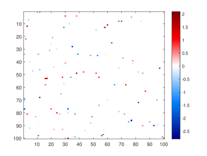
(b) Estimated regression matrix $\hat{\bm{\Gamma}}$

Figure 6: Comparison between the original regression coefficient matrix $\bm{\Gamma}_{\star}$ and its estimation $\hat{\bm{\Gamma}}$.

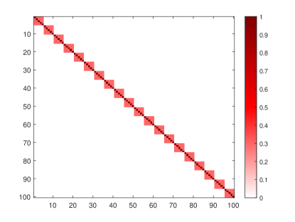
(a) Original precision matrix $\bm{\Omega}_{\star}$

(b) Estimated precision matrix $\hat{\bm{\Omega}}$

Figure 7: Comparison between the original precision matrix $\bm{\Omega}_{\star}$ and its estimation $\hat{\bm{\Omega}}$.

In Figure 6 and 7, we compare the original regression coefficient matrix $\bm{\Gamma}_{\star}$ and the precision matrix $\bm{\Omega}_{\star}$ with their estimations $\hat{\bm{\Gamma}}$ and $\hat{\bm{\Omega}}$ respectively. These figures illustrate that Algorithm 1 and our initialization (Algorithm 2) could recover the sparse structures of $\bm{\Gamma}_{\star}$ and $\bm{\Omega}_{\star}$, and verify our theoretical results. For Algorithm 3 and 4 with the $l_{1}$-norm, the results are similar and we do not include them in this manuscript.

References

- [1] M. Yuan, A. Ekici, Z. Lu, and R. Monteiro, “Dimension reduction and coefficient estimation in multivariate linear regression,” Journal of the Royal Statistical Society. Series B (Statistical Methodology), vol. 69, no. 3, pp. 329–346, 2007. [Online]. Available: http://www.jstor.org/stable/4623272
- [2] T. T. Cai, H. Li, W. Liu, and J. Xie, “Covariate-adjusted precision matrix estimation with an application in genetical genomics,” Biometrika, vol. 100, no. 1, pp. 139–156, nov 2012.
- [3] J. Chen, P. Xu, L. Wang, J. Ma, and Q. Gu, “Covariate adjusted precision matrix estimation via nonconvex optimization,” in Proceedings of the 35th International Conference on Machine Learning, ser. Proceedings of Machine Learning Research, J. Dy and A. Krause, Eds., vol. 80. Stockholmsmässan, Stockholm Sweden: PMLR, 10–15 Jul 2018, pp. 922–931. [Online]. Available: http://proceedings.mlr.press/v80/chen18n.html
- [4] P. Bühlmann and S. van de Geer, Statistics for High-Dimensional Data: Methods, Theory and Applications, 1st ed. Springer Publishing Company, Incorporated, 2011.
- [5] J. Lin, S. Basu, M. Banerjee, and G. Michailidis, “Penalized maximum likelihood estimation of multi-layered gaussian graphical models,” Journal of Machine Learning Research, vol. 17, no. 146, pp. 1–51, 2016. [Online]. Available: http://jmlr.org/papers/v17/16-004.html
- [6] S. Lauritzen, Graphical Models. Oxford New York: Clarendon Press Oxford University Press, 1996, vol. 17.
- [7] E. Segal, N. Friedman, N. Kaminski, A. Regev, and D. Koller, “From signatures to models: Understanding cancer using microarrays,” Nature Genetics, vol. 37, no. S6, pp. S38–S45, jun 2005.
- [8] N. Meinshausen and P. Bühlmann, “High-dimensional graphs and variable selection with the Lasso,” The Annals of Statistics, vol. 34, no. 3, pp. 1436–1462, jun 2006.
- [9] M. Yuan and Y. Lin, “Model selection and estimation in the gaussian graphical model,” Biometrika, vol. 94, no. 1, pp. 19–35, feb 2007.
- [10] J. Friedman, T. Hastie, and R. Tibshirani, “Sparse inverse covariance estimation with the graphical lasso,” Biostatistics, vol. 9, no. 3, pp. 432–441, dec 2007.
- [11] A. J. Rothman, P. J. Bickel, E. Levina, and J. Zhu, “Sparse permutation invariant covariance estimation,” Electronic Journal of Statistics, vol. 2, no. none, jan 2008.
- [12] P. Ravikumar, M. J. Wainwright, G. Raskutti, and B. Yu, “High-dimensional covariance estimation by minimizing 1-penalized log-determinant divergence,” Electronic Journal of Statistics, vol. 5, no. none, jan 2011.
- [13] G. Obozinski, M. J. Wainwright, and M. I. Jordan, “Support union recovery in high-dimensional multivariate regression,” The Annals of Statistics, vol. 39, no. 1, feb 2011.
- [14] V. G. Cheung and R. S. Spielman, “The genetics of variation in gene expression,” Nature Genetics, vol. 32, no. S4, pp. 522–525, dec 2002.
- [15] R. B. Brem and L. Kruglyak, “The landscape of genetic complexity across 5,700 gene expression traits in yeast,” Proceedings of the National Academy of Sciences, vol. 102, no. 5, pp. 1572–1577, jan 2005.
- [16] A. J. Rothman, E. Levina, and J. Zhu, “Sparse multivariate regression with covariance estimation,” Journal of Computational and Graphical Statistics, vol. 19, no. 4, pp. 947–962, jan 2010.
- [17] J. Yin and H. Li, “A sparse conditional Gaussian graphical model for analysis of genetical genomics data,” The Annals of Applied Statistics, vol. 5, no. 4, pp. 2630–2650, dec 2011.
- [18] W. Lee and Y. Liu, “Simultaneous multiple response regression and inverse covariance matrix estimation via penalized Gaussian maximum likelihood,” Journal of Multivariate Analysis, vol. 111, pp. 241–255, oct 2012.
- [19] K.-A. Sohn and S. Kim, “Joint estimation of structured sparsity and output structure in multiple-output regression via inverse-covariance regularization,” in Proceedings of the Fifteenth International Conference on Artificial Intelligence and Statistics, ser. Proceedings of Machine Learning Research, N. D. Lawrence and M. Girolami, Eds., vol. 22. La Palma, Canary Islands: PMLR, 21–23 Apr 2012, pp. 1081–1089. [Online]. Available: http://proceedings.mlr.press/v22/sohn12.html
- [20] X. Yuan and T. Zhang, “Partial gaussian graphical model estimation,” IEEE Transactions on Information Theory, vol. 60, no. 3, pp. 1673–1687, 2014.
- [21] C. McCarter and S. Kim, “On sparse gaussian chain graph models,” in Advances in Neural Information Processing Systems, Z. Ghahramani, M. Welling, C. Cortes, N. Lawrence, and K. Q. Weinberger, Eds., vol. 27. Curran Associates, Inc., 2014, pp. 3212–3220. [Online]. Available: https://proceedings.neurips.cc/paper/2014/file/81c650caac28cdefce4de5ddc18befa0-Paper.pdf
- [22] ——, “Large-scale optimization algorithms for sparse conditional gaussian graphical models,” in Proceedings of the 19th International Conference on Artificial Intelligence and Statistics, ser. Proceedings of Machine Learning Research, A. Gretton and C. C. Robert, Eds., vol. 51. Cadiz, Spain: PMLR, 09–11 May 2016, pp. 528–537. [Online]. Available: http://proceedings.mlr.press/v51/mccarter16.html
- [23] S. Chen and A. Banerjee, “Alternating estimation for structured high-dimensional multi-response models,” in Advances in Neural Information Processing Systems 30, I. Guyon, U. V. Luxburg, S. Bengio, H. Wallach, R. Fergus, S. Vishwanathan, and R. Garnett, Eds. Curran Associates, Inc., 2017, pp. 2838–2848. [Online]. Available: http://papers.nips.cc/paper/6876-alternating-estimation-for-structured-high-dimensional-multi-response-models.pdf
- [24] ——, “An improved analysis of alternating minimization for structured multi-response regression,” in Advances in Neural Information Processing Systems 31, S. Bengio, H. Wallach, H. Larochelle, K. Grauman, N. Cesa-Bianchi, and R. Garnett, Eds. Curran Associates, Inc., 2018, pp. 6616–6627. [Online]. Available: http://papers.nips.cc/paper/7896-an-improved-analysis-of-alternating-minimization-for-structured-multi-response-regression.pdf
- [25] S. Balakrishnan, M. J. Wainwright, and B. Yu, “Statistical guarantees for the EM algorithm: From population to sample-based analysis,” The Annals of Statistics, vol. 45, no. 1, pp. 77–120, feb 2017.
- [26] J. M. Klusowski, D. Yang, and W. D. Brinda, “Estimating the coefficients of a mixture of two linear regressions by expectation maximization,” IEEE Transactions on Information Theory, vol. 65, no. 6, pp. 3515–3524, 2019.
- [27] R. Sun and Z. Luo, “Guaranteed matrix completion via non-convex factorization,” IEEE Transactions on Information Theory, vol. 62, no. 11, pp. 6535–6579, 2016.
- [28] P. Jain, A. Tewari, and P. Kar, “On iterative hard thresholding methods for high-dimensional m-estimation,” in Proceedings of the 27th International Conference on Neural Information Processing Systems - Volume 1, ser. NIPS’14. Cambridge, MA, USA: MIT Press, 2014, p. 685–693.
- [29] P. Jain and P. Kar, “Non-convex optimization for machine learning,” Foundations and Trends® in Machine Learning, vol. 10, no. 3-4, pp. 142–336, 2017.
- [30] M. Rudelson and R. Vershynin, “Hanson-Wright inequality and sub-gaussian concentration,” Electronic Communications in Probability, vol. 18, no. 0, 2013.
- [31] R. Adamczak, “A note on the Hanson-Wright inequality for random vectors with dependencies,” Electronic Communications in Probability, vol. 20, no. 0, 2015.
- [32] R. Vershynin, High-Dimensional Probability: an Introduction with Applications in Data Science, ser. Cambridge Series in Statistical and Probabilistic Mathematics. Cambridge University Press, 2018.
- [33] G. Raskutti, M. J. Wainwright, and B. Yu, “Minimax rates of estimation for high-dimensional linear regression over -balls,” IEEE Transactions on Information Theory, vol. 57, no. 10, pp. 6976–6994, 2011.
- [34] S. Oymak and B. Hassibi, “Sharp MSE bounds for proximal denoising,” Foundations of Computational Mathematics, vol. 16, no. 4, pp. 965–1029, oct 2015.
- [35] S. Oymak, B. Recht, and M. Soltanolkotabi, “Sharp time–data tradeoffs for linear inverse problems,” IEEE Trans. Inf. Theory, vol. 64, no. 6, pp. 4129–4158, 2018.
- [36] V. Chandrasekaran and M. I. Jordan, “Computational and statistical tradeoffs via convex relaxation,” Proceedings of the National Academy of Sciences, vol. 110, no. 13, pp. E1181–E1190, 2013.
- [37] D. Amelunxen, M. Lotz, M. McCoy, and J. Tropp, “Living on the edge: Phase transitions in convex programs with random data,” Information and Inference, vol. 3, 03 2013.
- [38] T. T. Cai, W. Liu, and H. H. Zhou, “Estimating sparse precision matrix: Optimal rates of convergence and adaptive estimation,” The Annals of Statistics, vol. 44, no. 2, pp. 455–488, apr 2016.
- [39] M. Talagrand, The Generic Chaining. Springer-Verlag GmbH, 2005. [Online]. Available: https://www.ebook.de/de/product/3271874/michel_talagrand_the_generic_chaining.html
- [40] C. Nugent, “S&p 500 stock data,” https://www.kaggle.com/camnugent/sandp500, 2018, version 4.
- [41] J. Fan, A. Furger, and D. Xiu, “Incorporating global industrial classification standard into portfolio allocation: A simple factor-based large covariance matrix estimator with high-frequency data,” Journal of Business & Economic Statistics, vol. 34, no. 4, pp. 489–503, sep 2016.
- [42] A. Skripnikov and G. Michailidis, “Joint estimation of multiple network Granger causal models,” Econometrics and Statistics, vol. 10, pp. 120–133, apr 2019.
- [43] S. Dirksen, “Tail bounds via generic chaining,” Electronic Journal of Probability, vol. 20, no. 0, 2015.
- [44] X. Li, T. Zhao, R. Arora, H. Liu, and J. Haupt, “Stochastic variance reduced optimization for nonconvex sparse learning,” in Proceedings of The 33rd International Conference on Machine Learning, ser. Proceedings of Machine Learning Research, M. F. Balcan and K. Q. Weinberger, Eds., vol. 48. New York, New York, USA: PMLR, 20–22 Jun 2016, pp. 917–925. [Online]. Available: http://proceedings.mlr.press/v48/lid16.html
- [45] Y. Nesterov, Introductory Lectures on Convex Optimization: A Basic Course, 1st ed. Springer Publishing Company, Incorporated, 2014.
- [46] N. M. N. Boris S. Mordukhovich, An Easy Path to Convex Analysis and Applications. Morgan & Claypool Publishers, 2013. [Online]. Available: https://www.ebook.de/de/product/21948390/boris_s_mordukhovich_nguyen_mau_nam_an_easy_path_to_convex_analysis_and_applications.html
- [47] I. Melnyk and A. Banerjee, “Estimating structured vector autoregressive models,” in Proceedings of the 33rd International Conference on International Conference on Machine Learning - Volume 48, ser. ICML’16. JMLR.org, 2016, p. 830–839.