ReLU Deep Neural Networks from
the Hierarchical Basis Perspective

Abstract

We study ReLU deep neural networks (DNNs) by investigating their connections with the hierarchical basis method in finite element methods. First, we show that the approximation schemes of ReLU DNNs for $x^{2}$ and $xy$ are composition versions of the hierarchical basis approximation for these two functions. Based on this fact, we obtain a geometric interpretation and systematic proof for the approximation result of ReLU DNNs for polynomials, which plays an important role in a series of recent exponential approximation results of ReLU DNNs. Through our investigation of connections between ReLU DNNs and the hierarchical basis approximation for $x^{2}$ and $xy$, we show that ReLU DNNs with this special structure can be applied only to approximate quadratic functions. Furthermore, we obtain a concise representation to explicitly reproduce any linear finite element function on a two-dimensional uniform mesh by using ReLU DNNs with only two hidden layers.

1 Introduction

Models based on artificial neural networks (ANNs) have achieved unexpected success in a wide range of machine learning and artificial intelligence fields such as computer vision, natural language processing, and reinforcement learning [19, 7]. Mathematical analysis of ANNs can be carried out using many different approaches, including via the popular approximation and representation theory of ANNs, which is critical to developing a mathematical understanding of these models. From the 1990s onward, researchers have studied approximation properties for single hidden layer neural networks as in [14, 4, 16, 2, 20, 6, 32, 17, 34, 37, 35, 22]. However, the results of several recent studies [18, 12, 15] indicate that compared with neural networks with one hidden layer, those with more hidden layers – referred as “deep neural networks (DNNs)” – can achieve much better performance. These results motivate further exploration of the approximation and expression theory of DNNs. Specifically, it is natural to ask how the depth in DNNs affects and contributes to the approximation performance and expressive power.

Generally speaking, DNNs with any non-polynomial activation function can demonstrate what has come to be known as “universal approximation ability”  [20, 34]. However, of the activation functions available, the rectified linear unit [29] activation function ${\rm ReLU(x)}=\max\{0,x\}$ is the most successful and, therefore, also the most popular. The main reason for its success is twofold: Not only can ReLU DNNs achieve state-of-the-art performance in practice, but they also show rich mathematical structures and properties in theory. Thus, understanding and interpreting the approximation efficacy of ReLU DNNs has become a crucial topic, as evidenced by a growing body of literature [28, 36, 33, 38, 24, 5, 26, 27, 21, 9, 25]. From the viewpoint of representation properties, two notable results [28, 36] show that ReLU DNNs can produce complicated continuous piece-wise linear functions whose number of linear regions grows as the power of the number of layers. Then, [38] established the first exponential approximation rate for a general function class through the use of ReLU DNN with limited width, by discovering an elegant approximation property for the square function $s(x)=x^{2}$ on $[-1,1]$ employing ReLU DNNs. In the wake of that discovery, numerous research studies have been published in which various exponential error bounds are developed for classical or modified ReLU DNNs for different function families or measurements. For example, [24] introduced a new and more uniform network architecture to achieve these results in [38]. Then, [5] further improved the network structure by involving architecture similar to that of ResNet [12, 13], thereby obtaining an exponential convergence rate for a special class of analytic function. [26, 27, 21] investigated the approximation properties on Koborov space, bandlimited functions, and $C^{s}$ functions by approximating sparse grids, truncated Chebyshev series, and Taylor expansions. A series of results [30, 31, 9, 25] for different function spaces and norms have been obtained by combining approximation properties in finite element methods. Although numerous results have been achieved based on the crucial approximation result of ReLU DNN for the square function $s(x)=x^{2}$, the field still lacks the in-depth understanding needed to extend this special result.

In this paper, we will first concentrate on understanding and interpreting the approximation properties of ReLU DNNs for both the square function $s(x)=x^{2}$ and the multiplication function $m(x,y)=xy$ from the hierarchical basis perspective [3, 8]. Briefly, our main discovery is that the ReLU DNN approximation for $s(x)=x^{2}$ is actually the hierarchical basis approximation for $x^{2}$ with a composition scheme. This observation provides a completely new viewpoint from which to understand the ReLU DNN approximation for $x^{2}$. At the same time, it will greatly simplify the proof developed in [38] and lead to a more precise error estimation. Based on these results, we prove that only quadratic functions can be efficiently approximated with a special ReLU DNN architecture. Through a further investigation of the ReLU DNN approximation for $m(x,y)=xy$ from the hierarchical basis viewpoint, we find a geometric interpretation for the result reported in [38] originally derived from the pure algebraic relation. According to this new understanding and interpretation of the approximation properties of ReLU DNNs for $s(x)=x^{2}$ and $m(x,y)=xy$ from the viewpoint of hierarchical basis and finite element interpolation, we achieve some more accurate and tighter error estimations about the approximation results of ReLU DNNs for polynomials with multi-variables that are than the results in [38, 5, 26, 27]. Furthermore, we achieve a very unexpected and important result from our study of the connections between ReLU DNNs in relation to the hierarchical basis method: that is, we obtain an explicit and concise formula to represent any linear finite element function on uniform mesh on $\mathbb{R}^{2}$ with only two hidden layers, which is generally considered to be not trivial and very complicated as discussed in [1, 11].

This paper is organized as follows. In Section 2, we will introduce some notations and preliminary results for ReLU DNNs. In Section 3, we account for the approximation properties of ReLU DNNs for the square function $s(x)=x^{2}$ by using the hierarchical basis method and show that only quadratic functions can achieve an exponential approximation rate under a specific ReLU DNN architecture. In Section 4, we draw on these same techniques to study the multiplication function $m(x,y)=xy$ in order to meet two related goals: (i) to capture some further approximation and expressive properties of ReLU DNNs for $m(x,y)$, and (ii) to obtain tighter error estimations for approximating multi-variable polynomials. In Section 5, we present a detailed account of our unexpected discovery from the previous investigation of $m(x,y)$. Specifically, we show how to represent a finite element function with uniform mesh on 2D by using ReLU DNNs with only two hidden layers. In Section 6, we offer some concluding remarks.

2 Preliminary results of ReLU DNNs

In this section, we will briefly discuss the definition and properties of the DNNs generated by using the ReLU activation function.

2.1 The classical DNN with ReLU activation function

First, we introduce the general plain DNN function $f:\mathbb{R}^{d}\to\mathbb{R}^{c}$ with L hidden layers by

$$\begin{cases}f^{\ell}(x)&=\sigma\circ\theta^{\ell}(f^{\ell-1}(x))\quad\ell=1:L\\ f(x)&=\theta^{L+1}(f^{L}(x))\end{cases},$$ (2.1)

with $f^{0}(x)=x$ where

$$\theta^{\ell}:\mathbb{R}^{n_{\ell-1}}\to\mathbb{R}^{n_{\ell}},$$ (2.2)

is the (vector) linear function defined by

$$\theta^{\ell}(x)=W^{\ell}x+b^{\ell},$$ (2.3)

where $W^{\ell}=(w^{\ell}_{ij})\in\mathbb{R}^{n_{\ell}\times n_{\ell-1}}$, $b^{\ell}\in\mathbb{R}^{n_{\ell}}$.

In the above definition, we denote the nonlinear activation function as

$$\sigma:\mathbb{R}\to\mathbb{R}.$$ (2.4)

By applying the function to each component, we can extend this naturally to

$$\sigma:\mathbb{R}^{n}\mapsto\mathbb{R}^{n}.$$ (2.5)

Given $d,L\in\mathbb{N}^{+}$ and

$$n_{1:L}=(n_{1},\dots,n_{L})\in(\mathbb{N}^{+})^{L}\mbox{ with }n_{0}=d,n_{L+1}=1,$$ (2.6)

the general DNN from $\mathbb{R}^{d}$ to $\mathbb{R}$ defined above is denoted by

$$\mathcal{N}_{n_{1:L}}:=\{f:f(x)=\theta^{L+1}\circ\sigma\circ\theta^{L}\circ\sigma\cdots\circ\theta^{2}\circ\sigma\circ\theta^{1}(x)\}.$$ (2.7)

A DNN of this kind, referred to as an $(L+1)$-layer DNN, is said to have $L$ hidden layers. Unless stated otherwise, the term “layer” should always be taken to mean “hidden layer” in the rest of this paper. The size of this DNN is $n_{1}+\cdots+n_{L}$. For the activation functions, in this paper, we focus on considering a special activation function, known as the “rectified linear unit” (ReLU), and defined as $\mbox{{\rm ReLU}}:\mathbb{R}\mapsto\mathbb{R}$,

$$\mbox{{\rm ReLU}}(x)=\max(0,x),\quad x\in\mathbb{R}.$$ (2.8)

A ReLU DNN with $L$ hidden layers might be written as

$$f(x)=\theta^{L+1}\circ\mbox{{\rm ReLU}}\circ\theta^{L}\circ\mbox{{\rm ReLU}}\cdots\circ\theta^{2}\circ\mbox{{\rm ReLU}}\circ\theta^{1}(x).$$ (2.9)

Furthermore, if $n_{1:L}=(N,N,\cdots,N)$ we denote

$$\mathcal{N}_{n_{1:L}}:=\mathcal{N}_{L}^{N},$$ (2.10)

for simplicity.

2.2 A class of ResNet-type ReLU DNNs

In this subsection, we will introduce a class of specific ReLU DNNs with some special short-cut connections, as described in [38, 5].

Following an idea similar to that above, for any $n_{1:L}=(n_{1},\dots,n_{L})\in(\mathbb{N}^{+})^{L}\mbox{ with }n_{0}=d,n_{L+1}=1$, we define the next ReLU DNN with special short-cut connections:

$$\begin{cases}f^{1}(x)&=\sigma\circ\widehat{\theta}^{1}(x)\\ f^{\ell}(x)&=\sigma\circ\widehat{\theta}^{\ell}([x,f^{\ell-1}(x)])\quad\ell=2:L\\ f(x)&=\widehat{\theta}^{L+1}([x,f^{1},\cdots,f^{L}])\\ \end{cases}.$$ (2.11)

Here, we have $[x,f^{\ell-1}(x)]\in\mathbb{R}^{d+n_{\ell-1}}$ for $\ell=2:L$, $[x,f^{1},\cdots,f^{L}]\in\mathbb{R}^{\sum_{i=0}^{L}n_{i}}$ and $f^{\ell}\in\mathbb{R}^{n_{\ell}}$ for $\ell=1:L$. In addition, we note that $\widehat{\theta}^{\ell}$ is an affine mapping to $\mathbb{R}^{n_{\ell}}$. Furthermore, we denote the above function class as $\widehat{\mathcal{N}}_{n_{1:L}}$ and

$$\widehat{\mathcal{N}}_{L}^{N}=\widehat{\mathcal{N}}_{n_{1:L}},$$ (2.12)

if $n_{1:L}=(N,N,\cdots,N)$. It is easy to see that this function class is quite different from the standard ReLU DNN models. For $\widehat{\mathcal{N}}_{L}^{N}$, it always needs the original input data $x$ to be the input for all hidden layers. In addition, the last output layer of $\widehat{\mathcal{N}}_{L}^{N}$ collects outputs from all hidden layers and then make a linear combination. Fig. 2.1 shows more intuitive differences between $\mathcal{N}_{L}^{N}$ and $\widehat{\mathcal{N}}_{L}^{N}$ where $L=3$ and $N=2$.

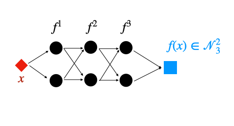
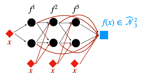
Figure 2.1: Diagrams for $\mathcal{N}_{3}^{2}$ (left) and $\widehat{\mathcal{N}}_{3}^{2}$ (right).

Given the ReLU function whereby

$$x=\mbox{{\rm ReLU}}(x)-\mbox{{\rm ReLU}}(-x),$$ (2.13)

we can, however, reconstruct the special ReLU DNN model $\widehat{\mathcal{N}}_{L}^{N}$ from the standard ReLU DNN model as shown in the following Lemma.

Lemma 2.1

(Connection between $\widehat{\mathcal{N}}_{L}^{N}$ and ${\mathcal{N}}_{L}^{M}$) For the fixed-width case, we have the next connection:

$$\widehat{\mathcal{N}}_{L}^{N}\subset{{\mathcal{N}}}_{L}^{N+2(d+1)}.$$ (2.14)

Proof  Assume that $\widehat{f}\in\widehat{{\mathcal{N}}}_{L}^{N}$. This means that there exist $\widehat{\theta}^{\ell}$ for $\ell=1:L+1$ such that

$$\widehat{f}=\widehat{\theta}^{L+1}([x,\widehat{f}^{1},\cdots,\widehat{f}^{L}])=\sum_{\ell=0}^{L}[\widehat{\theta}^{L+1}]_{\ell}(\widehat{f}^{\ell}),$$ (2.15)

where $\widehat{f}^{0}=x$, $\widehat{f}^{1}=\sigma\circ\widehat{\theta}^{1}(x)$ and

$$\widehat{f}^{\ell}=\sigma\circ\widehat{\theta}^{\ell}([x,\widehat{f}^{\ell-1}])=\sigma([\widehat{\theta}^{\ell}]_{x}(x)+[\widehat{\theta}^{\ell}]_{f}(\widehat{f}^{\ell-1})),$$ (2.16)

as defined in (2.11). Then, we can construct a function $f\in{{\mathcal{N}}}_{L}^{N+2(d+1)}$ such that

$$f^{1}=\sigma\circ\begin{pmatrix}\widehat{\theta}^{1}(x)\\ x\\ -x\\ [\widehat{\theta}^{L+1}]_{0}(x)\\ -[\widehat{\theta}^{L+1}]_{0}(x)\end{pmatrix}\in\mathbb{R}^{N+2(d+1)},$$ (2.17)

and

$$f^{\ell}=\sigma\circ\begin{pmatrix}[\widehat{\theta}^{\ell}]_{f}\left([f^{\ell-1}]_{1:N}\right)+[\widehat{\theta}^{\ell}]_{x}\left([f^{\ell-1}]_{N+1:N+d}-[f^{\ell-1}]_{N+d+1:N+2d}\right)\\ [f^{\ell-1}]_{N+1:N+d}-[f^{\ell-1}]_{N+d+1:N+2d}\\ -\left([f^{\ell-1}]_{N+1:N+d}-[f^{\ell-1}]_{N+d+1:N+2d}\right)\\ [\widehat{\theta}^{L+1}]_{\ell-1}([f^{\ell-1}]_{1:N})+[f^{\ell-1}]_{N+2d+1}-[f^{\ell-1}]_{N+2(d+1)}\\ -\left([\widehat{\theta}^{L+1}]_{\ell-1}([f^{\ell-1}]_{1:N})+[f^{\ell-1}]_{N+2d+1}-[f^{\ell-1}]_{N+2(d+1)}\right)\end{pmatrix}\in\mathbb{R}^{N+2(d+1)},$$ (2.18)

for all $\ell=2:L$. By recursion, we have

$$f^{\ell}=\sigma\circ\begin{pmatrix}\widehat{\theta}^{\ell}([x,\widehat{f}^{\ell-1}])\\ x\\ -x\\ \sum_{i=0}^{\ell-1}[\widehat{\theta}^{L+1}]_{i}(\widehat{f}^{i})\\ -\left(\sum_{i=0}^{\ell-1}[\widehat{\theta}^{L+1}]_{i}(\widehat{f}^{i})\right)\end{pmatrix}\in\mathbb{R}^{N+2(d+1)},$$ (2.19)

for all $\ell=2:L$. Then, we finish the proof by choosing the following special $\theta^{L+1}$ such that

$$f =\theta^{L+1}(f^{L})$$ (2.20)

$$=[\widehat{\theta}^{L+1}]_{L}([f^{L}]_{1:N})-[f^{L}]_{N+2d+1}+[f^{L}]_{N+2(d+1)}$$

$$=[\widehat{\theta}^{L+1}]_{L}(\widehat{f}^{L})+\sigma\left(\sum_{i=0}^{L-1}[\widehat{\theta}^{L+1}]_{i}(\widehat{f}^{i})\right)-\sigma\left(-\sum_{i=0}^{L-1}[\widehat{\theta}^{L+1}]_{i}(\widehat{f}^{i})\right)$$

$$=\sum_{\ell=0}^{L}[\widehat{\theta}^{L+1}]_{\ell}(\widehat{f}^{\ell})=\widehat{f}.$$

$\square$

The properties described next play a crucial role in the structure and approximation properties of $\widehat{{\mathcal{N}}}_{L}^{N}$, which can also be found in [5].

Properties 2.1

(Addition and composition of $\widehat{{\mathcal{N}}}_{L}^{N}$)

• Addition

  $$\widehat{{\mathcal{N}}}_{L_{1}}^{N}+\widehat{{\mathcal{N}}}_{L_{2}}^{N}\subseteq\widehat{{\mathcal{N}}}_{L_{1}+L_{2}}^{N},$$

  i.e., if $f_{1}\in\widehat{{\mathcal{N}}}_{L_{1}}^{N}$ and $f_{2}\in\widehat{{\mathcal{N}}}_{L_{2}}^{N}$, then $f_{1}+f_{2}\in\widehat{{\mathcal{N}}}_{L_{1}+L_{2}}^{N}$.

• Modified composition

  $$\widehat{{\mathcal{N}}}_{L_{2}}^{N+1}\diamond\widehat{{\mathcal{N}}}_{L_{1}}^{N}\subseteq\widehat{{\mathcal{N}}}_{L_{1}+L_{2}}^{N+1}.$$

  Here, if $f_{1}(x)\in\widehat{{\mathcal{N}}}_{L_{1}}^{N}$ and $f_{2}(x_{0},x)\in\widehat{{\mathcal{N}}}_{L_{2}}^{N+1}$ with $x_{0}\in\mathbb{R}$, then the modified composition is defined by

  $$f_{2}\diamond f_{1}=f_{2}(f_{1}(x),x).$$ (2.21)

  Then, the above property means that

  $$f_{2}\diamond f_{1}=f_{2}(f_{1}(x),x)\in\widehat{{\mathcal{N}}}_{L_{1}+L_{2}}^{N+1}.$$ (2.22)

Proof  For the addition property, if $f\in\widehat{{\mathcal{N}}}_{L_{1}}^{N}$ and $g\in\widehat{{\mathcal{N}}}_{L_{2}}^{N}$, we first construct $h\in\widehat{{\mathcal{N}}}_{L_{1}+L_{2}}^{N}$ with

$$h_{\ell}(x)=f_{\ell}(x),\quad\text{for}\quad\ell=1:L_{1}.$$ (2.23)

Because the input of $h_{L_{1}+1}$ includes the original input $x$ directly as in the definition of $\widehat{{\mathcal{N}}}_{L_{1}+L_{2}}^{N}$ in (2.11), we define

$$h_{L_{1}+1}(x)=\widehat{\theta}_{h}^{L_{1}+1}([x,h_{L_{1}}(x)])=\widehat{\theta}_{g}^{1}(x)=g_{1}(x).$$ (2.24)

Then, we can construct

$$h_{L_{1}+\ell}(x)=g_{\ell}(x),\quad\text{for}\quad\ell=2:L_{2}.$$ (2.25)

Finally, we obtain

$$h(x) =\widehat{\theta}_{h}^{L_{1}+L_{2}+1}([x,h_{1},\cdots,h_{L_{1}+L_{2}}])$$ (2.26)

$$=\widehat{\theta}_{f}^{L_{1}+1}([x,h_{1},\cdots,h_{L_{1}}])+\widehat{\theta}_{g}^{L_{2}+1}([x,h_{L_{1}+1},\cdots,h_{L_{1}+L_{2}}])$$

$$=\widehat{\theta}_{f}^{L_{1}+1}([x,f_{1},\cdots,f_{L_{1}}])+\widehat{\theta}_{g}^{L_{2}+1}([x,g_{1},\cdots,g_{L_{2}}])$$

$$=f(x)+g(x).$$

Then, the modified composition property can be directly proved by the definition of $\widehat{{\mathcal{N}}}_{L}^{N}$ in (2.11). $\square$

From the proofs of Lemma 2.1 and Properties 2.1, we can see that the skip connection structure ($f^{\ell}(x)=\sigma\circ\widehat{\theta}^{\ell}([x,f^{\ell-1}(x)])$) in (2.11), which differs from the skip connection in the classical ResNet [12, 13], is essential to guaranteeing the previous lemma and properties.

3 ReLU DNN and hierarchical basis for the function $x^{2}$

In this section, we begin by discussing the hierarchical basis [8] and the DNN approximation for the function $s(x)=x^{2}$. Then, we show that $s(x)=x^{2}$ is the unique function which can be directly approximated by composition from the hierarchical basis viewpoint.

3.1 ReLU DNN approximation of $x^{2}$: A hierarchical basis interpretation

We consider a set of equidistant grids $\mathcal{T}_{\ell}$ for level $\ell\geq 0$ on the unit interval $\bar{\Omega}=[0,1]$ with mesh size $h_{\ell}=2^{-\ell}$. Here, we denote grid $\mathcal{T}_{\ell}$ as

$$\mathcal{T}_{\ell}:=\left\{\left.x_{\ell,i}~{}\right|~{}x_{\ell,i}=ih_{\ell},~{}0\leq i\leq 2^{\ell}\right\}.$$ (3.1)

At grid point $x_{\ell,i}$, the nodal basis function $\phi_{\ell,i}(x)$ on $\mathcal{T}_{\ell}$ is defined as

$$\phi_{\ell,i}(x):=g\left(\frac{x-(i-1)h_{\ell}}{2h_{\ell}}\right)\quad x\in\mathbb{R},$$ (3.2)

where

$$g(x)=\begin{cases}2x,\quad&x\in\left[0,\frac{1}{2}\right],\\ 2(1-x),\quad&x\in\left(\frac{1}{2},1\right],\\ 0,\quad&\text{others}.\end{cases}$$ (3.3)

By definition, we have $\phi_{1,1}(x)=g(x)$. In addition, for $\ell=0$, we have these two basis functions,

$$\phi_{0,0}=1-x\quad\text{and}\quad\phi_{0,1}=x,\quad\text{for }x\in[0,1].$$ (3.4)

These basis functions are used to define the piecewise linear function space

$$V_{\ell}:=\mbox{span}\{\phi_{\ell,i}:0\leq i\leq 2^{\ell}\}\subset H^{1}(0,1),\quad\ell\geq 0.$$ (3.5)

Then, let us define the the piecewise linear interpolation on $\mathcal{T}_{\ell}$ as:

$$I_{\ell}u=\sum_{i=0}^{2^{\ell}}u(x_{\ell,i})\phi_{\ell,i}.$$ (3.6)

Thus, we have the next hierarchical decomposition for $L\geq 1$:

$$I_{L}u=I_{0}u+\sum_{\ell=1}^{L}(I_{\ell}-I_{\ell-1})u=I_{0}u+\sum_{\ell=1}^{L}\sum_{i\in\mathcal{I}_{\ell}}\mu_{\ell,i}\phi_{\ell,i},$$ (3.7)

where

$$\mathcal{I}_{\ell}=\{i\in\mathbb{N}~{}:~{}1\leq i\leq 2^{\ell}-1,~{}i~{}\text{ is odd}\}.$$ (3.8)

Furthermore, we have

$$(I_{\ell}-I_{\ell-1})u=\sum_{i\in\mathcal{I}_{\ell}}\mu_{\ell,i}\phi_{\ell,i}=\sum_{i\in\mathcal{I}_{\ell}}\left(u(x_{\ell,i})-\frac{1}{2}\left(u(x_{\ell,i-1})+u(x_{\ell,i+1})\right)\right)\phi_{\ell,i}.$$ (3.9)

The key observation is that there exists a special decomposition form once we take $u(x)=s(x)=x^{2}$. By the hierarchical decomposition above, we have

$$(I_{\ell}-I_{\ell-1})s(x) =\sum_{i\in\mathcal{I}_{\ell}}\left(s(x_{\ell,i})-\frac{1}{2}\left(s(x_{\ell,i-1})+s(x_{\ell,i+1})\right)\right)\phi_{\ell,i}(x)$$ (3.10)

$$=\sum_{i\in\mathcal{I}_{\ell}}\left(x_{\ell,i}^{2}-\frac{1}{2}(x_{\ell,i-1}^{2}+x_{\ell,i+1}^{2})\right)\phi_{\ell,i}(x)$$

$$=\sum_{i\in\mathcal{I}_{\ell}}\left(x_{\ell,i}^{2}-\frac{1}{2}\left((x_{\ell,i}-h_{\ell})^{2}+(x_{\ell,i}+h_{\ell})^{2}\right)\right)\phi_{\ell,i}(x)$$

$$=-h_{\ell}^{2}\sum_{i\in\mathcal{I}_{\ell}}\phi_{\ell,i}(x).$$

Given that $I_{0}s=s(0)\phi_{0,0}+s(1)\phi_{0,1}=x$ on $[0,1]$, we have

$$I_{L}s(x)=I_{0}s(x)+\sum_{\ell=1}^{L}(I_{\ell}-I_{\ell-1})s(x)=x-\sum_{\ell=1}^{\ell}h^{2}_{\ell}\sum_{i\in\mathcal{I}_{\ell}}\phi_{\ell,i}(x)=x-\sum_{\ell=1}^{\ell}h^{2}_{\ell}g_{\ell}(x),$$ (3.11)

where

$$g_{\ell}(x):=\sum_{i\in\mathcal{I}_{\ell}}\phi_{\ell,i}(x).$$ (3.12)

By definition, we have the following diagram of $g_{\ell}(x)$:

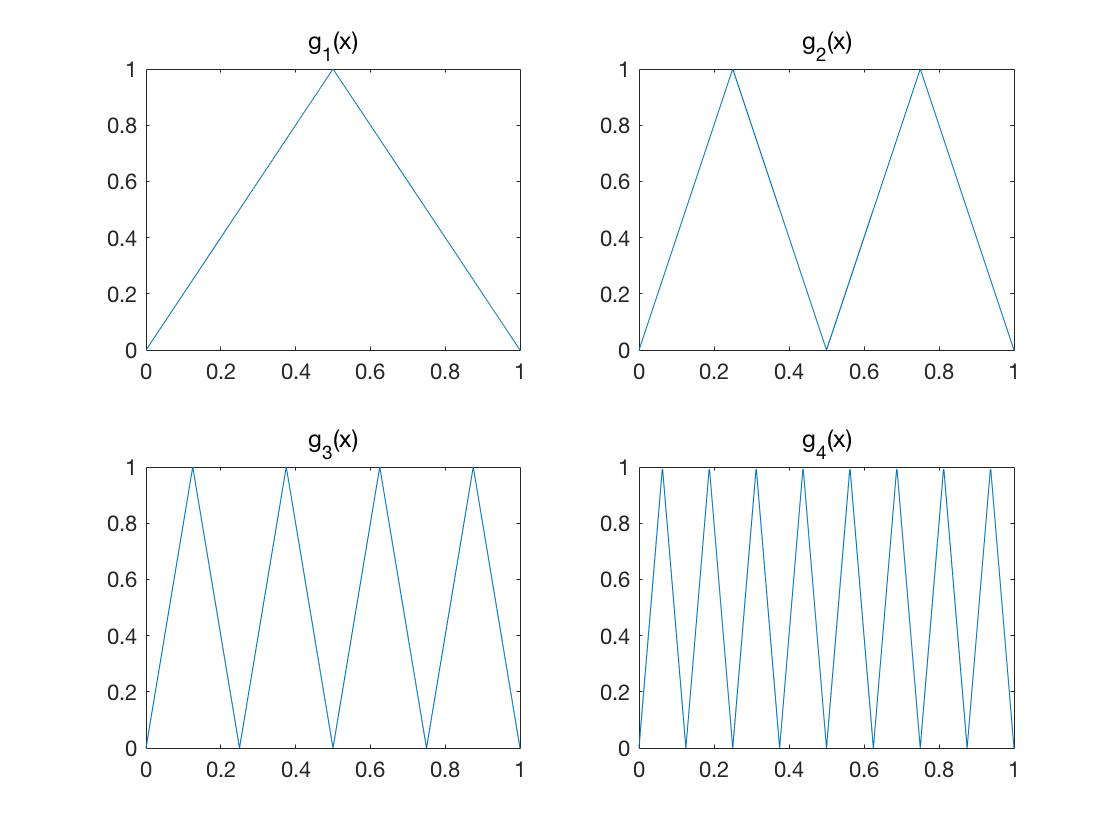
Figure 3.1: Representations of $g_{\ell}(x)$ for $\ell=1,2,3,4$.

The next property plays a crucial role in the connections between ReLU DNNs and the hierarchical basis functions:

$$g_{\ell}(x)=g(g_{\ell-1}(x))$$ (3.13)

for $\ell=2,...,L$ where $g_{1}(x)=g(x)$ as defined in (3.3). Based on the connections between the linear finite element functions and the ReLU DNNs as in [11], we actually have

$$g(x)=2\mbox{{\rm ReLU}}(x)-4\mbox{{\rm ReLU}}({x-\frac{1}{2}})+2\mbox{{\rm ReLU}}(x-1)\in{{\mathcal{N}}}_{1}^{3}$$ (3.14)

for any $x\in\mathbb{R}$. Thus, we have the next key observation,

$$g_{\ell}\in{\mathcal{N}}_{\ell}^{3},$$ (3.15)

because of the composition structure. Based on the definition of $\widehat{{\mathcal{N}}}_{\ell}^{3}$, the above relation leads to

$$x-\sum_{\ell=1}^{L}h^{2}_{\ell}g_{\ell}(x)\in\widehat{{\mathcal{N}}}_{L}^{3}.$$ (3.16)

Before we show the approximation result for $s(x)=x^{2}$ by using an ReLU DNN, we recall the interpolation error estimates of $I_{L}s$ for the $L^{\infty}$ and $W^{1,\infty}$ norms.

Lemma 3.1

If $s(x)=x^{2}$, then we have the next approximation results for $I_{L}$

$$\|s-I_{L}s\|_{L^{\infty}([0,1])}=2^{-2(L+1)}\quad\text{and}\quad|s-I_{L}s|_{W^{1,\infty}(0,1)}\leq 2^{-L}.$$ (3.17)

Based on the lemma above, we will show a new and concise proof of the next theorem.

Theorem 3.1

For function $s(x)=x^{2}$, there exists $\hat{s}_{L}(x)\in\widehat{{\mathcal{N}}}_{L}^{3}$ such that:

$$\|\hat{s}_{L}-s\|_{L^{\infty}([-1,1])}=2^{-2L}\quad\text{and}\quad|\hat{s}_{L}-s|_{W^{1,\infty}(-1,1)}\leq 2^{-(L-1)}.$$ (3.18)

Proof  We first define

$$s_{L-1}(x)=I_{L-1}s(x)=x-\sum_{l=1}^{L-1}\frac{g_{\ell}(x)}{2^{2\ell}}\in\widehat{{\mathcal{N}}}_{L-1}^{3}.$$ (3.19)

Then, we construct the function

$$\hat{s}_{L}(x)=s_{L-1}(|x|)=s_{L-1}(\mbox{{\rm ReLU}}(x)+\mbox{{\rm ReLU}}(-x))\in\widehat{{\mathcal{N}}}_{L}^{3}.$$ (3.20)

Thus, we have

$$\hat{s}_{L}(x)=\begin{cases}I_{L-1}s(-x),\quad&x\in[-1,0]\\ I_{L-1}s(x),\quad&x\in(0,1]\end{cases},$$ (3.21)

where $I_{L-1}$ is the uniform interpolation with mesh size $h_{L-1}=(\frac{1}{2})^{L-1}$ on $[0,1]$ as defined in (3.6). According to the construction of $I_{L-1}s(x)$ and the symmetry of $s(x)=x^{2}$, we have

$$\sup_{x\in[-1,0]}|s(x)-I_{L-1}s(-x)|=\sup_{x\in[0,1]}|s(x)-I_{L-1}s(x)|,$$ (3.22)

which leads to

$$\|s-\hat{s}_{L}\|_{L^{\infty}([-1,0])}=||s-\hat{s}_{L}||_{L^{\infty}([0,1])}.$$ (3.23)

Finally, we have the next estimate for the $L^{\infty}$ norm:

$$||s-\hat{s}_{L}||_{L^{\infty}([-1,1])} =\max\left\{\|s-\hat{s}_{L}\|_{L^{\infty}([-1,0])},\|s-\hat{s}_{L}\|_{L^{\infty}([0,1])}\right\}$$ (3.24)

$$=\|s-\hat{s}_{L}\|_{L^{\infty}([0,1])}=||s-I_{L-1}s||_{L^{\infty}([0,1])}=2^{-2L}.$$

Following a similar argument, we can get the result for the $W^{1,\infty}(-1,1)$ norm. $\square$

The result for the $L^{\infty}$ norm was introduced in [38] and then developed in [5] for $\widehat{{\mathcal{N}}}_{L}^{3}$. Based on the definition of $\hat{s}_{L}(x)$ in (3.20), we have

$$\hat{s}_{L}(x)={} x_{L-1,i}^{2}\frac{x_{L-1,i}+h_{L-1}-x}{h_{L-1}}+(x_{L-1,i}+h_{L-1})^{2}\frac{x-x_{L-1,i}}{h_{L-1}}$$ (3.25)

$$={} (2x_{L-1,i}+h_{L-1})x-x_{L-1,i}(x_{L-1,i}+h_{L-1})$$

for any $x\in[x_{L-1,i},x_{L-1,i}+h_{L-1}]$ and $x_{L-1,i}$ (or $-x_{L-1,i}$) in grid points $\mathcal{T}_{L-1}$, as defined in (3.1). That is, $\hat{s}_{L}(x)$ equals the uniform interpolation for $s(x)$ on $[-1,1]$ with mesh size $h_{L-1}=2^{1-L}$. This account, therefore, provides a geometrical interpretation for $\hat{s}_{L}(x)$ and a new understanding of this approximation property.

3.2 Can the super-approximation result of ReLU DNNs for $x^{2}$ be extended?

As discussed, the key connection between the ReLU DNN and hierarchical basis method is the special non-local “basis” function $g_{\ell}\in{\mathcal{N}}_{L}^{3}$. Here, a natural idea to extend this connection is to study the representation power of the space spanned by $\{g_{\ell}\}_{\ell=1}^{\infty}$ in $H^{1}(0,1)$. For example, if

$$u=\sum_{\ell=1}^{\infty}\mu_{\ell}g_{\ell},$$ (3.26)

then we can apply the following approximation scheme:

$$u\approx\sum_{\ell=1}^{L}\mu_{\ell}g_{\ell}\in\widehat{{\mathcal{N}}}_{L}^{3}.$$ (3.27)

That is, we can achieve some efficient approximation results using $\widehat{{\mathcal{N}}}_{L}^{3}$ for any $u\in U$ if $U={\rm span}\{g_{1},g_{2},\cdots\}$ forms a nontrivial and rich subset of $H_{0}^{1}(0,1)$.

However, the next theorem shows that $u(x)$ can only be a quadratic function if $u(x)$ is spanned by $\{g_{\ell}\}_{\ell=1}^{\infty}$ with certain regularity assumption, for example $u(x)\in C^{3}(0,1)$.

Theorem 3.2

If $u\in C^{3}(0,1)$ and

$$u=I_{0}u+\sum_{\ell=1}^{\infty}\sum_{i\in\mathcal{I}_{\ell}}\mu_{\ell}\phi_{\ell,i},$$ (3.28)

then, $u(x)$ must be a quadratic function.

Proof  Without loss of generality, let us consider $u(0)=u(1)=0$. Otherwise, we can subtract the linear interpolation of the original function with boundary values. That is, we have

$$u=\sum_{\ell=1}^{\infty}\sum_{i\in\mathcal{I}_{\ell}}\mu_{\ell}\phi_{\ell,i}.$$ (3.29)

According to the $H^{1}$ orthogonality of $\phi_{\ell,i}$, we can get

$$\mu_{\ell}=\int_{0}^{1}u^{\prime}(x)\phi_{\ell,i}(x)dx=\int_{0}^{1}-u^{\prime\prime}(x)\phi_{\ell,i}(x)dx,\text{ for all }\ell\geq 1,i\in\mathcal{I}_{\ell}.$$ (3.30)

Now, let us assume that $u\in C^{3}[0,1]$ is not a quadratic function. Thus, there exists $x_{0}\in(0,1)$, which satisfies $u^{\prime\prime\prime}(x_{0})\neq 0$. Without loss of generality, we assume that $u^{\prime\prime\prime}(x_{0})>0$, which means that we can find a small interval $(a,b)\subset(0,1)$ such that $u^{\prime\prime\prime}(x)>0$ for all $x\in(a,b)$. We can, therefore, find $\ell\geq 1$ large enough and $i\in\mathcal{I}_{\ell}$ such that $(x_{\ell,i}-h_{\ell},x_{\ell,i}+3h_{\ell})\subset(a,b)$. This means that $u^{\prime\prime}(x)$ is monotonically increasing on $(x_{\ell,i}-h_{\ell},x_{\ell,i}+3h_{\ell})$, such that

$$u_{\ell} =\int_{0}^{1}-u^{\prime\prime}(x)\phi_{\ell,i}(x)dx$$ (3.31)

$$>\int_{0}^{1}-u^{\prime\prime}(x+2h_{\ell})\phi_{\ell,i}(x)dx$$

$$=\int_{0}^{1}-u^{\prime\prime}(x)\phi_{\ell,i+2}(x)dx=u_{\ell},$$

which is a contradiction. Thus, we have $u^{\prime\prime\prime}(x)=0$ on $(0,1)$, which means $u(x)$ has to be a quadratic function. $\square$

4 ReLU DNN and hierarchical basis for the function $xy$

In this section, we will first show a hierarchical basis interpretation for the approximation property of ReLU DNN to function as $m(x,y)=xy$ on $[-1,1]^{2}$, which plays a critical role in approximating polynomials by using ReLU DNNs. Then, we will present the approximation properties of $\widehat{{\mathcal{N}}}_{L}^{N}$ for polynomials on $\mathbb{R}^{d}$.

4.1 ReLU DNN approximation of $xy$: A hierarchical basis interpretation

A critical step in establishing the connection of polynomials and ReLU DNN is to approximate $m(x,y)=xy$ in $[-1,1]^{2}$. A commonly used approach to achieving this approximation is to combine the following algebraic formula

$$m(x,y):=xy=2\left(\left(\frac{x+y}{2}\right)^{2}-\left(\frac{x}{2}\right)^{2}-\left(\frac{y}{2}\right)^{2}\right)$$ (4.1)

with Theorem 3.1, as in  [38, 5, 27]. More precisely, this method approximates $m(x,y)$ by $m_{L}(x,y)$, which is defined as

$$\begin{split}m_{L}(x,y)&:=2\left(\widehat{s}_{L}\left(\frac{x+y}{2}\right)-\widehat{s}_{L}\left(\frac{x}{2}\right)-\widehat{s}_{L}\left(\frac{y}{2}\right)\right)\\ &=\left(|x+y|-|x|-|y|\right)+2\sum_{\ell=1}^{L-1}h^{2}_{\ell}\left(g_{\ell}\left(\frac{|x|}{2}\right)+g_{\ell}\left(\frac{|y|}{2}\right)-g_{\ell}\left(\frac{|x+y|}{2}\right)\right)\\ &\in\widehat{{\mathcal{N}}}_{3L}^{3},\end{split}$$ (4.2)

where $\widehat{s}_{L}$ is the approximation of $s(x)=x^{2}$ in Theorem 3.1. The following lemma shows the approximation based on this construction.

Lemma 4.1

For $m_{L}(x,y)$ defined in (4.2), the next error estimate holds that

$$\|m-m_{L}\|_{L^{\infty}([-1,1]^{2})}\leq 6\times 2^{-2L}.$$ (4.3)

Here, we try to keep the hierarchical decomposition perspective to establish a new geometrical understanding for $m_{L}(x,y)$. Similar to our presentation of the previous derivation for $s(x)=x^{2}$, we will investigate the hierarchical basis approximation for $m(x,y)=xy$. However, unlike the uniform interpolation $I_{L}$ for $s(x)=x^{2}$ defined on $[0,1]$, here we consider the uniform grid interpolation $\Pi_{\ell}$ for $m(x,y)$ on $[-1,1]^{2}$ with mesh size $h_{\ell}=2^{-\ell}$ directly. In order to differ from notations on 1D, let us define these 2D grid points with the multi-scales

$$\mathcal{T}^{2}_{\ell}:=\left\{\left.(x_{\ell,i},y_{\ell,j})~{}\right|~{}x_{\ell,i}=(i-2^{\ell})h_{\ell},y_{\ell,j}=(j-2^{\ell})h_{\ell},i,j=0,1,\cdots,2^{\ell+1}\right\}$$ (4.4)

for all $\ell\geq 0$. Then for any grid point $(x_{\ell,i},y_{\ell,j})\in\mathcal{T}^{2}_{\ell}$ satisfying $i,j\neq 2^{\ell+1}$, let us define the upper-right triangle element in terms of grid point $(x_{\ell,i},y_{\ell,j})$ as

$$T^{+}_{\ell;i,j}=\left\{\left.(x,y)\in[x_{\ell,i},x_{\ell,i}+h_{\ell}]\times[y_{\ell,j},y_{\ell,j}+h_{\ell}]~{}\right|~{}x+y\leq x_{\ell,i}+y_{\ell,j}+h_{\ell}\right\}$$ (4.5)

for all $\ell\geq 0$. Correspondingly, for $i,j\neq 0$ and $\ell\geq 0$, we define the lower-left triangle element in terms of grid point $(x_{\ell,i},y_{\ell,j})$ as

$$T^{-}_{\ell;i,j}=\left\{\left.(x,y)\in[x_{\ell,i}-h_{\ell},x_{\ell,i}]\times[y_{\ell,j}-h_{\ell},y_{\ell,j}]~{}\right|~{}x+y\geq x_{\ell,i}+y_{\ell,j}-h_{\ell}\right\}.$$ (4.6)

According to the representation of the barycentric coordinates, we have the following interpolation function on each element (see Fig. 4.1):

$$\begin{split}\Pi_{\ell}m(x,y)=&(x_{\ell,i}+h_{\ell})y_{\ell,j}\frac{(x-x_{\ell,i})h_{\ell}/2}{h_{\ell}^{2}/2}+x_{\ell,i}(y_{\ell,j}+h_{\ell})\frac{(y-y_{\ell,j})h_{\ell}/2}{h_{\ell}^{2}/2}\\ &+x_{\ell,i}y_{\ell,j}\frac{h_{\ell}^{2}/2-(x-x_{\ell,i})h_{\ell}/2-(y-y_{\ell,j})h_{\ell}/2}{h_{\ell}^{2}/2}\\ =&xy_{\ell,j}+yx_{\ell,i}-x_{\ell,i}y_{\ell,j},\quad(x,y)\in T^{+}_{\ell;i,j}\cup T^{-}_{\ell;i,j}\end{split}$$ (4.7)

for all $T^{+}_{\ell;i,j}\cup T^{-}_{\ell;i,j}\subseteq[-1,1]^{2}$.

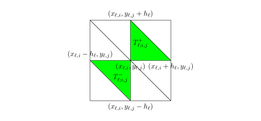
Figure 4.1: An example of element interpolation on $T^{+}_{\ell;i,j}\cup T^{-}_{\ell;i,j}$.

The following theorem describes the connection between $\Pi_{L}m$ and $m_{L}$, which gives the geometrical interpretation of $m_{L}$.

Theorem 4.1

For $m(x,y)=xy$, the following identity for the uniform interpolation $\Pi_{L}m$ in (4.7) and the commonly used approximation scheme $m_{L}$ in (4.2) holds:

$$\Pi_{L}m(x,y)=m_{L+2}(x,y),\quad(x,y)\in[-1,1]^{2}.$$ (4.8)

Proof  Let us compute $m_{L+2}(x,y)$ first. Recall the property of $\widehat{s}_{L+2}(x)$ in (3.25). Therefore, for any $x\in[x_{L+1,i},x_{L+1,i}+h_{L+1}]$ and $(x_{L+1,i},y_{L+1,j})\in\mathcal{T}^{2}_{L+1}$ we have

$$\widehat{s}_{L+2}(x)=(2x_{L+1,i}+h_{L+1})x-x_{L+1,i}(x_{L+1,i}+h_{L+1}).$$ (4.9)

Now, let us consider $(x,y)\in T^{+}_{L;i,j}$ where for any $i,j$, we have $\frac{x_{L,i}}{2}\leq\frac{x}{2}\leq\frac{x_{L,i}}{2}+h_{L+1},\frac{y_{L,j}}{2}\leq\frac{y}{2}\leq\frac{y_{L,j}}{2}+h_{L+1},\frac{x_{L,i}+y_{L,j}}{2}\leq\frac{x+y}{2}\leq\frac{x_{L,i}+y_{L,j}}{2}+h_{L+1}$. This means that we can apply (4.9) for $\frac{x}{2}$, $\frac{y}{2}$ and $\frac{x+y}{2}$, and get

$$m_{L+2}(x,y)={} 2(\widehat{s}_{L+2}(\frac{x+y}{2})-\widehat{s}_{L+2}(\frac{x}{2})-\widehat{s}_{L+2}(\frac{y}{2}))$$ (4.10)

$$={} 2\bigg{\{}\left((x_{L,i}+y_{L,j}+h_{L+1})\frac{x+y}{2}-\frac{x_{L,i}+y_{L,j}}{2}(\frac{x_{L,i}+y_{L,j}}{2}+h_{L+1})\right)$$

$$-\left((x_{L,i}+h_{L+1})\frac{x}{2}-\frac{x_{L,i}}{2}(\frac{x_{L,i}}{2}+h_{L+1})\right)$$

$$-\left((y_{L,j}+h_{L+1})\frac{y}{2}-\frac{y_{L,j}}{2}(\frac{y_{L,j}}{2}+h_{L+1})\right)\bigg{\}}$$

$$={} y_{L,j}x+x_{L,i}y-x_{L,i}y_{L,j}$$

$$={} \Pi_{L}m(x,y)$$

for any $(x,y)\in T^{+}_{L;i,j}$ and $i,j$. With the same argument, we can verify the above relation on $T^{-}_{L;i,j}$ for any $i,j$. Thus, $\Pi_{L}(xy)=m_{L+2}(x,y)$ holds for all $(x,y)\in[-1,1]^{2}$. $\square$

This theorem provides a geometrical interpretation of the commonly used approximation scheme $m_{L}(x,y)$ in (4.2), which was originally proposed from the algebraic perspective.

Now let us show the approximation property of ReLU DNN for $m(x,y)=xy$ by utilizing results we have just established. Similar to 1D, we present the next lemma for the approximation result of $\Pi_{L}m$.

Lemma 4.2

For $m(x,y)=xy$, we have

$$\|\Pi_{L}m-m\|_{L^{\infty}([-1,1]^{2})}=2^{-2(L+1)}.$$ (4.11)

Proof  For any $(x,y)\in T^{+}_{L;i,j}\cup T^{-}_{L;i,j}$, we have

$$\begin{split}|\Pi_{L}m(x,y)-m(x,y)|&=|y_{L,j}x+x_{L,i}y-x_{L,i}y_{L,j}-xy|\\ &=(x-x_{L,i})(y-y_{L,j})\\ &\leq\left(\frac{x+y-x_{L,i}-y_{L,j}}{2}\right)^{2}\\ &\leq\left(\frac{h_{L}}{2}\right)^{2}=2^{-2(L+1)}.\end{split}$$ (4.12)

Thus, we have

$$\|\Pi_{L}m-m\|_{L^{\infty}([-1,1]^{2})}=2^{-2(L+1)}.$$ (4.13)

$\square$

Based on the above connection and approximation rate of $\Pi_{L}m$, we have the next lemma.

Lemma 4.3

For multiplication function $m(x,y)=xy$ on $[-M,M]^{2}$, we have $m_{L}(x,y)\in\widehat{{\rm DNN}}_{3L}^{3}$ such that

$$\|m_{L}-m\|_{L^{\infty}([-M,M]^{2})}=M^{2}2^{-2(L-1)}.$$ (4.14)

In addition, $m_{L}(x,0)=m_{L}(0,y)=0$.

Proof  Let $\widehat{s}_{L}\in\widehat{{\rm DNN}}_{L}^{2}$ be the approximation of $s(x)=x^{2}$ as presented in Theorem 3.1. We, therefore, generalize the previous construct of $m_{L}$ as

$$m_{L}(x,y) =M^{2}\left(2\widehat{s}_{L}\left(\frac{x+y}{2M}\right)-2\widehat{s}_{L}\left(\frac{x}{2M}\right)-2\widehat{s}_{L}\left(\frac{y}{2M}\right)\right)$$ (4.15)

$$=M^{2}\Pi_{L-2}m(\frac{x}{M},\frac{y}{M})$$

for all $(x,y)\in[-M,M]^{2}$. Thus, we have $m_{L}\in\widehat{{\rm DNN}}_{3L}^{3}$ and

$$\|m_{L}-m\|_{L^{\infty}([-M,M]^{2})} =\sup_{(x,y)\in[-M,M]^{2}}\left|M^{2}\Pi_{L-2}m\left(\frac{x}{M},\frac{y}{M}\right)-M^{2}m\left(\frac{x}{M},\frac{y}{M}\right)\right|$$ (4.16)

$$=M^{2}\sup_{(x,y)\in[-1,1]^{2}}\left|\Pi_{L-2}m(x,y)-m(x,y)\right|$$

$$=M^{2}2^{-2(L-1)}.$$

$\square$

4.2 Approximation property of $\widehat{{\mathcal{N}}}_{L}^{N}$ for polynomials

Here, following our previous results for the ReLU DNN approximation of $m(x,y)=xy$ on $[-1,1]^{2}$ , we derive the super-approximation properties for polynomials by using ReLU DNN.

First, denote

$$\bm{x}^{\bm{k}}=x_{1}^{k_{1}}x_{2}^{k_{2}}\cdots x_{d}^{k_{d}}$$ (4.17)

as a monomial and $|{\bm{k}}|=\sum_{i=1}^{d}k_{i}$, which is also known as the $\ell_{1}$ norm of $\bm{k}$. To prove the approximation properties of ReLU DNN for the monomial, we need the next lemma to estimate the range of $m_{L}(x,y)$. This range will become the domain for the next hidden layer for the composition in DNN.

Lemma 4.4

If $|x|,|y|\leq M$, we have

$$|m_{L}(x,y)|=|2M^{2}(\widehat{s}_{L}(\frac{x+y}{2M})-\widehat{s}_{L}(\frac{x}{2M})-\widehat{s}_{L}(\frac{y}{2M}))|\leq M^{2}.$$ (4.18)

Proof Based on the relation in (4.15), we have

$$\sup_{(x,y)\in[-M,M]^{2}}|m_{L}(x,y)| =M^{2}\sup_{(x,y)\in[-M,M]^{2}}\left|\Pi_{L-2}m(\frac{x}{M},\frac{y}{M})\right|$$ (4.19)

$$=M^{2}\sup_{(x,y)\in[-1,1]^{2}}\left|\Pi_{L-2}m(x,y)\right|$$

$$=M^{2}.$$

$\square$

Lemma 4.5

For any monomial $M_{\bm{k}}(\bm{x})={\bm{x}}^{\bm{k}}=x_{1}^{k_{1}}x_{2}^{k_{2}}\cdots x_{d}^{k_{d}},\bm{x}\in[-1,1]^{d}$ with degree $p$, i.e., $|\bm{k}|=p$, there exists $\widehat{M}_{\bm{k}}(\bm{x})\in\widehat{{\mathcal{N}}}_{3(p-1)L}^{4}$ such that

$$\|M_{\bm{k}}(\bm{x})-\widehat{M}_{\bm{k}}(\bm{x})\|_{L^{\infty}([-1,1]^{d})}\leq(p-1)\cdot 2^{-2(L-1)}$$ (4.20)

and $\|\widehat{M}_{\bm{k}}(\bm{x})\|_{L^{\infty}([-1,1]^{d})}\leq 1$.

Proof  We establish the proof by induction for $p$. Firstly, for $p=2$ and $M_{\bm{k}}(\bm{x})=x_{i}x_{j}$, we have $\widehat{M}_{\bm{k}}(\bm{x})=m_{L}(x_{i},x_{j})\in\widehat{{\mathcal{N}}}_{3L}^{3}\subset\widehat{{\mathcal{N}}}_{3L}^{4}$ as presented in Lemma 4.3. By induction, let us prove the case with $p+1$ if $p$ holds. Then, for any $M_{\bm{k}}(\bm{x})$ with $|\bm{k}|=p+1$, we can find an $M_{\tilde{\bm{k}}}(\bm{x})$ with $\tilde{\bm{k}}=p$ and $\bm{k}=\tilde{\bm{k}}+e_{i}$ such that $M_{\tilde{\bm{k}}}(\bm{x})\in\widehat{{\mathcal{N}}}_{3(p-1)L}^{4}$ with

$$\|M_{\bm{\tilde{k}}}(\bm{x})-\widehat{M}_{\bm{\tilde{k}}}(\bm{x})\|_{L^{\infty}([-1,1]^{d})}\leq(p-1)\cdot 2^{-2(L-1)}$$ (4.21)

and $\|\widehat{M}_{\bm{\tilde{k}}}(\bm{x})\|_{L^{\infty}([-1,1]^{d})}\leq 1$. Then, we have the next construction for $\widehat{M}_{\bm{k}}(\bm{x})$:

$$\widehat{M}_{\bm{k}}(\bm{x})=m_{L}(x_{i},\widehat{M}_{\bm{\tilde{k}}}(\bm{x}))\in\widehat{{\mathcal{N}}}_{3pL}^{4}.$$ (4.22)

Then, let us check the approximation property:

$$\begin{aligned} &\|M_{\bm{k}}(\bm{x})-\widehat{M}_{\bm{k}}(\bm{x})\|_{L^{\infty}([-1,1]^{d})}\\ &\leq\|m(x_{i},M_{\bm{\tilde{k}}}(\bm{x}))-m_{L}(x_{i},\widehat{M}_{\bm{\tilde{k}}}(\bm{x}))\|_{L^{\infty}([-1,1]^{d})}\\ &\leq\|m(x_{i},M_{\bm{\tilde{k}}}(\bm{x}))-m(x_{i},\widehat{M}_{\bm{\tilde{k}}}(\bm{x}))\|_{L^{\infty}([-1,1]^{d})}+\|m(x_{i},\widehat{M}_{\bm{\tilde{k}}}(\bm{x}))-m_{L}(x_{i},\widehat{M}_{\bm{\tilde{k}}}(\bm{x}))\|_{L^{\infty}([-1,1]^{d})}\\ &\leq\|x_{i}\|_{L^{\infty}([-1,1]^{d})}\|M_{\bm{\tilde{k}}}(\bm{x})-\widehat{M}_{\bm{\tilde{k}}}(\bm{x})\|_{L^{\infty}([-1,1]^{d})}+2^{-2(L-1)}\\ &\leq(p-1)2^{-2(L-1)}+2^{-2(L-1)}\\ &\leq p2^{-2(L-1)}.\end{aligned}.$$ (4.23)

Then, following Lemma 4.4, we have $\|\widehat{M}_{\bm{k}}(\bm{x})\|_{L^{\infty}([-1,1]^{d})}\leq 1$ given the construction in (4.22) and the induction that $\|\widehat{M}_{\bm{\tilde{k}}}(\bm{x})\|_{L^{\infty}([-1,1]^{d})}\leq 1$.

$\square$

In the end, we have the next approximation result for polynomials in $\mathbb{R}^{d}$.

Lemma 4.6

For any degree-$p$ polynomial $P_{p}(\bm{x})=\sum_{|\bm{k}|\leq p}a_{\bm{k}}\bm{x}^{\bm{k}},\bm{x}\in[-1,1]^{d}$, there exists $\widehat{f}^{L}_{p}\in\widehat{{\mathcal{N}}}^{4}_{3\binom{p+d}{d}(p-1)L}$ such that

$$\|P_{p}-\widehat{f}^{L}_{p}\|_{L^{\infty}([-1,1]^{d})}\leq(p-1)\cdot 2^{-2(L-1)}\sum_{|\bm{k}|\leq p}|a_{\bm{k}}|.$$ (4.24)

Proof  This can be proven by combining Properties 2.1 and Lemma 4.5. $\square$

The above result plays a fundamental role in many studies [38, 24, 5, 26, 27, 21, 31, 30, 9, 25]. In this paper, however, we provide tighter bounds and more concise proofs for Lemmas 4.2–4.6 by applying the connection of ReLU DNNs and FEM in Theorem 4.1.

5 Representation of a 2D linear finite element function with only 2 hidden layers

In this section, we will present our unexpected discovery pertaining to the expressive power of ReLU DNNs, which derived from our investigation into ReLU DNNs in relation to hierarchical basis methods.

In terms of the approximation of ReLU DNNs for $x^{2}$, the most critical point in establishing Theorem 3.1 is that

$$(I_{\ell}-I_{\ell-1})s(x)=-h_{\ell}^{2}\sum_{i\in\mathcal{I}_{\ell}}\phi_{\ell,i}(x)=-h_{\ell}^{2}g_{\ell}(x)\in{\mathcal{N}}_{\ell}^{3}$$ (5.1)

for all $x\in\mathbb{R}$. Thus, a key question arises:

Is there composition structure for $(\Pi_{\ell}-\Pi_{\ell-1})m(x,y)$?

Thanks to Theorem 4.1, we have the following corollary for the explicit formula for $(\Pi_{\ell}-\Pi_{\ell-1})m$ on $[-1,1]^{2}$.

Corollary 5.1

For any $(x,y)\in[-1,1]^{2}$, we have

$$(\Pi_{\ell}-\Pi_{\ell-1})m(x,y)$$ (5.2)

$$=m_{\ell+2}(x,y)-m_{\ell+1}(x,y)$$

$$=2h^{2}_{\ell+1}\left(g_{\ell+1}\left(\frac{|x|}{2}\right)+g_{\ell+1}\left(\frac{|y|}{2}\right)-g_{\ell+1}\left(\frac{|x+y|}{2}\right)\right).$$

This means that $\psi_{\ell}\in\widehat{{\mathcal{N}}}_{3(\ell+2)}^{3}$ where $\psi_{\ell}=(\Pi_{\ell}-\Pi_{\ell-1})m$. Furthermore, it is worth noting that we can actually have $\psi_{\ell}\in{\mathcal{N}}_{\ell+2}^{9}$ since $g_{\ell+1}(\frac{|x+y|}{2})\in{\mathcal{N}}_{\ell+2}^{3}$.

By choosing a suitable scale, we have $\|h_{\ell}^{-2}(\Pi_{\ell}-\Pi_{\ell-1})m\|_{L^{\infty}([-1,1]^{2})}=1$. Fig. 5.1 shows function graphs of $h_{2}^{-2}(\Pi_{2}-\Pi_{1})m$ and $h_{3}^{-2}(\Pi_{3}-\Pi_{2})m$ on $[0,1]^{2}$.

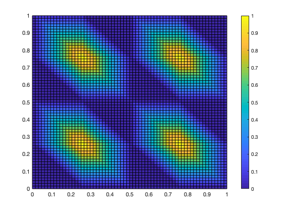
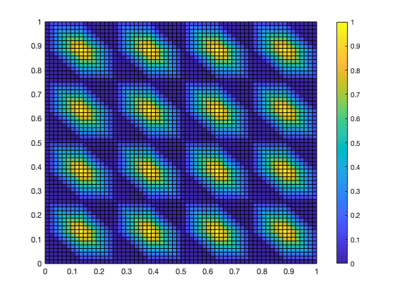
Figure 5.1: Functions of $h_{\ell}^{-2}(\Pi_{\ell}-\Pi_{\ell-1})m$ for $\ell=2$ (left) and $\ell=3$ (right) on $[0,1]^{2}$.

These graphs and meshes of $(\Pi_{\ell}-\Pi_{\ell-1})m(x,y)$ give rise to a natural discussion about the representation theorem of ReLU DNN for the basis function of the 2D linear finite element. By taking $\ell=1$ with a suitable scale, we have

$$4(\Pi_{1}-\Pi_{0})m(x,y)=\frac{1}{2}\left(g_{2}\left(\frac{x}{2}\right)+g_{2}\left(\frac{y}{2}\right)-g_{2}\left(\frac{x+y}{2}\right)\right)$$ (5.3)

for all $(x,y)\in[0,1]^{2}$. Here, $4(\Pi_{1}-\Pi_{0})m(x,y)$ equals the basis function $\varphi(x,y)$ for the linear finite element (see left-hand graph of Fig. 5.2) on the uniform mesh on $[0,1]^{2}$ with mesh size $h_{1}=\frac{1}{2}$ (see right-hand graph of Fig. 5.2).

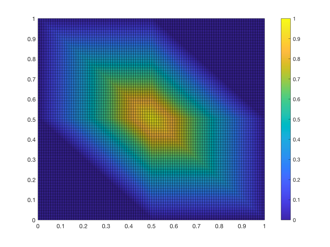
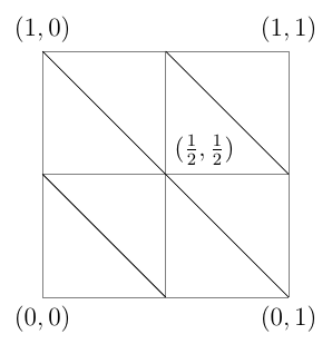
Figure 5.2: left: $\varphi(x,y)$ on $[0,1]^{2}$; right: mesh for $\ell=1$ on $[0,1]^{2}$.

Without loss of generality, we can define $\varphi(x,y)$ globally as

$$\varphi(x,y)=\begin{cases}4(\Pi_{1}-\Pi_{0})m(x,y),\quad&(x,y)\in[0,1]^{2},\\ 0,\quad&\text{others}.\end{cases}$$ (5.4)

However, this representation,

$$\varphi(x,y)=\frac{1}{2}\left(g_{2}\left(\frac{x}{2}\right)+g_{2}\left(\frac{y}{2}\right)-g_{2}\left(\frac{x+y}{2}\right)\right),$$ (5.5)

holds only for $(x,y)\in[0,1]^{2}$. Related to this observation is the simple argument that

$$\frac{1}{2}\left(g_{2}\left(\frac{x}{2}\right)+g_{2}\left(\frac{y}{2}\right)-g_{2}\left(\frac{x+y}{2}\right)\right)=\frac{1}{2}\neq 0$$ (5.6)

if $(x,y)=(\frac{3}{2},\frac{3}{2})$. On the other hand, on the assumption that the identity in (5.5) holds for all $(x,y)\in\mathbb{R}^{2}$, we can rewrite $g_{2}(x)$ as

$$g_{2}(x)=\sum_{i=0}^{4}\alpha_{i}{\rm ReLU}\left(x-\frac{i}{4}\right),$$ (5.7)

for all $x\in\mathbb{R}$ where $(\alpha_{0},\alpha_{1},\cdots,\alpha_{4})=(4,-8,8,-8,4)$ based on the relations between the linear finite element functions and ReLU DNNs on 1D [11]. This means that $g_{2}\in{\mathcal{N}}_{1}^{5}$ and $\varphi(x,y)$ can be represented by a ReLU DNN with only one hidden layer on the entire space $\mathbb{R}^{2}$. However, this representation is contradictory to the theorem in [11] that the locally supported basis function of the 2D linear finite element cannot be represented globally by ReLU DNN with just one hidden layer.

Given the global representation of $\varphi(x,y)$, [10] constructs a ReLU DNN with four hidden layers to reproduce $\varphi(x,y)$ explicitly. Although [1, 11] show that a two-hidden-layer ReLU DNN should be able to represent $\varphi(x,y)$ globally on $\mathbb{R}^{2}$, the structure of network will be extremely complicated, as well as it requires a large number of neurons. Thus, to find a concise formula to reproduce $\varphi(x,y)$ on $\mathbb{R}^{2}$ directly becomes the focus of the inquiry. Based on the discovery in (5.5) and the properties of ReLU DNNs, we can construct a ReLU DNN function with two hidden layers to represent $\varphi(x,y)$. To simplify the statement of that result, let us first denote the following ${\rm ReLU1}(x)$ function:

$${\rm ReLU1}(x):={\rm ReLU}(x)-{\rm ReLU}(x-1)\in{\mathcal{N}}_{1}^{2}.$$ (5.8)

Lemma 5.1

The basis function $\varphi(x,y)$ is in ${\mathcal{N}}_{2}^{15}$, more precisely, we have

$${\varphi}(x,y)=\frac{1}{2}\left(g_{2}\left(\frac{{\rm ReLU1}(x)}{2}\right)+g_{2}\left(\frac{{\rm ReLU1}(y)}{2}\right)-g_{2}\left(\frac{{\rm ReLU1}(x)+{\rm ReLU1}(y)}{2}\right)\right)$$ (5.9)

for all $(x,y)\in\mathbb{R}^{2}$.

Proof  According to the definition of $g_{2}(x)$ in (3.13) (or (5.7)) and ${\rm ReLU1}(x)$ in (5.8), we have $\varphi(x,y)\in{\mathcal{N}}_{2}^{15}$ and

$$\varphi(x,y)=0$$ (5.10)

for any $(x,y)\notin[0,1]^{2}$ as ${\rm ReLU1}(x)$ and ${\rm ReLU1}(y)$ will equal to $0$ or $1$. Then, (5.9) holds, given that ${\rm ReLU1}(x)=x$ and ${\rm ReLU1}(y)=y$ for $(x,y)\in[0,1]^{2}$. $\square$

By employing the above lemma, we can construct the following theorem pertaining to the representation of linear finite element functions by using ReLU DNNs with only two hidden layers on two-dimensional space.

Theorem 5.1

Assume $u_{h}$ is a two-dimensional linear finite element function, which can be written as

$$u_{h}(x,y)=\sum_{i=1}^{N}\mu_{i}\varphi(T_{i}(x,y)),$$ (5.11)

where $T_{i}:\mathbb{R}^{2}\mapsto\mathbb{R}^{2}$ is an affine mapping and $N$ denotes the number of degree of freedom. Then, $u_{h}(x)$ can be reproduced globally by a ReLU DNN with only two hidden layers and $15N$ neurons at most for each layer, i.e., $u_{h}(x,y)\in{\mathcal{N}}_{2}^{15N}$.

According to [1], any d-dimensional continuous piecewise linear function can be represented by ReLU DNNs with at most $\lceil\log_{2}(d+1)\rceil$ hidden layers. However, the representation theory in [1] requires an extremely complicated construction by induction with a tremendously high number of neurons. On the other hand, [11] shows that ReLU DNNs with only one hidden layer cannot be used to represent general linear finite element functions even on two-dimensional space. Thus, the focus inevitably turns to finding a concise and explicit representation of linear finite element functions using ReLU DNNs with only two hidden layers on two-dimensional space. Here, Theorem 5.1 provides the answer for any two-dimensional linear finite element functions on a uniform mesh or meshes, which can be obtained by adding affine mappings.

6 Concluding remarks

By carefully studying the hierarchical representation for $s(x)=x^{2}$ and $m(x,y)=xy$, we finally establish a new understanding, interpretation, and extension for the approximation results of ReLU DNNs for these two functions, which play a critically important role in a series of recent approximation results of ReLU DNNs. These discoveries provide some precise and nontrivial connections between ReLU DNNs and finite element functions especially for the hierarchical basis method. By applying these connections directly, we obtained the tightest error bound for approximating polynomials with different norms. We also showed that ReLU DNNs with this special structure can be applied only to approximate quadratic functions at an exponential rate. Furthermore, we unexpectedly developed an elegant and explicit formula whereby ReLU DNNs with two hidden layers can reproduce the basis function of the two-dimensional finite element functions on the uniform grid, which happens to be the minimal number of layers needed to represent a locally supported piecewise linear function on $\mathbb{R}^{2}$ as discussed in [11].

The connections between hierarchical basis and the ReLU DNNs open up some promising directions for the application of deeper and richer mathematical structures in finite element or other classical approximation methods in relation to ReLU DNNs. For example, it is well worth extending the explicit representation of finite element functions using ReLU DNNs on high-dimensional and unstructured meshes. A related and equally intriguing problem is that of determining how to apply ReLU DNNs in numerical solutions for partial differential equations [23] based on these connections with finite elements.

References

- [1] Raman Arora, Amitabh Basu, Poorya Mianjy, and Anirbit Mukherjee. Understanding deep neural networks with rectified linear units. In International Conference on Learning Representations, 2018.
- [2] Andrew R Barron. Universal approximation bounds for superpositions of a sigmoidal function. IEEE Transactions on Information Theory, 39(3):930–945, 1993.
- [3] Hans-Joachim Bungartz and Michael Griebel. Sparse grids. Acta numerica, 13:147–269, 2004.
- [4] George Cybenko. Approximation by superpositions of a sigmoidal function. Mathematics of Control, Signals and Systems, 2(4):303–314, 1989.
- [5] Weinan E and Qingcan Wang. Exponential convergence of the deep neural network approximation for analytic functions. Science China Mathematics, 61(10):1733–1740, 2018.
- [6] SW Ellacott. Aspects of the numerical analysis of neural networks. Acta Numerica, 3:145–202, 1994.
- [7] Ian Goodfellow, Yoshua Bengio, and Aaron Courville. Deep learning. MIT Press, 2017.
- [8] Michael Griebel. Sparse grids and related approximation schemes for higher dimensional problems. Citeseer, 2005.
- [9] Ingo Gühring, Gitta Kutyniok, and Philipp Petersen. Error bounds for approximations with deep relu neural networks in norms. Analysis and Applications, 18(05):803–859, 2020.
- [10] Juncai He. Finite Element Methods and Deep Neural Networks. PhD thesis, Peking University, 2019.
- [11] Juncai He, Lin Li, Jinchao Xu, and Chunyue Zheng. Relu deep neural networks and linear finite elements. Journal of Computational Mathematics, 38(3):502–527, 2020.
- [12] Kaiming He, Xiangyu Zhang, Shaoqing Ren, and Jian Sun. Deep residual learning for image recognition. In Proceedings of the IEEE Conference on Computer Vision and Pattern Recognition, pages 770–778, 2016.
- [13] Kaiming He, Xiangyu Zhang, Shaoqing Ren, and Jian Sun. Identity mappings in deep residual networks. In European Conference on Computer Vision, pages 630–645. Springer, 2016.
- [14] Kurt Hornik, Maxwell Stinchcombe, and Halbert White. Multilayer feedforward networks are universal approximators. Neural Networks, 2(5):359–366, 1989.
- [15] Gao Huang, Zhuang Liu, Laurens Van Der Maaten, and Kilian Q Weinberger. Densely connected convolutional networks. In CVPR, volume 1, page 3, 2017.
- [16] Lee K Jones. A simple lemma on greedy approximation in hilbert space and convergence rates for projection pursuit regression and neural network training. The Annals of Statistics, pages 608–613, 1992.
- [17] Jason M Klusowski and Andrew R Barron. Approximation by combinations of relu and squared relu ridge functions with and controls. IEEE Transactions on Information Theory, 64(12):7649–7656, 2018.
- [18] Alex Krizhevsky, Ilya Sutskever, and Geoffrey E. Hinton. Imagenet classification with deep convolutional neural networks. In International Conference on Neural Information Processing Systems, pages 1097–1105, 2012.
- [19] Yann LeCun, Yoshua Bengio, and Geoffrey Hinton. Deep learning. Nature, 521(7553):436, 2015.
- [20] Moshe Leshno, Vladimir Ya Lin, Allan Pinkus, and Shimon Schocken. Multilayer feedforward networks with a nonpolynomial activation function can approximate any function. Neural Networks, 6(6):861–867, 1993.
- [21] Jianfeng Lu, Zuowei Shen, Haizhao Yang, and Shijun Zhang. Deep network approximation for smooth functions. arXiv preprint arXiv:2001.03040, 2020.
- [22] Lu Lu, Pengzhan Jin, Guofei Pang, Zhongqiang Zhang, and George Em Karniadakis. Learning nonlinear operators via deeponet based on the universal approximation theorem of operators. Nature Machine Intelligence, 3(3):218–229, 2021.
- [23] Lu Lu, Xuhui Meng, Zhiping Mao, and George Em Karniadakis. Deepxde: A deep learning library for solving differential equations. SIAM Review, 63(1):208–228, 2021.
- [24] Zhou Lu, Hongming Pu, Feicheng Wang, Zhiqiang Hu, and Liwei Wang. The expressive power of neural networks: A view from the width. In Advances in Neural Information Processing Systems, pages 6231–6239, 2017.
- [25] Carlo Marcati, Joost AA Opschoor, Philipp C Petersen, and Christoph Schwab. Exponential relu neural network approximation rates for point and edge singularities. arXiv preprint arXiv:2010.12217, 2020.
- [26] Hadrien Montanelli and Qiang Du. New error bounds for deep relu networks using sparse grids. SIAM Journal on Mathematics of Data Science, 1(1):78–92, 2019.
- [27] Hadrien Montanelli, Haizhao Yang, and Qiang Du. Deep relu networks overcome the curse of dimensionality for bandlimited functions. arXiv preprint arXiv:1903.00735, 2019.
- [28] Guido F Montufar, Razvan Pascanu, Kyunghyun Cho, and Yoshua Bengio. On the number of linear regions of deep neural networks. In Advances in Neural Information Processing Systems, pages 2924–2932, 2014.
- [29] Vinod Nair and Geoffrey E Hinton. Rectified linear units improve restricted boltzmann machines. In Proceedings of the 27th International Conference on Machine Learning, pages 807–814, 2010.
- [30] Joost AA Opschoor, Philipp C Petersen, and Christoph Schwab. Deep relu networks and high-order finite element methods. Analysis and Applications, pages 1–56, 2020.
- [31] Joost AA Opschoor, Christoph Schwab, and Jakob Zech. Exponential relu dnn expression of holomorphic maps in high dimension. SAM Research Report, 2019, 2019.
- [32] Allan Pinkus. Approximation theory of the mlp model in neural networks. Acta Numerica, 8:143–195, 1999.
- [33] Tomaso Poggio, Hrushikesh Mhaskar, Lorenzo Rosasco, Brando Miranda, and Qianli Liao. Why and when can deep-but not shallow-networks avoid the curse of dimensionality: a review. International Journal of Automation and Computing, 14(5):503–519, 2017.
- [34] Jonathan W Siegel and Jinchao Xu. Approximation rates for neural networks with general activation functions. Neural Networks, 128:313–321, 2020.
- [35] Jonathan W Siegel and Jinchao Xu. High-order approximation rates for neural networks with activation functions. arXiv preprint arXiv:2012.07205, 2020.
- [36] Matus Telgarsky. Benefits of depth in neural networks. Journal of Machine Learning Research, 49(June):1517–1539, 2016.
- [37] Jinchao Xu. Finite neuron method and convergence analysis. Communications in Computational Physics, 28(5):1707–1745, 2020.
- [38] Dmitry Yarotsky. Error bounds for approximations with deep relu networks. Neural Networks, 94:103–114, 2017.