AdS/BCFT correspondence and BTZ black hole thermodynamics within Horndeski gravity

Abstract

In this work, we study gravity duals of conformal field theories with boundaries$-$known as AdS/BCFT correspondence, put forward by Takayanagi Takayanagi:2011zk $-$within a scalar-tensor theory, as proposed by Horndeski in 4D Horndeski . We consider the case of 3D gravity dual to 2D BCFT, take a Gibbons-Hawking surface term modified by Horndeski’s theory and find the corresponding 3D (Bañados-Teitelboim-Zanelli) black hole solutions. We analyze the effects of Horndeski gravity on the profile of the extra boundary for the black hole by using an approximate analytic solution. Performing a holographic renormalization, we calculate the free energy and obtain the total entropy and corresponding area, as well as the boundary entropy for the black hole. In particular, the boundary entropy found here can be seen as an extension of the one proposed by Takayanagi. From the free energy, we perform a systematic study of the 3D black hole thermodynamics and present, among our results, an indication of the restoration of conformal symmetry for high temperatures. Finally, we present a study on the influence of the Horndeski gravity on the Hawking-Page phase transition where we can see the stable and unstable phases throughout the plane of free energy versus temperature.

I Introduction

Einstein’s gravity is supported by both strong theoretical and experimental evidences. The observation of gravitational waves from a binary black hole merger, as reported in Ref. Abbott:2016blz , was expected as one of the crucial tests for general relativity (GR). Despite this huge success, the last three decades brought some questions that could not be answered by GR. These questions are related to both theoretical aspects and observational results. The very interesting review in Ref. Capozziello:2011et pointed out basically two classes of “shortcomings in GR” on the UV and IR scales. In the UV region one has the quantum gravity problem, and in the IR regime, the dark energy and dark matter issues. In order to address these questions new approaches were proposed known as extended theories of gravity. Such theories start with the inclusion of higher-order terms in curvature invariants in the effective Lagrangian such as, for instance, $R^{2}$ and $R^{\alpha\beta\gamma\delta}R_{\alpha\beta\gamma\delta}$ Gottlober:1989ww ; Adams:1990pn ; Amendola:1993bg , or through minimal or nonminimal coupling of scalar fields with the geometry such as, for example, $\phi^{2}R$ Maeda:1988ab ; Wands:1993uu ; Capozziello:1998dq . The approach that takes into account a single scalar field in general relativity is known as Horndeski gravity Horndeski ; Charmousis:2011bf ; Charmousis:2011ea ; Starobinsky:2016kua ; Bruneton:2012zk ; Cisterna:2014nua ; Maselli:2016gxk ; Heisenberg:2018vsk ; Hajian:2020dcq . This model is quite interesting because it is the most general scalar-tensor theory with second-order field equations in four dimensions.

Besides Horndeski gravity, in this work we consider two other essential components. The first one is related to the AdS/CFT correspondence or duality, whose fundamental concepts were explained in Refs. Maldacena:1997re ; Gubser:1998bc ; Witten:1998qj ; Aharony:1999ti . Over the past two decades since its emergence, many investigations around AdS/CFT have provided great insights on the study of strong coupled systems. Among many interesting features of this correspondence, one should note the possibility of building models on the gravity side that are duals to phases of a nonconformal plasma at finite temperature or density. It is worthwhile to mention that in the recent Refs. Jiang:2017imk ; Baggioli:2017ojd ; Liu:2018hzo ; Li:2018kqp ; Li:2018rgn ; Wang:2019jyw , the authors presented some applications of AdS/CFT in the Horndeski scenario.

The inclusion of another boundary in the original AdS/CFT duality leads to the AdS/BCFT correspondence, which has attracted a lot of attention in the last years. This proposal was presented by Takayanagi Takayanagi:2011zk and soon after by Fujita, Takayanagi and Tonni Fujita:2011fp as an extension of the standard AdS/CFT correspondence.

The main point in AdS/CFT is based on the fact that the AdS_d+1 space is dual to a conformal field in $d$ dimensions. In this case the AdS_d+1 symmetry, which is $SO(2,d)$, is the same as the conformal symmetry of the CFT_d. However when one adds a new boundary with $d-1$ dimensions to the CFT_d, one notices the breaking of $SO(2,d)$ into a $SO(2,d-1)$ group. In this sense, due to the insertion of this new boundary, this theory is known as boundary conformal field theory (BCFT) and then one can construct a correspondence called AdS/BCFT Takayanagi:2011zk ; Fujita:2011fp ; Nozaki:2012qd ; Fujita:2012fp ; Melnikov:2012tb ; Magan:2014dwa ; Erdmenger:2014xya ; Erdmenger:2015spo ; Flory:2017ftd . In particular, in this work we deal with an AdS₃/BCFT₂ correspondence.

As we know, in the standard AdS/CFT correspondence we have an asymptotically anti–de Sitter (AdS) spacetime N, which has a boundary M with a Dirichlet boundary condition on it. On the other hand, following the AdS/BCFT prescription, we introduce an additional boundary Q wrapping N, whose interception with M is the manifold P, as shown in Fig. 1. On the hypersurface Q, the bulk-metric of N should satisfy a Neumann boundary condition. Also by looking at Fig. 1 one should notice that the $d$-dimensional spacetime M is bounded by P, which will also bound Q. Within this construction, the $d+1$-dimensional spacetime N is limited by a region defined by $M\cup Q$.

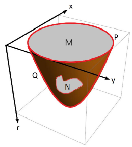
Figure 1: Holographic description of BCFT, where we have the asymptotically AdS bulk spacetime N with conformal boundary M and additional boundary Q. Here P is the intersection of M and Q.

The second essential component of this work is to deal with a finite-temperature theory within the AdS/CFT correspondence. Following the standard procedure we include a black hole in the bulk geometry and interpret the Hawking temperature as the temperature of the CFT side.

In the past, $(2+1)$-dimensional gravity was considered as a toy model since (as pointed out in Ref. Carlip:1995qv ) it does not have a Newtonian limit nor any propagating degrees of freedom. However, after the work of Bañados, Teitelboim, and Zanelli (BTZ) Banados:1992wn ; Banados:1992gq , it was realized that such a kind of (2+1) theory has a solution, known as the BTZ black hole, with some interesting features: an event horizon (and in some cases an additional inner horizon, if one includes rotations) presenting thermodynamic properties somehow similar to the black holes in (3+1) dimensions and being asymptotically anti-de Sitter. For our purposes in this paper we choose to work with a planar BTZ black hole with a nontrivial axis profile.

II Methodological route and achievements

Motivated by the recent application of the AdS/CFT duality in Horndeski gravity together with the emergence of AdS/BCFT and taking into account the importance of (2+1)$-$dimensional black holes, in this work we establish the AdS/BCFT correspondence in Horndeski gravity and study the thermodynamics of the corresponding AdS-BTZ black hole. Here we present a summary of the main results achieved in this work:

• First, we study the influence of the Horndeski parameters on the BCFT theory. Apart from a complete numerical solution, we derive an approximate analytical solution that is useful for determining the role of Q profile and perform an analysis of all quantities in this work;

• We construct a holographic renormalization for this setup and compute the free energy for both the AdS-BTZ black hole and thermal AdS;

• From the free energy, we compute the total and boundary entropies. In the case of the boundary entropy, one can see it as an extension of the results found in Refs. Takayanagi:2011zk ; Fujita:2011fp ;

• Assuming that the total entropy and total area of the AdS-BTZ black hole are related by the Bekenstein-Hawking formula, we see that the influence of Horndeski gravity enables an increase of the black hole area as we increase the absolute value of the Horndeski parameter. This feature of our model is not present in the usual BCFT theory as discussed, for instance, in Refs. Takayanagi:2011zk ; Fujita:2011fp ; Magan:2014dwa .

• At zero temperature, our setup exhibits a nonzero or residual boundary entropy, at least in certain conditions which depend on the tension of the Q profile. Besides, zero entropy seems to imply a minimum nonzero temperature.

• From the free energy we also compute the thermodynamic observables, including the heat capacity, sound speed and trace anomaly and plot their behavior against the temperature. In particular, the trace anomaly goes to zero at high temperatures indicating a restoration of the conformal symmetry or a nontrivial BCFT.

• We study the Hawking-Page phase transition (HPPT) in this setup. The presence of the Horndeski term allow us to analyze this transition of the free energy as a function of the temperature, as in other higher-dimensional theories. This differs from the results presented in Refs. Takayanagi:2011zk ; Fujita:2011fp , where the authors plotted the free energy as a function of the tension of the Q profile.

This work is organized as follows. In Section III, we present our gravitational setup and how to combine it with BCFT theory. In the Section IV, we consider a BTZ black hole in Horndeski gravity and study the influence of the Horndeski parameter on Q profile. In Section V, by performing a holographic renormalization we compute the Euclidean on-shell actions associated with the BTZ and thermal AdS space. In Section VI, from the euclidean on-shell action, we derive the BTZ black hole entropy, and in Section VII, we present a systematic study of its thermodynamic quantities. In section VIII, we present the Hawking-Page phase transition between the BTZ black hole and thermal AdS space. Finally, in Section IX we present our conclusion and final comments.

III The Setup

III.1 Horndeski’s Lagrangian

In this section, we present the outline of Horndeski gravity. The complete Horndeski Lagrangian density can be written in a general form as:

$${\cal L}_{H}={\cal L}_{EH}+{\cal L}_{2}+{\cal L}_{3}+{\cal L}_{4}+{\cal L}_{5}\,,$$ (1)

where ${\cal L}_{EH}=\kappa(R-2\Lambda)$ is the Einstein-Hilbert Lagrangian density, $R$ is the Ricci scalar, $\Lambda$ the cosmological constant, $\kappa=(16\pi G_{N})^{-1}$, $G_{N}$ is Newton’s gravitational constant, and we choose $4\pi G_{N}=1$, so that $\kappa=1/4$. The Lagragians ${\cal L}_{2}$, ${\cal L}_{3}$, ${\cal L}_{4}$ and ${\cal L}_{5}$ are given by:

$${\cal L}_{2} = G_{2}(X,\phi)\,,$$

$${\cal L}_{3} = -G_{3}(X,\phi)\Box\phi\,,$$

$${\cal L}_{4} = -G_{4}(X,\phi)R+\partial_{X}G_{4}(X,\phi)\delta^{\mu\nu}_{\alpha\beta}\nabla^{\alpha}_{\mu}\phi\nabla^{\beta}_{\nu}\phi\,,$$

$${\cal L}_{5} = -G_{5}(X,\phi)G_{\mu\nu}\nabla^{\mu}\nabla^{\nu}\phi-\frac{1}{6}\partial_{X}G_{5}(X,\phi)\delta^{\mu\nu\rho}_{\alpha\beta\gamma}\nabla^{\alpha}_{\mu}\phi\nabla^{\beta}_{\nu}\phi\nabla^{\gamma}_{\rho}\phi\,,$$ (2)

with $G_{2}$, $G_{3}$, $G_{4}$, and $G_{5}$ being arbitrary functions of the scalar field $\phi$ and $X$ is defined by $X\equiv-\frac{1}{2}\nabla_{\mu}\phi\nabla^{\mu}\phi$, while $G_{\mu\nu}=R_{\mu\nu}-\frac{1}{2}g_{\mu\nu}R$ is the Einstein tensor, and $g_{\mu\nu}$ is the spacetime metric. For a detailed review of Honderski gravity, one can see Ref. Kobayashi:2019hrl .

In particular, we are interested in a special subclass of Horndeski gravity that has a nonminimal coupling between the standard scalar term and the Einstein tensor Charmousis:2011bf ; Charmousis:2011ea ; Starobinsky:2016kua ; Bruneton:2012zk ; Brito:2019ose ; Santos:2020xox . In this sense, Eq. (1) becomes:

$${\cal L}_{H}\equiv{\cal L}_{EH}+{\cal L}_{2} = (R-2\Lambda)-\frac{1}{2}(\alpha g_{\mu\nu}-\gamma\,G_{\mu\nu})\nabla^{\mu}\phi\nabla^{\nu}\phi\,,$$ (3)

where $\alpha$ and $\gamma$ are the usual Horndeski parameters, which control the strength of the kinetic couplings, and have mass dimensions 0 and $-2$, respectively. For convenience, we introduce the dimensionless parameter $\gamma^{\prime}=-\gamma\Lambda$. Note that the Lagrangian density in Eq. (3), is invariant under displacement symmetry ($\phi\to\phi\,+\,constant$) and parity transformation ($\phi\to-\phi$).

III.2 AdS₃/BCFT₂ correspondence with Horndeski $\gamma^{\prime}$ dependence

In this section, we discuss the AdS/BCFT correspondence within Horndeski gravity. As discussed in Refs. Takayanagi:2011zk ; Fujita:2011fp , for the construction of boundary systems we need to take into account a Gibbons-Hawking surface term. In addition, such a surface term for Horndeski $\gamma^{\prime}$-dependent gravity was proposed in Ref. Li:2018rgn . Motivated by these works, we propose the total action including the contributions coming from the surfaces N, Q and P, besides matter terms from N and Q and the counterterms from P:

$$S = S^{N}+S^{N}_{mat}+S^{Q}+S^{Q}_{mat}+S^{P}_{ct}\,,$$ (4)

where $S^{N}_{mat}$ describes ordinary matter that is supposed to be a perfect fluid, and

$$S^{N}=\kappa\int_{N}{d^{3}x\sqrt{-g}\mathcal{L}_{H}}$$ (5)

$$S^{Q}=2\kappa\int_{bdry}{d^{2}x\sqrt{-h}\mathcal{L}_{bdry}}$$ (6)

$$S^{Q}_{mat}=2\int_{Q}{d^{2}x\sqrt{-h}\mathcal{L}_{mat}}$$ (7)

$$S^{P}_{ct}=2\kappa\int_{ct}{d^{2}x\sqrt{-h}\mathcal{L}_{ct}}\,,$$ (8)

where $\mathcal{L}_{H}$ was defined in Eq. (3) and

$$\mathcal{L}_{bdry} = (K-\Sigma)+\frac{\gamma^{\prime}}{4\Lambda}(\nabla_{\mu}\phi\nabla_{\nu}\phi n^{\mu}n^{\nu}-(\nabla\phi)^{2})K+\frac{\gamma^{\prime}}{4\Lambda}\nabla_{\mu}\phi\nabla_{\nu}\phi K^{\mu\nu}\,,$$ (9)

$$\mathcal{L}_{ct} = c_{0}+c_{1}R+c_{2}R^{ij}R_{ij}+c_{3}R^{2}+b_{1}(\partial_{i}\phi\partial^{i}\phi)^{2}+...$$ (10)

Note that $\mathcal{L}_{mat}$ is a Lagrangian of possible matter fields on Q and $\mathcal{L}_{bdry}$ corresponds to the Gibbons-Hawking $\gamma^{\prime}$-dependent terms associated with the Horndeski gravity. In the boundary Lagrangian, Eq. (9), $K_{\mu\nu}=h^{\beta}_{\mu}\nabla_{\beta}n_{\nu}$ is the extrinsic curvature, $h_{\mu\nu}$ is the induced metric and $n^{\mu}$ is the normal vector of the hypersurface Q. The traceless contraction of $K_{\mu\nu}$ is $K=h^{\mu\nu}K_{\mu\nu}$, and $\Sigma$ is the boundary tension on Q. Furthermore, ${\cal L}_{ct}$ are boundary counterterms localized on P which is required to be an asymptotic AdS spacetime. By imposing a Neumann boundary condition in Eq. (9), we obtain

$$K_{\alpha\beta}-h_{\alpha\beta}(K-\Sigma)+\frac{\gamma^{\prime}}{4\Lambda}H_{\alpha\beta}=\kappa{\cal S}^{Q}_{\alpha\beta}\,,$$ (11)

where we defined

$$H_{\alpha\beta}\equiv(\nabla_{\alpha}\phi\nabla_{\beta}\phi n^{\alpha}n^{\beta}-(\nabla\phi)^{2})(K_{\alpha\beta}-h_{\alpha\beta}K)-(\nabla_{\alpha}\phi\nabla_{\beta}\phi)h_{\alpha\beta}K\,,$$ (12)

$${\cal S}^{Q}_{\alpha\beta}=-\frac{2}{\sqrt{-h}}\frac{\delta S^{Q}_{mat}}{\delta h^{\alpha\beta}}\,.$$ (13)

Considering $S^{Q}_{mat}$ as a constant one has ${\cal S}^{Q}_{\alpha\beta}=0$. Then, we can write

$$K_{\alpha\beta}-h_{\alpha\beta}(K-\Sigma)+\frac{\gamma^{\prime}}{4\Lambda}H_{\alpha\beta}=0\,.$$ (14)

On the gravitational side, for Einstein-Horndeski gravity assuming that $S^{N}_{mat}$ is constant, and varying $S^{N}$ with respect to $g_{\alpha\beta}$ and $\phi$, and $S^{Q}$ with respect to $\phi$, respectively, we have:

$${\cal E}_{\alpha\beta}[g_{\mu\nu},\phi]=-\frac{2}{\sqrt{-g}}\frac{\delta S^{N}}{\delta g^{\alpha\beta}}\,,\quad{\cal E}_{\phi}[g_{\mu\nu},\phi]=-\frac{2}{\sqrt{-g}}\frac{\delta S^{N}}{\delta\phi}\,,\quad{\cal F}_{\phi}[g_{\mu\nu},\phi]=-\frac{2}{\sqrt{-h}}\frac{\delta S^{Q}}{\delta\phi}\,.$$

Then, one finds:

$${\cal E}_{\mu\nu}[g_{\mu\nu},\phi] = G_{\mu\nu}+\Lambda g_{\mu\nu}-\frac{\alpha}{2}\left(\nabla_{\mu}\phi\nabla_{\nu}\phi-\frac{1}{2}g_{\mu\nu}\nabla_{\lambda}\phi\nabla^{\lambda}\phi\right)$$ (16)

$$- \frac{\gamma^{\prime}}{2\Lambda}\left(\frac{1}{2}\nabla_{\mu}\phi\nabla_{\nu}\phi R-2\nabla_{\lambda}\phi\nabla_{(\mu}\phi R^{\lambda}_{\nu)}-\nabla^{\lambda}\phi\nabla^{\rho}\phi R_{\mu\lambda\nu\rho}\right)$$

$$- \frac{\gamma^{\prime}}{2\Lambda}\left(-(\nabla_{\mu}\nabla^{\lambda}\phi)(\nabla_{\nu}\nabla_{\lambda}\phi)+(\nabla_{\mu}\nabla_{\nu}\phi)\Box\phi+\frac{1}{2}G_{\mu\nu}(\nabla\phi)^{2}\right)$$

$$+ \frac{\gamma^{\prime}g_{\mu\nu}}{2\Lambda}\left(-\frac{1}{2}(\nabla^{\lambda}\nabla^{\rho}\phi)(\nabla_{\lambda}\nabla_{\rho}\phi)+\frac{1}{2}(\Box\phi)^{2}-(\nabla_{\lambda}\phi\nabla_{\rho}\phi)R^{\lambda\rho}\right),$$

$${\cal E}_{\phi}[g_{\mu\nu},\phi] = \nabla_{\mu}\left[\left(\alpha g^{\mu\nu}+\frac{\gamma^{\prime}}{\Lambda}G^{\mu\nu}\right)\nabla_{\nu}\phi\right]\,,$$ (17)

$${\cal F}_{\phi}[g_{\mu\nu},\phi] = \frac{\gamma^{\prime}}{4\Lambda}(\nabla_{\mu}\nabla_{\nu}\phi n^{\mu}n^{\nu}-(\nabla^{2}\phi))K+\frac{\gamma^{\prime}}{4\Lambda}(\nabla_{\mu}\nabla_{\nu}\phi)K^{\mu\nu}\,.$$ (18)

Note that, from the Euler-Lagrange equation, ${\cal E}_{\phi}[g_{\mu\nu},\phi]={\cal F}_{\phi}[g_{\mu\nu},\phi]$.

IV Q-profile within A BTZ black hole in Horndeski gravity

In this section, we describe our BTZ black hole and construct the profile of the hypersurface Q taking into account the influence of Horndeski gravity.

The three-dimensional metric of the BTZ black hole is defined as the three-dimensional metric as Banados:1992wn ; Banados:1992gq :

$$ds^{2}=\frac{{{L}}^{2}}{r^{2}}\left(-{f}(r)d{{t}}^{2}+d{y}^{2}+\frac{dr^{2}}{{f}(r)}\right)\,.$$ (19)

A condition that deals with static configurations of black holes, which can be spherically symmetric for certain Galileons, was presented in Ref. Bravo-Gaete:2013dca to discuss the no-hair theorem. The no-hair theorem requires that the square of radial component of the conserved current vanishes identically without restricting the radial dependence of the scalar field, which implies:

$$\alpha g_{rr}-\gamma G_{rr}=0\,,$$ (20)

or, equivalently

$$\alpha g_{rr}+\frac{\gamma^{\prime}}{\Lambda}G_{rr}=0\,.$$

From this condition we have ${\cal E}_{\phi}[g_{rr},\phi]=0$. These solutions can be asymptotically dS or AdS for $\alpha/\gamma<0$ or $\alpha/\gamma>0$, respectively, as discussed in Refs. Anabalon:2013oea ; Santos:2020xox . From now on, we will work with the asymptotically AdS case in three dimensions such that ${\Lambda}=-3/{L}^{2}$, where $L$ is the AdS radius. Then, since $\Lambda<0$, the parameters $\gamma$ and $\gamma^{\prime}=-\gamma\Lambda$ have the same sign.

Thus, we consider just $\phi=\phi(r)$ and define $\phi{{}^{\prime}}(r)\equiv{\psi}(r)$. It can be shown that the equations ${\cal E}_{\phi}[g_{rr},\phi]={\cal E}_{rr}[g_{rr},\phi]=0$ are satisfied and will be used to calculate the horizon function ${f}(r)$ and $\psi(r)$, so that:

$${f}(r) = \frac{\alpha}{\gamma^{\prime}}-\left(\frac{r}{{r}_{h}}\right)^{2},$$ (21)

$${\psi}^{2}(r) = -\frac{6(\alpha-\gamma^{\prime})}{\alpha\gamma^{\prime}r^{2}{f}(r)}.$$ (22)

Performing the transformations Brito:2019ose :

$${f}(r)\to\frac{\alpha}{\gamma^{\prime}}\,{f}(r),\,\, {r}_{h}^{2}\to\frac{\gamma^{\prime}}{\alpha}\,{r}_{h}^{2}$$ (23)

$${L}\to\sqrt{\frac{\alpha}{\gamma^{\prime}}}\,L\,, {t}\to\frac{\gamma^{\prime}}{\alpha}\,t$$ (24)

$${y} \to \sqrt{\frac{\gamma^{\prime}}{\alpha}}\,y$$ (25)

in the above equations, one finds that the metric (19) is invariant, while the horizon function $f(r)$ and $\psi(r)$ read

$$f(r) = 1-\left(\frac{r}{r_{h}}\right)^{2},$$ (26)

$${\psi}^{2}(r) = -\frac{6(\alpha-\gamma^{\prime})}{\alpha^{2}r^{2}{f}(r)}\,.$$ (27)

The scalar field given by Eq. (27) should be real, and since $f(r)\geq 0$, we impose the constraint

$${\alpha}\leq{\gamma^{\prime}}\,,$$ (28)

with three possibilities:

• $\alpha=\gamma^{\prime}$;

• $\alpha>0$ and $\gamma^{\prime}>0$;

• $\alpha<0$ and $\gamma^{\prime}<0$.

The first choice implies $\psi(r)=\phi^{\prime}(r)=0$. The second gives $\alpha/\gamma^{\prime}<1$, while the third is satisfied for $\alpha/\gamma^{\prime}>1$. The physical consequences of these choices will be associated with the solutions of three-dimensional Horndeski gravity to be discussed below.

The Hawking temperature implied by the metric (19), is given by

$$T_{H}=\dfrac{1}{4\pi}|f^{\prime}(r_{h})|=\frac{1}{2\pi r_{h}}\,,$$ (29)

which is equal to the temperature of the dual BCFT theory $T_{BCFT}=T_{H}$.

Now, in order to construct the Q boundary profile, one has that the induced metric on this surface given by

$$ds^{2}_{\rm ind}=\frac{L^{2}}{r^{2}}\left(-f(r)dt^{2}+\frac{g^{2}(r)dr^{2}}{f(r)}\right)\,,$$ (30)

where $g^{2}(r)=1+{y^{\prime}}^{2}(r)f(r)$ with $y{{}^{\prime}}(r)=dy/dr$. Then, the normal vectors on Q can be represented by

$$n^{\mu}=\frac{r}{Lg(r)}\,\left(0,\,1,\,-{f(r)y{{}^{\prime}}(r)}\right)\,.$$ (31)

Fulfilling the no-hair theorem, meaning ${\cal F}_{\phi}[h_{rr},\phi]=0$, one can solve the Eq. (14), so that

$$y{{}^{\prime}}(r) = \frac{(\Sigma L)}{\sqrt{1-\dfrac{\gamma^{\prime}\psi^{2}(r)}{4\Lambda}-(\Sigma L)^{2}\left(1-\left(\dfrac{r}{r_{h}}\right)^{2}\right)}}\,,$$ (32)

with $\psi(r)$ given by Eq. (27), so that:

$$y{{}^{\prime}}(r) = \frac{(\Sigma L)}{\sqrt{1-\dfrac{\xi^{\prime}}{r^{2}\Lambda\left(1-\left(\dfrac{r}{r_{h}}\right)^{2}\right)}-(\Sigma L)^{2}\left(1-\left(\dfrac{r}{r_{h}}\right)^{2}\right)}}\,,$$ (33)

where $\xi^{\prime}$ is defined as

$$\xi^{\prime}=-\frac{3}{2}\frac{\gamma^{\prime}}{\alpha}\left(1-\frac{\gamma^{\prime}}{\alpha}\right)\,.$$ (34)

If we choose $\alpha=\gamma^{\prime}$, then $\xi^{\prime}=0$. The second possibility is to take $\gamma^{\prime}/\alpha>1$, so that the parameter $\xi^{\prime}$ is positive and can be large. Third, for $\gamma^{\prime}/\alpha<1$, $\xi^{\prime}$ is negative and small. From now on, we consider this third case, except when explicitly mentioned. Besides, we can introduce $\Sigma L=\cos(\theta{{}^{\prime}})$ where $\theta{{}^{\prime}}$ is the angle between the positive direction of the $y$ axis and the hypersurface Q.

The equation for $y{{}^{\prime}}(r)$ can be solved numerically, and we can obtain the Q-profile for the $\gamma$-dependent Horndeski terms (for $\xi^{\prime}=0$ and $\xi^{\prime}<0$) as shown in the left panel of Fig. 2. Beyond the numerical solutions, we can analyze some particular cases regarding the study of the UV and IR regimes. Thus, for the UV case, by performing an expansion at $r\to 0$ the Eq. (33) becomes

$$y_{{}_{UV}}(r)=y_{0}+\frac{r\cos(\theta{{}^{\prime}})}{\sqrt{-\xi^{\prime}}}.$$ (35)

In the above equation, considering for instance $\theta^{\prime}=\pi/2$ or $3\pi/2$, we have

$$y_{{}_{UV}}(r)=y_{0}={\rm constant}.$$ (36)

This corresponds to a zero-tension limit $\Sigma\to 0$.

Now, for the IR case, we take $r\to\infty$, so that Eq. (22) implies $\psi(r\to\infty)=0$, and then $\phi=$ constant, which ensures a genuine vacuum solution. Plugging this result into Eq. (33), in the limit $r\to\infty$, we have

$$y_{{}_{IR}}(r)=y_{0}+\ln(r/r_{h}).$$ (37)

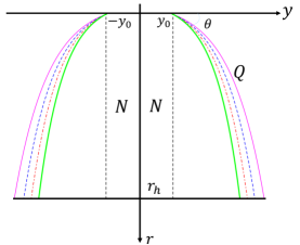
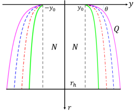
Figure 2: Q boundary profile for the BTZ black hole within Horndeski gravity considering the values for $\theta^{\prime}=2\pi/3$, $\theta=\pi-\theta^{\prime}$, $\alpha=-8/3$ with $\gamma^{\prime}=0$ (solid), $\gamma^{\prime}=-0.1$ (dashed), $\gamma^{\prime}=-0.2$ (dot dashed), and $\gamma^{\prime}=-0.3$ (thick). The dashed parallel vertical lines represent the UV solution, Eq. (36). The region between the negative and positive branches of curves Q represent the bulk N. Left panel: we show the complete numerical solution for the Eq. (33). Right panel: we show the approximated solution for small values of $\xi^{\prime}$, from the Eq. (39).

Another approximate analytical solution for $y(r)$ can be obtained by performing an expansion for very small $\xi^{\prime}$ in Eq. (33). Considering this expansion up to first order in $\xi^{\prime}$, we obtain

$$y_{{}_{Q}}\equiv y(r) = y_{0}+r_{h}\sinh^{-1}\left[\frac{r}{r_{h}}\cot(\theta{{}^{\prime}})\right]+\frac{\xi^{\prime}L^{2}\cos(\theta{{}^{\prime}})}{r_{h}}\tan^{-1}\left[\frac{r}{r_{h}\sqrt{1-\cos^{2}(\theta{{}^{\prime}})f(r)}}\right]$$ (38)

$$+ \xi^{\prime}L^{2}\cos(\theta{{}^{\prime}})\frac{\sqrt{1-\cos^{2}(\theta{{}^{\prime}})f(r)}}{{r(-1+\cos^{2}(\theta{{}^{\prime}}))^{2}}}\left[{1+\frac{r^{2}\cos^{4}(\theta{{}^{\prime}})}{r^{2}_{h}-r^{2}_{h}\cos^{2}(\theta{{}^{\prime}})f(r)}}\right]+\mathcal{O}(\xi^{\prime 2})\,.$$ (39)

It is worthwhile to mention that we consider $r_{h}^{2}\gg\xi^{\prime}L^{2}$, where $L$ is large to satisfy the AdS/CFT correspondence. In the right panel of Fig. 2, we plot the $y_{{}_{Q}}=y(r)$ profile from Eq. (39), which represents our holographic description of BCFT within Horndeski’s theory. Note that the bulk spacetime N is asymptotically AdS with two boundaries M and Q. The interception of M and Q is represented by P in Fig. 1. It is worthwhile to mention that the Q profile is obtained from the solution $y_{{}_{Q}}=y(r)$.

Note that the UV solution $y_{{}_{UV}}(r)=$ constant, Eq. (36) is similar to a lower-dimensional Randall-Sundrum (RS) brane, which is perpendicular to the boundary M. These RS-like branes could be represented in Fig 2 by the dashed parallel vertical lines. Further, as one increases the Horndeski parameter $\gamma^{\prime}$, one can see that the surface Q gets closer to the RS-like branes.

V Holographic renormalization

In this section we present the holographic renormalization scheme in order to compute the Euclidean on-shell action which is related to the free energy of the corresponding thermodynamic system. The holographic renormalization, as it is called within the AdS/CFT program, is a steady approach to remove divergences from infinite quantities on the gravitational side of the correspondence Henningson:1998gx ; deBoer:1999tgo . Such a renormalization on the gravity side will work similarly to the usual renormalization of the gauge field theory on the boundary.

Our holographic scheme takes into account the contributions of AdS/BCFT correspondence within Horndeski gravity. Let us start with the Euclidean action given by $I_{E}=I_{bulk}+2I_{bdry}$, i.e.,

$$I_{bulk}=-\frac{1}{16\pi G_{N}}\int_{N}{d^{3}x\sqrt{g}\left[(R-2\Lambda)-\frac{\gamma^{\prime}}{2\Lambda}G_{\mu\nu}\nabla^{\mu}\phi\nabla^{\nu}\phi\right]}$$ (40)

$$-\frac{1}{8\pi G_{N}}\int_{M}{d^{2}x\sqrt{\bar{\gamma}}\left[(K^{(\bar{\gamma})}-\Sigma^{(\bar{\gamma})})+\frac{\gamma^{\prime}}{4\Lambda}(\nabla_{\mu}\phi\nabla_{\nu}\phi n^{\mu}n^{\nu}-(\nabla\phi)^{2})K^{(\bar{\gamma})}\right.\left.+\frac{\gamma^{\prime}}{4\Lambda}\nabla^{\mu}\phi\nabla^{\nu}\phi K^{(\bar{\gamma})}_{\mu\nu}\right]},$$ (41)

(42)

where $g$ is the determinant of the metric $g_{\mu\nu}$ on the bulk N, the induced metric and the surface tension on M are $\bar{\gamma}$ and $\Sigma^{(\bar{\gamma})}$, respectively and the trace of the extrinsic curvature on the surface M is $K^{(\bar{\gamma})}$. On the other hand, for the boundary, one has

$$I_{bdry} = -\frac{1}{8\pi G_{N}}\int_{Q}{d^{2}x\sqrt{h}\left[(K-\Sigma)+\frac{\gamma^{\prime}}{4\Lambda}(\nabla_{\mu}\phi\nabla_{\nu}\phi n^{\mu}n^{\nu}-(\nabla\phi)^{2})K+\frac{\gamma^{\prime}}{4\Lambda}\nabla^{\mu}\phi\nabla^{\nu}\phi K_{\mu\nu}\right]}$$ (43)

$$-\frac{1}{16\pi G_{N}}\int_{N}{d^{3}x\sqrt{g}\left[(R-2\Lambda)-\frac{\gamma^{\prime}}{2\Lambda}G_{\mu\nu}\nabla^{\mu}\phi\nabla^{\nu}\phi\right]}.$$

Through the AdS/CFT correspondence, we know that IR divergences in the gravity side correspond to the UV divergences at CFT boundary theory. This relation is known as the IR-UV connection.

Thus, for the AdS-BTZ black hole, we can remove this IR divergence by introducing a cutoff $\epsilon$:

$$I_{bulk} = \frac{1}{8\pi G_{N}}\int^{2\pi r_{h}}_{0}\int^{y}_{y_{0}}\int^{r_{h}}_{\epsilon}{\frac{L}{r^{3}}d\tau dydr}+\frac{1}{32\pi G_{N}}\int^{2\pi r_{h}}_{0}\int^{y}_{y_{0}}\int^{r_{h}}_{\epsilon}{\frac{L^{3}}{r^{3}}\frac{\gamma^{\prime}}{\Lambda}G^{rr}\psi^{2}d\tau dydr}$$ (44)

$$-\frac{1}{8\pi G_{N}}\int^{2\pi r_{h}}_{0}\int^{y}_{y_{0}}{\frac{L\sqrt{f(\epsilon)}}{\epsilon^{2}}d\tau dy}\,.$$

Note that the coordinate $y$ in this equation, associated with the AdS-BTZ black hole, is not the same as $y_{{}_{Q}}=y(r)$ related to the Q-profile discussed in section IV. Then, we have for the bulk term:

$$I_{bulk}=-\frac{L\Delta y}{8r_{h}G_{N}}\left(1-\frac{\xi^{\prime}}{4}\right)+\mathcal{O}(\epsilon)\,,$$ (45)

where $\Delta y\equiv y-y_{0}$.

Analogously, for the boundary term we have

$$I_{bdry} = \frac{1}{4\pi G_{N}}\int^{2\pi r_{h}}_{0}\int^{y_{{}_{Q}}}_{y_{0}}\int^{r_{h}}_{\epsilon}{\frac{L}{r^{3}}d\tau dy\,dr}$$

$$+ \frac{1}{32\pi G_{N}}\int^{2\pi r_{h}}_{0}\int^{y_{{}_{Q}}}_{y_{0}}\int^{r_{h}}_{\epsilon}{\frac{L^{3}}{r^{3}}\gamma G^{rr}\psi^{2}d\tau dy\,dr}$$

$$- \frac{1}{8\pi G_{N}}\int^{2\pi r_{h}}_{0}\int^{r_{h}}_{\epsilon}{\frac{\Sigma L^{2}d\tau dr}{r^{2}\sqrt{1-(\Sigma L)^{2}f(r)}}}$$ (47)

$$+ \kappa\Sigma^{3}L^{2}\frac{\gamma^{\prime}}{\alpha\Lambda}\left(1-\frac{\gamma^{\prime}}{\alpha}\right)\frac{1}{8\pi G_{N}}\int^{2\pi r_{h}}_{0}\int^{r_{h}}_{\epsilon}{\frac{\Sigma L^{2}d\tau dr}{r^{2}\sqrt{1-(\Sigma L)^{2}f(r)}}}\,.$$ (48)

This boundary action can be written as

$$I_{bdry} = \frac{r_{h}L}{2G_{N}}\left(1-\frac{\xi^{\prime}}{8}\right)\int^{r_{h}}_{\epsilon}{\frac{\Delta y_{{}_{Q}}(r)}{r^{3}}dr}$$ (49)

$$+ \left(1-\frac{\xi^{\prime}\cos^{3}(\theta{{}^{\prime}})}{2}\right)\frac{L\cot(\theta{{}^{\prime}})\csc(\theta{{}^{\prime}})}{4G_{N}}+\mathcal{O}(\epsilon),$$ (50)

where $\Delta y_{{}_{Q}}(r)\equiv y(r)-y_{0}$, with $y(r)$ given by Eq.(39), and the Euclidean action $I_{E}=I_{bulk}+2I_{bdry}$ is given by:

$$I_{E} = -\frac{L\Delta y}{8r_{h}G_{N}}\left(1-\frac{\xi^{\prime}}{2}\right)+\frac{L}{G_{N}}\left(1-\frac{\xi^{\prime}}{8}\right)w(\xi^{\prime},r_{h})$$ (51)

$$+ \left(1-\frac{\xi^{\prime}\cos^{3}(\theta{{}^{\prime}})}{2}\right)\frac{L\cot(\theta{{}^{\prime}})\csc(\theta{{}^{\prime}})}{2G_{N}}\,,$$

with

$$w(\xi^{\prime},r_{h})=\int^{r_{h}}_{\epsilon}{\frac{r_{h}\Delta y_{{}_{Q}}(r)}{r^{3}}dr}\,.$$

Using the Q-profile for $\Delta y_{{}_{Q}}(r)$ from Eq. (39) in $w(\xi,r_{h})$, we can extract an approximated analytical expression for the Euclidean action $I_{E}$ as

$$I_{E} = -\frac{L\Delta y}{8r_{h}G_{N}}\left(1-\frac{\xi^{\prime}}{4}\right)-\frac{L}{2G_{N}}\left(1-\frac{\xi^{\prime}}{8}\right)\sinh^{-1}(\cot(\theta{{}^{\prime}}))$$ (52)

$$+ \frac{\xi^{\prime}q(\theta{{}^{\prime}})L}{2G_{N}}+\frac{\xi^{\prime}L^{3}h(\theta{{}^{\prime}})\cot(\theta{{}^{\prime}})}{2G_{N}r^{2}_{h}}\,,$$

where

$$h(\theta{{}^{\prime}}) = -\frac{(1+\pi/2)}{2\sin(\theta{{}^{\prime}})}+\frac{\cot^{3}(\theta{{}^{\prime}})\cos^{2}(\theta{{}^{\prime}})}{(1+\cos^{2}(\theta{{}^{\prime}}))}\tanh^{-1}\left(\frac{\sqrt{2}\cos(\theta{{}^{\prime}})}{\sqrt{1+\cos^{2}(\theta{{}^{\prime}})}}\right)$$

$$- \frac{(1+\cos^{2}(\theta{{}^{\prime}})+3\cos^{4}(\theta{{}^{\prime}})-3\cos^{6}(\theta{{}^{\prime}}))}{3\sin^{5}(\theta{{}^{\prime}})(1+\cos^{2}(\theta^{{}^{\prime}}))}\,,$$

$$q(\theta{{}^{\prime}}) = \left(\frac{1}{4}-\cos^{3}(\theta{{}^{\prime}})\right)\cot(\theta{{}^{\prime}})\csc(\theta{{}^{\prime}})\,.$$

Beyond the AdS-BTZ black hole, we can compute the Euclidean action for the thermal AdS solution considering $f(r)\to 1$. From the equations (42) and (43), it is straightforward to get in this limit

$$I_{E}(0)=-\frac{L\Delta y}{8r_{h}G_{N}}\left(1-\frac{\xi^{\prime}}{4}\right)\,.$$ (53)

VI BTZ black hole entropy in Horndeski gravity

In this section we compute the entropy related to the BTZ black hole considering the contributions of the AdS/BCFT correspondence within Horndeski gravity. From the free energy defined as

$$\Omega=T_{H}\,I_{E}\,,$$ (54)

one can obtain the corresponding entropy as:

$$S=-\frac{\partial\Omega}{\partial T_{H}}\,.$$ (55)

By plugging the Euclidean on-shell action $I_{E}$, Eq. (52), into the above equation, one gets

$$S_{\rm total} = \frac{L\Delta y}{4r_{h}G_{N}}\left(1-\frac{\xi^{\prime}}{4}\right)+\frac{L}{2G_{N}}\left(1-\frac{\xi^{\prime}}{8}\right)\sinh^{-1}(\cot(\theta{{}^{\prime}}))$$ (56)

$$- \frac{3\xi^{\prime}L^{3}}{2r^{2}_{h}G_{N}}\cot(\theta{{}^{\prime}})h(\theta{{}^{\prime}})+\frac{\xi^{\prime}L}{2G_{N}}q(\theta{{}^{\prime}}).$$ (57)

Recalling that the Hawking temperature, Eq. (29), is a function of $r_{h}$, we should evaluate the profile from Eq. (39) at the horizon $r=r_{h}$. Then, one gets

$$\frac{1}{2}\sinh^{-1}(\cot(\theta{{}^{\prime}}))=\frac{\Delta y_{{}_{Q}}}{r_{h}}-\frac{\xi^{\prime}L^{2}}{2r^{2}_{h}}\,b(\theta{{}^{\prime}})$$ (58)

where

$$b(\theta{{}^{\prime}})=\cos(\theta{{}^{\prime}})\tan^{-1}\left(\frac{1}{\sin(\theta{{}^{\prime}})}\right)+\cot(\theta{{}^{\prime}})\left(\frac{1+\cos^{2}(\theta{{}^{\prime}})\cot^{2}(\theta{{}^{\prime}})}{\sin^{2}(\theta{{}^{\prime}})}\right)\,.$$ (59)

Replacing Eq. (58) in Eq. (57) one gets the total entropy with the bulk and boundary contributions with Horndeski terms:

$$S_{\rm total}=S_{\rm bulk+Horndeski}+S_{\rm boundary+Horndeski}\,,$$ (60)

where

$$S_{\rm bulk+Horndeski} = \frac{L\Delta y}{4r_{h}G_{N}}\left(1-\frac{\xi^{\prime}}{4}\right)$$ (61)

$$S_{\rm boundary+Horndeski} = \frac{L\Delta y_{{}_{Q}}}{r_{h}G_{N}}\left(1-\frac{\xi^{\prime}}{8}\right)-\frac{\xi^{\prime}b(\theta{{}^{\prime}})L^{3}}{2r^{2}_{h}G_{N}}\left(1-\frac{\xi^{\prime}}{4}\right)$$ (62)

$$- \frac{3\xi^{\prime}L^{3}h(\theta{{}^{\prime}})\cot(\theta^{{}^{\prime}})}{2r^{2}_{h}G_{N}}+\frac{\xi^{\prime}q(\theta{{}^{\prime}})L}{2G_{N}}\,.$$

One interpretation for this total entropy is to identify it with the Bekenstein-Hawking formula for the black hole:

$$S_{BH}=\frac{A}{4G_{N}}\,.$$ (63)

Thus, in this case, from Eq. (60), one has

$$A = \frac{L\Delta y}{r_{h}}\left(1-\frac{\xi^{\prime}}{4}\right)+\frac{4L\Delta y_{{}_{Q}}}{r_{h}}\left(1-\frac{\xi^{\prime}}{8}\right)-\frac{2\xi^{\prime}b(\theta{{}^{\prime}})L^{3}}{r^{2}_{h}}\left(1-\frac{\xi^{\prime}}{8}\right)$$ (64)

$$- \frac{6\xi^{\prime}L^{3}h(\theta{{}^{\prime}})\cot(\theta^{{}^{\prime}})}{r^{2}_{h}}+2\xi^{\prime}q(\theta{{}^{\prime}})L\,,$$

where $A$ would be the total area of the AdS-BTZ black hole with Horndeski contribution terms for the bulk and the boundary Q. Since the information is bounded by the black hole area, the equation (64) suggests that the information storage increases with increasing $|\xi^{\prime}|$, as long as $\xi^{\prime}<0$.

Note that the Bekenstein-Hawking equation (63) is a semiclassical result Das:2010su ; Almheiri:2020cfm . In this sense our total entropy ($S_{\rm total}$), Eq. (60), can be interpreted as a correction to the original Bekenstein-Hawking formula:

$$S_{total}=S_{\rm Bekenstein-Hawking}+S_{\rm Horndeski\,\,contributions}\,.$$ (65)

It is worthwhile to mention that corrections in the entropy were studied, for instance, in Refs. Hendi:2010xr ; Solodukhin:2011gn ; Bamba:2012rv ; Feng:2015oea . In particular, we found compatible results with the ones in Ref. Feng:2015oea , where they considered Horndeski gravity in $n$-dimensional spacetime $(n\geq 4)$ within the Wald formalism or the regularized Euclidean action.

Considering the boundary entropy for the AdS-BTZ black hole with Horndeski gravity, from Eq. (60), one has:

$$S_{bdry}=\frac{L\Delta y_{{}_{Q}}}{r_{h}G_{N}}\left(1-\frac{\xi^{\prime}}{8}\right)-\frac{\xi^{\prime}b(\theta{{}^{\prime}})L^{3}}{2r^{2}_{h}G_{N}}\left(1-\frac{\xi^{\prime}}{8}\right)-\frac{\xi^{\prime}L^{3}h(\theta{{}^{\prime}})\cot(\theta^{{}^{\prime}})}{2r^{2}_{h}G_{N}}+\frac{\xi^{\prime}q(\theta{{}^{\prime}})L}{2G_{N}},\;\;\quad$$ (66)

which is identified with the entropy of the BCFT corrected by the Horndeski terms parametrized by $\xi^{\prime}$. If we put $\xi^{\prime}\to 0$ we recover the results presented in Refs. Takayanagi:2011zk ; Fujita:2011fp . In addition, still analyzing Eq. (66), due to the effects of Horndeski gravity, there is a nonzero boundary entropy even if we consider the zero-temperature scenario, similar to an extreme black hole. This can be seen if one takes the limit $T\to 0$ ($r_{h}\to\infty$) in Eq. (66); then, one gets what we call the residual boundary entropy

$$S_{bdry}^{res}=\frac{\xi^{\prime}q(\theta{{}^{\prime}})L}{2G_{N}}\,.$$ (67)

Note that, since the entropy should be non-negative, this zero-temperature limit is only meaningful if $q(\theta^{\prime})<0$, once $\xi^{\prime}<0$. In particular, considering our approximate analytical solution Eq. (39), this will be fulfilled for small or large $\theta^{\prime}$, $0<\theta^{\prime}<\sqrt{6/13}$ or $\pi/2<\theta^{\prime}<\pi$, respectively. On the other side, in the region $\sqrt{6/13}<\theta^{\prime}<\pi/2$, one has $q(\theta^{\prime})>0$, and then the limit $T\to 0$ cannot be reached. In this case there should be a minimum nonzero temperature corresponding to zero entropy.

VII Thermodynamic quantities and results

The thermodynamics of black holes was established in Refs. Hawking:1971tu ; Bardeen:1973gs ; Bekenstein:1973ur , and in this section we present our numerical results for the thermodynamic observables, from a BTZ black hole. We take into account the contribution of the AdS/BCFT correspondence within Horndeski gravity. All of the thermodynamic observables are derived from the renormalized free energy.

Motivated by the thermodynamics of black holes, the AdS/CFT and AdS/QCD were benefited, due to the possibility to construct effective gauge theories at finite temperature opening a myriad of applications. In particular, the holographic study of charged black holes was presented in Refs. Chamblin:1999tk ; Chamblin:1999hg . These ideas were then applied to some high-energy phenomenology at finite temperature. For an incomplete list, see Refs. Kubiznak:2016qmn ; Bravo-Gaete:2014haa ; Zeng:2016aly ; Gubser:2008ny ; Gubser:2008yx ; Li:2011hp ; Cai:2012xh ; He:2013qq ; Zhao:2013oza ; Li:2014hja ; Li:2017ple ; Rodrigues:2018pep ; Chen:2018vty ; Chen:2019rez ; Rodrigues:2018chh ; Arefeva:2020vae ; Ballon-Bayona:2020xls ; Arefeva:2020bjk ; Caldeira:2020sot ; Rodrigues:2020ndy ; Caldeira:2020rir .

After this brief outlook, let us start our calculation from the differential form of the first law of thermodynamics, within the canonical ensemble. It can be written as:

$$d\Omega=-pdV-SdT\,,$$ (68)

leading to

$$\Omega=\epsilon-TS\,,$$ (69)

where $p$ is the pressure and $\Omega$ is the canonical potential or free energy and $\Omega=T_{H}I_{E}$. The energy density is represented by $\epsilon$, $S$ is the entropy and $T$ is the temperature. Besides for a fixed volume ($V\equiv 1$), one has:

$$d\Omega=-SdT\,.$$ (70)

Here, we present the behavior of the canonical potential or free energy, from Eq. (54). By analyzing Fig. 3, one can see that the canonical potential $\Omega$ has a minimum for each value of the Horndeski parameter $\gamma^{\prime}$ which ensures a global condition of thermodynamic stability DeWolfe:2010he . This picture also shows that there are critical temperatures where $\Omega=0$, depending on $\gamma^{\prime}$. For $\Omega>0$ these solutions become unstable. The increase of the absolute value of $\gamma^{\prime}$ induces a decrease of these critical temperatures.

Figure 3: Canonical potential or free energy as a function of the temperature and considering the influence of Horndeski gravity for the following values $\theta{{}^{\prime}}=2\pi/3$, $\alpha=-8/3$, with $\gamma^{\prime}=-0.1$ (solid line), $\gamma^{\prime}=-0.2$ (dashed line), $\gamma^{\prime}=-0.3$ (dot dashed line), and $\gamma^{\prime}=-0.4$ (thick line).

The next thermodynamic quantity that we analyze is the heat capacity $C_{V}$, defined as:

$$C_{V}=T\left(\frac{\partial S}{\partial T}\right)_{V}=-T\left(\frac{\partial^{2}\Omega}{\partial T^{2}}\right)\,.$$ (71)

In Refs. Ganai:2019lgc ; Myung:2015pua ; Ma:2013eaa ; Hendi:2015wxa ; Hendi:2016pvx the authors discussed the positivity of the heat capacity and related it to the local black hole thermodynamic stability condition. This means that black holes will be thermodynamic stable if $C_{V}>0$. From Fig. 4 one can see that a black hole can switch between stable ($C_{V}>0$) and unstable ($C_{V}<0$) phases depending on the sign of the heat capacity. Also in Fig. 4 one can see the influence of Horndeski gravity on the temperature where the phase transition occurs.

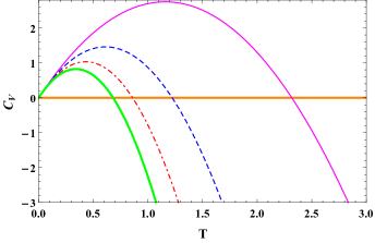
Figure 4: Heat capacity as a function of the temperature and considering the influence of Horndeski gravity for the following values $\theta{{}^{\prime}}=2\pi/3$, $\alpha=-8/3$, with $\gamma^{\prime}=-0.1$ (solid line), $\gamma^{\prime}=-0.2$ (dashed line), $\gamma^{\prime}=-0.3$ (dot dashed line), and $\gamma^{\prime}=-0.4$ (thick line).

The sound speed is defined as:

$$c_{s}^{2}\equiv\frac{\partial p}{\partial\epsilon}=\frac{\partial T}{\partial\epsilon}\frac{\partial p}{\partial T}\,.$$ (72)

Identifying

$$\frac{\partial T}{\partial\epsilon}=\left(\frac{\partial\epsilon}{\partial T}\right)^{-1}=C_{V}^{-1}\,;\qquad\frac{\partial p}{\partial T}=S\,,$$ (73)

one gets:

$$c_{s}^{2} = \frac{S}{C_{V}}\,.$$ (74)

In Fig. 5, we present the behavior of the entropy $S$ and sound speed $c^{2}_{s}$ against the temperature achieved from our model. The entropy comes directly from Eq. (57). In the left panel one can see the behavior of the entropy $S$ and the influence of Horndeski gravity. On the other hand, in the right panel, we show the sound speed and the effects of Horndeski gravity which are more intense for $\gamma^{\prime}=-0.4$. In this case it deviates from the value 1/3 associated with the conformal system.

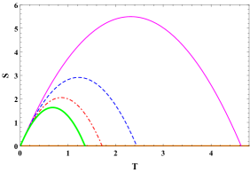
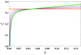
Figure 5: Entropy (left panel) and sound speed (Right panel) as a functions of the temperature and considering the influence of Horndeski gravity for the following values values $\theta{{}^{\prime}}=2\pi/3$, $\alpha=-8/3$, with $\gamma^{\prime}=-0.1$ (solid line), $\gamma^{\prime}=-0.2$ (dashed line), $\gamma^{\prime}=-0.3$ (dot dashed line), and $\gamma^{\prime}=-0.4$ (thick line).

The last thermodynamic quantity that we present in this section is the trace of the energy-momentum tensor, defined as:

$$\langle T^{a}_{\ \ a}\rangle=\epsilon-3p=4\Omega+TS\,.$$ (75)

In Fig. 6, one can see the behavior of the scaled trace of the energy-momentum tensor ($\langle T^{a}_{\ \ a}\rangle/T^{4}$) as a function of temperature. It exhibits rather interesting behavior: for the small-temperature regime we have $\langle T^{a}_{\ \ a}\rangle\neq 0$., but for the high-temperature regime, despite the influence of Horndeski gravity, $\langle T^{a}_{\ \ a}\rangle\to 0$, which is an indication of a restoration of the conformal symmetry and therefore the emergence of a nontrivial BCFT.

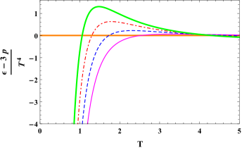
Figure 6: Trace of the scaled energy-momentum tensor as a function of the temperature considering the following values $\theta{{}^{\prime}}=2\pi/3$, $\alpha=-8/3$, with $\gamma^{\prime}=-0.1$ (solid line), $\gamma^{\prime}=-0.2$ (dashed line), $\gamma^{\prime}=-0.3$ (dot dashed line), and $\gamma^{\prime}=-0.4$ (thick line).

VIII Hawking-Page phase transition

In this section, we analyze the HPPT for a BTZ black hole considering the contributions of the AdS/BCFT correspondence within Horndeski gravity. The HPPT was originally proposed in Ref. hawpage , in the context of general relativity, where the authors discussed the stability and instability of black holes in AdS space. The transition between the stable and unstable configurations characterizes a phase transition of first order with an associated critical temperature.

In the context of the AdS/CFT program, the pioneering work in Ref. Witten:1998zw , showed how to relate the temperature in gravitational theory with that associated with the gauge theory on the boundary. For an incomplete list of works dealing with HPPT within the AdS/QCD context see, for instance, Refs. Cho:2002hq ; Herzog:2006ra ; Kajantie:2006hv ; BallonBayona:2007vp ; Rodrigues:2017cha ; Rodrigues:2017iqi ; Chen:2020ath ; Li:2020khm ; Wang:2020pmb . In particular, the HPPT within the BTZ black hole scenario was studied in e.g. Refs. Myung:2006sq ; Eune:2013qs ; Detournay:2015ysa ; Myung:2015pua ; Tang:2016vmu ; Ganai:2019lgc .

The partition function for the AdS-black hole ($V_{E}$) is identified with minus the renormalized Euclidean action, Eq. (52), $V_{E}=-I_{E}$, so that:

$$V_{E} = \frac{L\Delta y}{8r_{h}G_{N}}\left(1-\frac{\xi^{\prime}}{8}\right)+\frac{L\Delta y_{Q}}{2r_{h}G_{N}}\left(1-\frac{\xi^{\prime}}{8}\right)$$ (76)

$$- \frac{\xi^{\prime}b(\theta^{{}^{\prime}})L^{3}}{2r^{2}_{h}G_{N}}\left(1-\frac{\xi^{\prime}}{8}\right)-\frac{\xi^{\prime}q(\theta^{{}^{\prime}})L}{2G_{N}}-\frac{\xi^{\prime}L^{3}h(\theta^{{}^{\prime}})\cot(\theta^{{}^{\prime}})}{2r^{2}_{h}G_{N}}\,.$$

Analogously, the partition function for the thermal AdS, is defined as $V_{E}(0)=-I_{E}(0)$, where $I_{E}(0)$ is given by Eq. (53):

$$V_{E}(0)=\frac{L\Delta y}{8r_{h}G_{N}}\left(1-\frac{\xi^{\prime}}{4}\right)\,.$$ (77)

Now, we can compute $\Delta V_{E}$, so that:

$$\Delta V_{E}=\frac{L\Delta y_{Q}}{r_{h}G_{N}}\left(1-\frac{\xi^{\prime}}{8}\right)-\frac{\xi^{\prime}b(\theta^{{}^{\prime}})L^{3}}{2r^{2}_{h}G_{N}}\left(1-\frac{\xi^{\prime}}{8}\right)-\frac{\xi^{\prime}L^{3}h(\theta^{{}^{\prime}})\cot(\theta^{{}^{\prime}})}{2r^{2}_{h}G_{N}}-\frac{\xi^{\prime}q(\theta^{{}^{\prime}})L}{2G_{N}}\,.$$ (78)

According to the HPPT prescription, the difference $\Delta V_{E}$ vanishes at the phase transition and $\Delta V_{E}<0$ indicates the stability of the black hole. On the other hand, $\Delta V_{E}>0$ points the stability of the thermal AdS space.

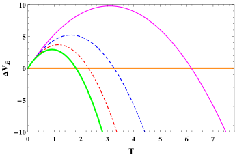
Figure 7: Hawking-Page phase transition from Eq. (78) considering the following values $\theta{{}^{\prime}}=2\pi/3$, $\alpha=-8/3$, with $\gamma^{\prime}=-0.1$ (solid line), $\gamma^{\prime}=-0.2$ (dashed line), $\gamma^{\prime}=-0.3$ (dot dashed line), and $\gamma^{\prime}=-0.4$ (thick line). See the text for discussions.

In Fig. 7, we show the difference between the partition functions as a function of the temperature of the BTZ black hole in the AdS/BCFT correspondence and taking into account the contributions coming from Horndeski gravity. We see that the Horndeski effect decreases the HPPT critical temperature $T_{c}$, where $\Delta V_{E}=0$. Besides, the thermal AdS space is stable for low temperatures ($T<T_{c}$), while the AdS black hole is stable for the high-temperature regime ($T>T_{c}$).

IX Conclusion

In this section we present our conclusions on the AdS/BCFT correspondence and BTZ black hole thermodynamics within Horndeski gravity. Considering the nonminimal coupling between the standard scalar term and the Einstein tensor we established our setup. Besides the three-dimensional bulk, we introduced a Gibbons-Hawking surface term and obtained the corresponding field equations. Then, using the no-hair-theorem, we found a consistent solution for the BTZ black hole. From this solution we constructed the Q profile on the two-dimensional boundary, which characterizes the AdS₃/BCFT₂ correspondence. In particular, we found an exact numerical solution and an approximate analytical one. These two solutions are shown in Fig. 2, where one can see that the approximate solution describes qualitatively well the influence of the Horndeski term. So, starting in Sec. V and all subsequent sections, we only considered the approximated analytical solution. Using this solution, we performed a holographic renormalization procedure in order to get the Euclidean on-shell action for the thermal and the AdS-BTZ black holes. The identification of the Euclidean on-shell action with the free energy allowed us to compute the total entropy which is the sum of the contributions coming from the bulk and boundary both with Horndeski terms. From this total entropy and assuming the Bekenstein-Hawking formula we derived the corresponding total area for the AdS-BTZ black hole with Horndeski terms. We found that the total area grows with the absolute value of $\xi^{\prime}$. This suggests that the information encoded on the black hole horizon also grows with $|\xi^{\prime}|$. Another interpretation for the total entropy found in this work is that it represents a correction to the Bekenstein-Hawking formula. For the boundary entropy, it is remarkable that the influence of Horndeski gravity implies a nonzero or residual entropy in the zero-temperature limit $(r_{h}\to\infty)$, for a certain range of the angle $\theta^{\prime}$. For another range of $\theta^{\prime}$ the limit $T\to 0$ cannot be reached. In this case there it seems that there should be a minimum nonzero temperature corresponding to zero entropy.

The free energy of the AdS-BTZ black hole with Horndeski gravity is depicted in Fig. 3. This picture shows the stability of these solutions for $\Omega<0$, up to a certain critical temperature depending on the Horndeski parameter $\xi^{\prime}$. From this free energy we extracted the other relevant thermodynamic quantities, including the heat capacity, sound speed and trace anomaly. These results seem to be compatible with the ones expected from usual black hole thermodynamic properties.

In Sec. VIII, we studied the Hawking-Page phase transition in the AdS/BCFT correspondence with Horndeski gravity. The modification coming from the Horndeski contribution allowed us to obtain this phase transition as a function of the temperature, as is usual in higher-dimensional contexts. This contrasts with the description of the HPPT given in Refs. Takayanagi:2011zk ; Fujita:2011fp , where the authors plotted the free energy as a function of the Q profile tension.

Finally, we would like to comment that these theories of extended gravity (such as the Horndeski one) and beyond Einstein’s original proposal where such theories take into account scalar fields and their couplings with gravity or accommodate higher-order terms in curvature invariants may provide new insights into aspects that can deepen our knowledge of the gravity duals of conformal field theories like the AdS/BCFT correspondence.

- (1) T. Takayanagi, “Holographic Dual of BCFT,” Phys. Rev. Lett. 107, 101602 (2011), [arXiv:1105.5165 [hep-th]].
- (2) G. W. Horndeski, “Second-order scalar-tensor field equations in a four-dimensional space”, Int. J. Theor. Phys.10,363 (1974).
- (3) B. P. Abbott et al. [LIGO Scientific and Virgo], “Observation of Gravitational Waves from a Binary Black Hole Merger,” Phys. Rev. Lett. 116, no.6, 061102 (2016) [arXiv:1602.03837 [gr-qc]].
- (4) S. Capozziello and M. De Laurentis, “Extended Theories of Gravity,” Phys. Rept. 509, 167-321 (2011) [arXiv:1108.6266 [gr-qc]].
- (5) S. Gottlober, H. J. Schmidt and A. A. Starobinsky, “Sixth Order Gravity and Conformal Transformations,” Class. Quant. Grav. 7, 893 (1990)
- (6) F. C. Adams, K. Freese and A. H. Guth, “Constraints on the scalar field potential in inflationary models,” Phys. Rev. D 43, 965-976 (1991)
- (7) L. Amendola, A. Battaglia Mayer, S. Capozziello, F. Occhionero, S. Gottlober, V. Muller and H. J. Schmidt, “Generalized sixth order gravity and inflation,” Class. Quant. Grav. 10, L43-L47 (1993)
- (8) K. i. Maeda, “Towards the Einstein-Hilbert Action via Conformal Transformation,” Phys. Rev. D 39, 3159 (1989)
- (9) D. Wands, “Extended gravity theories and the Einstein-Hilbert action,” Class. Quant. Grav. 11, 269-280 (1994) [arXiv:gr-qc/9307034 [gr-qc]].
- (10) S. Capozziello, R. de Ritis and A. A. Marino, “Recovering the effective cosmological constant in extended gravity theories,” Gen. Rel. Grav. 30, 1247-1272 (1998) [arXiv:gr-qc/9804053 [gr-qc]].
- (11) C. Charmousis, E. J. Copeland, A. Padilla and P. M. Saffin, “General second order scalar-tensor theory, self tuning, and the Fab Four,” Phys. Rev. Lett. 108, 051101 (2012) [arXiv:1106.2000 [hep-th]].
- (12) C. Charmousis, E. J. Copeland, A. Padilla and P. M. Saffin, “Self-tuning and the derivation of a class of scalar-tensor theories,” Phys. Rev. D 85, 104040 (2012) [arXiv:1112.4866 [hep-th]].
- (13) A. A. Starobinsky, S. V. Sushkov and M. S. Volkov, “The screening Horndeski cosmologies,” JCAP 06, 007 (2016) [arXiv:1604.06085 [hep-th]].
- (14) J. P. Bruneton, M. Rinaldi, A. Kanfon, A. Hees, S. Schlogel and A. Fuzfa, “Fab Four: When John and George play gravitation and cosmology,” Adv. Astron. 2012, 430694 (2012) [arXiv:1203.4446 [gr-qc]].
- (15) A. Cisterna and C. Erices, “Asymptotically locally AdS and flat black holes in the presence of an electric field in the Horndeski scenario,” Phys. Rev. D 89, 084038 (2014) [arXiv:1401.4479 [gr-qc]].
- (16) A. Maselli, H. O. Silva, M. Minamitsuji and E. Berti, “Neutron stars in Horndeski gravity,” Phys. Rev. D 93, no.12, 124056 (2016) [arXiv:1603.04876 [gr-qc]].
- (17) L. Heisenberg, “A systematic approach to generalisations of General Relativity and their cosmological implications,” Phys. Rept. 796, 1-113 (2019) [arXiv:1807.01725 [gr-qc]].
- (18) K. Hajian, S. Liberati, M. M. Sheikh-Jabbari and M. H. Vahidinia, “On Black Hole Temperature in Horndeski Gravity,” Phys. Lett. B 812, 136002 (2021) [arXiv:2005.12985 [gr-qc]].
- (19) J. M. Maldacena, “The Large N limit of superconformal field theories and supergravity,” Int. J. Theor. Phys. 38, 1113 (1999) [Adv. Theor. Math. Phys. 2, 231 (1998)] [hep-th/9711200].
- (20) S. S. Gubser, I. R. Klebanov and A. M. Polyakov, “Gauge theory correlators from noncritical string theory,” Phys. Lett. B 428, 105 (1998), [hep-th/9802109].
- (21) E. Witten, “Anti-de Sitter space and holography,” Adv. Theor. Math. Phys. 2, 253 (1998), [hep-th/9802150].
- (22) O. Aharony, S. S. Gubser, J. M. Maldacena, H. Ooguri and Y. Oz, “Large N field theories, string theory and gravity,” Phys. Rept. 323, 183 (2000), [hep-th/9905111].
- (23) W. J. Jiang, H. S. Liu, H. Lu and C. N. Pope, “DC Conductivities with Momentum Dissipation in Horndeski Theories,” JHEP 07, 084 (2017) [arXiv:1703.00922 [hep-th]].
- (24) M. Baggioli and W. J. Li, “Diffusivities bounds and chaos in holographic Horndeski theories,” JHEP 07, 055 (2017) [arXiv:1705.01766 [hep-th]].
- (25) H. S. Liu, “Violation of Thermal Conductivity Bound in Horndeski Theory,” Phys. Rev. D 98, no.6, 061902 (2018) [arXiv:1804.06502 [hep-th]].
- (26) Y. Z. Li and H. Lu, “-theorem for Horndeski gravity at the critical point,” Phys. Rev. D 97, no.12, 126008 (2018) [arXiv:1803.08088 [hep-th]].
- (27) Y. Z. Li, H. Lu and H. Y. Zhang, “Scale Invariance vs. Conformal Invariance: Holographic Two-Point Functions in Horndeski Gravity,” Eur. Phys. J. C 79, no.7, 592 (2019) [arXiv:1812.05123 [hep-th]].
- (28) X. J. Wang, H. S. Liu and W. J. Li, “AC charge transport in holographic Horndeski gravity,” Eur. Phys. J. C 79, no.11, 932 (2019) [arXiv:1909.00224 [hep-th]].
- (29) M. Fujita, T. Takayanagi and E. Tonni, “Aspects of AdS/BCFT,” JHEP 1111, 043 (2011), [arXiv:1108.5152 [hep-th]].
- (30) M. Nozaki, T. Takayanagi and T. Ugajin, Central Charges for BCFTs and Holography, JHEP 06, 066 (2012) [arXiv:1205.1573 [hep-th]].
- (31) M. Fujita, M. Kaminski and A. Karch, “SL(2,Z) Action on AdS/BCFT and Hall Conductivities,” JHEP 1207, 150 (2012), [arXiv:1204.0012 [hep-th]].
- (32) D. Melnikov, E. Orazi and P. Sodano, “On the AdS/BCFT Approach to Quantum Hall Systems,” JHEP 1305, 116 (2013), [arXiv:1211.1416 [hep-th]].
- (33) J. M. Magán, D. Melnikov and M. R. O. Silva, “Black Holes in AdS/BCFT and Fluid/Gravity Correspondence,” JHEP 1411, 069 (2014), [arXiv:1408.2580 [hep-th]].
- (34) J. Erdmenger, M. Flory and M. N. Newrzella, “Bending branes for DCFT in two dimensions,” JHEP 01, 058 (2015) [arXiv:1410.7811 [hep-th]].
- (35) J. Erdmenger, M. Flory, C. Hoyos, M. N. Newrzella and J. M. S. Wu, “Entanglement Entropy in a Holographic Kondo Model,” Fortsch. Phys. 64, 109-130 (2016) [arXiv:1511.03666 [hep-th]].
- (36) M. Flory, “A complexity/fidelity susceptibility -theorem for AdS3/BCFT2,” JHEP 06, 131 (2017) [arXiv:1702.06386 [hep-th]].
- (37) A. Karch and L. Randall, “Locally localized gravity,” JHEP 05, 008 (2001) [arXiv:hep-th/0011156 [hep-th]].
- (38) A. Karch and L. Randall, “Open and closed string interpretation of SUSY CFT’s on branes with boundaries,” JHEP 06, 063 (2001) [arXiv:hep-th/0105132 [hep-th]].
- (39) S. Carlip, “The (2+1)-Dimensional black hole,” Class. Quant. Grav. 12, 2853-2880 (1995) [arXiv:gr-qc/9506079 [gr-qc]].
- (40) M. Banados, C. Teitelboim and J. Zanelli, “The Black hole in three-dimensional space-time,” Phys. Rev. Lett. 69, 1849-1851 (1992) [arXiv:hep-th/9204099 [hep-th]].
- (41) M. Banados, M. Henneaux, C. Teitelboim and J. Zanelli, “Geometry of the (2+1) black hole,” Phys. Rev. D 48, 1506-1525 (1993) [erratum: Phys. Rev. D 88, 069902 (2013)] [arXiv:gr-qc/9302012 [gr-qc]].
- (42) T. Kobayashi, “Horndeski theory and beyond: a review,” Rept. Prog. Phys. 82, no.8, 086901 (2019) [arXiv:1901.07183 [gr-qc]].
- (43) F. Brito and F. Santos, “Black branes in asymptotically Lifshitz spacetime and viscosity/entropy ratios in Horndeski gravity,” EPL 129, no.5, 50003 (2020), [arXiv:1901.06770 [hep-th]].
- (44) F. F. Santos, Rotating black hole with a probe string in Horndeski Gravity, Eur. Phys. J. Plus 135, no.10, 810 (2020) [arXiv:2005.10983 [hep-th]].
- (45) G. Compere and D. Marolf, “Setting the boundary free in AdS/CFT,” Class. Quant. Grav. 25, 195014 (2008) [arXiv:0805.1902 [hep-th]].
- (46) M. Bravo-Gaete and M. Hassaine, “Lifshitz black holes with a time-dependent scalar field in a Horndeski theory,” Phys. Rev. D 89, 104028 (2014), [arXiv:1312.7736 [hep-th]].
- (47) A. Anabalon, A. Cisterna and J. Oliva, “Asymptotically locally AdS and flat black holes in Horndeski theory,” Phys. Rev. D 89, 084050 (2014), [arXiv:1312.3597 [gr-qc]].
- (48) U. Gursoy, M. Jarvinen and G. Nijs, “Holographic QCD in the Veneziano Limit at a Finite Magnetic Field and Chemical Potential,” Phys. Rev. Lett. 120, no.24, 242002 (2018) [arXiv:1707.00872 [hep-th]].
- (49) M. Henningson and K. Skenderis, “The Holographic Weyl anomaly,” JHEP 07, 023 (1998) [arXiv:hep-th/9806087 [hep-th]].
- (50) J. de Boer, E. P. Verlinde and H. L. Verlinde, “On the holographic renormalization group,” JHEP 08, 003 (2000) [arXiv:hep-th/9912012 [hep-th]].
- (51) S. Das, S. Shankaranarayanan and S. Sur, “Entanglement and corrections to Bekenstein-Hawking entropy,” [arXiv:1002.1129 [gr-qc]].
- (52) A. Almheiri, T. Hartman, J. Maldacena, E. Shaghoulian and A. Tajdini, “The entropy of Hawking radiation,” [arXiv:2006.06872 [hep-th]].
- (53) S. H. Hendi and A. Sheykhi, “Entropic Corrections to Einstein Equations,” Phys. Rev. D 83, 084012 (2011) [arXiv:1012.0381 [hep-th]].
- (54) S. N. Solodukhin, “Entanglement entropy of black holes,” Living Rev. Rel. 14, 8 (2011) [arXiv:1104.3712 [hep-th]].
- (55) K. Bamba, M. Jamil, D. Momeni and R. Myrzakulov, “Generalized Second Law of Thermodynamics in Gravity with Entropy Corrections,” Astrophys. Space Sci. 344, 259-267 (2013) [arXiv:1202.6114 [physics.gen-ph]].
- (56) X. H. Feng, H. S. Liu, H. Lü and C. N. Pope, “Black Hole Entropy and Viscosity Bound in Horndeski Gravity,” JHEP 11, 176 (2015) [arXiv:1509.07142 [hep-th]].
- (57) S. W. Hawking, “Gravitational radiation from colliding black holes,” Phys. Rev. Lett. 26, 1344 (1971).
- (58) J. M. Bardeen, B. Carter and S. W. Hawking, “The Four laws of black hole mechanics,” Commun. Math. Phys. 31, 161 (1973).
- (59) J. D. Bekenstein, “Black holes and entropy,” Phys. Rev. D 7, 2333 (1973).
- (60) A. Chamblin, R. Emparan, C. V. Johnson and R. C. Myers, “Charged AdS black holes and catastrophic holography,” Phys. Rev. D 60, 064018 (1999) [hep-th/9902170].
- (61) A. Chamblin, R. Emparan, C. V. Johnson and R. C. Myers, “Holography, thermodynamics and fluctuations of charged AdS black holes,” Phys. Rev. D 60, 104026 (1999) [hep-th/9904197].
- (62) D. Kubiznak, R. B. Mann and M. Teo, “Black hole chemistry: thermodynamics with lambda,” Class. Quant. Grav. 34, no.6, 063001 (2017) [arXiv:1608.06147 [hep-th]].
- (63) M. Bravo-Gaete and M. Hassaine, “Thermodynamics of a BTZ black hole solution with an Horndeski source,” Phys. Rev. D 90, no.2, 024008 (2014) [arXiv:1405.4935 [hep-th]].
- (64) S. He, L. F. Li and X. X. Zeng, “Holographic van der Waals-like phase transition in the Gauss–Bonnet gravity,” Nucl. Phys. B 915, 243 (2017) [arXiv:1608.04208 [hep-th]].
- (65) S. S. Gubser and A. Nellore, “Mimicking the QCD equation of state with a dual black hole,” Phys. Rev. D 78, 086007 (2008) [arXiv:0804.0434 [hep-th]].
- (66) S. S. Gubser, A. Nellore, S. S. Pufu and F. D. Rocha, “Thermodynamics and bulk viscosity of approximate black hole duals to finite temperature quantum chromodynamics,” Phys. Rev. Lett. 101, 131601 (2008) [arXiv:0804.1950 [hep-th]].
- (67) D. Li, S. He, M. Huang and Q. S. Yan, “Thermodynamics of deformed AdS5 model with a positive/negative quadratic correction in graviton-dilaton system,” JHEP 09, 041 (2011) [arXiv:1103.5389 [hep-th]].
- (68) R. G. Cai, S. He and D. Li, “A hQCD model and its phase diagram in Einstein-Maxwell-Dilaton system,” JHEP 1203, 033 (2012) [arXiv:1201.0820 [hep-th]].
- (69) S. He, S. Y. Wu, Y. Yang and P. H. Yuan, “Phase Structure in a Dynamical Soft-Wall Holographic QCD Model,” JHEP 04, 093 (2013) [arXiv:1301.0385 [hep-th]].
- (70) R. Zhao, H. H. Zhao, M. S. Ma and L. C. Zhang, “On the critical phenomena and thermodynamics of charged topological dilaton AdS black holes,” Eur. Phys. J. C 73, 2645 (2013) [arXiv:1305.3725 [gr-qc]].
- (71) D. Li, J. Liao and M. Huang, “Enhancement of jet quenching around phase transition: result from the dynamical holographic model,” Phys. Rev. D 89, no. 12, 126006 (2014) [arXiv:1401.2035 [hep-ph]].
- (72) Z. Li, Y. Chen, D. Li and M. Huang, “Locating the QCD critical end point through the peaked baryon number susceptibilities along the freeze-out line,” Chin. Phys. C 42, no.1, 013103 (2018) [arXiv:1706.02238 [hep-ph]].
- (73) D. M. Rodrigues, D. Li, E. Folco Capossoli and H. Boschi-Filho, “Chiral symmetry breaking and restoration in 2+1 dimensions from holography: Magnetic and inverse magnetic catalysis,” Phys. Rev. D 98, no.10, 106007 (2018) [arXiv:1807.11822 [hep-th]].
- (74) X. Chen, D. Li and M. Huang, “Criticality of QCD in a holographic QCD model with critical end point,” Chin. Phys. C 43, no.2, 023105 (2019) [arXiv:1810.02136 [hep-ph]].
- (75) X. Chen, D. Li, D. Hou and M. Huang, “Quarkyonic phase from quenched dynamical holographic QCD model,” JHEP 03, 073 (2020) [arXiv:1908.02000 [hep-ph]].
- (76) D. M. Rodrigues, D. Li, E. Folco Capossoli and H. Boschi-Filho, “Holographic Description of Chiral Symmetry Breaking in a Magnetic Field in 2+1 Dimensions with an Improved Dilaton,” EPL 128, no.6, 61001 (2019) [arXiv:1811.04117 [hep-ph]].
- (77) I. Y. Aref’eva, K. Rannu and P. Slepov, [arXiv:2011.07023 [hep-th]].
- (78) A. Ballon-Bayona, H. Boschi-Filho, E. F. Capossoli and D. M. Rodrigues, “Criticality from Einstein-Maxwell-dilaton holography at finite temperature and density,” Phys. Rev. D 102, no.12, 126003 (2020) [arXiv:2006.08810 [hep-th]].
- (79) I. Y. Aref’eva, K. Rannu and P. Slepov, “Energy Loss in Holographic Anisotropic Model for Heavy Quarks in External Magnetic Field,” [arXiv:2012.05758 [hep-th]].
- (80) N. G. Caldeira, E. Folco Capossoli, C. A. D. Zarro and H. Boschi-Filho, “Fluctuation and dissipation from a deformed string/gauge duality model,” Phys. Rev. D 102, no.8, 086005 (2020) [arXiv:2007.00160 [hep-th]].
- (81) D. M. Rodrigues, D. Li, E. Folco Capossoli and H. Boschi-Filho, “Finite density effects on chiral symmetry breaking in a magnetic field in 2+1 dimensions from holography,” Phys. Rev. D 103, no.6, 066022 (2021) [arXiv:2010.06762 [hep-th]].
- (82) N. G. Caldeira, E. Folco Capossoli, C. A. D. Zarro and H. Boschi-Filho, “Fluctuation and dissipation within a deformed holographic model with backreaction,” Phys. Lett. B 815, 136140 (2021) [arXiv:2010.15293 [hep-th]].
- (83) O. DeWolfe, S. S. Gubser and C. Rosen, “A holographic critical point,” Phys. Rev. D 83, 086005 (2011) [arXiv:1012.1864 [hep-th]].
- (84) Y. S. Myung, “Phase transitions of the BTZ black hole in new massive gravity,” Adv. High Energy Phys. 2015, 478273 (2015) [arXiv:1510.02853 [gr-qc]].
- (85) P. A. Ganai, Nadeem-ul-islam and S. Upadhyay, “A report on thermodynamics of charged Rotating BTZ black hole,” [arXiv:1912.00767 [gr-qc]].
- (86) M. S. Ma and R. Zhao, “Phase transition and entropy spectrum of the BTZ black hole with torsion,” Phys. Rev. D 89, no.4, 044005 (2014) [arXiv:1310.1491 [gr-qc]].
- (87) S. H. Hendi, S. Panahiyan and R. Mamasani, “Thermodynamic stability of charged BTZ black holes: Ensemble dependency problem and its solution,” Gen. Rel. Grav. 47, no.8, 91 (2015) [arXiv:1507.08496 [gr-qc]].
- (88) S. H. Hendi, B. Eslam Panah and S. Panahiyan, “Massive charged BTZ black holes in asymptotically (a)dS spacetimes,” JHEP 05, 029 (2016) [arXiv:1604.00370 [hep-th]].
- (89) S. W. Hawking and D. N. Page, Commun. Math. Phys.87, 577 (1983)
- (90) E. Witten, “Anti-de Sitter space, thermal phase transition, and confinement in gauge theories,” Adv. Theor. Math. Phys. 2, 505-532 (1998) [arXiv:hep-th/9803131 [hep-th]].
- (91) Y. M. Cho and I. P. Neupane, “Anti-de Sitter black holes, thermal phase transition and holography in higher curvature gravity,” Phys. Rev. D 66, 024044 (2002) [hep-th/0202140].
- (92) C. P. Herzog, “A Holographic Prediction of the Deconfinement Temperature,” Phys. Rev. Lett. 98, 091601 (2007) [arXiv:hep-th/0608151 [hep-th]].
- (93) K. Kajantie, T. Tahkokallio and J. T. Yee, “Thermodynamics of AdS/QCD,” JHEP 01, 019 (2007) [arXiv:hep-ph/0609254 [hep-ph]].
- (94) C. A. Ballon Bayona, H. Boschi-Filho, N. R. F. Braga and L. A. Pando Zayas, “On a Holographic Model for Confinement/Deconfinement,” Phys. Rev. D 77, 046002 (2008) [arXiv:0705.1529 [hep-th]].
- (95) D. M. Rodrigues, E. Folco Capossoli and H. Boschi-Filho, “Deconfinement phase transition in a magnetic field in 2 + 1 dimensions from holographic models,” Phys. Lett. B 780, 37-40 (2018) [arXiv:1709.09258 [hep-th]].
- (96) D. M. Rodrigues, E. Folco Capossoli and H. Boschi-Filho, “Magnetic catalysis and inverse magnetic catalysis in ( 2+1 )-dimensional gauge theories from holographic models,” Phys. Rev. D 97, no.12, 126001 (2018) [arXiv:1710.07310 [hep-th]].
- (97) X. Chen, L. Zhang, D. Li, D. Hou and M. Huang, “Gluodynamics and deconfinement phase transition under rotation from holography,” arXiv:2010.14478 [hep-ph].
- (98) R. Li and J. Wang, “Thermodynamics and kinetics of Hawking-Page phase transition,” Phys. Rev. D 102, no.2, 024085 (2020)
- (99) Y. Y. Wang, B. Y. Su and N. Li, “Hawking–Page phase transitions in four-dimensional Einstein–Gauss–Bonnet gravity,” Phys. Dark Univ. 31, 100769 (2021) [arXiv:2008.01985 [gr-qc]].
- (100) Y. S. Myung, “Phase transition between the BTZ black hole and AdS space,” Phys. Lett. B 638, 515-518 (2006) [arXiv:gr-qc/0603051 [gr-qc]].
- (101) M. Eune, W. Kim and S. H. Yi, “Hawking-Page phase transition in BTZ black hole revisited,” JHEP 03, 020 (2013) [arXiv:1301.0395 [gr-qc]].
- (102) S. Detournay and C. Zwikel, “Phase transitions in warped AdS3 gravity,” JHEP 05, 074 (2015) [arXiv:1504.00827 [hep-th]].
- (103) Z. Y. Tang, C. Y. Zhang, M. Kord Zangeneh, B. Wang and J. Saavedra, “Thermodynamical and dynamical properties of Charged BTZ Black Holes,” Eur. Phys. J. C 77, no.6, 390 (2017) [arXiv:1610.01744 [hep-th]].