A Novel Estimator of Mutual Information for Learning to Disentangle Textual Representations

Abstract

Learning disentangled representations of textual data is essential for many natural language tasks such as fair classification, style transfer and sentence generation, among others. The existent dominant approaches in the context of text data either rely on training an adversary (discriminator) that aims at making attribute values difficult to be inferred from the latent code or rely on minimising variational bounds of the mutual information between latent code and the value attribute. However, the available methods suffer of the impossibility to provide a fine-grained control of the degree (or force) of disentanglement. In contrast to adversarial methods, which are remarkably simple, although the adversary seems to be performing perfectly well during the training phase, after it is completed a fair amount of information about the undesired attribute still remains. This paper introduces a novel variational upper bound to the mutual information between an attribute and the latent code of an encoder. Our bound aims at controlling the approximation error via the Renyi’s divergence, leading to both better disentangled representations and in particular, a precise control of the desirable degree of disentanglement than state-of-the-art methods proposed for textual data. Furthermore, it does not suffer from the degeneracy of other losses in multi-class scenarios. We show the superiority of this method on fair classification and on textual style transfer tasks. Additionally, we provide new insights illustrating various trade-offs in style transfer when attempting to learn disentangled representations and quality of the generated sentence.

1 Introduction

Learning disentangled representations hold a central place to build rich embeddings of high-dimensional data. For a representation to be disentangled implies that it factorizes some latent cause or causes of variation as formulated by Bengio et al. (2013). For example, if there are two causes for the transformations in the data that do not generally happen together and are statistically distinguishable (e.g., factors occur independently), a maximally disentangled representation is expected to present a sparse structure that separates those causes. Disentangled representations have been shown to be useful for a large variety of data, such as video Hsieh et al. (2018), image Sanchez et al. (2019), text John et al. (2018), audio Hung et al. (2018), among others, and applied to many different tasks, e.g., robust and fair classification Elazar and Goldberg (2018), visual reasoning van Steenkiste et al. (2019), style transfer Fu et al. (2017), conditional generation Denton et al. (2017); Burgess et al. (2018), few shot learning Kumar Verma et al. (2018), among others.

In this work, we focus our attention on learning disentangled representations for text, as it remains overlooked by John et al. (2018). Perhaps, one of the most popular applications of disentanglement in textual data is fair classification Elazar and Goldberg (2018); Barrett et al. (2019) and sentence generation tasks such as style transfer John et al. (2018) or conditional sentence generation Cheng et al. (2020b). For fair classification, perfectly disentangled latent representations can be used to ensure fairness as the decisions are taken based on representations which are statistically independent from–or at least carrying limited information about–the protected attributes. However, there exists a trade-offs between full disentangled representations and performances on the target task, as shown by Feutry et al. (2018), among others. For sequence generation and in particular, for style transfer, learning disentangled representations aim at allowing an easier transfer of the desired style. To the best of our knowledge, a depth study of the relationship between disentangled representations based either on adversarial losses solely or on $vCLUB-S$ and quality of the generated sentences remains overlooked. Most of the previous studies have been focusing on either trade-offs between metrics computed on the generated sentences Tikhonov et al. (2019) or performance evaluation of the disentanglement as part of (or convoluted with) more complex modules. This enhances the need to provide a fair evaluation of disentanglement methods by isolating their individual contributions Yamshchikov et al. (2019); Cheng et al. (2020b).
Methods to enforce disentangled representations can be grouped into two different categories. The first category relies on an adversarial term in the training objective that aims at ensuring that sensitive attribute values (e.g. race, sex, style) as statistically independent as possible from the encoded latent representation. Interestingly enough, several works John et al. (2018); Elazar and Goldberg (2018); Bao et al. (2019); Yi et al. (2020); Jain et al. (2019); Zhang et al. (2018); Hu et al. (2017), Elazar and Goldberg (2018) have recently shown that even though the adversary teacher seems to be performing remarkably well during training, after the training phase, a fair amount of information about the sensitive attributes still remains, and can be extracted from the encoded representation. The second category aim at minimising Mutual Information (MI) between encoded latent representation and the sensitive attribute values, i.e., without resorting to an adversarial discriminator. MI acts as an universal measure of dependence since it captures non-linear and statistical dependencies of high orders between the involved quantities Kinney and Atwal (2014). However, estimating MI has been a long-standing challenge, in particular when dealing with high-dimensional data Paninski (2003); Pichler et al. (2020). Recent methods rely on variational upper bounds. For instance, Cheng et al. (2020b) study vCLUB-S Cheng et al. (2020a) for sentence generation tasks. Although this approach improves on previous state-of-the-art methods, it does not allow to fine-tuning of the desired degree of disentanglement, i.e., it enforces light or strong levels of disentanglement where only few features relevant to the input sentence remain (see Feutry et al. (2018) for further discussion).

1.1 Our Contributions

We develop new tools to build disentangled textual representations and evaluate them on fair classification and two sentence generation tasks, namely, style transfer and conditional sentence generation. Our main contributions are summarized below:

• A novel objective to train disentangled representations from attributes. To overcome some of the limitations of both adversarial losses and vCLUB-S we derive a novel upper bound to the MI which aims at correcting the approximation error via either the Kullback-Leibler Ali and Silvey (1966) or Renyi Rényi et al. (1961) divergences. This correction terms appears to be a key feature to fine-tuning the degree of disentanglement compared to vCLUB-S.

• Applications and numerical results. First, we demonstrate that the aforementioned surrogate is better suited than the widely used adversarial losses as well as vCLUB-S as it can provide better disentangled textual representations while allowing fine-tuning of the desired degree of disentanglement. In particular, we show that our method offers a better accuracy versus disentanglement trade-offs for fair classification tasks. We additionally demonstrate that our surrogate outperforms both methods when learning disentangled representations for style transfer and conditional sentence generation while not suffering (or degenerating) when the number of classes is greater than two, which is an apparent limitation of adversarial training. By isolating the disentanglement module, we identify and report existing trade-offs between different degree of disentanglement and quality of generated sentences. The later includes content preservation between input and generated sentences and accuracy on the generated style.

2 Main Definitions and Related Works

We introduce notations, tasks, and closely related work. Consider a training set $\mathcal{D}=\{(x_{i},y_{i})\}_{i=1}^{n}$ of $n$ sentences $x_{i}\in\mathcal{X}$ paired with attribute values $y_{i}\in\mathcal{Y}\equiv\{1,\dots,|\mathcal{Y}|\}$ which indicates a discrete attribute to be disentangled from the resulting representations. We study the following scenarios:

Disentangled representations. Learning disentangled representations consists in learning a model $\mathcal{M}:\mathcal{X}\rightarrow\mathcal{R}^{d}$ that maps feature inputs $X$ to a vector of dimension $d$ that retains as much as possible information of the original content from the input sentence but as little as possible about the undesired attribute $Y$. In this framework, content is defined as any relevant information present in $X$ that does not depend on $Y$.

Applications to binary fair classification. The task of fair classification through disentangled representations aims at building representations that are independent of selective discrete (sensitive) attributes (e.g., gender or race). This task consists in learning a model $\mathcal{M}:\mathcal{X}\rightarrow\{0,1\}$ that maps any input $x$ to a label $l\in\{0,1\}$. The goal of the learner is to build a predictor that assigns each $x$ to either $0$ or $1$ “oblivious” of the protected attribute $y$. Recently, much progress has been made on devising appropriate means of fairness, e.g., Zemel et al. (2013); Zafar et al. (2017); Mohri et al. (2019). In particular, Xie et al. (2017); Barrett et al. (2019); Elazar and Goldberg (2018) approach the problem based on adversarial losses. More precisely, these approaches consist in learning an encoder that maps $x$ into a representation vector $h_{x}$, a critic $C_{\theta_{c}}$ which attempts to predict $y$, and an output classifier $f_{\theta_{d}}$ used to predict $l$ based on the observed $h_{x}$. The classifier is said to be fair if there is no statistical information about $y$ that is present in $h_{x}$ Xie et al. (2017); Elazar and Goldberg (2018).

Applications to conditional sentence generation. The task of conditional sentence generation consists in taking an input text containing specific stylistic properties to then generate a realistic (synthetic) text containing potentially different stylistic properties. It requests to learn a model $\mathcal{M}:\mathcal{X}\times\mathcal{Y}\rightarrow\mathcal{X}$ that maps a pair of inputs $(x,y^{t})$ to a sentence $x^{g}$, where the outcome sentence should retain as much as possible of the original content from the input sentence while having (potentially a new) attribute $y^{g}$. Proposed approaches to tackle textual style transfer Zhang et al. (2020); Xu et al. (2019) can be divided into two main categories. The first category Prabhumoye et al. (2018); Lample et al. (2018) uses cycle losses based on back translation Wieting et al. (2017) to ensure that the content is preserved during the transformation. Whereas, the second category look to explicitly separate attributes from the content. This constraint is enforced using either adversarial training Fu et al. (2017); Hu et al. (2017); Zhang et al. (2018); Yamshchikov et al. (2019) or MI minimisation using vCLUB-S Cheng et al. (2020b). Traditional adversarial training is based on an encoder that aims to fool the adversary discriminator by removing attribute information from the content embedding Elazar and Goldberg (2018). As we will observe, the more the representations are disentangled the easier is to transfer the style but at the same time the less the content is preserved. In order to approach the sequence generation tasks, we build on the Style-embedding Model by John et al. (2018) (StyleEmb) which uses adversarial losses introduced in prior work for these dedicated tasks. During the training phase, the input sentence is fed to a sentence encoder, namely $f_{\theta_{e}}$, while the input style is fed to a separated style encoder, namely $f_{\theta_{e}}^{s}$. During the inference phase, the desired style–potentially different from the input style–is provided as input along with the input sentence.

3 Model and Training Objective

This section describes the proposed approach to learn disentangled representations. We first review MI along with the model overview and then, we derive the variational bound we will use, and discuss connections with adversarial losses.

3.1 Model Overview

The MI is a key concept in information theory for measuring high-order statistical dependencies between random quantities. Given two random variables $Z$ and $Y$, the MI is defined by

$$I(Z;Y)=\mathop{\mathbb{E}_{ZY}}\left[\log\frac{p_{ZY}(Z,Y)}{p_{Z}(Z)p_{Y}(Y)}\right],$$ (1)

where $p_{ZY}$ is the joint probability density function (pdf) of the random variables $(Z,Y)$, with $p_{Z}$ and $p_{Y}$ representing the respective marginal pdfs. MI is related to entropy $h(Y)$ and conditional entropy $h(Y|Z)$ as follows:

$$I(Z;Y)=h(Y)-h(Y|Z).$$ (2)

Our models for fair classification and sequence generation share a similar structure. These rely on an encoder that takes as input a random sentence $X$ and maps it to a random representation $Z$ using a deep encoder denoted by $f_{\theta_{e}}$. Then, classification and sentence generation are performed using either a classifier or an auto-regressive decoder denoted by $f_{\theta_{d}}$. We aim at minimizing MI between the latent code represented by the Random Variable (RV) $Z=f_{\theta_{e}}(X)$ and the desired attribute represented by the RV $Y$. The objective of interest $\mathcal{L}(f_{\theta_{e}})$ is defined as:

$$\mathcal{L}(f_{\theta_{e}})\equiv\underbrace{\mathcal{L}_{down.}(f_{\theta_{e}})}_{\textrm{downstream task}}+\lambda\cdot\underbrace{I(f_{\theta_{e}}(X);Y)}_{\textrm{disentangled}},$$ (3)

where $\mathcal{L}_{down.}$ represents a downstream specific (target task) loss and $\lambda$ is a meta-parameter that controls the sensitive trade-off between disentanglement (i.e., minimizing MI) and success in the downstream task (i.e., minimizing the target loss). In Sec. 5, we illustrate theses different trade-offs.

Applications to fair classification and sentence generation. For fair classification, we follow standard practices and optimize the cross-entropy between prediction and ground-truth labels. In the sentence generation task $\mathcal{L}_{down.}$ represents the negative log-likelihood between individual tokens.

3.2 A Novel Upper Bound on MI

Estimating the MI is a long-standing challenge as the exact computation Paninski (2003) is only tractable for discrete variables, or for a limited family of problems where the underlying data-distribution satisfies smoothing properties, see recent work by Pichler et al. (2020). Different from previous approaches leading to variational lower bounds Belghazi et al. (2018); Hjelm et al. (2018); Oord et al. (2018), in this paper we derive an estimator based on a variational upper bound to the MI which control the approximation error based on the Kullback-Leibler and the Renyi divergences Daudel et al. (2020).

Theorem 1

(Variational upper bound on MI) Let $(Z,Y)$ be an arbitrary pair of RVs with $(Z,Y)\sim p_{ZY}$ according to some underlying pdf, and let $q_{\widehat{Y}|Z}$ be a conditional variational distribution on the attributes satisfying $p_{ZY}\ll p_{Z}\cdot q_{\widehat{Y}|Z}$, i.e., absolutely continuous. Then, we have that

$$\begin{split}&I(Z;Y)\leq\mathbb{E}_{Y}\left[-\log\int q_{\widehat{Y}|Z}(Y|z)p_{Z}(z)dz\right]+\\ &\mathbb{E}_{YZ}\left[\log q_{\widehat{Y}|Z}(Y|Z)\right]+\text{KL}\big{(}p_{ZY}\|p_{Z}\cdot q_{\widehat{Y}|Z}\big{)},\end{split}$$ (4)

where $\textrm{KL}\big{(}p_{ZY}\|p_{Z}\cdot q_{\widehat{Y}|Z}\big{)}$ denotes the KL divergence. Similarly, we have that for any $\alpha>1$,

$$\begin{split}&I(Z;Y)\leq\mathbb{E}_{Y}\left[-\log\int q_{\widehat{Y}|Z}(Y|z)p_{Z}(z)dz\right]+\\ &\mathbb{E}_{YZ}\left[\log q_{\widehat{Y}|Z}(Y|Z)\right]+D_{\alpha}\big{(}p_{ZY}\|p_{Z}\cdot q_{\widehat{Y}|Z}\big{)},\end{split}$$ (5)

where $(\alpha-1)D_{\alpha}\big{(}p_{ZY}\|p_{Z}\cdot q_{\widehat{Y}|Z}\big{)}=\log\mathbb{E}_{ZY}[$ $R^{\alpha-1}(Z,Y)]$ denotes the Renyi divergence and $R(z,y)=\frac{p_{Y|Z}(y|z)}{q_{\widehat{Y}|Z}(y|z)}$, for $(z,y)\in\textrm{Supp}(p_{ZY})$.

Proof: The upper bound on $H(Y)$ is a direct application of the the Donsker and Varadhan (1985) representation of KL divergence while the lower bound on $H(Y|Z)$ follows from the monotonicity property of the function: $\alpha\mapsto D_{\alpha}\big{(}p_{ZY}\|p_{Z}\cdot q_{\widehat{Y}|Z}\big{)}$. Further details are relegated to Appendix A.

Remark: It is worth to emphasise that the KL divergence in equation 4 and Renyi divergence in equation 5 control the approximation error between the exact entropy and its corresponding bound.

From theoretical bounds to trainable surrogates to minimize MI: It is easy to check that the inequalities in (Eq. 4) and (Eq. 5) are tight provided that $p_{ZY}\equiv p_{Z}\cdot q_{\widehat{Y}|Z}$ almost surely for some adequate choice of the variational distribution. However, the evaluation of these bounds requires to obtain an estimate of the density-ratio $R(z,y)$. Density-ratio estimation has been widely studied in the literature (see Sugiyama et al. (2012) and references therein) and confidence bounds has been reported by Kpotufe (2017) under some smoothing assumption on underlying data-distribution $p_{ZY}$. In this work, we will estimate this ratio by using a critic $C_{\theta_{R}}$ which is trained to differentiate between a balanced dataset of positive i.i.d samples coming from $p_{ZY}$ and negative i.i.d samples coming from $q_{\widehat{Y}|Z}\cdot p_{Z}$. Then, for any pair $(z,y)$, the density-ratio can be estimated by $R(z,y)\approx\frac{\sigma(C_{\theta_{R}}(z,y))}{1-\sigma(C_{\theta_{R}}(z,y))}$, where $\sigma(\cdot)$ indicates the sigmoid function and $C_{\theta_{R}}(z,y)$ is the unnormalized output of the critic. It is worth to mention that after estimating this ratio, the previous upper bounds may not be strict bounds so we will refer them as surrogates.

3.3 Comparison to existing methods

Adversarial approaches: In order to enhance our understanding of why the proposed approach based on the minimization of the MI using our variational upper bound in Th. 1 may lead to a better training objective than previous adversarial losses, we discuss below the explicit relationship between MI and cross-entropy loss. Let $Y\in\mathcal{Y}$ denote a random attribute and let $Z$ be a possibly high-dimensional representation that needs to be disentangled from $Y$. Then,

$$\begin{split}I(Z;Y)\,\geq\,&H(Y)-\mathbb{E}_{YZ}\left[\log q_{\widehat{Y}|Z}(Y|Z)\right]\\ \,=\,&\textrm{Const}-\textrm{CE}(\widehat{Y}|Z),\end{split}$$ (6)

where $\textrm{CE}(\widehat{Y}|Z)$ denotes the cross-entropy corresponding to the adversarial discriminator $q_{\widehat{Y}|Z}$, noting that $Y$ comes from an unknown distribution on which we have no influence $H(Y)$ is an unknown constant, and using that the approximation error: $\textrm{KL}\big{(}q_{ZY}\|q_{\widehat{Y}|Z}\cdot p_{Z}\big{)}=\textrm{CE}(\widehat{Y}|Z)-H(Y|Z)$. Eq. 6 shows that the cross-entropy loss leads to a lower bound (up to a constant) on the MI. Although the cross-entropy can lead to good estimates of the conditional entropy, the adversarial approaches for classification and sequence generation by Barrett et al. (2019); John et al. (2018) which consists in maximizing the cross-entropy, induces a degeneracy (unbounded loss) as $\lambda$ increases in the underlying optimization problem. As we will observe in next section, our variational upper bound in Th. 1 can overcome this issue, in particular for $|\mathcal{Y}|>2$.

vCLUB-S: Different from our method, Cheng et al. (2020a) introduce $I_{\text{vCLUB}}$ which is an upper bound on MI defined by

$$\begin{split}I_{\text{vCLUB}}(Y;Z)=&\mathbb{E}_{YZ}[\log p_{Y|Z}(Y|Z)]\\ &-\mathbb{E}_{Y}\mathbb{E}_{Z}[\log p_{Y|Z}(Y|Z)].\end{split}$$ (7)

It would be worth to mention that this bound follows a similar approach to the previously introduced bound in Feutry et al. (2018).

4 Experimental Setting

4.1 Datasets

Fair classification task. We follow the experimental protocol of Elazar and Goldberg (2018). The main task consists in predicting a binary label representing either the sentiment (positive/negative) or the mention. The mention task aims at predicting if a tweet is conversational. Here the considered protected attribute is the race. The dataset has been automatically constructed from DIAL corpus Blodgett et al. (2016) which contained race annotations over $50$ Million of tweets. Sentiment tweets are extracted using a list of predefined emojis and mentions are identified using @mentions tokens. The final dataset contains 160k tweets for the training and two splits of 10K tweets for validation and testing. Splits are balanced such that the random estimator is likely to achieve $50\%$ accuracy. Style Transfer For our sentence generation task, we conduct experiments on three different datasets extracted from restaurant reviews in Yelp. The first dataset, referred to as SYelp, contains 444101, 63483, and 126670 labelled short reviews (at most 20 words) for train, validation, and test, respectively. For each review a binary label is assigned depending on its polarity. Following Lample et al. (2018), we use a second version of Yelp, referred to as FYelp, with longer reviews (at most $70$ words). It contains five coarse-grained restaurant category labels (e.g., Asian, American, Mexican, Bars and Dessert). The multi-category FYelp is used to access the generalization capabilities of our methods to a multi-class scenario.

4.2 Metrics for Performance Evaluation

Efficiency measure of the disentanglement methods. Barrett et al. (2019) report that offline classifiers (post training) outperform clearly adversarial discriminators. We will re-training a classifier on the latent representation learnt by the model and we will report its accuracy.

Measure of performance within the fair classification task. In the fair classification task we aim at maximizing accuracy on the target task and so we will report the corresponding accuracy.

Measure of performance within sentence generation tasks. Sentences generated by the model are expected to be fluent, to preserve the input content and to contain the desired style. For style transfer, the desired style is different from the input style while for conditional sentence generation, both input and output styles should be similar. Nevertheless, automatic evaluation of generative models for text is still an open problem. We measure the style of the output sentence by using a fastText classifier Joulin et al. (2016b). For content preservation, we follow John et al. (2018) and compute both: (i) the cosine measure between source and generated sentence embeddings, which are the concatenation of min, max, and mean of word embedding (sentiment words removed), and (ii) the BLEU score between generated text and the input using SACREBLEU from Post (2018). Motivated by previous work, we evaluate the fluency of the language with the perplexity given by a GPT-2 Radford et al. (2019) pretrained model performing fine-tuning on the training corpus. We choose to report the log-perplexity since we believe it can better reflects the uncertainty of the language model (a small variation in the model loss would induce a large change in the perplexity due to the exponential term). Besides the automatic evaluation, we further test our disentangled representation effectiveness by human evaluation results are presented in Tab. 1.
Conventions and abbreviations. $Adv$ refers to a model trained using the adversarial loss; vCLUB-S, KL refers to a model trained using the vCLUB-S and KL surrogate (see Eq. 14) respectively; and $D_{\alpha}$ refers to a model trained based on the $\alpha$-Renyi surrogate (Eq. 15), for $\alpha\in\{1.3,1.5,1.8\}$.

5 Numerical Results

In this section, we present our results on the fair classification and binary sequence generation tasks, see Ssec. 5.1 and Ssec. 5.2, respectively. We additionally show that our variational surrogates to the MI–contrarily to adversarial losses–do not suffer in multi-class scenarios (see Ssec. 5.3).

5.1 Applications to Fairness

Upper bound on performances. We first examine how much of the protected attribute we can be recovered from an unfair classifier (i.e., trained without adversarial loss) and how well does such classifier perform. Results are reported in Fig. 1. We observe that we achieve similar scores than the ones reported in previous studies Barrett et al. (2019); Elazar and Goldberg (2018). This experiment shows that, when training to solve the main task, the classifier learns information about the protected attribute, i.e., the attacker’s accuracy is better than random guessing. In the following, we compare the different proposed methods to disentangle representations and obtain a fairer classifier.

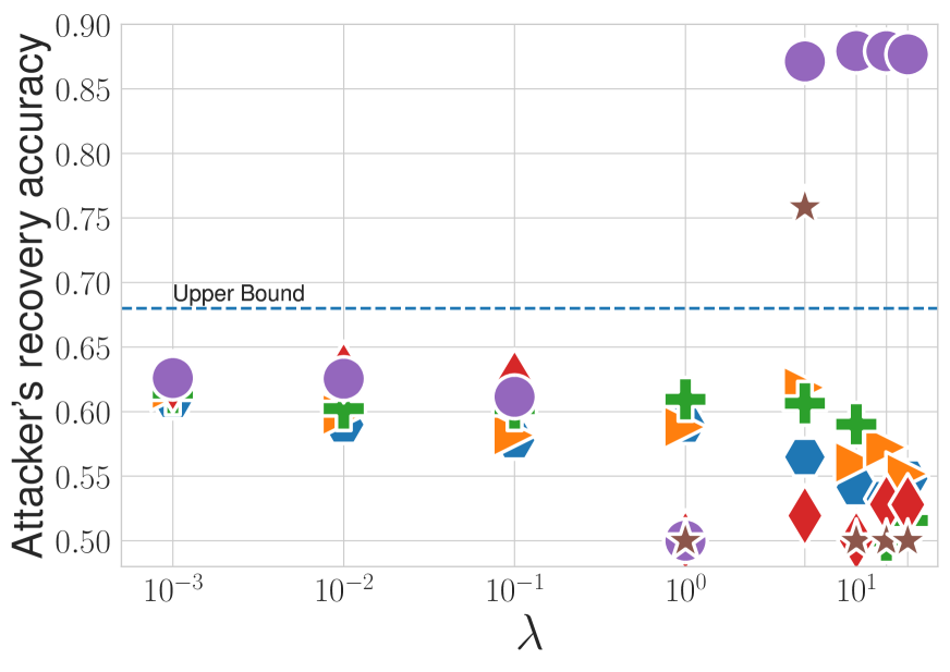
(a)

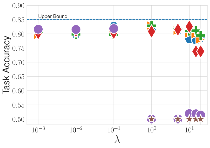
(b)

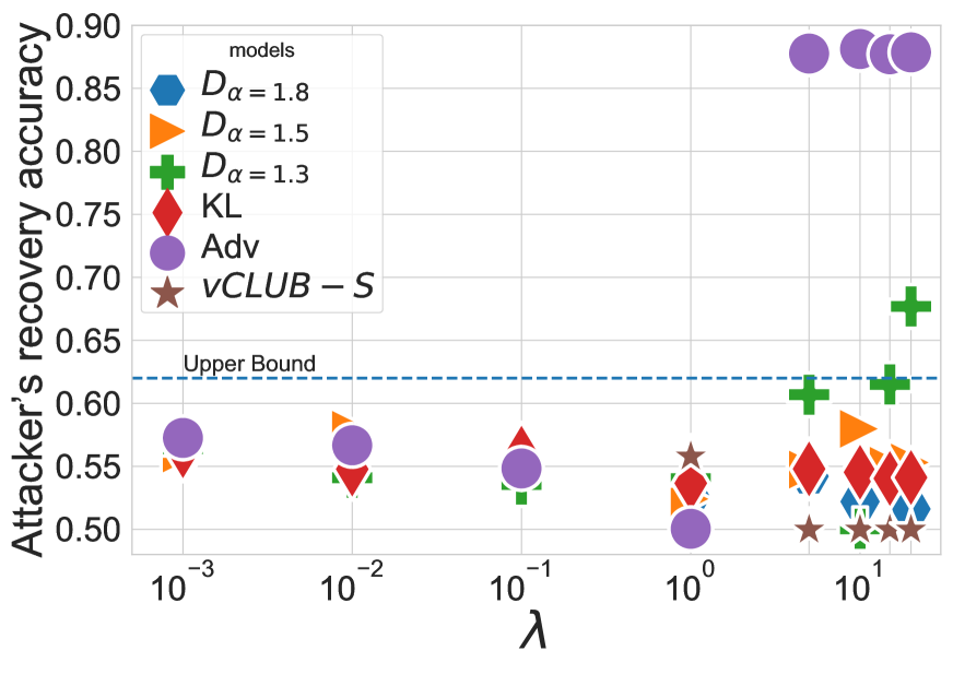
(c)

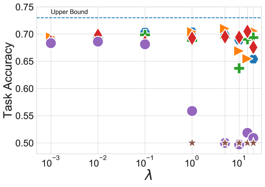
(d)

Figure 1: Numerical results on fair classification. Trade-offs between target task and attacker accuracy are reported in 1(a), 1(b) for mention task, and 1(c), 1(d) for sentiment task. For low values of $\lambda$ some points coincide. As $\lambda$ increases the level of disentanglement increases and the proposed methods using both KL ($KL$) and Reny divergences ($\mathcal{D}_{\alpha}$) clearly offer better control than existing methods.

Methods comparisons. Fig. 1 shows the results of the different models and illustrates the trade-offs between disentangled representations and the target task accuracy. Results are reported on the testset for both sentiment and mention tasks when race is the protected. We observe that the classifier trained with an adversarial loss degenerates for $\lambda>5$ since the adversarial term in Eq. 3 is influencing much the global gradient than the downstream term (i.e., cross-entropy loss between predicted and golden distribution). Remarkably, both models trained to minimize either the KL or the Renyi surrogate do not suffer much from the aforementioned multi-class problem. For both tasks, we observe that the KL and the Renyi surrogates can offer better disentangled representations than those induced by adversarial approaches. In this task, both the KL and Renyi achieve perfect disentangled representations (i.e., random guessing accuracy on protected attributes) with a $5\%$ drop in the accuracy of the target task, when perfectly masking the protected attributes. As a matter of fact, we observe that vCLUB-S provides only two regimes: either a “light” protection (attacker accuracy around 60%), with almost no loss in task accuracy ($\lambda<1$), or a strong protection (attacker accuracy around 50%), where a few features relevant to the target task remain. On the sentiment task, we can draw similar conclusions. However, the Renyi’s surrogate achieves slightly better-disentangled representations. Overall, we can observe that our proposed surrogate enables good control of the degree of disentangling. Additionally, we do not observe a degenerated behaviour–as it is the case with adversarial losses–when $\lambda$ increases. Furthermore, our surrogate allows simultaneously better disentangled representations while preserving the accuracy of the target task.

5.2 Applications to binary polarity transfer

In the previous section, we have shown that the proposed surrogates do not suffer from limitations of adversarial losses and allow to achieve better disentangled representations than existing methods relying on vCLUB-S. Disentanglement modules are a core block for a large number of both style transfer and conditional sentence generation algorithms Tikhonov et al. (2019); Yamshchikov et al. (2019); Fu et al. (2017) that place explicit constraints to force disentangled representations. First, we assess the disentanglement quality and the control over desired level of disentanglement while changing the downstream term, which for the sentence generation task is the cross-entropy loss on individual token. Then, we exhibit the existing trade-offs between quality of generated sentences, measured by the metric introduced in Ssec. 4.2, and the resulting degree of disentanglement. The results are presented for SYelp

5.2.1 Evaluating disentanglement

2(a) shows the adversary accuracy of the different methods as a function of $\lambda$. Similarly to the fair classification task, a fair amount of information can be recovered from the embedding learnt with adversarial loss. In addition, we observe a clear degradation of its performance for values $\lambda>1$. In this setting, the Renyi surrogates achieves consistently better results in terms of disentanglement than the one minimizing the KL surrogate. The curve for Renyi’s surrogates shows that exploring different values of $\lambda$ allows good control of the disentanglement degree. Renyi surrogate generalizes well for sentence generation. Similarly to the fairness task vCLUB-S only offers two regimes: "light" disentanglement with very little polarity transfer and "strong" disentanglement.

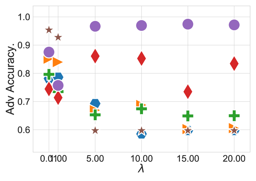
(a) Binary Style Transfert.

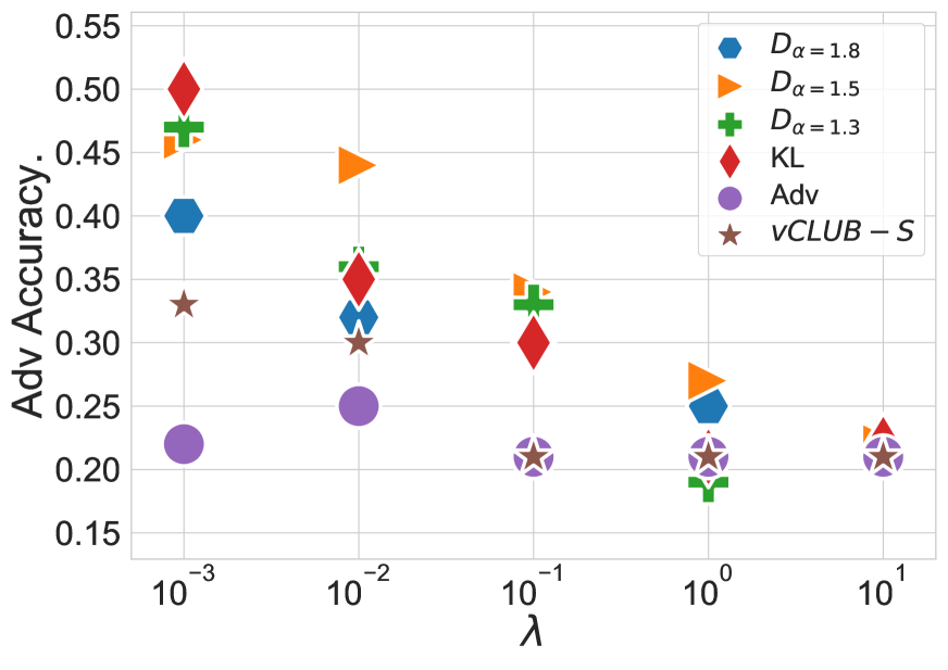
(b) Multiclass Style Transfert

Figure 2: Disentanglement of representation learnt by $f_{\theta_{e}}$ in the binary (left) and multi-class (i.e., $|\mathcal{Y}|=5$) (right) sentence generation scenario. In the multi-class scenario the $Adv$ degenerates for $\lambda\geq 0.01$ and offer no fined-grained control over the degree of disentanglement.

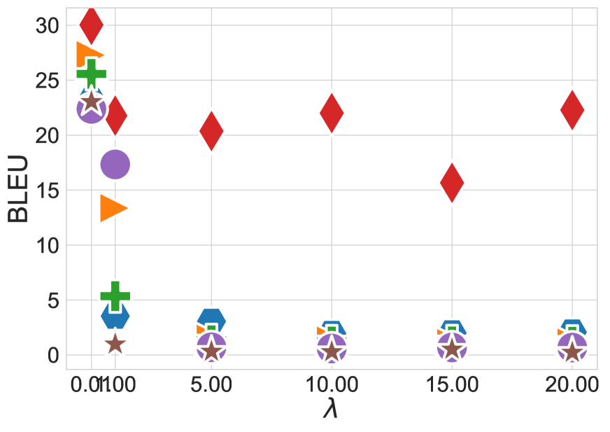
(a)

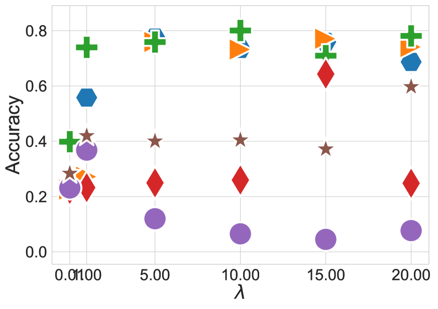
(b)

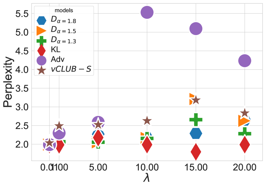
(c)

Figure 3: Numerical experiments on binary style transfer. Quality of generated sentences are evaluated using BLEU (3(a)); style transfer accuracy (3(a)); sentence fluency (3(c)). We report existing trade-offs between disentanglement and sentence generation quality. Human evaluation is reported in Tab. 1.

5.2.2 Disentanglement in Polarity Transfer

The quality of generated sentences are evaluated using the fluency (see 3(c) ), the content preservation (see 3(a)), additional results using a cosine similarity are given in Appendix D, and polarity accuracy (see 3(b) ). For style transfer, and for all models, we observe trade-offs between disentanglement and content preservation (measured by BLEU) and between fluency and disentanglement. Learning disentangled representations leads to poorer content preservation. As a matter of fact, similar conclusions can be drawn while measuring content with the cosine similarity (see Appendix D). For polarity accuracy, in non-degenerated cases (see below), we observe that the model is able to better transfer the sentiment in presence of disentangled representations. Transferring style is easier with disentangled representations, however there is no free lunch here since disentangling also removes important information about the content. It is worth noting that even in the "strong" disentanglement regime vCLUB-S struggles to transfer the polarity (accuracy of 40% for $\lambda\in\{1,2,10,15\}$) where other models reach 80%. It is worth noting that similar conclusions hold for two different sentence generation tasks: style transfer and conditional generation, which tends to validate the current line of work that formulates text generation as generic text-to-text Raffel et al. (2019).
Quality of generated sentences. Examples of generated sentences are given in Tab. 2 , providing qualitative examples that illustrate the previously observed trade-offs. The adversarial loss degenerates for values $\lambda\geq 5$ and a stuttering phenomenon appears Holtzman et al. (2019). Tab. 1 gathers results of human evaluation and show that our surrogates can better disentangle style while preserving more content than available methods.

5.3 Adversarial Loss Fails to Disentangle when $|\mathcal{Y}|\geq 3$

In 2(b) we report the adversary accuracy of our different methods for the values of $\lambda$ using FYelp dataset with category label. In the binary setting for $\lambda\leq 1$, models using adversarial loss can learn disentangled representations while in the multi-class setting, the adversarial loss degenerates for small values of $\lambda$ (i.e sentences are no longer fluent as shown by the increase in perplexity in 4(c)). Minimizing MI based on our surrogates seems to mitigate the problem and offer a better control of the disentanglement degree for various values of $\lambda$ than $vCLUB-S$. Further results are gathered in Appendix G.

6 Summary and Concluding Remarks

We devised a new alternative method to adversarial losses capable of learning disentangled textual representation. Our method does not require adversarial training and hence, it does not suffer in presence of multi-class setups. A key feature of this method is to account for the approximation error incurred when bounding the mutual information. Experiments show better trade-offs than both adversarial training and vCLUB-S on two fair classification tasks and demonstrate the efficiency to learn disentangled representations for sequence generation. As a matter of fact, there is no free-lunch for sentence generation tasks: although transferring style is easier with disentangled representations, it also removes important information about the content.
The proposed method can replace the adversary in any kind of algorithms Tikhonov et al. (2019); Fu et al. (2017) with no modifications. Future work includes testing with other type of labels such as dialog act Chapuis et al. (2020); Colombo et al. (2020), emotions Witon et al. (2018), opinion Garcia et al. (2019) or speaker’s stance and confidence Dinkar et al. (2020). Since it allows more fine-grained control over the amount of disentanglement, we expect it to be easier to tune when combined with more complex models.

7 Acknowledgements

The authors would like to thanks Georg Pichler for the thorough reading. The work of Prof. Pablo Piantanida was supported by the European Commission’s Marie Sklodowska-Curie Actions (MSCA), through the Marie Sklodowska-Curie IF (H2020-MSCAIF-2017-EF-797805).

Appendix A Additional Details On the Surrogates

A.1 Proof of Inequality Eq. 6

In this section, we provide a formal proof of the Eq. 6. Let $(Z,Y)$ be an arbitrary pair of RVs with $(Z,Y)\sim p_{ZY}$ according to some underlying pdf, and let $q_{\widehat{Y}|Z}$ be a conditional variational probability distribution on the discrete attributes satisfying $p_{ZY}\ll p_{Z}\cdot q_{\widehat{Y}|Z}$, i.e., absolutely continuous.

$$I(Z;Y)\geq H(Y)-\textrm{CE}(\widehat{Y}|Z).$$ (8)

Proof: We start by the definition of the MI and use the fact that the maximum entropy distribution is reached for the uniform law in the case of a discrete variable (see Cover and Thomas (2006)).

$$I(Z;Y) =H(Y)-H(Y|Z)$$ (9)

$$=\textrm{Const}-H(Y|Z).$$ (10)

We then need to find the relationship between the cross-entropy and the conditional entropy.

$$\begin{split}&\textrm{KL}(p_{YZ}\|q_{\widehat{Y}Z})\\ &=E_{YZ}\left[\log\frac{p_{Y|Z}(Y|Z)}{q_{\widehat{Y}|Z}(Y|Z)}\right]\\ &=E_{YZ}\big{[}\log p_{{Y}|Z}(Y|Z)\big{]}-E_{YZ}\big{[}\log q_{\widehat{Y}|Z}(Y|Z)\big{]}\\ &=-H(Y|Z)+\textrm{CE}(\widehat{Y}|Z).\end{split}$$ (11)

We know that $\textrm{KL}(p_{YZ}\|q_{\widehat{Y}Z})\geq 0$, thus $\textrm{CE}(\widehat{Y}|Z)\geq H(Y|Z)$ which gives the result.

The underlying hypothesis made by approximating the MI with an adversarial loss is that the contribution of gradient from $\textrm{KL}(p_{YZ}\|q_{\widehat{Y}Z})$ to the bound is negligible.

A.2 Proof of Th. 1

Let $(Z,Y)$ be an arbitrary pair of RVs with $(Z,Y)\sim p_{ZY}$ according to some underlying pdf, and let $q_{\widehat{Y}|Z}$ be a conditional variational probability distribution satisfying $p_{ZY}\ll p_{Z}\cdot q_{\widehat{Y}|Z}$, i.e., absolutely continuous. To obtain an upper bound on the MI we need to upper bound the entropy $H(Y)$ and to lower bound the conditional entropy $H(Y|Z)$.

Upper bound on $H(Y)$. Since the KL divergence is non-negative, we have

$$H(Y)\leq\mathbb{E}_{Y}\left[-\log q_{Y}(Y)\right]$$ (12)

$$=\mathbb{E}_{Y}\left[-\log\int q_{\widehat{Y}|Z}(Y|z)p_{Z}(z)dz\right].$$ (13)

Lower bounds on $H(Y|Z)$. We have the following inequalities:

$$\begin{split}H(Y|Z)&=\mathbb{E}_{YZ}\left[-\log q_{\widehat{Y}|Z}(Y|Z)\right]-\\ &\textrm{KL}(p_{YZ}\|p_{Z}\cdot q_{\widehat{Y}|Z}),\end{split}$$ (14)

where $\textrm{KL}(p_{YZ}\|p_{Z}\cdot q_{\widehat{Y}|Z})$ denotes the KL divergence. Furthermore, for arbitrary values $\alpha>1$,

$$\begin{split}H(Y|Z)\leq&\mathbb{E}_{YZ}\left[-\log q_{\widehat{Y}|Z}(Y|Z)\right]-\\ &D_{\alpha}(p_{YZ}\|p_{Z}\cdot q_{\widehat{Y}|Z}),\end{split}$$ (15)

where ${D}_{\alpha}(p_{YZ}\|p_{Z}\cdot q_{\widehat{Y}|Z})=$

$$\frac{1}{\alpha-1}\log\mathbb{E}_{ZY}\left[R^{\alpha-1}(Z,Y)\right]$$

is the Renyi divergence with

$$R(y,z)=\frac{p_{Y|Z}(y|z)}{q_{\widehat{Y}|Z}(y|z)}.$$

The proof of Eq. 14 is given in Ssec. A.1. In order to show Eq. 15, we remark that Renyi divergence is non-decreasing function $\alpha\mapsto{D}_{\alpha}(p_{ZY}\|p_{Z}\cdot q_{\widehat{Y}|Z})$ in $\alpha\in[0,+\infty)$ (the reader is refereed to Van Erven and Harremos (2014) for a detailed proof). Thus, we have $\forall\alpha>1$,

$$\textrm{KL}(p_{ZY}\|p_{Z}\cdot q_{\widehat{Y}|Z})\leq{D}_{\alpha}(p_{ZY}\|p_{Z}\cdot q_{\widehat{Y}|Z}).$$ (16)

Therefore, from expression Eq. 14 we obtain the desired result.

A.3 Optimization of the Surrogates on MI

In this section, we give details to facilitate the practical implementation of our methods.

A.3.1 Computing the entropy $H(Y)$

$$H(Y) \leq\mathbb{E}_{Y}\left[-\log\int q_{\widehat{Y}|Z}(Y|z)p_{Z}(z)dz\right]$$ (17)

$$\approx\mathbb{E}_{Y}\left[-\log\sum_{i=1}^{n}q_{\widehat{Y}|Z}(Y|z_{i})\right]+\textrm{const.}$$

$$\approx-\frac{1}{|\mathcal{Y}|}\sum_{j=1}^{|\mathcal{Y}|}\log\sum_{i=1}^{n}C_{\theta_{c}}(z_{i})_{y_{j}}+\textrm{const.}$$

where $C_{\theta_{c}}(z_{i})_{y_{j}}$ is the $y_{j}$-th component of the normalised output of the classifier $C_{\theta_{c}}$.

A.3.2 Computing the lower bound on $H(Y|Z)$

The upper bound helds for $\alpha>1$,

$$\begin{split}H(Y|Z)&\approx\textrm{CE}(Y|Z)-\widehat{D}_{\alpha}(p_{ZY}\|p_{Z}\cdot q_{\widehat{Y}|Z})\\ &\approx-\frac{1}{n}\sum_{i=1}^{n}\log q_{\widehat{Y}|Z}(y_{i}|z_{i})-\\ &\frac{1}{\alpha-1}\log\sum_{i=1}^{n}R^{\alpha-1}(z_{i},y_{i}).\end{split}$$ (18)

Estimating the density-ratio $R(z,y)$ In what follows we apply the so-called density-ratio trick to our specific setup. Suppose we have a balanced dataset $\{(y^{p}_{i},z^{p}_{i})\}\sim p_{YZ}$ and $\{(y^{q}_{i},z^{q}_{i})\}\sim q_{\widehat{Y}|Z}p_{Z}$ with $i\in[1,K]$. The density-ratio trick consists in training a classifier $C_{\theta_{R}}$ to distinguish between theses two distribution. Samples coming from $p$ are labelled $u=1$, samples coming from $q$ are labelled $u=0$. Thus, we can rewrite $R(z,y)$ as

$$R(z,y) =\frac{p_{Y|Z}(y,z)}{q_{\widehat{Y}|Z}(y,z)}$$ (19)

$$=\frac{p_{YZ|U}(y,z|u=0)}{p_{YZ|U}(y,z|u=1)}$$ (20)

$$=\frac{p_{U|YZ}(u=0|y,z)}{p_{U|YZ}(u=1|y,z)}\frac{p_{U}(u=1)}{p_{U}(u=0)}$$ (21)

$$=\frac{p_{U|YZ}(u=0|y,z)}{p_{U|YZ}(u=1|y,z)}$$ (22)

$$=\frac{p_{U|YZ}(u=0|y,z)}{1-p_{U|YZ}(u=0|y,z)}.$$ (23)

Obviously, the true posterior distribution $p_{U|YZ}$ is unknown. However, if $C_{\theta_{R}}$ is well trained, then $p_{U|YZ}(u=0|y,z)\approx\sigma(C_{\theta_{R}}(y,z))$, where $\sigma(\cdot)$ denotes the sigmoid function. A detailled procedure for training is given in Algorithm 1.

Algorithm 1 Our method for the fair classification task

1:training dataset for the encoder $\mathcal{D}_{n}=\{(x_{1},y_{1},l_{1}),\;\ldots,\;(x_{n},y_{n},l_{n})\}$, batch size $m$, training dataset for the classifiers and decoder $\mathcal{D^{\prime}}_{n}=\{(x^{\prime}_{1},y^{\prime}_{1},l^{\prime}_{1}),\;\ldots,\;(x^{\prime}_{n},y^{\prime}_{n},l^{\prime}_{n})\}$.

2:parameters $(\theta_{e},\theta_{R},\theta_{c},\theta_{d})$ of the encoder $f_{\theta_{e}}$, classifiers $C_{\theta_{R}}$, $C_{\theta_{c}}$, $f_{\theta_{d}}$

3:

4:while $(\theta_{e},\theta_{R},\theta_{c},\theta_{d})$ not converged do

5:     for  $i\in[1,Unroll]$ do $\triangleright$ Train $C_{\theta_{c}}$, $C_{\theta_{R}}$, $f_{\theta_{d}}$

6:         Sample a batch $\mathcal{B}^{\prime}$ from $\mathcal{D^{\prime}}$

7:         Update ${\theta_{R}}$ based $\mathcal{B}^{\prime}$ and using $C_{\theta_{c}}$

8:         Update ${\theta_{c}}$ with $\mathcal{B}^{\prime}$

9:         Update ${\theta_{d}}$ with $\mathcal{B}^{\prime}$

10:     end for

11:     Sample a batch $\mathcal{B}$ from $\mathcal{D}$ $\triangleright$ Train $f_{\theta_{e}}$

12:     Update $\theta_{e}$ with $\mathcal{B}$ using Eq. 3 with ${\theta_{d}}$.

13:end while

14:$f_{\theta_{e}}$, $f_{\theta_{d}}$

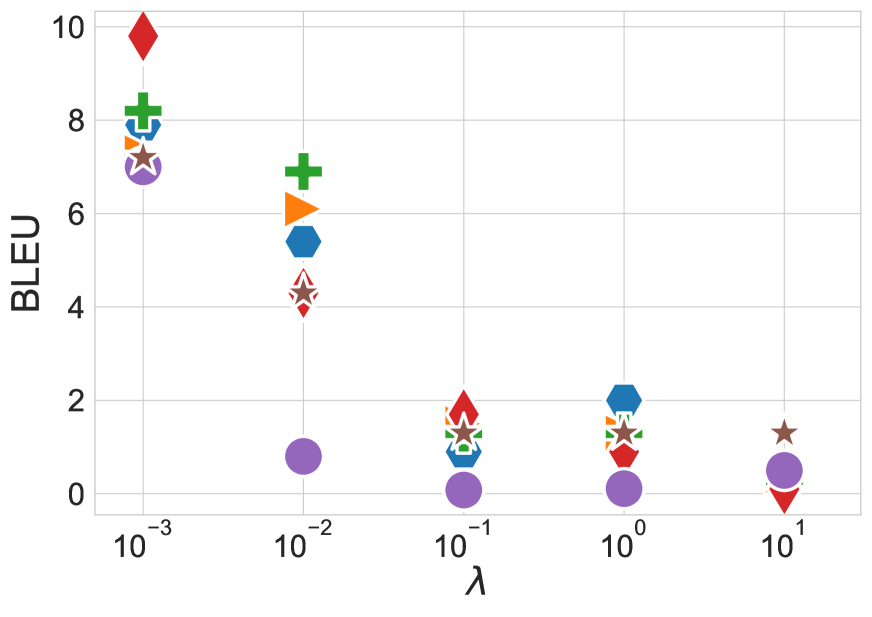
(a)

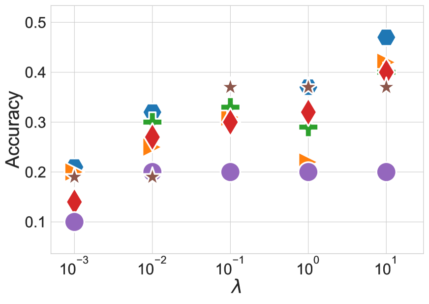
(b)

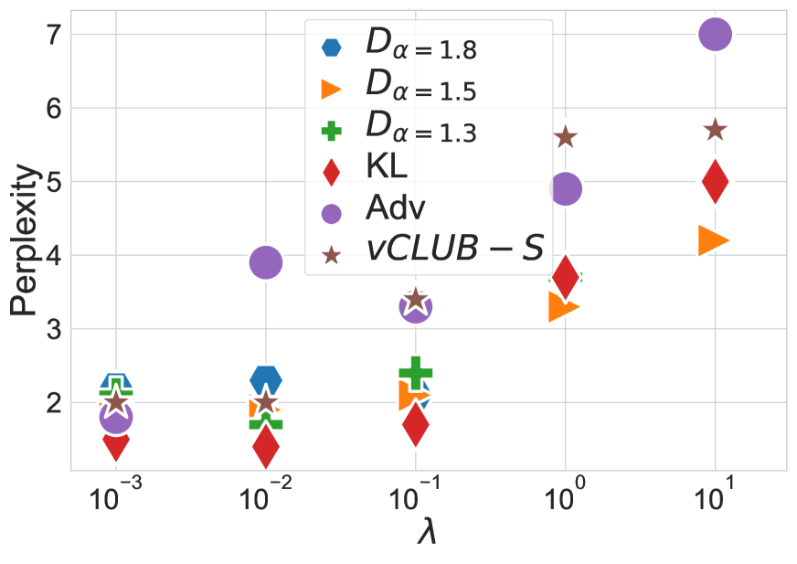
(c)

Figure 4: Numerical experiments on multiclass style transfer using categorical labels. Results include: BLEU (4(a))); style transfer accuracy (4(b)); sentence fluency (4(c)).

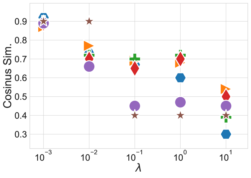
Figure 5: Results of cosine similarity on multiclass style transfer using categorical labels

Appendix B Additional Details on the Model

B.1 Baseline Schemas

We report in Fig. 7 the schema of the proposed approach as well as the baselines.

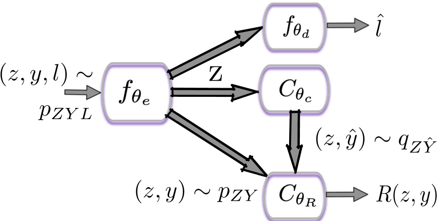
(a) Classifier with our MI surrogate

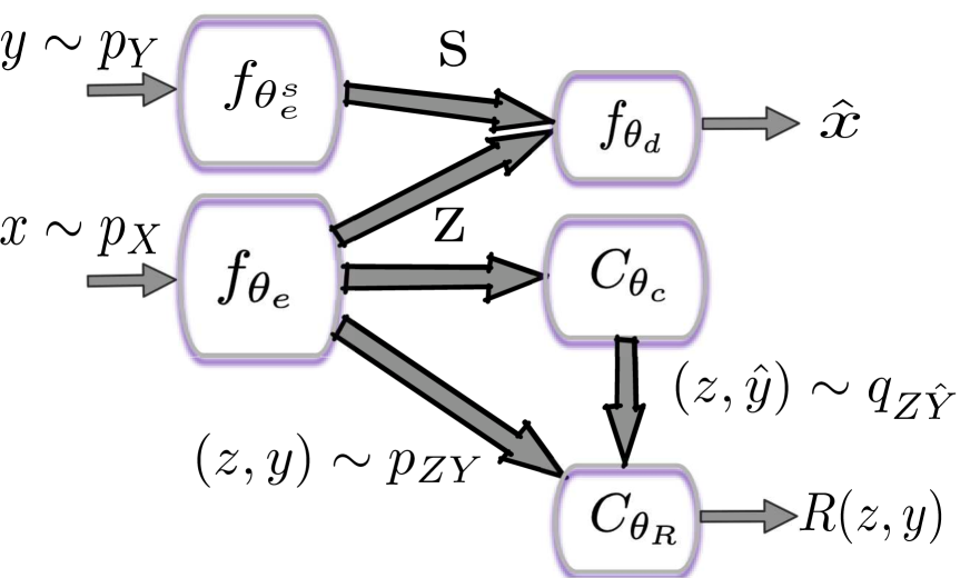
(b) StyleEmb model from John et al. (2018) with our MI surrogate

Figure 6: Proposed methods. As described in Th. 1.

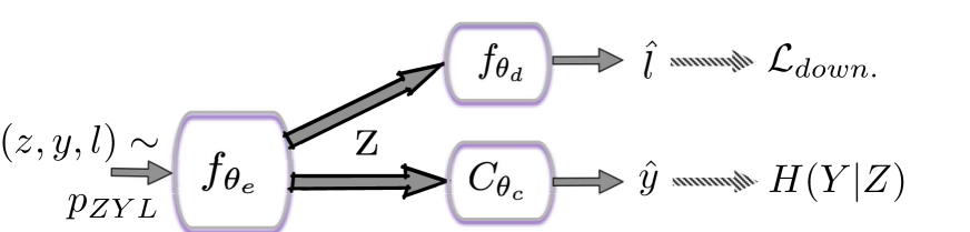
(a) Classifier with adversarial loss from Elazar and Goldberg (2018)

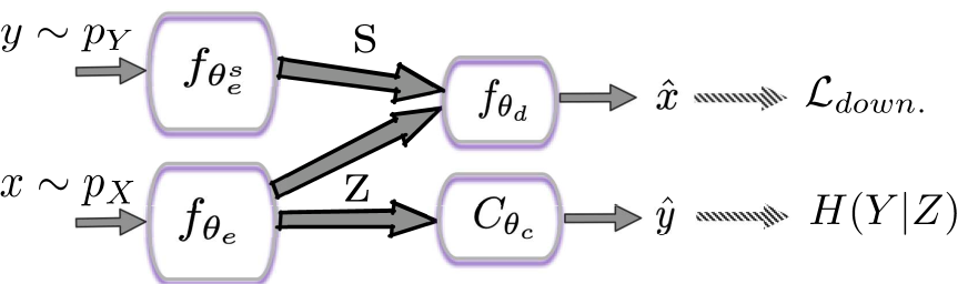
(b) StyleEmb model from John et al. (2018)

Figure 7: Baselines methods, theses models use an adversarial loss for disentanglement. $f_{\theta_{e}}$ represents the input sentence encoder; $f_{\theta_{e}}^{s}$ denotes the style encoder (only used for sentence generation tasks); $C_{\theta_{c}}$ represents the adversarial classifier; $f_{\theta_{d}}$ represents the decoder that can be either a classifier (7(a) or a sequence decoder (7(b)). Schemes of our proposed models are given in LABEL:fig:system

B.2 Architecture Hyerparameters

We use an encoder parameterized by a 2-layer bidirectional GRU Chung et al. (2014) and a 2-layer decoder GRU. Both GRU and our word embedding lookup tables, trained from scratch, and have a dimension of 128 (as already reported by Garcia et al. (2019), building experiments on higher dimensions produces marginal improvement). The style embedding is set to a dimension of 8. The attribute classifier are MLP and are composed of 3 layer MLP with 128 hidden units and LeakyReLU Xu et al. (2015) activations, the dropout Srivastava et al. (2014) rate is set to 0.1. All models are optimised with AdamW Kingma and Ba (2014); Loshchilov and Hutter (2017) with a learning rate of $10^{-3}$ and the norm is clipped to $1.0$. Our model’s hyperparameters have been set by a preliminary training on each downstream task: a simple classifier for the fair classification and a vanilla seq2seq Sutskever et al. (2014); Colombo et al. (2020) for the conditional generation task. The models requested for the classification task are trained during $100k$ steps while 300k steps are used for the generation task.

Appendix C Additional Details on the experimental Setup

In this section, we provide additional details on the metric used for evaluating the different models.

C.1 Content Preservation: BLEU & Cosine Similarity

Content preservation is an important aspect of both conditional sentence generation and style transfer. We provide here the implementation details regarding the implemented metrics.

BLEU. For computing the BLEU score we choose to use the corpus level method provided in python sacrebleu Post (2018) library https://github.com/mjpost/sacrebleu.git. It produces the official WMT scores while working with plain text.

Cosine Similarity. For the cosine similarity, we follow the definition of John et al. (2018) by taking the cosinus between source and generated sentence embedding. For computing the embedding we rely on the bag of word model and take the mean pooling of word embedding. We choose to use the pre-trained word vectors provided in https://fasttext.cc/docs/en/pretrained-vectors.html. They are trained on Wikipedia using fastText. These vectors in dimension 300 were obtained using the skip-gram model described in Bojanowski et al. (2017); Joulin et al. (2016b) with default parameters.

C.2 Fluency: Perplexity

To evaluate fluency we rely on the perplexity Jalalzai et al. (2020), we use GPT-2 Radford et al. (2019) fine-tuned on the training corpus. GPT-2 is pre-trained on the BookCorpus dataset Zhu et al. (2015) (around 800M words). The model has been taken from the HuggingFace Library Wolf et al. (2019). Default hyperparameters have been used for the finetuning.

C.3 Style Conservation/Transfer

For style conservation Colombo et al. (2019) (e.g., polarity, gender or category) we train a fasttext Bojanowski et al. (2017); Joulin et al. (2016a, b) classifier https://fasttext.cc/docs/en/supervised-tutorial.html. We use the validation corpus to select the best model. Preliminary comparisons with deep classifiers (based on either convolutionnal layers or recurrent layers) show that fasttext obtains similar result while being litter and faster.

C.4 Disentanglement

For disentanglement, we follow common practice Lample et al. (2018) and implement a two layers perceptron Rosenblatt (1958). We use LeakyRelu Xu et al. (2015) as activation functions and set the dropout Srivastava et al. (2014) rate to $0.1$.

Appendix D Additional Results on Sentiment

D.1 Binary Sentence Generation

D.1.1 Human Evaluation

In Tab. 1, we report the performances of systems when evaluated by humans on the polarity transfer task. 100 sentences are generated by each system and 3 english native speakers are asked to annotate each sentence along 3 dimensions (i.e fluency, sentiment and content preservation). Turkers assign binary labels to fluency and sentiment (following the protocol introduced in Jalalzai et al. (2020)) while content is evaluated on a likert scale from 1-5. For content preservation, both the input sentence and the generated sentence are provided to the turker. The annotator agreement is measure by the Krippendorff Alpha Krippendorff (2018). The Krippendorff Alpha is: $\alpha=0.54$ on the sentiment classification, $\alpha=0.20$ for fluency and $\alpha=0.18$ for content preservation.

Model	Fluency	Content	Sentiment
Human	0.80	3.4	0.78
$Adv$	0.60	2.4	0.63
$vCLUB-S$	0.62	2.6	0.65
$KL$	0.68	2.6	0.63
$D_{\alpha=1.3}$	0.70	2.4	0.65
$D_{\alpha=1.5}$	0.68	2.9	0.70
$D_{\alpha=1.8}$	0.76	3.0	0.58

Table 1: Human annotation of generated samples. For this comparison we rely on the sentences provided in https://github.com/rpryzant/delete_retrieve_generate. Human annotations are also provided by Li et al. (2018). We have reprocessed the provided sentence using a tokenizer based on SentencePiece Kudo (2018); Sennrich et al. (2016). Since there is a trade-off between automatic evaluation metrics (i.e BLEU, Perplexity and Accuracy of Style Transfer), we set minimum thresholds on BLEU and on style transfert accuracy. The best model that met the threshold on validation is selected. We will release–along with our code–new generated sentences for comparison.

D.2 Content preservation using Cosine Similarity

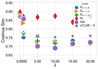
Figure 8: Content preservation measured by the cosine similarity.

Fig. 8 measures the content preservation measured using cosine similarity for the sentence generation task using sentiment labels. As with the BLEU score, we observe that as the learnt representation becomes more entangled ($\lambda$ increases) less content is preserved. Similarly to BLEU the model using the KL bound conserves outperforms other models in terms of content preservation for $\lambda>5$.

D.3 Example of generated sentences

Tab. 2 gathers some sentences generated by the different sentences for different values of $\lambda$.

Style transfert. From Tab. 2, we can observe that the impact of disentanglement on a qualitative point of view. For small values of $\lambda$ the models struggle to do the style transfer (see example 2 for instance). As $\lambda$ increases disentanglement becomes easier, however, the content becomes more generic which is a known problem (see Li et al. (2015) for instance).

Example of “degeneracy" for large values of $\lambda$. For sentences generated with the baseline model a repetition phenomenon appears for greater values of $\lambda$. For certain sentences, models ignore the style token (i.e., the sentence generated with a positive sentiment is the same as the one generated with the negative sentiment). We attribute this degeneracy to the fact that the model is only trained with $(x_{i},y_{i})$ sharing the same sentiment which appears to be an intrinsic limitation of the model introduced by John et al. (2018).

Analysis of performances of vCLUB-S Similarly to what can be observed with automatic evaluation Tab. 2 shows that the system based on vCLUB-S has only two regimes: “light” disentanglement and strong disentanglement. With light disentanglement the decoder fail at transferring the polarity and for strong disentanglement few content features remain and the system tends to output generic sentences.

Appendix E Additional Results on Multi class Sentence Generation

Results on the multi-class style transfer and on are reported in 4(b) Similarly than in the binary case there exists a trade-off between content preservation and style transfer accuracy. We observe that the BLEU score in this task is in a similar range than the one in the gender task, which is expected because data come from the same dataset where only the labels changed.

$\lambda$	Model	Sentence
0.1	Input	It’s freshly made, very soft and flavorful.
	Adv	it’s crispy and too nice and very flavor.
	vCLUB-S	It’s freshly made, and great.
	KL	it’s a huge, crispy and flavorful.
	$D_{\alpha=1.3}$	it’s hard, and the flavor was flavorless.
	$D_{\alpha=1.5}$	it’s very dry and not very flavorful either.
	$D_{\alpha=1.8}$	it’s a good place for lunch or dinner.
1	Input	it’s freshly made, very soft and flavorful.
	Adv	it’s not crispy and not very flavorful flavor.
	vCLUB-S	It’s bad.
	KL	it’s very fresh, and very flavorful and flavor.
	$D_{\alpha=1.3}$	it’s not good, but the prices are good.
	$D_{\alpha=1.5}$	it’s not very good, and the service was terrible.
	$D_{\alpha=1.8}$	it was a very disappointing experience and the food was awful.
5	Input	it’s freshly made, very soft and flavorful.
	Adv	i hate this place.
	vCLUB-S	i hate it.
	KL	it’s very fresh, flavorful and flavorful.
	$D_{\alpha=1.3}$	it’s not worth the money, but it was wrong.
	$D_{\alpha=1.5}$	it’s not worth the price, but not worth it.
	$D_{\alpha=1.8}$	it’s hard to find, and this place is horrible.
10	Input	it’s freshly made, very soft and flavorful.
	Adv	i hate this place.
	vCLUB-S	i hate it.
	KL	it’s a little warm and very flavorful flavor.
	$D_{\alpha=1.3}$	it was a little overpriced and not very good.
	$D_{\alpha=1.5}$	it’s a shame, and the service is horrible.
	$D_{\alpha=1.8}$	it’s not worth the $ NUM.

Table 2: Sequences generated by the different models on the binary sentiment transfer task.

Appendix F Binary Sentence Generation: Application to Gender Data

F.1 Quality of the Disentanglement

In Fig. 9, we report the adversary accuracy of the different methods for the values of $\lambda$. It is worth noting that gender labels are noisier than sentiment labels Lample et al. (2018). We observe that the adversarial loss saturates at $55\%$ where a model trained on MI bounds can achieve a better disentanglement. Additionally, the models trained with MI bounds allow better control of the desired degree of disentanglement.

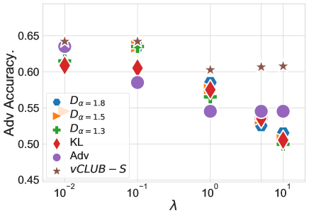
Figure 9: Disentanglement of the learnt embedding when training an off-line adversarial classifier for the sentence generation with gender data.

F.2 Quality of Generated Sentences

Results on the sentence generation tasks are reported in Fig. 10 and in Fig. 11. We observe that for $\lambda>1$ the adversarial loss degenerates as observe in the sentiment experiments.Compared to sentiment score we observe a lower score of BLEU which can be explained by the length of the review in the FYelp dataset. On the other hand, we observe a similar trade-off between style transfer accuracy and content preservation in the non degenerated case: as style transfer accuracy increases, content preservation decreases. Overall, we remark a behaviour similar to the one we observe in sentiment experiments.

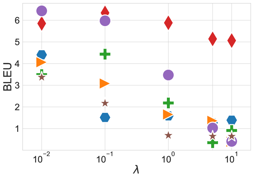
(a)

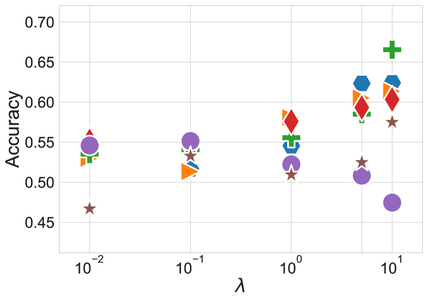
(b)

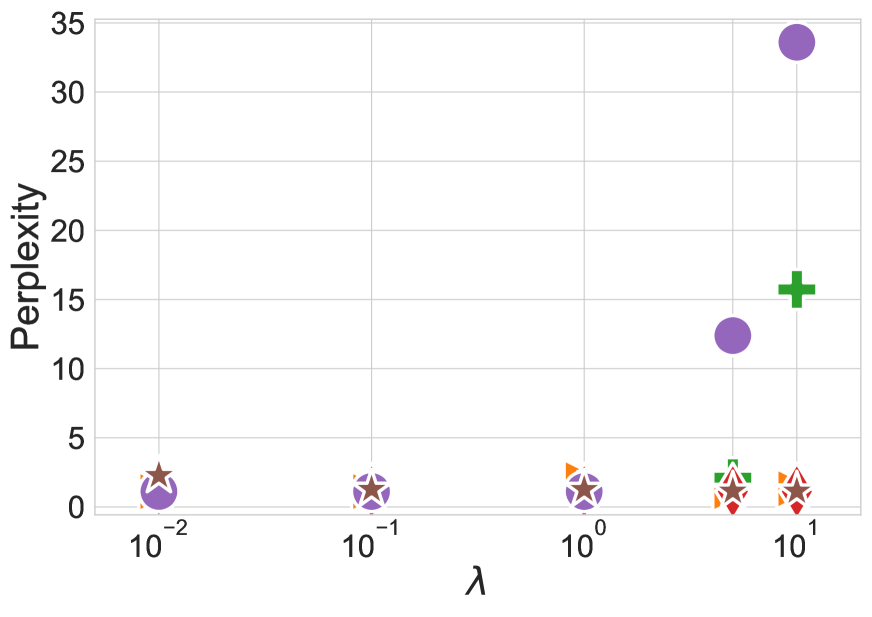
(c)

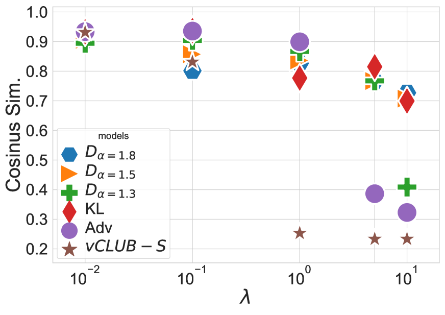
(d)

Figure 10: Numerical experiments on binary style transfer using gender labels. Results include: BLEU (10(a)); cosine similarity (10(d)); style transfer accuracy (10(b)); sentence fluency (10(c)).

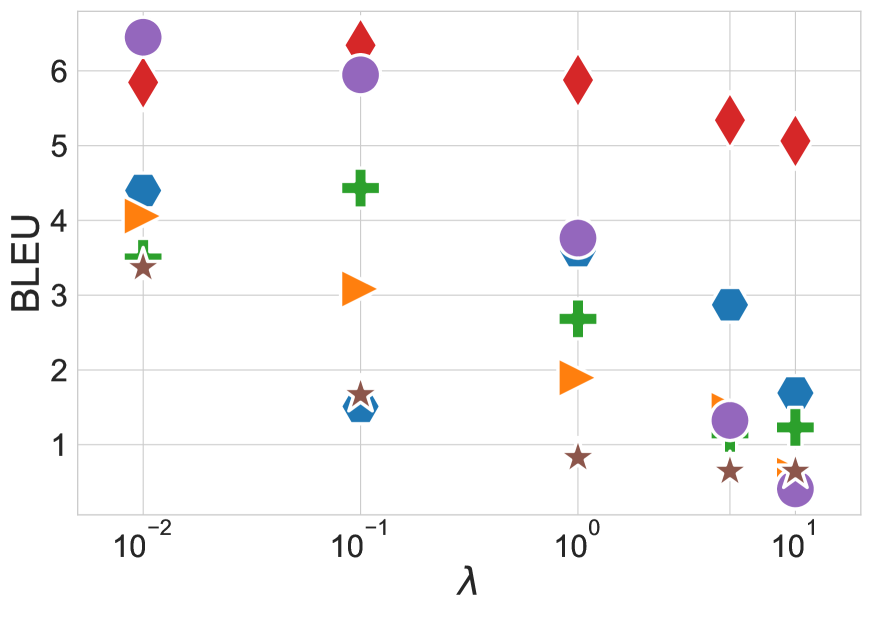
(a)

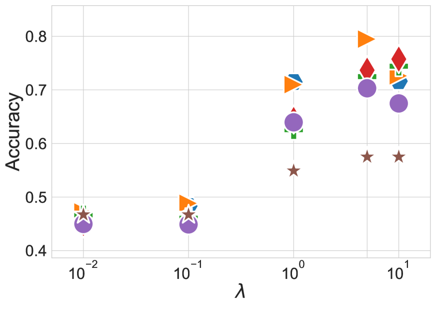
(b)

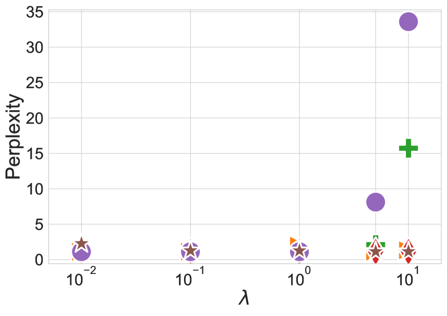
(c)

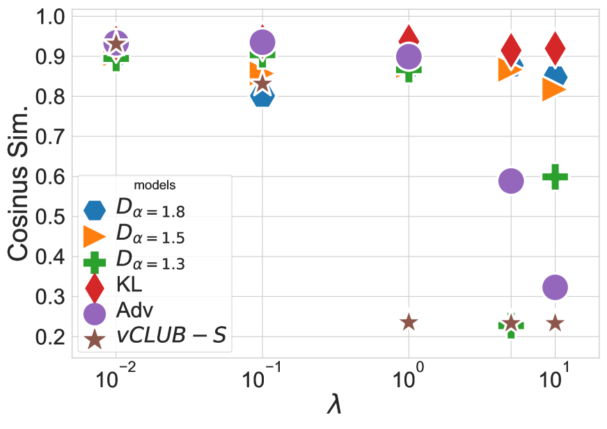
(d)

Figure 11: Numerical experiments on conditional sentence generation using gender labels. Results includes: BLEU (11(a)); cosine similarity (11(d)); style transfer accuracy (11(b)); sentence fluency (11(c)).

Appendix G Additional Results on Multi class Sentence Generation

Results on the multi-class style transfer and on conditional sentence generation are reported in 4(b) and LABEL:fig:accuracy_sentiment_cg. Similarly than in the binary case there exists a trade-off between content preservation and style transfer accuracy. We observe that the BLEU score in this task is in a similar range than the one in the gender task, which is expected because data come from the same dataset where only the labels changed.

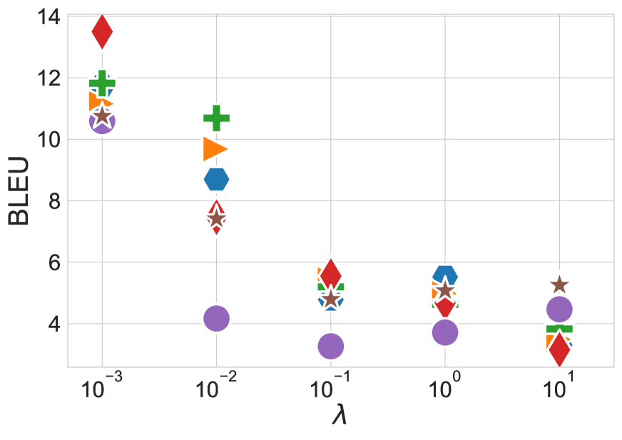
(a)

(b)

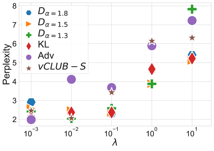
(c)

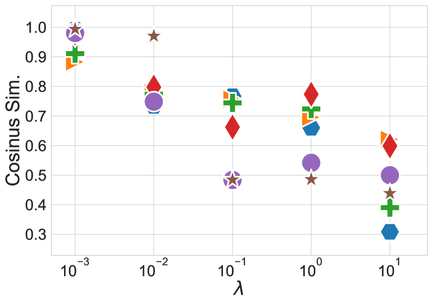
(d)

Figure 12: Numerical experiments on the multi-class conditionnal sentence generation. Results include: BLEU (12(a)); cosine similarity (12(d)); style transfer accuracy (12(b)); sentence fluency (12(c)).

References

- Ali and Silvey (1966) Syed Mumtaz Ali and Samuel D Silvey. 1966. A general class of coefficients of divergence of one distribution from another. Journal of the Royal Statistical Society: Series B (Methodological), 28(1):131–142.
- Bao et al. (2019) Yu Bao, Hao Zhou, Shujian Huang, Lei Li, Lili Mou, Olga Vechtomova, Xinyu Dai, and Jiajun Chen. 2019. Generating sentences from disentangled syntactic and semantic spaces. arXiv preprint arXiv:1907.05789.
- Barrett et al. (2019) Maria Barrett, Yova Kementchedjhieva, Yanai Elazar, Desmond Elliott, and Anders Søgaard. 2019. Adversarial removal of demographic attributes revisited. In Proceedings of the 2019 Conference on Empirical Methods in Natural Language Processing and the 9th International Joint Conference on Natural Language Processing (EMNLP-IJCNLP), pages 6331–6336.
- Belghazi et al. (2018) Mohamed Ishmael Belghazi, Aristide Baratin, Sai Rajeswar, Sherjil Ozair, Yoshua Bengio, Aaron Courville, and R Devon Hjelm. 2018. Mine: mutual information neural estimation. arXiv preprint arXiv:1801.04062.
- Bengio et al. (2013) Y. Bengio, A. Courville, and P. Vincent. 2013. Representation learning: A review and new perspectives. IEEE Transactions on Pattern Analysis and Machine Intelligence, 35(8):1798–1828.
- Blodgett et al. (2016) Su Lin Blodgett, Lisa Green, and Brendan O’Connor. 2016. Demographic dialectal variation in social media: A case study of African-American English. In Proceedings of the 2016 Conference on Empirical Methods in Natural Language Processing, pages 1119–1130, Austin, Texas. Association for Computational Linguistics.
- Bojanowski et al. (2017) Piotr Bojanowski, Edouard Grave, Armand Joulin, and Tomas Mikolov. 2017. Enriching word vectors with subword information. Transactions of the Association for Computational Linguistics, 5:135–146.
- Burgess et al. (2018) Christopher P Burgess, Irina Higgins, Arka Pal, Loic Matthey, Nick Watters, Guillaume Desjardins, and Alexander Lerchner. 2018. Understanding disentangling in -vae. arXiv preprint arXiv:1804.03599.
- Chapuis et al. (2020) Emile Chapuis, Pierre Colombo, Matteo Manica, Matthieu Labeau, and Chloé Clavel. 2020. Hierarchical pre-training for sequence labelling in spoken dialog. In Proceedings of the 2020 Conference on Empirical Methods in Natural Language Processing: Findings, EMNLP 2020, Online Event, 16-20 November 2020, pages 2636–2648. Association for Computational Linguistics.
- Cheng et al. (2020a) Pengyu Cheng, Weituo Hao, Shuyang Dai, Jiachang Liu, Zhe Gan, and Lawrence Carin. 2020a. Club: A contrastive log-ratio upper bound of mutual information. In International Conference on Machine Learning, pages 1779–1788. PMLR.
- Cheng et al. (2020b) Pengyu Cheng, Martin Renqiang Min, Dinghan Shen, Christopher Malon, Yizhe Zhang, Yitong Li, and Lawrence Carin. 2020b. Improving disentangled text representation learning with information-theoretic guidance. arXiv preprint arXiv:2006.00693.
- Chung et al. (2014) Junyoung Chung, Caglar Gulcehre, KyungHyun Cho, and Yoshua Bengio. 2014. Empirical evaluation of gated recurrent neural networks on sequence modeling. arXiv preprint arXiv:1412.3555.
- Colombo et al. (2020) Pierre Colombo, Emile Chapuis, Matteo Manica, Emmanuel Vignon, Giovanna Varni, and Chloe Clavel. 2020. Guiding attention in sequence-to-sequence models for dialogue act prediction. In AAAI, pages 7594–7601.
- Colombo et al. (2019) Pierre Colombo, Wojciech Witon, Ashutosh Modi, James Kennedy, and Mubbasir Kapadia. 2019. Affect-driven dialog generation. arXiv preprint arXiv:1904.02793.
- Cover and Thomas (2006) Thomas M. Cover and Joy A. Thomas. 2006. Elements of Information Theory (Wiley Series in Telecommunications and Signal Processing). Wiley-Interscience, USA.
- Daudel et al. (2020) Kamélia Daudel, Randal Douc, and François Portier. 2020. Infinite-dimensional gradient-based descent for alpha-divergence minimisation. Working paper or preprint.
- Denton et al. (2017) Emily L Denton et al. 2017. Unsupervised learning of disentangled representations from video. In Advances in neural information processing systems, pages 4414–4423.
- Dinkar et al. (2020) Tanvi Dinkar, Pierre Colombo, Matthieu Labeau, and Chloé Clavel. 2020. The importance of fillers for text representations of speech transcripts. In Proceedings of the 2020 Conference on Empirical Methods in Natural Language Processing, EMNLP 2020, Online, November 16-20, 2020, pages 7985–7993. Association for Computational Linguistics.
- Donsker and Varadhan (1985) MD Donsker and SRS Varadhan. 1985. Large deviations for stationary gaussian processes. Communications in Mathematical Physics, 97(1-2):187–210.
- Elazar and Goldberg (2018) Yanai Elazar and Yoav Goldberg. 2018. Adversarial removal of demographic attributes from text data. arXiv preprint arXiv:1808.06640.
- Feutry et al. (2018) Clément Feutry, Pablo Piantanida, Yoshua Bengio, and Pierre Duhamel. 2018. Learning anonymized representations with adversarial neural networks.
- Fu et al. (2017) Zhenxin Fu, Xiaoye Tan, Nanyun Peng, Dongyan Zhao, and Rui Yan. 2017. Style transfer in text: Exploration and evaluation. arXiv preprint arXiv:1711.06861.
- Garcia et al. (2019) Alexandre Garcia, Pierre Colombo, Slim Essid, Florence d’Alché Buc, and Chloé Clavel. 2019. From the token to the review: A hierarchical multimodal approach to opinion mining. arXiv preprint arXiv:1908.11216.
- Hjelm et al. (2018) R Devon Hjelm, Alex Fedorov, Samuel Lavoie-Marchildon, Karan Grewal, Phil Bachman, Adam Trischler, and Yoshua Bengio. 2018. Learning deep representations by mutual information estimation and maximization. arXiv preprint arXiv:1808.06670.
- Holtzman et al. (2019) Ari Holtzman, Jan Buys, Li Du, Maxwell Forbes, and Yejin Choi. 2019. The curious case of neural text degeneration. arXiv preprint arXiv:1904.09751.
- Hsieh et al. (2018) Jun-Ting Hsieh, Bingbin Liu, De-An Huang, Li F Fei-Fei, and Juan Carlos Niebles. 2018. Learning to decompose and disentangle representations for video prediction. In Advances in Neural Information Processing Systems, pages 517–526.
- Hu et al. (2017) Zhiting Hu, Zichao Yang, Xiaodan Liang, Ruslan Salakhutdinov, and Eric P Xing. 2017. Toward controlled generation of text. arXiv preprint arXiv:1703.00955.
- Hung et al. (2018) Yun-Ning Hung, Yi-An Chen, and Yi-Hsuan Yang. 2018. Learning disentangled representations for timber and pitch in music audio. arXiv preprint arXiv:1811.03271.
- Jain et al. (2019) Parag Jain, Abhijit Mishra, Amar Prakash Azad, and Karthik Sankaranarayanan. 2019. Unsupervised controllable text formalization. In Proceedings of the AAAI Conference on Artificial Intelligence, volume 33, pages 6554–6561.
- Jalalzai et al. (2020) Hamid Jalalzai, Pierre Colombo, Chloé Clavel, Eric Gaussier, Giovanna Varni, Emmanuel Vignon, and Anne Sabourin. 2020. Heavy-tailed representations, text polarity classification & data augmentation. arXiv preprint arXiv:2003.11593.
- John et al. (2018) Vineet John, Lili Mou, Hareesh Bahuleyan, and Olga Vechtomova. 2018. Disentangled representation learning for non-parallel text style transfer. arXiv preprint arXiv:1808.04339.
- Joulin et al. (2016a) Armand Joulin, Edouard Grave, Piotr Bojanowski, Matthijs Douze, Hérve Jégou, and Tomas Mikolov. 2016a. Fasttext.zip: Compressing text classification models. arXiv preprint arXiv:1612.03651.
- Joulin et al. (2016b) Armand Joulin, Edouard Grave, Piotr Bojanowski, and Tomas Mikolov. 2016b. Bag of tricks for efficient text classification. arXiv preprint arXiv:1607.01759.
- Kingma and Ba (2014) Diederik P Kingma and Jimmy Ba. 2014. Adam: A method for stochastic optimization. arXiv preprint arXiv:1412.6980.
- Kinney and Atwal (2014) Justin B Kinney and Gurinder S Atwal. 2014. Equitability, mutual information, and the maximal information coefficient. Proceedings of the National Academy of Sciences, 111(9):3354–3359.
- Kpotufe (2017) Samory Kpotufe. 2017. Lipschitz Density-Ratios, Structured Data, and Data-driven Tuning. volume 54 of Proceedings of Machine Learning Research, pages 1320–1328, Fort Lauderdale, FL, USA. PMLR.
- Krippendorff (2018) Klaus Krippendorff. 2018. Content analysis: An introduction to its methodology. Sage publications.
- Kudo (2018) Taku Kudo. 2018. Subword regularization: Improving neural network translation models with multiple subword candidates. arXiv preprint arXiv:1804.10959.
- Kumar Verma et al. (2018) Vinay Kumar Verma, Gundeep Arora, Ashish Mishra, and Piyush Rai. 2018. Generalized zero-shot learning via synthesized examples. In Proceedings of the IEEE conference on computer vision and pattern recognition, pages 4281–4289.
- Lample et al. (2018) Guillaume Lample, Sandeep Subramanian, Eric Smith, Ludovic Denoyer, Marc’Aurelio Ranzato, and Y-Lan Boureau. 2018. Multiple-attribute text rewriting. In International Conference on Learning Representations.
- Li et al. (2015) Jiwei Li, Michel Galley, Chris Brockett, Jianfeng Gao, and Bill Dolan. 2015. A diversity-promoting objective function for neural conversation models. arXiv preprint arXiv:1510.03055.
- Li et al. (2018) Juncen Li, Robin Jia, He He, and Percy Liang. 2018. Delete, retrieve, generate: A simple approach to sentiment and style transfer. arXiv preprint arXiv:1804.06437.
- Loshchilov and Hutter (2017) Ilya Loshchilov and Frank Hutter. 2017. Decoupled weight decay regularization. arXiv preprint arXiv:1711.05101.
- Mohri et al. (2019) Mehryar Mohri, Gary Sivek, and Ananda Theertha Suresh. 2019. Agnostic federated learning. arXiv preprint arXiv:1902.00146.
- Oord et al. (2018) Aaron van den Oord, Yazhe Li, and Oriol Vinyals. 2018. Representation learning with contrastive predictive coding. arXiv preprint arXiv:1807.03748.
- Paninski (2003) Liam Paninski. 2003. Estimation of entropy and mutual information. Neural computation, 15(6):1191–1253.
- Pichler et al. (2020) Georg Pichler, Pablo Piantanida, and Günther Koliander. 2020. On the estimation of information measures of continuous distributions.
- Post (2018) Matt Post. 2018. A call for clarity in reporting bleu scores. arXiv preprint arXiv:1804.08771.
- Prabhumoye et al. (2018) Shrimai Prabhumoye, Yulia Tsvetkov, Ruslan Salakhutdinov, and Alan W Black. 2018. Style transfer through back-translation. arXiv preprint arXiv:1804.09000.
- Radford et al. (2019) Alec Radford, Jeffrey Wu, Rewon Child, David Luan, Dario Amodei, and Ilya Sutskever. 2019. Language models are unsupervised multitask learners. OpenAI Blog, 1(8):9.
- Raffel et al. (2019) Colin Raffel, Noam Shazeer, Adam Roberts, Katherine Lee, Sharan Narang, Michael Matena, Yanqi Zhou, Wei Li, and Peter J Liu. 2019. Exploring the limits of transfer learning with a unified text-to-text transformer. arXiv preprint arXiv:1910.10683.
- Rényi et al. (1961) Alfréd Rényi et al. 1961. On measures of entropy and information. In Proceedings of the Fourth Berkeley Symposium on Mathematical Statistics and Probability, Volume 1: Contributions to the Theory of Statistics. The Regents of the University of California.
- Rosenblatt (1958) Frank Rosenblatt. 1958. The perceptron: a probabilistic model for information storage and organization in the brain. Psychological review, 65(6):386.
- Sanchez et al. (2019) Eduardo Hugo Sanchez, Mathieu Serrurier, and Mathias Ortner. 2019. Learning disentangled representations via mutual information estimation. arXiv preprint arXiv:1912.03915.
- Sennrich et al. (2016) Rico Sennrich, Barry Haddow, and Alexandra Birch. 2016. Neural machine translation of rare words with subword units. In Proceedings of the 54th Annual Meeting of the Association for Computational Linguistics (Volume 1: Long Papers), pages 1715–1725, Berlin, Germany. Association for Computational Linguistics.
- Srivastava et al. (2014) Nitish Srivastava, Geoffrey Hinton, Alex Krizhevsky, Ilya Sutskever, and Ruslan Salakhutdinov. 2014. Dropout: a simple way to prevent neural networks from overfitting. The journal of machine learning research, 15(1):1929–1958.
- van Steenkiste et al. (2019) Sjoerd van Steenkiste, Francesco Locatello, Jürgen Schmidhuber, and Olivier Bachem. 2019. Are disentangled representations helpful for abstract visual reasoning? In Advances in Neural Information Processing Systems, pages 14245–14258.
- Sugiyama et al. (2012) Masashi Sugiyama, Taiji Suzuki, and Takafumi Kanamori. 2012. Density Ratio Estimation in Machine Learning, 1st edition. Cambridge University Press, USA.
- Sutskever et al. (2014) Ilya Sutskever, Oriol Vinyals, and Quoc V Le. 2014. Sequence to sequence learning with neural networks. In Advances in neural information processing systems, pages 3104–3112.
- Tikhonov et al. (2019) Alexey Tikhonov, Viacheslav Shibaev, Aleksander Nagaev, Aigul Nugmanova, and Ivan P Yamshchikov. 2019. Style transfer for texts: Retrain, report errors, compare with rewrites. In Proceedings of the 2019 Conference on Empirical Methods in Natural Language Processing and the 9th International Joint Conference on Natural Language Processing (EMNLP-IJCNLP), pages 3927–3936.
- Van Erven and Harremos (2014) Tim Van Erven and Peter Harremos. 2014. Rényi divergence and kullback-leibler divergence. IEEE Transactions on Information Theory, 60(7):3797–3820.
- Wieting et al. (2017) John Wieting, Jonathan Mallinson, and Kevin Gimpel. 2017. Learning paraphrastic sentence embeddings from back-translated bitext. arXiv preprint arXiv:1706.01847.
- Witon et al. (2018) Wojciech Witon, Pierre Colombo, Ashutosh Modi, and Mubbasir Kapadia. 2018. Disney at IEST 2018: Predicting emotions using an ensemble. In Proceedings of the 9th Workshop on Computational Approaches to Subjectivity, Sentiment and Social Media Analysis, WASSA@EMNLP 2018, Brussels, Belgium, October 31, 2018, pages 248–253. Association for Computational Linguistics.
- Wolf et al. (2019) Thomas Wolf, Lysandre Debut, Victor Sanh, Julien Chaumond, Clement Delangue, Anthony Moi, Pierric Cistac, Tim Rault, Rémi Louf, Morgan Funtowicz, Joe Davison, Sam Shleifer, Patrick von Platen, Clara Ma, Yacine Jernite, Julien Plu, Canwen Xu, Teven Le Scao, Sylvain Gugger, Mariama Drame, Quentin Lhoest, and Alexander M. Rush. 2019. Huggingface’s transformers: State-of-the-art natural language processing. ArXiv, abs/1910.03771.
- Xie et al. (2017) Qizhe Xie, Zihang Dai, Yulun Du, Eduard Hovy, and Graham Neubig. 2017. Controllable invariance through adversarial feature learning. In Advances in Neural Information Processing Systems, pages 585–596.
- Xu et al. (2015) Bing Xu, Naiyan Wang, Tianqi Chen, and Mu Li. 2015. Empirical evaluation of rectified activations in convolutional network. arXiv preprint arXiv:1505.00853.
- Xu et al. (2019) Ruochen Xu, Tao Ge, and Furu Wei. 2019. Formality style transfer with hybrid textual annotations. arXiv preprint arXiv:1903.06353.
- Yamshchikov et al. (2019) Ivan P Yamshchikov, Viacheslav Shibaev, Aleksander Nagaev, Jürgen Jost, and Alexey Tikhonov. 2019. Decomposing textual information for style transfer. arXiv preprint arXiv:1909.12928.
- Yi et al. (2020) Xiaoyuan Yi, Zhenghao Liu, Wenhao Li, and Maosong Sun. 2020. Text style transfer via learning style instance supported latent space. In Proceedings of the Twenty-Ninth International Joint Conference on Artificial Intelligence, IJCAI-20, pages 3801–3807. International Joint Conferences on Artificial Intelligence Organization.
- Zafar et al. (2017) Muhammad Bilal Zafar, Isabel Valera, Manuel Gomez Rodriguez, and Krishna P Gummadi. 2017. Fairness beyond disparate treatment & disparate impact: Learning classification without disparate mistreatment. In Proceedings of the 26th international conference on world wide web, pages 1171–1180.
- Zemel et al. (2013) Rich Zemel, Yu Wu, Kevin Swersky, Toni Pitassi, and Cynthia Dwork. 2013. Learning fair representations. volume 28 of Proceedings of Machine Learning Research, pages 325–333, Atlanta, Georgia, USA. PMLR.
- Zhang et al. (2018) Ye Zhang, Nan Ding, and Radu Soricut. 2018. Shaped: Shared-private encoder-decoder for text style adaptation. arXiv preprint arXiv:1804.04093.
- Zhang et al. (2020) Yi Zhang, Tao Ge, and Xu Sun. 2020. Parallel data augmentation for formality style transfer. arXiv preprint arXiv:2005.07522.
- Zhu et al. (2015) Yukun Zhu, Ryan Kiros, Rich Zemel, Ruslan Salakhutdinov, Raquel Urtasun, Antonio Torralba, and Sanja Fidler. 2015. Aligning books and movies: Towards story-like visual explanations by watching movies and reading books. In Proceedings of the IEEE international conference on computer vision, pages 19–27.