On the Majorana solution to the Thomas-Fermi equation

Abstract

We analyse the solution to the Thomas-Fermi equation discovered by Majorana. We show that the series for the slope at origin enables one to obtain results of accuracy far beyond those provided by available methods. We also estimate the radius of convergence of this series and conjecture that the singularity closest to origin is a square-root branch point.

1 Introduction

There has been great interest in the accurate calculation of the solution to the nonlinear differential equation that comes from the Thomas-Fermi model for neutral atoms[1, 2, 3, 4, 5, 6, 7, 9, 8, 10, 11, 13, 12]. Several approaches have been applied for this purpose; for example: Padé Hankel method[1, 2, 3, 5], fractional order of rational Euler functions[6], fractional order of rational Bessel functions collocation method[7], fractional order of rational Jacobi functions[8], rational Chebyshev functions[4], fractional order of rational Chebyshev functions of the second kind[10], a hybrid approach based on the collocation and Newton-Kantorovich methods plus fractional order of rational Legendre functions[11], Newton iteration with spectral algorithms based on fractional order of rational Gegenbauer functions[12] and rational Chebyshev series accelerated through coordinate transformations[13]. We have just mentioned the most accurate results. Other authors have already obtained less accurate ones and more often than not reported many wrong digits as shown in the tables of some of the papers just mentioned[6, 7, 8, 9, 10, 11].

The purpose of this paper is the discussion of a semi-analytical solution to the Thomas-Fermi equation discovered by Majorana in 1928 that remained unpublished for a long time as revealed in an enlightening pedagogical article by Esposito[14]. Although the Majorana solution was mentioned in some of the papers just quoted[4, 5, 6, 7, 8, 9, 10, 8] none of those authors used it for testing their calculations. They did not realize that this approach enables one to obtain the slope at origin with any desired accuracy and in fact 100 significant digits have been reported in Wikipedia (https://en.wikipedia.org/wiki/Thomas%E2%80%93Fermi_equation#cite_note-11). As far as we know, this is the most accurate value of the slope at origin available nowadays.

One may reasonably argue that theoretical results of such an accuracy have no physical meaning. However, the Thomas-Fermi equation is commonly chosen as a benchmark for testing algorithms for solving nonlinear differential equations numerically and, for this reason, accurate results may be useful. The purpose of this paper is the analysis of the remarkable accuracy of the Majorana approach to the Thomas-Fermi equation. In section 2 we summarize the main equations shown by Esposito[14], in section 3 we analyze the convergence properties of the Majorana series numerically and in section 4 we summarize the main results and draw conclusions.

2 The Majorana transformation

The Thomas-Fermi equation for neutral atoms can be easily reduced to the dimensionless nonlinear second-order differential equation

$$\varphi^{\prime\prime}(x)=x^{-1/2}\varphi(x)^{3/2},\;\varphi(0)=1,\;\varphi(\infty)=0.$$ (1)

In order to solve this equation one has to determine the unknown slope at origin $\varphi_{0}^{\prime}=\varphi^{\prime}(0)$ that is consistent with the boundary conditions. By means of the change of independent and dependent variables

$$t=144^{-1/6}x^{1/2}\varphi^{1/6},\;u=-\left(\frac{16}{3}\right)^{1/3}\varphi^{-4/3}\varphi^{\prime},$$ (2)

Majorana derived the nonlinear first-order differential equation[14]

$$\frac{du(t)}{dt}=8\frac{tu(t)^{2}-1}{1-t^{2}u(t)},\;u(1)=1.$$ (3)

It can be proved that the slope at origin is given by

$$\varphi_{0}^{\prime}=-\left(\frac{3}{16}\right)^{1/3}u(0).$$ (4)

The solution $u(t)$ can be expanded as

$$u(t)=\sum_{j=0}^{\infty}a_{j}\tau^{j},\;a_{0}=1,\;\tau=1-t,$$ (5)

where the coefficients $a_{n}$ satisfy the recurrence relation[14].

$$a_{m} = \frac{1}{2(m+8)-(m+1)a_{1}}\left\{\sum_{n=1}^{m-2}a_{m-n}\left[(n+1)a_{n+1}-2(n+4)a_{n}\right.\right.$$

$$\left.+(n+7)a_{n-1}\right]+\left.\left[m+7-2(m+3)a_{1}\right]a_{m-1}+(m+6)a_{1}a_{m-2}\right\}$$

and $a_{1}$ is a root of $a_{1}^{2}-18a_{1}+8=0$. If $a_{1}=9-\sqrt{73}$ then the coefficients $a_{m}$ are all positive and Esposito[14] estimated $a_{n}/a_{n-1}\sim 4/5$ for $n\rightarrow\infty$. On the other hand, when $a_{1}=9+\sqrt{73}$ the magnitude of the coefficients $\left|a_{n}\right|$ appears to increase unboundedly and the ratio $\left|a_{n}/a_{n-1}\right|$ oscillates. Therefore, one expects to obtain reasonable results only for the first choice that we consider from now on.

It follows from equations (4) and (5) that one can obtain approximate solutions to the slope at origin from the sequence of partial sums

$$\varphi_{0,N}^{\prime}=-\left(\frac{3}{16}\right)^{1/3}S_{N},\;S_{N}=\sum_{j=0}^{N}a_{j},\;N=1,2,\ldots.$$ (7)

Esposito[14] estimated $\varphi_{0}^{\prime}=-1.588$ (notice that there is a misprint in his paper) and this result has been cited by several authors[6, 7, 8, 9, 10]. However, none of them tried to obtain accurate results from equations (LABEL:eq:rec_rel) and (7), except for the accurate value of the slope at origin in Wikipedia mentioned above.

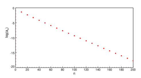
Figure 1: Logarithm of the expansion coefficients

This approach exhibits two great advantages: first, the expansion coefficients $a_{n}$ are positive so that $S_{N}<S_{N+1}$ and the sequence converges from below. Second, the expansion coefficients decrease exponentially as shown in Figure 1 and, consequently, the rate of convergence is remarkable. From the first $N\leq 5000$ partial sums we estimate

$$\varphi_{0,5000}^{\prime} = -1.58807102261137531271868450942395010945274662167482$$

$$561676567741816655196115430926233203397013842866526981$$

$$402442246654652538163078118812938288132770903659214744$$

$$086806778901475626169733142185514721772803432126893905$$

$$784750244483250437472432504160153205506367895247811586$$

$$772904901159198239550290936872919960125747115454641997$$

$$589356517736943217510752047768900396683865938312577933$$

$$839690794052221882937586$$

that is supposed to be accurate to the last digit as we carried out the calculation numerically with sufficient accuracy (a simple Python program for this purpose is available at https://zenodo.org/record/4681779#.YH2Zorh1Yqg). It is unlikely that any of the approaches applied to this problem[1, 2, 3, 4, 5, 6, 7, 9, 10, 11, 13] (and references therein) can provide a result of such an accuracy. Notice that the error of a calculation based on $S_{N}$ is roughly of the order of $a_{N+1}$.

3 Analysis of the series

In this section we will try to determine some features of the Majorana series (5) numerically. To this end we resort to a method discussed by Hunter and Guerrieri[15] some time ago that we develop in what follows in a less general and simpler way, more suitable for present needs.

The function

$$f(x)=A\left(1-\frac{x}{x_{0}}\right)^{\nu},$$ (8)

exhibits a singular point at $x=x_{0}$ for any real exponent $\nu$, except when it is a positive integer. It is sufficient for present purposes to consider $x$ real. This function can be expanded in a Taylor series

$$f(x)=\sum_{j=0}^{\infty}f_{j}x^{j},$$ (9)

that converges for all $|x|<\left|x_{0}\right|$. It follows from the differential equation

$$\left(1-\frac{x}{x_{0}}\right)f^{\prime}=-\frac{\nu}{x_{0}}f,$$ (10)

that the expansion coefficients satisfy the recurrence relation

$$(n+1)f_{n+1}=\frac{n}{x_{0}}f_{n}-\frac{\nu}{x_{0}}f_{n},\;n=0,1,\ldots.$$ (11)

We appreciate that the ratio $f_{n+1}/f_{n}$ is a linear function of $1/(n+1)$

$$\frac{f_{n+1}}{f_{n}}=\frac{1}{x_{0}}-\frac{\nu+1}{x_{0}(n+1)}.$$ (12)

From equation (11) we can derive two linear equations

$$x_{0}(n+1)f_{n+1}+\nu f_{n} = nf_{n},$$

$$x_{0}nf_{n}+\nu f_{n-1} = (n-1)f_{n-1},$$ (13)

from which we obtain

$$x_{0} = \frac{f_{n}f_{n-1}}{\left(n+1\right)f_{n+1}f_{n-1}-nf_{n}^{2}},$$

$$\nu = \frac{\left(n^{2}-1\right)f_{n+1}f_{n-1}-n^{2}f_{n}^{2}}{\left(n+1\right)f_{n+1}f_{n-1}-nf_{n}^{2}}.$$ (14)

As stated in section 2, the coefficients $a_{n}$ are all positive and decrease exponentially which suggests that $u(t)$ may exhibit a singular point as shown in equation (8). We can therefore obtain both the location $\tau_{0}$ and the exponent $\nu$ of the singular point closest to the origin from the approximate straight line

$$\frac{a_{n+1}}{a_{n}}\approx\frac{1}{\tau_{0}}-\frac{\nu+1}{\tau_{0}(n+1)},\;n\gg 1,$$ (15)

as suggested by equation (12). Alternatively, we may resort to equation (14) and estimate these parameters from

$$\tau_{0,n} = \frac{a_{n}a_{n-1}}{\left(n+1\right)a_{n+1}a_{n-1}-na_{n}^{2}},\;\tau_{0}=\lim\limits_{n\rightarrow\infty}\tau_{0,n},$$

$$\nu_{n} = \frac{\left(n^{2}-1\right)a_{n+1}a_{n-1}-n^{2}a_{n}^{2}}{\left(n+1\right)a_{n+1}a_{n-1}-na_{n}^{2}},\;\nu=\lim\limits_{n\rightarrow\infty}\nu_{n}.$$ (16)

The second and third columns of Table 1 show values of $\tau_{0,n}$ and $\nu_{n}$, respectively, obtained from equation (16) for sufficiently large values of $n$. The convergence is rather slow but it seems that $\nu_{n}$ converges towards $\nu=1/2$ from below when $n\rightarrow\infty$. The convergence of these sequences can be improved by means of of Aitken extrapolation[16] and results obtained from the last $15$ entries in the third column of table 1 confirms this conjecture. The fourth column shows results for

$$\tau_{0,n}\left(\nu=1/2\right)=\frac{n-1/2}{n+1}\frac{a_{n}}{a_{n+1}}.$$ (17)

It seems that $\tau_{0,n}\left(\nu_{n}\right)$ and $\tau_{0,n}\left(\nu=1/2\right)$ appear to be monotonously decreasing and increasing, respectively. On assuming that this behaviour already applies to all $n$ we conjecture that $1.20168605688<\tau_{0}<1.2016860577$. Straightforward application of Aitken extrapolation to the last $15$ entries in both columns enables us to sharpen those bounds to $1.2016860571<\tau_{0}<1.2016860575$. The same analysis on the third column yields $\nu=0.4998$.

On the other hand, from a numerical fit of the ratio $a_{n+1}/a_{n}$ to a straight line we estimate $\tau_{0}=1.2016860577$ and $\nu=0.4997$ in agreement with the results above.

4 Conclusions

In this paper we have shown that the Majorana transformation brought to light by Esposito[14] in a pedagogical paper enables one to obtain the slope at origin of the solution to the Thomas-Fermi equation with an accuracy that has not been achieved with any of the methods proposed so far. The slope at origin is necessary for the application of any approach because it is the relevant unknown in the nonlinear differential equation just mentioned. In addition to it, we estimated the parameters that determine the singular point closest to the origin of the function $u(t)$ appearing in the Majorana transformation of the dimensionless Thomas-Fermi equation. We conjectured that the singularity is a square-root branch point and estimated its location with reasonable precision by means of lower and upper bounds.

Table 1: Parameters for the singular point

$n$	$\tau_{0,n}(\nu_{n})$	$\nu_{n}$	$\tau_{0,n}(\nu=1/2)$
400000	1.20168605769264029435361803588	0.499705403241764669703589077642	1.20168605680760714618188774385
401000	1.20168605769043354866722488742	0.499706138707816160983219690953	1.20168605680981145947900052075
402000	1.20168605768824926820209670303	0.49970686850423206121412536936	1.20168605681199934431717238544
403000	1.2016860576860796865697237324	0.499707595193070264721085059588	1.20168605681417096352440342843
404000	1.20168605768392281024420573709	0.499708319421314682402898280176	1.20168605681632647794611242793
405000	1.20168605768178079115740801082	0.499709040445317571614381306288	1.20168605681846604642319422634
406000	1.20168605767965783307100573377	0.499709756820917562940514504979	1.20168605682058982586743506764
407000	1.2016860576775544722516936779	0.499710468331971669275852542178	1.20168605682269797125288861779
408000	1.20168605767546042850468283397	0.499711178432852468843090560012	1.20168605682479063564593371776
409000	1.20168605767338062590953642012	0.499711885437180948142052107338	1.20168605682686797024999802803
410000	1.20168605767131927381271870206	0.499712587885926043832104906147	1.20168605682893012444449010861
411000	1.20168605766927692214546468536	0.499713285557507085244966336909	1.20168605683097724578137490504
412000	1.20168605766724329181078603638	0.499713981941132448940288267412	1.20168605683300948001349255953
413000	1.20168605766522800138146309189	0.499714673721611178261717764848	1.20168605683502697114177426129
414000	1.20168605766322121156205411946	0.499715364255153566375974144531	1.20168605683702986142906660283
415000	1.20168605766123753508189521398	0.49971604848615901584789918849	1.20168605683901829144174101888
416000	1.2016860576592620129791566382	0.499716731547383522068454193635	1.20168605684099240002975438654
417000	1.20168605765730427494019569306	0.499717410088710305095020620403	1.20168605684295232439513948465
418000	1.20168605765535448415903736306	0.499718087499160887322102663134	1.2016860568448982000997565051
419000	1.20168605765342574745544322327	0.499718759200494147400208669829	1.20168605684683016110596559594
420000	1.20168605765150765389984597273	0.499719428790372125524826408218	1.2016860568487483397506528092
421000	1.20168605764960529812976599862	0.499720094468778248392634189577	1.20168605685065286682152455643
422000	1.20168605764771011681430624946	0.49972075921493538246937682624	1.2016860568525438715540418048
423000	1.20168605764583596292330946038	0.499721418145819406112338961443	1.20168605685442148167339946943
424000	1.20168605764397169184576048614	0.499722075152253704050236700056	1.20168605685628582337037319071
425000	1.20168605764212265017319322498	0.499722728329628029434508260725	1.20168605685813702137183593605
426000	1.20168605764028028246218469624	0.49972338068372267220982708216	1.20168605685997519893836744777
427000	1.20168605763845844575564932541	0.499724027284788849437199852618	1.20168605686180047790432363325
428000	1.20168605763664591943599140173	0.499724672088646643944149066554	1.20168605686361297865286240567
429000	1.20168605763484830282540948745	0.499725313083687963509247546151	1.20168605686541282018374959084
430000	1.20168605763305679932369313611	0.499725953390862034718500932713	1.20168605686720012011167472364
431000	1.20168605763128535363451068823	0.499726588003858223074707568887	1.20168605686897499470303323157
432000	1.20168605762952275020995754139	0.499727220914813576068324143944	1.20168605687073755885098422327
433000	1.20168605762777459527635201156	0.499727850091775822559729268675	1.20168605687248792614135009801
434000	1.2016860576260320960994033668	0.49972847868434786817072797909	1.20168605687422620884996548424
435000	1.20168605762430916779681415112	0.499729101651275620448833047275	1.20168605687595251797812152143
436000	1.20168605762259470597020488796	0.499729722982543095775678947105	1.20168605687766696322636321741
437000	1.20168605762089421604880153902	0.49973034066476112550458400528	1.20168605687936965305979320755
438000	1.20168605761919894526367540425	0.49973095786305836731123073029	1.20168605688106069470346942218
439000	1.2016860576175228147547327723	0.499731569488391115336882033527	1.20168605688274019417703911361
440000	1.20168605761585472407406745998	0.499732179566977791786651829719	1.2016860568844082562677809745
441000	1.20168605761420016645747662319	0.499732786072290704444252059124	1.20168605688606498459441012161

References

- [1] F. M. Fernández, Comment on: “Series solution to the Thomas-Fermi equation” [Phys. Lett. A 365 (2007) 111], Phys. Lett. A 372 (2008) 5258-5260.
- [2] S. Abbasbandy and C. Bervillier, Analytic continuation of Taylor series and the boundary value problems of some nonlinear ordinary differential equations, Appl. Math. Comput. 218 (2011) 2178-2199.
- [3] F. M. Fernández, Rational approximation to the Thomas-Fermi equations, Appl. Math. Comput. 207 (2011) 6433-6436.
- [4] J. P. Boyd, Rational Chebyshev Series for the Thomas-Fermi Function: Endpoint Singularities and Spectral Methods, J. Comp. Appl. Math. 244 (2013) 90-101.
- [5] P. Amore, J. P. Boyd, and F. M. Fernández, Accurate calculation of the solutions to the Thomas-Fermi equations, Appl. Math. Comput. 232 (2014) 929-943.
- [6] K. Parand, H. Yousefi, M. Delkhosh, and A. Ghaderi, A novel numerical technique to obtain an accurate solution to the Thomas-Fermi equation, Eur. Phys. J. Plus 131 (2016) 228.
- [7] K. Parand, A. Ghaderi, M. Delkhosh, and H. Yousefi, A new approach for solving nonlinear Thomas-Fermi equation based on fractional order rational Bessel functions, Elect. J. Diff. Eq. 2016 (2016) 1-18.
- [8] K. Parand, P. Mazaheri, and M. Delkhosh, Fractional order of rational Jacobi functions for solving the non-linear singular Thomas-Fermi equation, Eur. Phys. J. Plus 132 (2017) 77.
- [9] K. Parand and M. Delkhosh, Accurate solution of the Thomas-Fermi equation using the fractional order of rational Chebyshev functions, J. Comp. Appl. Math. 317 (2017) 624-642.
- [10] K. Parand, K. Raibei, and M. Delkhosh, An efficient numerical method for solving nonlinear Thomas-Fermi equation, Acta Univ. Sapientiae Mathematica 10 (2018) 134-151.
- [11] F. A. Parand, Z. Kalantari, M. Delkhosh, and F. Mirahmadian, A computationally hybrid Method for Solving a famous physical problem on an unbounded domain, Commun. Theor. Phys. 71 (2019) 9-15.
- [12] A. H. Hadian-Rasanan, N. Mehran, A. Bahramnezhad, M. M. Moayeri, and K. Parand, A comparison between pre-Newton and post-Newton approaches for solving a physical singular second-order boundary problem in the semi-infinite interval, arXiv:1909.04066 [math.NA]
- [13] X. Zhang and J. P. Boyd, Revisiting the Thomas-Fermi equation: accelerating rational Chebyshev series through coordinate transformations, Appl. Num. Math. 135 (2019) 186-205.
- [14] S. Esposito, Majorana solution of the Thomas-Fermi equation, Am. J. Phys. 70 (2002) 852-856.
- [15] C. Hunter and B. Guerrieri, Deducing the properties of singularities of functions from their Taylor series coefficients, SIAM J. Appl. Math. 39 (1980) 248-263.
- [16] G. Dahlquist and A Björck, Numerical Methods, Prentice-Hall, Englewood Cliffs, 1974.