Solvability of Discrete Helmholtz Equations

Abstract

We study the unique solvability of the discretized Helmholtz problem with Robin boundary conditions using a conforming Galerkin $hp$-finite element method. Well-posedness of the discrete equations is typically investigated by applying a compact perturbation argument to the continuous Helmholtz problem so that a “sufficiently rich” discretization results in a “sufficiently small” perturbation of the continuous problem and well-posedness is inherited via Fredholm’s alternative. The qualitative notion “sufficiently rich”, however, involves unknown constants and is only of asymptotic nature.

Our paper is focussed on a fully discrete approach by mimicking the tools for proving well-posedness of the continuous problem directly on the discrete level. In this way, a computable criterion is derived which certifies discrete well-posedness without relying on an asymptotic perturbation argument. By using this novel approach we obtain a) new existence and uniqueness results for the $hp$-FEM for the Helmholtz problem b) examples for meshes such that the discretization becomes unstable (stiffness matrix is singular), and c) a simple checking Algorithm MOTZ “marching-of-the-zeros” which guarantees in an a posteriori way that a given mesh is certified for a well-posed Helmholtz discretization. Helmholtz equation at high wave number; adaptive mesh generation; pre-asymptotic stability; hp-finite elements; a posteriori stability.

1 Introduction

In this paper, we consider the numerical discretization of the Helmholtz problem for modelling acoustic wave propagation in a bounded Lipschitz domain $\Omega\subset\mathbb{R}^{d}$, $d=1,2$, with boundary $\Gamma:=\partial\Omega$. Robin boundary conditions are imposed on $\Gamma$ and the strong form is given by seeking $u$ s.t.

$$\begin{array}[]{cc}-\Delta u-k^{2}u=f&\text{in }\Omega,\\ \dfrac{\partial u}{\partial\mathbf{n}}-\operatorname{i}ku=g&\text{on }\Gamma.\end{array}$$

Here, $\mathbf{n}$ denotes the outer normal vector and $k\in\mathbb{R}\backslash\left\{0\right\}$ is the wave number. It is well known that the weak formulation of this problem is well posed; the proof is based on Fredholm’s alternative in combination with the unique continuation principle (u.c.p.) (see, e.g., [Lei86]). The restriction to Robin boundary conditions is only to fix the ideas. Our method and theory apply verbatim to any other boundary condition of the type

$$\dfrac{\partial u}{\partial\mathbf{n}}-\operatorname{i}T_{k}u=g\quad\text{on }\Gamma$$

for some dissipative linear operator $T_{k}$. The generalization to mixed boundary condition which are imposed only on a subset of $\Gamma$ with positive surface measure is straightforward as well: only the initialisation of Algorithm 1 (see §4) has to be restricted to the degrees of freedom which lie on the boundary part with mixed boundary conditions.

We consider the discretization of this equation (in variational form) by a conforming Galerkin method. The proof of well-posedness for this discretization goes back to [Sch74] and is based on a perturbation argument: the subspace which defines the Galerkin discretization has to be sufficiently “rich” in the sense that a certain adjoint approximation property holds. However, this adjoint approximation property contains a constant which is a priori unknown. The existing analysis gives insights into how the parameters defining the Galerkin space should be chosen asymptotically but does not answer the question whether, for a concrete finite dimensional space, the corresponding Galerkin discretization has a unique solution.

In one spatial dimension on quasi-uniform grids the condition $kh\leq C_{\operatorname*{res}}$, for some sufficiently small minimal resolution constant $C_{\operatorname*{res}}=O\left(1\right)$, ensures unique solvability of the Galerkin discretization. This result is proved for linear finite elements on uniform meshes with $C_{\operatorname*{res}}=1$ in [IB95, Thm. 4] and for the $hp$ version of the finite element method on uniform 1D meshes with $C_{\operatorname*{res}}<\pi$ in [IB97, Thm. 3.3], i.e., on uniform grids employing $hp$ finite elements the Galerkin discretization has a unique solution if $kh\leq C_{\operatorname*{res}}<\pi$. On the other hand, piecewise linear finite elements in two or more spatial dimensions on a star-shaped domain with smooth boundary or a convex polygonal domain, a straightforward application of the Schatz’ perturbation argument leads to the much more restrictive condition: $k^{2}h\leq C_{\operatorname*{res}}\$for $C_{\operatorname*{res}}$ sufficiently small. For piecewise linear elements in spatial dimension two or three this result can be improved: if the computational domain $\Omega$ is a convex polygon/polyhedron, the condition “$k^{3}h^{2}\leq C_{\operatorname*{res}}$ for sufficiently small $C_{\operatorname*{res}}=O\left(1\right)$” ensures existence and uniqueness (see [Wu14, Thm. 6.1]). For the $hp$-finite element method on an analytically bounded or convex polygonal domain, the analysis in [MS10], [MS11] leads to the condition “$kh/p\leq C_{\operatorname*{res}}$ for $C_{\operatorname*{res}}$ sufficiently small provided the polynomial degree satisfies $p\gtrsim\log k$”.

Since no sharp bounds for the resolution constant $C_{\operatorname*{res}}$ are available for general conforming finite element meshes in 2D and 3D such estimates have merely qualitative and asymptotic character. This drawback was the motivation for the development of many novel discretization techniques by either modifying the original sesquilinear form or employing a discontinuous Galerkin discretization. Such discretizations have in common that unique solvability of the discrete problem does not rely on the Schatz argument. Unique solvability can therefore be established under less restrictive conditions; we mention [BWZ16, Wu14] for an analysis of a continuous interior penalty method with piecewise linear elements. In [Wu14, Cor. 3.5] unique solvability is established for general polygonal/polyhedral domains for any $k>0$ and $h>0$. In [FW11] interior penalty $hp$-DG methods are analysed and unique solvability for polygonal/polyhedral star-shaped domains is shown for any $k>0$ and $h>0$ under certain conditions on the penalty parameters, see [FW11, Thm 3.2] for details. Finally, in [CQ17] a least-squares approach is analysed, establishing unique solvability for domains, for which a-priori estimates of the continuous problem are available, see [CQ17, Thm 2.4].

We do not go into the details of such methods because our focus in this paper is on the question whether the conforming Galerkin discretization of the Helmholtz problem with Robin boundary conditions can lead to a system matrix which is singular and how to define a computable criterion to guarantee that for a given mesh the conforming Galerkin discretization is unique. Such an approach can be also viewed as a novel a posteriori strategy: the goal is not to improve accuracy but to guarantee unique solvability without relying on a resolution condition for a conforming Galerkin discretization.

The given finite element mesh is the input of our new algorithm called MOTZ (“marching-of-the-zeros”) which analyses the mesh, based on a stability criterion which we will develop in this paper. If the result is “certified” then the piecewise linear, conforming finite element discretization of the Helmholtz problem with Robin boundary conditions leads to a regular system matrix. Otherwise, the triangulation ist marked by MOTZ as “critical” and we will present a local mesh modification algorithm “MOTZ_flip” with the goal to obtain a modified mesh which is certified by MOTZ. In this way, MOTZ can be regarded as an a posteriori stability indicator. In contrast there exist a posteriori error estimators for the Helmholtz problem in the literature [DS13], [SZ15], [IB01], [CFEV21] which take as input a computed discrete solution and estimates the arising error in order to mark (in an ideal situation) those elements which contain the largest error contributions. However, all these error estimators are fully reliable and efficient only if a resolution condition is satisfied and the discrete system is well posed. They fail if the discrete solution does not exist and differ from our approach with respect to their goal (approximability in contrast to well-posedness). Also the adaptive algorithm in [BBHP19] is essentially of this error estimator type – however has the feature that the mesh is refined uniformly if the discrete solution does not exist. To the best of our knowledge, our approach is the first one which does not assume such conditions to hold and refines adaptively for the goal to improve stability.

The paper is organized as follows. In Section 2, we formulate the Helmholtz problem in a variational setting and recall the relevant existence and uniqueness results. Then, the conforming Galerkin discretization by $hp$-finite elements is introduced; by using a standard nodal basis the discrete problem is formulated as a matrix equation of the form $\mathbf{A}_{k}\mathbf{u}=\mathbf{r}$. Since the resulting system is finite dimensional it is sufficient to prove uniqueness of the homogeneous problem in order to get discrete solvability. We formulate this condition and obtain in a straightforward manner that the discrete homogeneous solution must vanish on the boundary $\Gamma$.

In Section 3 we discuss the invertibility of $\mathbf{A}_{k}$ for different scenarios. First, we prove in the one-dimensional case, i.e., $d=1$, that $\mathbf{A}_{k}$ is regular for any conforming $hp$-finite element space without any restrictions on the mesh size and the polynomial degree $p$. In contrast, we show in Section 3.2 that the matrix $\mathbf{A}_{k}$ can become singular for two-dimensional domains at certain discrete wave numbers for simplicial/quadrilateral meshes. We present an example of a regular triangulation of the square domain $\left(-1,1\right)^{2}$ such that the conforming piecewise linear finite element discretization of the Helmholtz problem with Robin boundary conditions leads to a singular system matrix $\mathbf{A}_{k}$. This generalizes the example in [MPS13, Ex. 3.7] where the finite element space satisfies homogeneous Dirichlet boundary conditions to the case of Robin boundary conditions. Next, we discuss conforming finite element discretizations on quadrilateral meshes and show that for rectangular domains and tensor product quadrilateral meshes the matrix $\mathbf{A}_{k}$ is always invertible for polynomial degree $p\in\left\{1,2,3\right\}$ by applying a local argument inductively. We also show that there are mesh configurations where this local argument breaks down for $p=4$.

Motivated by the results in Section 3.2, we present in Section 4 the aforementioned algorithm MOTZ. For the case that the outcome is “critical” we also present two companion algorithms which refine or modify the given mesh such that the MOTZ algorithm returns “certified”. The section is complemented by numerical experiments and a short discussion on the behaviour of the inf-sup constant before and after the modification of a “critical” mesh to a “certified” mesh.

2 Setting

Let $\Omega\subset\mathbb{R}^{d}$, $d=1,2$ be a bounded Lipschitz domain with boundary $\Gamma:=\partial\Omega$. Let $L^{2}\left(\Omega\right)$ denote the usual Lebesgue space with scalar product denoted by $\left(\cdot,\cdot\right)$ (complex conjugation is on the second argument) and norm $\|\cdot\|_{L^{2}(\Omega)}:=\left\|\cdot\right\|:=\left(\cdot,\cdot\right)^{1/2}$. Let $H^{1}\left(\Omega\right)$ denote the usual Sobolev space and let $\gamma:H^{1}\left(\Omega\right)\rightarrow H^{1/2}\left(\Gamma\right)$ be the standard trace operator. We introduce the sesquilinear forms

$$a_{0,k}\left(u,v\right):=\left(\nabla u,\nabla v\right)-k^{2}\left(u,v\right)\qquad\forall u,v\in H^{1}\left(\Omega\right)$$

and

$$b_{k}\left(u,v\right):=-\operatorname*{i}k\langle u,v\rangle_{\Gamma}\qquad\forall u,v\in H^{1/2}\left(\Gamma\right),$$

where $\langle\cdot,\cdot\rangle_{\Gamma}$ denotes the $L^{2}$ scalar product on the boundary $\Gamma$. Throughout this paper we assume that the wave number $k$ satisfies

$$k\in\overset{\circ}{\mathbb{R}}:=\mathbb{R}\backslash\left\{0\right\}\text{.}$$

The weak formulation of the Helmholtz problem with Robin boundary conditions is given as follows: For $f\in L^{2}(\Omega)$ and $g\in H^{1/2}(\Gamma)$, we define $F=(f,\cdot)+\langle g,\gamma\ \cdot\rangle_{\Gamma}\in(H^{1}\left(\Omega\right))^{\prime}$. We seek $u\in H^{1}\left(\Omega\right)$ such that

$$a_{k}\left(u,v\right):=a_{0,k}\left(u,v\right)+b_{k}\left(\gamma u,\gamma v\right)=F\left(v\right)\quad\forall v\in H^{1}\left(\Omega\right).$$ (1)

In the following, we will omit the trace operator $\gamma$ in the notation of the sesquilinear form since this is clear from the context. Well-posedness of problem (1) is proved in [Mel95, Prop. 8.1.3].

Proposition 2.1

Let $\Omega$ be a bounded Lipschitz domain. Then, (1) is uniquely solvable for all $F\in\left(H^{1}\left(\Omega\right)\right)^{\prime}$ and the solution depends continuously on the data.

We employ the conforming Galerkin finite element method for its discretization (see, e.g., [Cia78], [BS08]). For the spatial dimension, we assume that $\Omega\subset\mathbb{R}^{d}$ is an interval for $d=1$ or a polygonal domain for $d=2$. We consider either conforming meshes $\mathcal{K}_{\mathcal{T}}$ (i.e., no hanging nodes) composed of closed simplices or conforming meshes $\mathcal{K}_{\mathcal{Q}}$ composed of quadrilaterals. The set of all vertices is denoted by $\mathcal{N}$, i.e., for $\mathcal{M}\in\left\{\mathcal{T},\mathcal{Q}\right\}$

$$\mathcal{N}:=\left\{x\in\mathbb{R}^{d}~{}\mid\exists K\in\mathcal{K}_{\mathcal{M}}\text{ with }x\text{ is a vertex of }K\right\}.$$

For $d=2$, we denote the set of all edges by $\mathcal{E}$ and

$$\mathcal{E}_{\Omega}:=\left\{E\in\mathcal{E}:E\not\subset\Gamma\right\}.$$

For $p\in\mathbb{N}$, we define the continuous, piecewise polynomial finite element space by

$$\text{ for }d\in\{1,2\} S_{\mathcal{T}}^{p}:=\left\{u\in C^{0}\left(\Omega\right)\mid\forall K\in\mathcal{K}_{\mathcal{T}}:u_{|{K}}\in\mathcal{P}^{p}\right\},$$

$$\text{ for }d=2 S_{\mathcal{Q}}^{p}:=\left\{u\in C^{0}\left(\Omega\right)\mid\forall K\in\mathcal{K}_{\mathcal{Q}}:u_{|{K}}\in\mathcal{Q}^{p}\right\},$$

where $\mathcal{P}^{p}$ (resp. $\mathcal{Q}^{p}$) is the space of multivariate polynomials of maximal total degree $p$ (resp. maximal degree $p$ with respect to each variable). The reference elements are given by

$$\widehat{K}_{\mathcal{T}}:=\left\{\mathbf{x}=\left(x_{i}\right)_{i=1}^{d}\in\mathbb{R}_{\geq 0}^{d}:\sum_{i=1}^{d}x_{i}\leq 1\right\}\text{ for }d\in\{1,2\},\qquad\widehat{K}_{\mathcal{Q}}:=[-1,1]^{2}.$$

For $\mathcal{M}\in\left\{\mathcal{T},\mathcal{Q}\right\}$ and $K\in\mathcal{K}_{\mathcal{M}}$, let $\phi_{K}:\widehat{K}_{\mathcal{M}}\rightarrow K$ denote an affine pullback. Moreover for $p\geq 1$, we denote by $\hat{\Sigma}^{p}$ a set of nodal points in $\widehat{K}_{\mathcal{M}}$ unisolvent on the corresponding polynomial space which allow to impose continuity across faces. The nodal points on $K\in\mathcal{K}_{\mathcal{M}}$ are then given by lifting those of the reference element:

$$\Sigma_{K}^{p}:=\left\{\phi_{K}\left(z\right):z\in\hat{\Sigma}^{p}\right\}.$$

The set of global nodal points is given by

$$\Sigma^{p}:={\bigcup\nolimits_{K\in\mathcal{K}_{\mathcal{M}}}}\Sigma_{K}^{p},$$

and we denote by $\left(b_{z,p}\right)_{z\in\Sigma^{p}}\subset S_{\mathcal{M}}^{p}$ the standard Lagrangian basis.

Remark 2.2

For $\mathcal{M}\in\left\{\mathcal{T},\mathcal{Q}\right\}$, we write $S$ or $S_{\mathcal{M}}$ short for $S_{\mathcal{M}}^{p}$ and $\Sigma$ short for $\Sigma^{p}$ if no confusion is possible. If $p=1$ then the two sets $\mathcal{N}$ and $\Sigma^{1}$ are equal and we use the notation $\mathcal{N}$ for the set of degrees of freedom.

The Galerkin finite element method for the discretization of (1) is given by:

$$\text{find }u_{S}\in S\text{ such that }a_{k}\left(u_{S},v\right)=F\left(v\right),\quad\forall v\in S\text{.}$$ (2)

The basis representation allows us to reformulate (2) as a linear system of equations. The system matrices $\mathbf{K}=\left(\alpha_{y,z}\right)_{y,z\in\Sigma}$, $\mathbf{M}=\left(\mu_{y,z}\right)_{y,z\in\Sigma}$, $\mathbf{B}=\left(\beta_{y,z}\right)_{y,z\in\Sigma}$ are given by

$$\alpha_{y,z}:=\left(\nabla b_{z,p},\nabla b_{y,p}\right),\quad\mu_{y,z}:=\left(b_{z,p},b_{y,p}\right),\quad\beta_{y,z}:=\langle b_{z,p},b_{y,p}\rangle_{\Gamma}$$

and the right-hand side vector $\mathbf{r}=\left(\rho_{z}\right)_{z\in\Sigma}$ by $\rho_{z}=F\left(b_{z,p}\right)$. Then, the Galerkin finite element discretization leads to the following system of linear equations

$$\mathbf{A}_{k}\mathbf{u}=\mathbf{r}\quad\text{with\quad}\mathbf{A}_{k}:=\mathbf{K}-k^{2}\mathbf{M-}\operatorname*{i}k\mathbf{B},$$ (3)

where $\mathbf{u}=(u_{z})_{z\in\Sigma}$. We start off with some general remarks. It is well known that the sesquilinear form $a_{k}\left(\cdot,\cdot\right)$ satisfies a Gårding inequality and Fredholm’s alternative tells us that well-posedness of (1) follows from uniqueness. Similarly, the finite dimensional problem (2) is well posed if the problem

$$\text{find }u\in S\text{ such that }a_{k}\left(u,v\right)=0\quad\forall v\in S$$ (4)

has only the trivial solution. We note that if we choose $v=u$ and consider the imaginary part of (4), we get

$$0=\operatorname{Im}a_{k}\left(u,u\right)=-k\left\|u\right\|_{\Gamma}^{2}\implies\left.u\right|_{\Gamma}=0.$$ (5)

3 Regularity of the discrete system matrix $\mathbf{A}_{k}$

This section covers three different topics concerning the discretization of the Helmholtz equation. First, in Section 3.1 we analyse the conforming Galerkin finite element method with polynomials of degree $p\geq 1$ in spatial dimension one. Next, in Section 3.2, we present a singular two-dimensional example for piecewise linear finite elements on a triangular mesh. Finally, in Section 3.3 we consider structured tensor-product meshes in spatial dimension two.

3.1 The one-dimensional case

We prove that the conforming Galerkin finite element method for the one-dimensional Helmholtz equation is well posed for any $k\in\overset{\circ}{\mathbb{R}}$.

Theorem 3.1

Let $\Omega\subset\mathbb{R}$ be a bounded interval and consider the Galerkin discretization (2) of (1) with conforming finite elements. Then, for any $k\in\overset{\circ}{\mathbb{R}}$ the matrix $\mathbf{A}_{k}$ in (3) is regular.

Proof. We assume that $\Omega=\left(-1,1\right)$ (the result for general intervals follows by an affine transformation). Since the problem (2) is linear and finite dimensional it suffices to show that the only solution of the homogeneous problem (4) is $u=0$ . From (5) we already know that $u\left(-1\right)=u\left(1\right)=0$. We assume that the intervals $\mathcal{K}_{\mathcal{T}}=\left\{K_{i}:1\leq i\leq N\right\}$ are numbered from left to right, so that $K_{N}=\left[x_{N-1},1\right]$. The function $u_{N}:=\left.u\right|_{K_{N}}$ can be written as

$$u_{N}=\sum_{z\in\Sigma_{K_{N}}^{p}\backslash\left\{1\right\}}u_{z}b_{z,p}.$$

As test functions, we employ the functions $b_{y,p}$, $y\in\Sigma_{K_{N}}^{p}\backslash\left\{x_{N-1}\right\}$ and obtain from (4)

$$\sum_{z\in\Sigma_{K_{N}}^{p}\backslash\left\{1\right\}}\left(\alpha_{y,z}-k^{2}\mu_{y,z}\right)u_{z}=0\quad\forall y\in\Sigma_{K_{N}}^{p}\backslash\left\{x_{N-1}\right\}.$$

This is a $p\times p$ linear system and our goal is to show that it is regular for all $k\in\overset{\circ}{\mathbb{R}}$ so that $u_{z}=0$ follows for all $z\in\Sigma_{K_{N}}^{p}\backslash\left\{1\right\}$. By an affine transformation this is equivalent to the following implication

$$\forall\tilde{k}\in\overset{\circ}{\mathbb{R}}~{}\text{\textquotedblleft find }u\in\mathcal{P}_{0)}^{p}\text{ such that }\left(u^{\prime},v^{\prime}\right)-\tilde{k}^{2}\left(u,v\right)=0\quad\forall v\in\mathcal{P}_{(0}^{p}\text{\textquotedblright}\implies u=0,$$ (6)

where $\tilde{k}=2|K_{N}|k$ and

$$\mathcal{P}_{(0}^{p}:=\left\{v\in\mathcal{P}^{p}\mid v\left(-1\right)=0\right\}\quad\text{and\quad}\mathcal{P}_{0)}^{p}:=\left\{v\in\mathcal{P}^{p}\mid v\left(1\right)=0\right\}.$$

Let $u\in\mathcal{P}^{p}_{0)}$ satisfy the assumption in (6). For $\omega_{(0}\left(x\right):=1+x$ we choose $v=\omega_{(0}u^{\prime}\in\mathcal{P}^{p}_{(0}$ as a test function. We integrate by parts, use the fact $2\operatorname*{Re}(u\overline{u}^{\prime})=(|u|^{2})^{\prime}$, and employ the endpoint properties of $u$ and $v$ to obtain

$$0 =\operatorname*{Re}\left[\left(u^{\prime},\left(\omega_{(0}u^{\prime}\right)^{\prime}\right)-\tilde{k}^{2}\left(u,\omega_{(0}u^{\prime}\right)\right]$$

$$=-\operatorname*{Re}\left[\left(u^{\prime\prime},\omega_{(0}u^{\prime}\right)\right]+\left.\omega_{(0}\left|u^{\prime}\right|^{2}\right|_{-1}^{1}-\tilde{k}^{2}\left(\frac{1}{2}\left(\left|u\right|^{2}\right)^{\prime},\omega_{(0}\right)$$

$$=-\left(\frac{1}{2}\left(\left|u^{\prime}\right|^{2}\right)^{\prime},\omega_{(0}\right)+2\left|u^{\prime}\left(1\right)\right|^{2}+\frac{\tilde{k}^{2}}{2}\left\|u\right\|^{2}-\left.\frac{\tilde{k}^{2}}{2}\left|u\right|^{2}\omega_{(0}\right|_{-1}^{1}$$

$$=\frac{1}{2}\left\|u^{\prime}\right\|^{2}+\left|u^{\prime}\left(1\right)\right|^{2}+\frac{\tilde{k}^{2}}{2}\left\|u\right\|^{2}.$$

This implies that $u_{N}=\left.u\right|_{K_{N}}=0$ and we may proceed to the adjacent interval $K_{N-1}$. Since $u\left(x_{N-1}\right)=0$ we argue as before to obtain $\left.u\right|_{K_{N-1}}=0$. The result follows by induction.   

3.2 A singular example in two dimensions

In this section, we will present an example which illustrates that Robin boundary conditions are not sufficient to ensure well-posedness of the Galerkin discretization (although the continuous problem is well posed). For this, we first introduce the definition of a weakly acute angle condition on a triangulation.

Definition 3.2

Let $d=2$ and $\mathcal{T}$ a conforming triangulation of the domain $\Omega$. For an edge $E\in\mathcal{E}_{\Omega}$, we denote by $\tau_{-}$, $\tau_{+}$ the two triangles sharing $E$. Let $\alpha_{-}$ and $\alpha_{+}$ denote the angles in $\tau_{-}$, $\tau_{+}$ which are opposite to $E$. We define the angle

$$\alpha_{E}:=\alpha_{-}+\alpha_{+}.$$

We say that the edge $E$ satisfies the weakly acute angle condition if $\alpha_{E}\leq\pi$.

The following observation is key for the proof of the upcoming Lemma 3.4, as well as for the derivation of the Algorithm MOTZ (“marching-of-the-zeros”) presented in Section 4.

Lemma 3.3

Let $p=1$, i.e. $S=S^{1}_{\mathcal{T}}$. Let $E\in\mathcal{E}_{\Omega}$ be an inner edge connecting two nodes $z,z^{\prime}$. Then

$$\left(\nabla b_{z},\nabla b_{z^{\prime}}\right)\leq 0\quad\text{if and only if}\quad\alpha_{E}\leq\pi\ \text{ (i.e., }E\text{ satisfies the weakly acute angle condition)}.$$

Proof. This follows, e.g., from [Sau89, (6.8.7) Satz] (see, e.g., [SF73, p. 78] for a sufficient criterion).   

For our example, we consider $\Omega=\left(-1,1\right)^{2}$ and a mesh as depicted in Figure 1. We employ globally continuous piecewise linear finite elements, i.e., $S=S_{\mathcal{T}}^{1}$. The degrees of freedom on the boundary $\Gamma$ are located at $P_{1}^{\Gamma}=(-1,-1)^{T}$, $P_{2}^{\Gamma}=(1,-1)^{T}$, $P_{3}^{\Gamma}=(1,1)^{T}$ and $P_{4}^{\Gamma}=(-1,1)^{T}$. The inner degrees of freedom are located at $P_{1}^{\Omega}=(-\alpha,0)^{T}$, $P_{2}^{\Omega}=(0,-\alpha)^{T}$, $P_{3}^{\Omega}=(\alpha,0)^{T}$, $P_{4}^{\Omega}=(0,\alpha)^{T}$ and $P_{5}^{\Omega}=(0,0)^{T}$, with parameter $\alpha\in(0,1)$. The mesh is denoted by $\mathcal{T}_{\alpha}$. We denote the unknowns as $u_{i}^{\Gamma}$ and $u_{i}^{\Omega}$ as well as the associated basis functions with $b_{i}^{\Gamma}$ and $b_{i}^{\Omega}$ respectively.

Figure 1: Mesh resulting in a non-trivial solution of the Helmholtz equation.

Lemma 3.4

Let $\alpha\in(0,1)$ and define $k_{c}$ as

$$k_{c}=\sqrt{\frac{6(2-\alpha)}{\alpha(1-\alpha)}}.$$ (7)

Then for any $k\in\overset{\circ}{\mathbb{R}}$ the corresponding Galerkin discretization (2) of (1) with conforming piecewise linear elements on the mesh $\mathcal{T}_{\alpha}$ is well posed if $k\neq\pm k_{c}$. For $k=\pm k_{c}$ the system matrix is singular and its kernel has dimension one.

Proof. We construct an explicit non-trivial solution $u_{h}\in S_{\mathcal{T}}^{1}$ to the homogeneous equations. To that end, note that by (5) we have $u_{i}^{\Gamma}=0$ for $i=1,\dots,4$. We seek a non-trivial solution to

$$a_{0,k}(u_{h},v_{h})=(\nabla u_{h},\nabla v_{h})-k^{2}(u_{h},v_{h})=0\quad\forall v_{h}\in S_{\mathcal{T}}^{1}.$$ (8)

Our strategy is the following: We first test with the degrees of freedom associated to the boundary. This allows us to construct a candidate for a non-trivial solution. Next, we test with the interior degrees of freedom. This allows to show the existence of a critical wave number $k_{c}$ as stated in the present lemma, which can be explicitly calculated. Furthermore, we verfiy that the kernel of the system matrix for $k=\pm k_{c}$ is in fact one dimensional. Finally, we show that for any other $k\neq\pm k_{c}$ the system matrix is regular.

We test with the hat functions $b_{i}^{\Gamma}$ for $i=1,\dots,4$ associated to the degrees of freedom on the boundary in (8). Due to their support, they do not interact with the hat function $b_{5}^{\Omega}$. We start with the hat function $b_{1}^{\Gamma}$. For the construction of a candidate for a non-trivial solution, the interactions with $b_{2}^{\Gamma}$ and $b_{4}^{\Gamma}$ are redundant, since $u_{2}^{\Gamma}=u_{4}^{\Gamma}=0$. We are therefore left with the interactions with $b_{1}^{\Omega}$ and $b_{2}^{\Omega}$. Due to the weakly acute angle condition and Lemma 3.3, we find that $a_{0,k}(b_{1}^{\Gamma},b_{1}^{\Omega})<0$ for all $k\in\mathbb{R}\setminus\{0\}$. Regarding $b_{2}^{\Omega}$, we find due to the symmetry of the mesh that $a_{0,k}(b_{2}^{\Omega},b_{1}^{\Gamma})=a_{0,k}(b_{1}^{\Omega},b_{1}^{\Gamma})$. The same argument holds true for testing with the other hat functions associated to the boundary. Therefore, any solution $u_{h}$ to (8) must solve the system

$$\begin{pmatrix}\gamma&\gamma&0&0\\ 0&\gamma&\gamma&0\\ 0&0&\gamma&\gamma\\ \gamma&0&0&\gamma\end{pmatrix}\begin{pmatrix}u_{1}^{\Omega}\\ u_{2}^{\Omega}\\ u_{3}^{\Omega}\\ u_{4}^{\Omega}\end{pmatrix}=\begin{pmatrix}0\\ 0\\ 0\\ 0\end{pmatrix},$$

with $\gamma:=-a_{0,k}(b_{1}^{\Omega},b_{1}^{\Gamma})$. This system is satisfied by $(u_{1}^{\Omega},u_{2}^{\Omega},u_{3}^{\Omega},u_{4}^{\Omega})=(1,-1,1,-1)$. We now test with the hat function $b_{1}^{\Omega}$, which interacts with itself, $b_{2}^{\Omega}$ and $b_{4}^{\Omega}$ as well as $b_{5}^{\Omega}$. For some constants $a=a(\alpha)>0$ and $b=b(\alpha)>0$ we have

$$a_{0,k}(b_{1}^{\Omega},b_{1}^{\Omega})=a-k^{2}b.$$

It is easy to verify that the edge $[P_{1}^{\Omega},P_{2}^{\Omega}]$ satisfies the weakly acute angle condition for any $0<\alpha<1$. Therefore,

$$a_{0,k}(b_{2}^{\Omega},b_{1}^{\Omega})=-c-k^{2}d,$$

for some $c=c(\alpha)>0$ and $d=d(\alpha)>0$. Due to symmetry we find

$$a_{0,k}(b_{2}^{\Omega},b_{1}^{\Omega})=a_{0,k}(b_{4}^{\Omega},b_{1}^{\Omega}).$$

The same arguments hold true for the other test functions $b_{2}^{\Omega}$, $b_{3}^{\Omega}$ and $b_{4}^{\Omega}$, yielding the same values. Regarding the test function $b_{5}^{\Omega}$, the symmetry of the mesh and the satisfied weakly acute angle conditions imply

$$0>a_{0,k}(b_{i}^{\Omega},b_{5}^{\Omega})=-e\qquad\forall i=1,\dots,4$$

for some $e=e(\alpha)>0$. Furthermore, let $f:=a_{0,k}(b_{5}^{\Omega},b_{5}^{\Omega})$. The vector $(u_{1}^{\Omega},u_{2}^{\Omega},u_{3}^{\Omega},u_{4}^{\Omega},u_{5}^{\Omega})=(1,-1,1,-1,0)$ now satisfies the following system of equations:

$$\begin{pmatrix}a-k^{2}b&-c-k^{2}d&0&-c-k^{2}d&-e\\ -c-k^{2}d&a-k^{2}b&-c-k^{2}d&0&-e\\ 0&-c-k^{2}d&a-k^{2}b&-c-k^{2}d&-e\\ -c-k^{2}d&0&-c-k^{2}d&a-k^{2}b&-e\\ -e&-e&-e&-e&f\end{pmatrix}\begin{pmatrix}1\\ -1\\ 1\\ -1\\ 0\end{pmatrix}=\left(a+2c-k^{2}(b-2d)\right)\begin{pmatrix}1\\ -1\\ 1\\ -1\\ 0\end{pmatrix}.$$ (9)

Below we will show $b-2d>0$ for any $\alpha\in(0,1)$. This allows to construct exactly two solutions $k\in\mathbb{R}\setminus\{0\}$ such that $a+2c-k^{2}(b-2d)=0$, which in turn lets the right-hand side in (9) vanish so that the vector $(1,-1,1,-1,0)^{T}$ is a solution of the homogeneous equations.

To that end, let $U$ denote the upper quadrilateral with corners $P_{4}^{\Gamma}$, $P_{4}^{\Omega}$, $P_{5}^{\Omega}$, $P_{1}^{\Omega}$ and let $B$ denote the bottom quadrilateral with corners $P_{1}^{\Gamma}$, $P_{1}^{\Omega}$, $P_{5}^{\Omega}$, $P_{2}^{\Omega}$. Furthermore, let $L$ denote the left triangle with corners $P_{1}^{\Gamma}$, $P_{4}^{\Gamma}$, $P_{1}^{\Omega}$. Due to the support properties of $b_{1}^{\Omega}$ and $b_{2}^{\Omega}$ we find with the above notation that

$$b=(b_{1}^{\Omega},b_{1}^{\Omega})_{L^{2}(\Omega)}=\int_{L\cup U\cup B}(b_{1}^{\Omega})^{2}\,dx\quad\text{ and }\quad d=(b_{1}^{\Omega},b_{2}^{\Omega})_{L^{2}(\Omega)}=\int_{B}b_{1}^{\Omega}b_{2}^{\Omega}\,dx$$

Hence, we find

$$b-2d =\int_{L\cup U\cup B}(b_{1}^{\Omega})^{2}\,dx-2\int_{B}b_{1}^{\Omega}b_{2}^{\Omega}\,dx$$

$$=\int_{L}(b_{1}^{\Omega})^{2}\,dx+\int_{U}(b_{1}^{\Omega})^{2}\,dx+\int_{B}(b_{1}^{\Omega})^{2}\,dx-2\int_{B}b_{1}^{\Omega}b_{2}^{\Omega}\,dx$$

$$=\int_{L}(b_{1}^{\Omega})^{2}\,dx+\int_{U}(b_{1}^{\Omega})^{2}\,dx+\int_{B}(b_{1}^{\Omega}-b_{2}^{\Omega})^{2}\,dx-\int_{B}(b_{2}^{\Omega})^{2}\,dx$$

$$=\int_{L}(b_{1}^{\Omega})^{2}\,dx+\int_{B}(b_{1}^{\Omega}-b_{2}^{\Omega})^{2}\,dx>0,$$

where, in the last equation, we used the fact that $\int_{U}(b_{1}^{\Omega})^{2}\,dx=\int_{B}(b_{2}^{\Omega})^{2}\,dx$, which holds again due to the symmetry of the grid, which proves $b-2d>0$. In fact, tedious but elementary calculations yield that the $\alpha$ dependent quantities $a$, $c$, and $b-2d$ are given by

$$a=1+\frac{\alpha^{2}-2\alpha+2}{\alpha(2-\alpha)}+\frac{1}{1-\alpha},\qquad c=\frac{1-\alpha}{\alpha(2-\alpha)}$$

as well as

$$b-2d =\int_{L}(b_{1}^{\Omega})^{2}\,dx+\int_{B}(b_{1}^{\Omega}-b_{2}^{\Omega})^{2}\,dx$$

$$=\frac{1-\alpha}{6}+\frac{\alpha^{2}+(2-\alpha)\alpha}{12}=\frac{1}{6},$$

which yields equation (7) for the critical wave number $k_{c}$, via $a+2c-k^{2}(b-2d)=0$.

It is left to show that the vector $(1,-1,1,-1,0)^{T}$ is in fact (up to scaling) the only non-trivial solution to the homogeneous equations for $k\in\mathbb{R}\setminus\{0\}$. By the above arguments, any other candidate has to be of the form $(1,-1,1,-1,\mu)^{T}$ or $(0,0,0,0,\mu)^{T}$ for some $\mu\neq 0$.

We first show that $(0,0,0,0,\mu)^{T}$ for some $\mu\neq 0$ can never be a solution to the homogeneous equations: Assume the contrary, then similarly as in equation (9), we find $\mu(-e,-e,-e,-e,f)^{T}$ has to be the zero vector for some $\mu\neq 0$, which is impossible, since $e>0$ for any $k\in\mathbb{R}\setminus\{0\}$.

To finish the poof, we finally show that $(1,-1,1,-1,\mu)^{T}$ for some $\mu\neq 0$ can never be a solution to the homogeneous equations for $k\in\mathbb{R}\setminus\{0\}$. Again, similarly as in equation (9), we find that the following equations have to be satisfied:

$$\left(a+2c-k^{2}(b-2d)\right)\begin{pmatrix}1\\ -1\\ 1\\ -1\\ 0\end{pmatrix}+\mu\begin{pmatrix}-e\\ -e\\ -e\\ -e\\ f\end{pmatrix}=\begin{pmatrix}0\\ 0\\ 0\\ 0\\ 0\end{pmatrix}.$$

Hence, we find that $\left(a+2c-k^{2}(b-2d)\right)-\mu e=0$ (first equation) as well as $-\left(a+2c-k^{2}(b-2d)\right)-\mu e=0$ (second equation), which is only possible for $\mu=0$, since $e>0$ for any $k\in\mathbb{R}\setminus\{0\}$.   

Remark 3.5

The above example shows that there exist meshes in spatial dimension two, for which unique solvability of the discretized equations does not hold. The constructed solution has an oscillatory behaviour which can not be ruled out by the boundary hat functions. More generally, the same arguments hold true if one chooses a regular $2n$ polygon, with another rotated one inside, analogous to the above example.

Remark 3.6 (On the magnitude of the critical wave number $k$ in Lemma 3.4)

Lemma 3.4 allows to quantify the magnitude of the critical $k_{c}$ for which a non-trivial solution exists. By varying $\alpha$ in (7), the minimal $k_{c}$ is given by $k_{c}=\sqrt{6(3+2\sqrt{2})}\approx 5.91$ for the choice $\alpha=2-\sqrt{2}$. In Figure 2 (left) we visualize the behaviour of $k_{c}$ in dependence of $\alpha$. Furthermore, we present the reciprocal of the discrete inf-sup constant (see Section 4.2 for further detail) for three different values of $\alpha$, see Figure 2 (right). The singularities corresponding to the critical wave number $k_{c}$ can be observed in the plot.

Figure 2: Plot of $\alpha$ and the critical wave number $k_{c}$ (left). Plot of $k$ against the reciprocal of the discrete inf-sup constant for different values of $\alpha$ (right).

For $N\in\mathbb{N}$ consider a mesh constructed by $N^{2}$ scaled versions of the mesh considered in Lemma 3.4 as depicted in Figure 3. Let $\mathcal{T}_{\mathrm{macro}}$ denote the corresponding mesh. The mesh size $h$ is then given by $h=2N^{-1}$. A simple scaling argument together with Lemma 3.4 and Remark 3.6 allows to construct non-trivial solutions the corresponding Galerkin discretization (2) of (1) with conforming piecewise linear elements:

Figure 3: Mesh $\mathcal{T}_{\mathrm{macro}}$.

Lemma 3.7

Fix $\alpha\in(0,1)$. Let $\hat{k}_{c}$ denote the critical wave number as in equation (7). Consider a conforming Galerkin discretization (2) of (1) with piecewise linear elements on the mesh $\mathcal{T}_{\mathrm{macro}}$. Then, if $kh=2\hat{k}_{c}$ holds true, the Galerkin discretization is not uniquely solvable.

Proof. A scaling argument together with Lemma 3.4 and Remark 3.6 allows to construct a global singular solution as follows: On each of the $N^{2}$ sub-quadrilaterals one chooses the non-trivial solution constructed in the proof of Lemma 3.4. It is easy to see that with the condition $kh=2\hat{k}_{c}$ this global function is then also a non-trivial solution to the global system of homogeneous equations.   

3.3 Structured quadrilateral grids

The present section is devoted to the study of conforming Galerkin discretizations using quadrilateral elements in spatial dimension two. We employ structured tensor-product meshes. The first result concerns a $p$-version on one quadrilateral element.

Throughout this section the following notation is employed: For vectors $\mathbf{a}=\left(a_{1},a_{2}\right)$, $\mathbf{b}=\left(b_{1},b_{2}\right)$ in $\mathbb{C}^{2}$ we use the notation $\mathbf{a}\cdot\mathbf{b}:=a_{1}b_{1}+a_{2}b_{2}$ without complex conjugation. Furthermore, $\|\cdot\|_{2}$ denotes the Euclidean 2-norm.

Theorem 3.8

Let $\Omega=\widehat{K}\subset\mathbb{R}^{2}$, where $\widehat{K}$ denotes the reference quadrilateral with vertices $(\pm 1,\pm 1)^{T}$. Consider the Galerkin discretization (2) of (1) with polynomials of degree $p\geq 1$ on $\widehat{K}$. Then, for any $k\in\overset{\circ}{\mathbb{R}}$ the matrix $\mathbf{A}_{k}$ in (3) is regular.

Proof. As in the proof of Theorem 3.1 it suffices to show that any solution for the homogeneous problem is already trivial. Throughout the proof, we denote by $S$ the finite element space, i.e., the space of polynomials of total degree $p$ on $\widehat{K}$. Let $u\in S$ be a solution to the homogeneous equations. We again have $u=0$ on $\partial\widehat{K}$, see equation (5). Therefore, $u\in S$ solves

$$(\nabla u,\nabla v)-k^{2}(u,v)=0\quad\forall v\in S.$$ (10)

The proof relies, similarly to Theorem 3.1, on the choice of a special kind of test functions, i.e. Morawetz-multipliers. Note that for any $a$, $b$, $c$, $d\in\mathbb{R}$ we have $(ax+b)u_{x}\in S$ and $(cy+d)u_{y}\in S$. Therefore, with $\boldsymbol{\rho}:=(ax+b,cy+d)^{T}$ the function $v=\boldsymbol{\rho}\cdot\nabla u\in S$ is a valid test function. Choosing $v=\boldsymbol{\rho}\cdot\nabla u$ in (10), passing to the real part, integrating by parts together with the facts that $2\operatorname*{Re}(w\overline{w}_{x})=\partial_{x}(|w|^{2})$ and $2\operatorname*{Re}(w\overline{w}_{y})=\partial_{y}(|w|^{2})$ for sufficiently smooth functions $w$ and employing the boundary conditions of $u$, we find

$$0 =\operatorname*{Re}\,\left[(\nabla u,\nabla(\boldsymbol{\rho}\cdot\nabla u))-k^{2}(u,\boldsymbol{\rho}\cdot\nabla u)\right]$$

$$=\operatorname*{Re}\,\left[(\nabla u,\nabla\boldsymbol{\rho}\,\nabla u)+(\nabla u,\nabla^{2}u\,\boldsymbol{\rho})-k^{2}(u,\boldsymbol{\rho}\cdot\nabla u)\right]$$

$$=\operatorname*{Re}\,\left[(\nabla u,\nabla\boldsymbol{\rho}\,\nabla u)\right]+\frac{1}{2}(\nabla\lVert\nabla u\rVert_{2}^{2},\boldsymbol{\rho})-\frac{k^{2}}{2}(\nabla|u|^{2},\boldsymbol{\rho})$$

$$=\operatorname*{Re}\,\left[(\nabla u,\nabla\boldsymbol{\rho}\,\nabla u)\right]-\frac{1}{2}(\lVert\nabla u\rVert_{2}^{2},\nabla\cdot\boldsymbol{\rho})+\frac{1}{2}\langle\lVert\nabla u\rVert_{2}^{2},\boldsymbol{\rho}\cdot\mathbf{n}\rangle+\frac{k^{2}}{2}(|u|^{2},\nabla\cdot\boldsymbol{\rho})-\underbrace{\frac{k^{2}}{2}\langle|u|^{2},\boldsymbol{\rho}\cdot\mathbf{n}\rangle}_{=0}.$$

The choice $\boldsymbol{\rho}=(1-x,1-y)^{T}$, results in $\nabla\boldsymbol{\rho}-1/2\,\nabla\cdot\boldsymbol{\rho}\,I$ being the zero matrix. Furthermore, $\nabla\cdot\boldsymbol{\rho}=-2$. We therefore have

$$\frac{1}{2}\langle\lVert\nabla u\rVert_{2}^{2},\boldsymbol{\rho}\cdot\mathbf{n}\rangle-k^{2}\lVert u\rVert_{L^{2}(\widehat{K})}^{2}=0.$$

We find $u\equiv 0$ once we have shown $\boldsymbol{\rho}\cdot\mathbf{n}\leq 0$. Since $\boldsymbol{\rho}\cdot\mathbf{n}=0$ on the top-right part of $\partial\widehat{K}$ and $\boldsymbol{\rho}\cdot\mathbf{n}=-2$ on the bottom-left part, we can conclude $u\equiv 0$.   

The natural next step is to consider an axial parallel quadrilateral domain $\Omega\subset\mathbb{R}^{2}$ and use a mesh, which consists of one corridor of elements, see Figure 4.

Figure 4: Example of a mesh as in Theorem 3.9.

Theorem 3.9

Let $\Omega\subset\mathbb{R}^{2}$ be an axial parallel quadrilateral. Consider the Galerkin discretization (2) of (1) with conforming finite elements with a mesh consisting of a corridor of axial parallel quadrilaterals as depicted in Figure 4 and polynomial degree $p\geq 1$. Then, for any $k\in\overset{\circ}{\mathbb{R}}$ the matrix $\mathbf{A}_{k}$ in (3) is regular.

Proof. Without loss of generality, we may assume that two of the sides of $\Omega$ are on the lines $\{y=1\}$ and $\{y=-1\}$. Choosing $v=u$ and passing to the imaginary part again leads to $u=0$ on $\Gamma$. We also find

$$0=(\lVert\nabla u\rVert_{2}^{2},1)-k^{2}(|u|^{2},1).$$ (11)

Due to the axial symmetric mesh, the function $(1-y)u_{y}$ is a valid test function. We can also write $(1-y)u_{y}=\boldsymbol{\rho}\cdot\nabla u$ with $\boldsymbol{\rho}=(0,1-y)^{T}$. Proceeding as in the proof of Theorem 3.8 we find

$$0 =\operatorname*{Re}\,\left[(\nabla u,\nabla(\boldsymbol{\rho}\cdot\nabla u))-k^{2}(u,\boldsymbol{\rho}\cdot\nabla u)\right]$$

$$=(\nabla u,\nabla\boldsymbol{\rho}\,\nabla u)-\frac{1}{2}(\lVert\nabla u\rVert_{2}^{2},\nabla\cdot\boldsymbol{\rho})+\frac{1}{2}\langle\lVert\nabla u\rVert_{2}^{2},\boldsymbol{\rho}\cdot\mathbf{n}\rangle+\frac{k^{2}}{2}(|u|^{2},\nabla\cdot\boldsymbol{\rho})-\frac{k^{2}}{2}\langle|u|^{2},\boldsymbol{\rho}\cdot\mathbf{n}\rangle.$$

Again we find $\langle|u|^{2},\boldsymbol{\rho}\cdot\mathbf{n}\rangle=0$. Furthermore, note that

$$\nabla\boldsymbol{\rho}=\begin{pmatrix}0&0\\ 0&-1\end{pmatrix}\qquad\text{ and }\qquad\nabla\cdot\boldsymbol{\rho}=-1.$$

Finally $\boldsymbol{\rho}\cdot\mathbf{n}=-2$ on the line $\{y=-1\}$ and vanishes on all other sides of the boundary. Therefore, the above further simplifies to

$$0=\frac{1}{2}(|u_{x}|^{2},1)-\frac{1}{2}(|u_{y}|^{2},1)-\langle|u_{y}|^{2},1\rangle_{\{y=-1\}}-\frac{k^{2}}{2}(|u|^{2},1).$$ (12)

Multiplying (11) by $-1/2$ and adding (12) leads to

$$0=-(|u_{y}|^{2},1)-\langle|u_{y}|^{2},1\rangle_{\{y=-1\}}.$$

Consequently, $u_{y}\equiv 0$. Combined with the fact that $u$ vanishes on the boundary we find $u\equiv 0$, which concludes the proof.   

Figure 5: Example of a mesh as in Theorem 3.10.

Theorem 3.10

Let $\Omega\subset\mathbb{R}^{2}$ be an axial parallel quadrilateral. Consider the Galerkin discretization (2) of (1) with conforming finite elements with a mesh consisting of two corridors of axial parallel quadrilaterals as depicted in Figure 5. Then, for any $k\in\overset{\circ}{\mathbb{R}}$ the matrix $\mathbf{A}_{k}$ in (3) is regular.

Proof. Without loss of generality, we may assume that the dividing line between the two corridors to be located on the line $\{y=0\}$. Let the two sides parallel to the $x$-axis lie on the lines $\{y=a\}$ and $\{y=-b\}$, for some $a$, $b>0$. Let $U\subset\Omega$ and $D\subset\Omega$ denote the upper and lower corridor respectively. Again the proof relies on an appropriate choice of test functions. These are the global function $v=u$, as well as $v=-2yu_{y}$ localized on $U$ and $D$ respectively, i.e., extended by zero. This localization is again a valid test function since $v=-2yu_{y}$ is piecewise polynomial and conforming since $v=0$ on the line $\{y=0\}$. Analogous integration by parts as in the proof of Theorem 3.10 we find the following three equations to hold:

$$0 =(|u_{x}|^{2},1)_{\Omega}+(|u_{y}|^{2},1)_{\Omega}-k^{2}(|u|^{2},1)_{\Omega},$$

$$0 =(|u_{x}|^{2},1)_{U}-(|u_{y}|^{2},1)_{U}-\langle|u_{y}|^{2},1\rangle_{\{y=a\}}-k^{2}(|u|^{2},1)_{U},$$

$$0 =(|u_{x}|^{2},1)_{D}-(|u_{y}|^{2},1)_{D}-\langle|u_{y}|^{2},1\rangle_{\{y=-b\}}-k^{2}(|u|^{2},1)_{D}.$$

Adding the equations for $U$ and $D$ and subtracting the one on the whole domain $\Omega$ again gives $u_{y}\equiv 0$, which concludes the proof, with the same arguments as in the proof of Theorem 3.9.   

The previous results relied on the use of appropriate global test functions. The remainder of this section is concerned with discretizations employing quadrilaterals on structured Cartesian meshes. To that end let $\widehat{K}$ again denote the reference quadrilateral with vertices $(\pm 1,\pm 1)^{T}$. The setup is such that the bottom-left part of the boundary of $\widehat{K}$ is part of the boundary $\Gamma$ of the computational domain $\Omega$, again itself an axial parallel quadrilateral. The upper right part of the boundary of $\widehat{K}$ is therefore inside the domain $\Omega$. Our argument will be a localized one, i.e., we consider only test functions $v$ whose support is given by $\widehat{K}$. To that end let $\mathcal{Q}_{\mathrm{BL}}^{p}(\widehat{K})$ denote that space of polynomials of total degree $p$, which are zero on the bottom-left part of the boundary of $\widehat{K}$. Analogously let $\mathcal{Q}_{\mathrm{TR}}^{p}(\widehat{K})$ denote that space of polynomials of total degree $p$, which are zero on the top-right part of the boundary of $\widehat{K}$. These spaces are therefore given by

$$\mathcal{Q}_{\mathrm{BL}}^{p}(\widehat{K}) =\mathrm{span}\left\{(1+x)(1+y)x^{i}y^{j}\colon 0\leq i,j\leq p-1\right\},$$

$$\mathcal{Q}_{\mathrm{TR}}^{p}(\widehat{K}) =\mathrm{span}\left\{(1-x)(1-y)x^{i}y^{j}\colon 0\leq i,j\leq p-1\right\}.$$

To perform a localized argument, we only test with functions $v\in\mathcal{Q}_{\mathrm{TR}}^{p}(\widehat{K})$. Note that the Galerkin solution $u$ vanishes on the bottom-left part of the boundary of $\widehat{K}$ and therefore $\left.u\right|_{\widehat{K}}\in\mathcal{Q}_{\mathrm{BL}}^{p}(\widehat{K})$. These considerations now lead to the question if a solution $u\in\mathcal{Q}_{\mathrm{BL}}^{p}(\widehat{K})$ of

$$(\nabla u,\nabla v)_{\widehat{K}}-k^{2}(u,v)_{\widehat{K}}=0\qquad\forall v\in\mathcal{Q}_{\mathrm{TR}}^{p}(\widehat{K})$$ (13)

can only be $u\equiv 0$. Upon introducing $b_{\mathrm{i}}=(1+x)(1+y)$ and $b_{\mathrm{o}}(x,y)=(1-x)(1-y)$, we can write $u=b_{\mathrm{i}}u_{r}$ and $v=b_{\mathrm{o}}v_{r}$ for polynomials $u_{r}$, $v_{r}\in\mathcal{Q}^{p-1}(\widehat{K}):=\mathrm{span}\left\{x^{i}y^{j}\colon 0\leq i,j\leq p-1\right\}$. The above is therefore equivalent to whether a solution $u_{r}\in\mathcal{Q}^{p-1}(\widehat{K})$ to

$$(\nabla(b_{\mathrm{i}}u_{r}),\nabla(b_{\mathrm{o}}v_{r}))_{\widehat{K}}-k^{2}(b_{\mathrm{i}}u_{r},b_{\mathrm{o}}v_{r})_{\widehat{K}}=0\qquad\forall v_{r}\in\mathcal{Q}^{p-1}(\widehat{K})$$ (14)

can only be $u_{r}\equiv 0$. The answer to this question is yes for $p=1$, $2$, $3$. However, for $p=4$ and some $k>0$ such exists a non-trivial solution. The consequences of this are twofold: Firstly, on a structured Cartesian grid, the Galerkin discretizations for $p=1$, $2$, $3$ are well posed for any $k\in\mathbb{R}\backslash\left\{0\right\}$. Secondly, for $p\geq 4$ a localized argument based on the appropriate choice of test functions as in the one-dimensional case, see Theorem 3.1, is not possible in two dimensions, for all wave numbers simultaneously.

Lemma 3.11

For $p=1$, $2$, $3$ the only solution to (14) is the trivial solution $u_{r}\equiv 0$, for every $k\in\overset{\circ}{\mathbb{R}}$. For $p=4$ and some $k>0$ there exists a non-trivial solution to (14).

Proof. The proof is an algebraic one. We calculate the matrix corresponding to the system of linear equations (14) explicitly. To that end we choose the monomial basis of $\mathcal{Q}^{p-1}(\widehat{K})$, i.e., for $p=1$ the basis is given by $\{1\}$, for $p=2$ by $\{1,y,x,xy\}$ and for $p=3$ by $\{1,y,y^{2},x,xy,xy^{2},x^{2},x^{2}y,x^{2}y^{2}\}$. For $p=1$, i.e., a $1\times 1$ system, we find for the determinant the polynomial

$$-\frac{16}{3}-k^{2}\frac{16}{9},$$

which is strictly negative for any $k\in\mathbb{R}$. For $p=2$ we find

$$\mathrm{det}\left(\begin{pmatrix}-\frac{16}{3}&\frac{8}{3}&\frac{8}{3}&0\\[6.0pt] -\frac{8}{3}&-\frac{64}{45}&0&\frac{8}{15}\\[6.0pt] -\frac{8}{3}&0&-\frac{64}{45}&\frac{8}{15}\\[6.0pt] 0&-\frac{8}{15}&-\frac{8}{15}&-\frac{16}{45}\\ &&&\end{pmatrix}-k^{2}\begin{pmatrix}\frac{16}{9}&0&0&0\\[6.0pt] 0&\frac{16}{45}&0&0\\[6.0pt] 0&0&\frac{16}{45}&0\\[6.0pt] 0&0&0&\frac{16}{225}\\ &&&\end{pmatrix}\right)=\frac{65536\left(k^{2}+4\right)^{2}\left(k^{4}+8k^{2}+60\right)}{4100625},$$

which is again non-zero. For $p=3$ we find the determinant is given, up to a positive factor, by

$$-\left(k^{6}+15k^{4}+270k^{2}+3150\right)\left(4k^{6}+60k^{4}+495k^{2}+450\right)^{2}.$$

For $p=4$ we find the following polynomial to be a factor of the determinant

$$(-3492720-161028k^{2}+41013k^{4}+10800k^{6}+810k^{8}+36k^{10}+k^{12})^{2},$$

which has a positive real root.   

An immediate consequence of Lemma 3.11 is the following Theorem.

Theorem 3.12

Let $\Omega\subset\mathbb{R}^{2}$ be an axial parallel quadrilateral. Consider the Galerkin discretization (2) of (1) with conforming finite elements with a tensor-product mesh and polynomial degree $p=1$, $2$, $3$. Then, for any $k\in\overset{\circ}{\mathbb{R}}$ the matrix $\mathbf{A}_{k}$ in (3) is regular.

Proof. Propagating through the mesh by applying Lemma 3.11 yields the result.   

4 A discrete unique continuation principle for the Helmholtz equation

In this section, we will introduce the Algorithm MOTZ (“marching-of-the-zeros”), which mimics a discrete unique continuation principle for the Helmholtz equation for $d=2$ and a triangular mesh $\mathcal{K}_{\mathcal{T}}$. We restrict ourselves to the case where $p=1$ and use the notation as in Remark 2.2. The discrete problem then reads

$$\text{find }u_{S}\in S\text{ such that }a_{k}\left(u_{S},v\right)=F\left(v\right),\quad\forall v\in S,$$ (15)

where $S=S^{1}_{\mathcal{T}}$ is the space of continuous and piecewise linear functions with respect to a conforming triangulation $\mathcal{K}_{\mathcal{T}}$ on $\Omega$.

Notation 4.1

In the following, we skip the polynomial degree $p$ in the notation and write short $b_{z}$ for $b_{z,p}=b_{z,1}$.

Definition 4.2

Let $\mathcal{N}_{1}\subset\mathcal{N}$ be a subset of nodes. For a node $z^{\prime}\in\mathcal{N}_{1}$ we define the transmission degree with respect to $\mathcal{N}$ by

$$\mathrm{deg}(z^{\prime},\mathcal{N}_{1})=\operatorname*{card}\left\{z\in\mathcal{N}\setminus\mathcal{N}_{1}\mid[z,z^{\prime}]\in\mathcal{E}_{\Omega}\right\}.$$

Lemma 4.3

Let $d=2$ and $\mathcal{N}_{\operatorname*{test}}\subset\mathcal{N}$ a subset of nodes. Let $z\in\mathcal{N}_{\operatorname*{dof}}:=\mathcal{N}\setminus\mathcal{N}_{\operatorname*{test}}$ have the property: there exists $z^{\prime}\in\mathcal{N}_{\operatorname*{test}}$ with

1. $E=[z,z^{\prime}]\in\mathcal{E}_{\Omega}$ and $\alpha_{E}\leq\pi$,

2. $\deg(z^{\prime},\mathcal{N}_{\operatorname*{test}})=1$,

(see Figure 6). Let $u\in S$ be a solution of (15). Then the following implication holds

$$u(z^{\prime\prime})=0~{}~{}\forall z^{\prime\prime}\in\mathcal{N}_{\operatorname*{test}}\implies u(z)=0.$$ (16)

Figure 6: The setting for Lemma 4.3
( $\in\mathcal{N}_{\operatorname{test}}$ and $\in\mathcal{N}_{\operatorname{dof}}$ ).

Notation 4.4

We generally denote by $\mathcal{N}_{\operatorname*{test}}\subset\mathcal{N}$ a subset of nodes $z$, where we already know that the solution $u$ of (15) is zero, i.e., $u_{z}=0$ as in the assumption in (16), but where we have a basis function $b_{z}$ that can be used as test function. An example is $\mathcal{N}_{\operatorname*{test}}=\mathcal{N}\cap\Gamma$. Indeed, from (5), we know that $u_{z}=0\$for all $z\in\mathcal{N}\cap\Gamma$.

Remark 4.5

If the weakly acute angle condition

$$\alpha_{E}\leq\pi$$ (17)

is violated for some edge $E\in\mathcal{E}_{\Omega}$ one can take the midpoint of $E$ as a new mesh point and bisect the adjacent triangles. For general dimension $d$, an analogous angle criterion as (17) can be formulated (see [XZ99, Lem. 2.1]).

Proof of Lemma 4.3. Let $b_{z^{\prime}}$ be the Lagrange basis function for the node $z^{\prime}$ and $b_{z}$ the one for $z$. Then (16) is equivalent to showing

$$\left(\nabla b_{z},\nabla b_{z^{\prime}}\right)-k^{2}\left(b_{z},b_{z^{\prime}}\right)\neq 0.$$ (18)

By Lemma 3.3 we have that $\left(\nabla b_{z},\nabla b_{z^{\prime}}\right)\leq 0$ if and only if $\alpha_{E}\leq\pi$. Since $b_{z}$ and $b_{z^{\prime}}$ are positive in $\operatorname*{int}\left(\tau_{+}\right)\cup\operatorname{int}\left(\tau_{-}\right)$, we conclude that (18) holds.   

4.1 A first checking algorithm and numerical experiments

In this section we present a main result of the paper (cf. Theorem 4.8): If the algorithm MOTZ (Algorithm 1) returns certified then we conclude that the discrete problem is well posed. On the other hand, if the output is critical then this means that the discretization might lead to a singular matrix. In the latter case a slight modification of the mesh (using bisection or flip of an edge) may be applied to receive a regular system matrix. We introduce the following notation

• $\mathcal{N}_{\operatorname*{test}}$: The set of $z\in\mathcal{N}$ where $u(z)=0$.

• $\mathcal{N}_{\operatorname*{dof}}$: The complement of $\mathcal{N}_{\operatorname*{test}}$.

		$\xrightarrow[\shortstack{${\color[rgb]{0,0,0}\mathcal{N}_{\operatorname{dof}}}={\color[rgb]{0,0,0}\mathcal{N}_{\operatorname{dof}}}\setminus\{z\}$}]{\shortstack{ ${\color[rgb]{0,0,0}\mathcal{N}_{\operatorname{test}}}={\color[rgb]{0,0,0}\mathcal{N}_{\operatorname{test}}}\cup\{z\}$ }}$
$\xrightarrow{\phantom{loooong}}$		$\xrightarrow[\shortstack{${\color[rgb]{0,0,0}\mathcal{N}_{\operatorname{dof}}}={\color[rgb]{0,0,0}\mathcal{N}_{\operatorname{dof}}}\setminus\{z\}$}]{\shortstack{ ${\color[rgb]{0,0,0}\mathcal{N}_{\operatorname{test}}}={\color[rgb]{0,0,0}\mathcal{N}_{\operatorname{test}}}\cup\{z\}$ }}$

Figure 7: Procedure described in Alg. 1 ( $\in\mathcal{N}_{\operatorname{test}}$ and $\in\mathcal{N}_{\operatorname{dof}}$ ).

The idea of Algorithm 1 is the following: We initialize the algorithm with $\mathcal{N}_{\operatorname*{test}}=\mathcal{N}\cap\Gamma$ and $\mathcal{N}_{\operatorname*{dof}}=\mathcal{N}\setminus\mathcal{N}_{\operatorname*{test}}$. Recall that for $z^{\prime}\in\mathcal{N}_{\operatorname*{test}}$ with $\deg\left(z^{\prime},\mathcal{N}_{\operatorname*{test}}\right)=1$ (cf. Definition 4.2) there exists one and only one $z^{\prime}\in\mathcal{N}_{\operatorname*{dof}}$ such that the edge $E=\left[z,z^{\prime}\right]$ belongs to $\mathcal{E}_{\Omega}$. Lemma 4.3, together with (5) then implies that $u(z)=0$. We update the sets $\mathcal{N}_{\operatorname*{test}}=\mathcal{N}_{\operatorname*{test}}\cup\{z\}$ and $\mathcal{N}_{\operatorname*{dof}}=\mathcal{N}_{\operatorname*{dof}}\setminus\{z\}$ accordingly and repeat the same procedure. After each step one has

$$u(z^{\prime\prime})=0~{}~{}\forall z^{\prime\prime}\in\mathcal{N}_{\operatorname*{test}}.$$

If $\mathcal{N}_{\operatorname*{test}}=\mathcal{N}$ the algorithm stops.

We remark that we do not stop the algorithm if the weakly acute angle condition (17) is not satisfied. Instead, we assign to the corresponding edge the property acute(E) = false (line 7 of Alg. 1). If angle conditions are not satisfied everywhere, but the algorithm ends with $\mathcal{N}_{\operatorname{test}}=\mathcal{N}$, we bisect the relevant, adjacent triangles in a post-processing step as explained in Remark 4.5 using Algorithm 2 in the end. This is possible since two transmission edges never share an adjacent triangle.

Algorithm 1 MOTZ

Input: $\mathcal{N}_{\operatorname{test}}$, $\mathcal{N}$, $\mathcal{E}_{\Omega}$
    Output: MOTZ_result, MOTZ_trans, MOTZ_angle, $\mathcal{N}_{\operatorname{test}}$, $\mathcal{N}_{\operatorname{dof}}$, $\mathcal{E}_{\Omega}$

1:  MOTZ_result = certified, MOTZ_trans = true, MOTZ_angle = true

2:  $\mathcal{N}_{\operatorname{dof}}:=\mathcal{N}\setminus\mathcal{N}_{\operatorname{test}}$

3:  while $\mathcal{N}_{\operatorname{dof}}\neq\emptyset$ do

4:     if $\exists(z,z^{\prime})\in\mathcal{N}_{\operatorname{dof}}\times\mathcal{N}_{\operatorname{test}}$: $E=[z,z^{\prime}]\in\mathcal{E}_{\Omega}$ $\wedge$ $\deg(z^{\prime},\mathcal{N}_{\operatorname{test}})=1$ then

5:        trans$(E)=\textbf{true}{}$

6:        if $\alpha_{E}>\pi$ then

7:           acute$(E)=\textbf{false}{}$

8:           MOTZ_angle = false

9:        end if

10:        $\mathcal{N}_{\operatorname{test}}=\mathcal{N}_{\operatorname{test}}\cup\{z\}$

11:        $\mathcal{N}_{\operatorname{dof}}=\mathcal{N}_{\operatorname{dof}}\setminus\{z\}$

12:     else

13:        MOTZ_trans = false ; STOP

14:     end if

15:  end while

16:  if MOTZ_angle == false $\vee$ MOTZ_trans == false then

17:     MOTZ_result = critical

18:  end if

Algorithm 2 correct_angle_condition

Input: $\mathcal{N}$, $\mathcal{E}_{\Omega}$
    Output: updated $\mathcal{N}$, $\mathcal{E}_{\Omega}$

1:  for all $E\in\mathcal{E}_{\Omega}$ with $\operatorname{trans}(E)=\textbf{true}{}$ $\wedge$ $\alpha_{E}>\pi$ do

2:     bisect $E$ until weakly acute angle condition is satisfied

3:  end for

Lemma 4.6

After a finite number of bisections the weakly acute angle condition is satisfied.

Proof. We consider the setting depicted in Figure 9. Let $\tau=[A,B,C]$ be a triangle with corresponding angles $\alpha,\beta,\gamma$ such that $\alpha\leq\beta<\gamma$ and $\gamma>\frac{\pi}{2}$. After one bisection the angle $\gamma$ splits in two angles $\gamma_{1}+\gamma_{2}=\gamma$ (cf. Figure 9) with the convention $\gamma_{1}\leq\gamma_{2}$. Then $\gamma_{1}\geq\alpha$ [SEP98, Eq. (4) and (6)]. This implies that $\gamma_{1}\leq\gamma_{2}=\gamma-\gamma_{1}\leq\gamma-\alpha$. If $\gamma_{2}>\frac{\pi}{2}$, then another bisection implies with the same arguments that $\gamma_{3},\gamma_{4}\leq\gamma-2\alpha$, since $\beta\geq\alpha$ as well as $\tilde{\alpha}=\alpha+\alpha_{1}\geq\alpha$. We conclude that after a finite number $n$ of bisections (depending on the smallest angle in the triangle), all angles $\gamma_{i}$, which subdivide $\gamma$, i.e., $\sum_{i=1}^{n+1}\gamma_{i}=\gamma$ satisfy $\gamma_{i}\leq\frac{\pi}{2}$.   

Figure 8: Setting for Lemma 4.6.

Figure 9: The setting for Lemma 4.7.
( $\in\mathcal{N}_{\operatorname{test}}$, $\in\mathcal{N}_{\operatorname{dof}}$).

Lemma 4.7

Assume that the Algorithm MOTZ returns MOTZ_angle = false and MOTZ_trans = true for a given Galerkin discretization as in (15). Running the bisection Algorithm 2, does not change the outcome of MOTZ_trans.

Proof. Let $E=[z^{\prime},z]$ be a transmission edge such that $\alpha_{E}>\pi$. After one bisection of $E$, a new vertex $\tilde{z}$ on $E$ is added (cf. Figure 9). In order to have the same outcome of Algorithm MOTZ_trans we need to show that $u(z^{\prime})=u(z)=0$. Indeed, this follows from applying Lemma 4.3 along the edge $[z^{\prime},\tilde{z}]$ and then $[\tilde{z},z]$, provided the angle condition is met. If the angle condition does not hold, the argument can be repeated for every subsequent bisection. The algorithm stops after a finite number of bisections, according to Lemma 4.6.   

Theorem 4.8

Consider the Galerkin discretization of (1) by (15).

1. If MOTZ$(\mathcal{N}\cap\Gamma,\mathcal{N},\mathcal{E}_{\Omega})$ returns the value MOTZ_result = certified, then the system matrix $\mathbf{A}_{k}$ in (3) is regular for any $k\in\overset{\circ}{\mathbb{R}}$.

2. If MOTZ$(\mathcal{N}\cap\Gamma,\mathcal{N},\mathcal{E}_{\Omega})$ returns the values MOTZ_trans = true and MOTZ_angle = false, then after running Algorithm 2, the system matrix $\mathbf{A}_{k}$ in (3) for the new mesh is regular any $k\in\overset{\circ}{\mathbb{R}}$.

Proof. From $u\in S$ and (5) we know that $\left.u\right|_{\Gamma}=0$. Choose $z_{1}$, $z_{1}^{\prime}$ as defined in Algorithm 1 MOTZ and set $E=\left[z_{1},z_{1}^{\prime}\right]$. With Lemma 4.3, we conclude that $u\left(z_{1}^{\prime}\right)=0$. By an inductive application of this argument to pairs ($z_{j}$, $z_{j}^{\prime}$) we obtain that $u$ is zero at all $z\in\mathcal{N}$. This means that $u$ vanishes in all mesh points $\mathcal{N}$. If MOTZ_trans = true, but MOTZ_angle = false, running Algorithm 2 makes sure that for the new mesh all relevant weakly acute angle conditions are met. This procedure does not change the output of MOTZ_trans as proved in Lemma 4.7. Therefore, if we run Algorithm 1 with the new mesh the output will be MOTZ_result = certified and the first statement of the theorem applies.   

Remark 4.9

In general, a lower bound on the smallest angle of the mesh determines how many bisections are at most needed. In all examples that are presented in this publication, all weakly acute angle conditions were satisfied. In particular this means that the outcome MOTZ_result solely depended on the outcome MOTZ_trans, i.e. on the connectivity of the mesh. We also note that the algorithm could easily be modified in order to avoid edges which do not satisfy the weakly acute angle conditions (if possible). However, since acute angle conditions in our examples were always met, this was not implemented in our code.

Figure 10(a) shows the finite element mesh of a non-convex geometry with re-entrant corners. The boundary with Robin boundary conditions is illustrated in blue. In order to determine if the Galerkin finite element method (15) for this mesh is well posed, we apply Algorithm 1 with $\mathcal{N}_{\operatorname*{test}}$ being the nodes on the boundary (cf. Figure 10(b)). The red nodes belong to $\mathcal{N}_{\operatorname*{dof}}$.
In the subsequent figures the evolution of the algorithm is shown. It successively tries to find nodes in $\mathcal{N}_{\operatorname*{dof}}$ that have a neighbouring node in $\mathcal{N}_{\operatorname*{test}}$ with transmission degree 1. Once such a node has been identified, it is removed from $\mathcal{N}_{\operatorname*{dof}}$ and added to $\mathcal{N}_{\operatorname*{test}}$. In this example the procedure can be repeated until $\mathcal{N}_{\operatorname*{dof}}$ is the empty set and $\mathcal{N}_{\operatorname*{test}}=\mathcal{N}$, i.e., MOTZ will return MOTZ_trans = true. Since also all angle conditions are satisfied the algorithm will return certified. Furthermore, due to the regularity of the mesh, nodes that satisfy condition (a) of Lemma 4.3 are easily found in each step, since they are typically located next to the node that has been removed from $\mathcal{N}_{\operatorname*{dof}}$ in the previous step.
Note that the order in which nodes are removed from $\mathcal{N}_{\operatorname*{dof}}$ depends on the enumeration of the nodes in the mesh. The outcome MOTZ_trans however, is independent of the node enumeration.

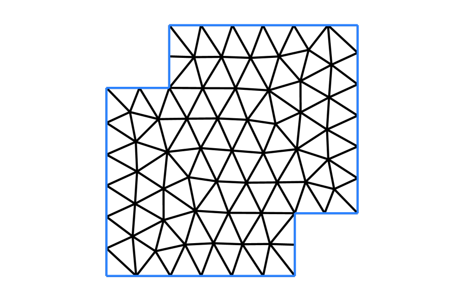
(a) Mesh with boundary

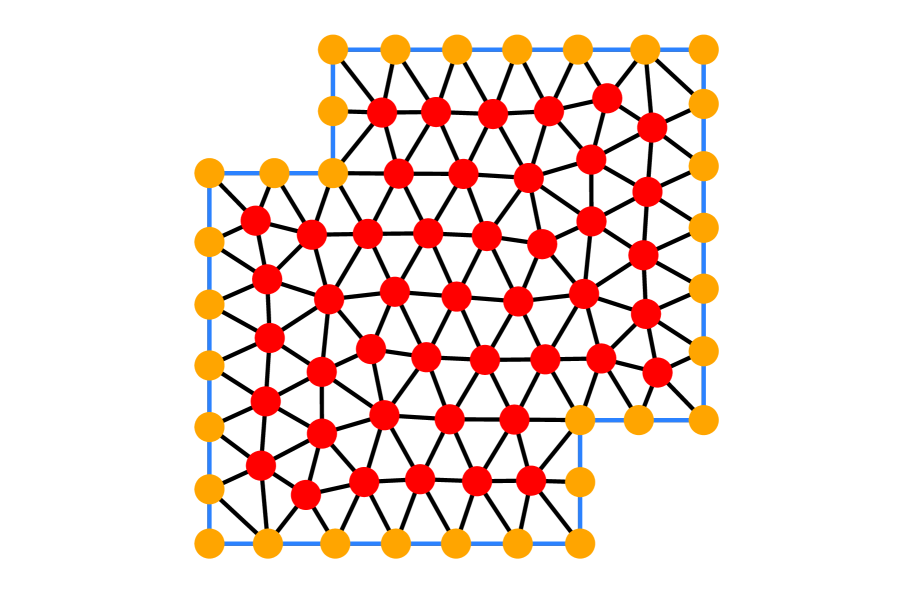
(b) Step 0: initial state

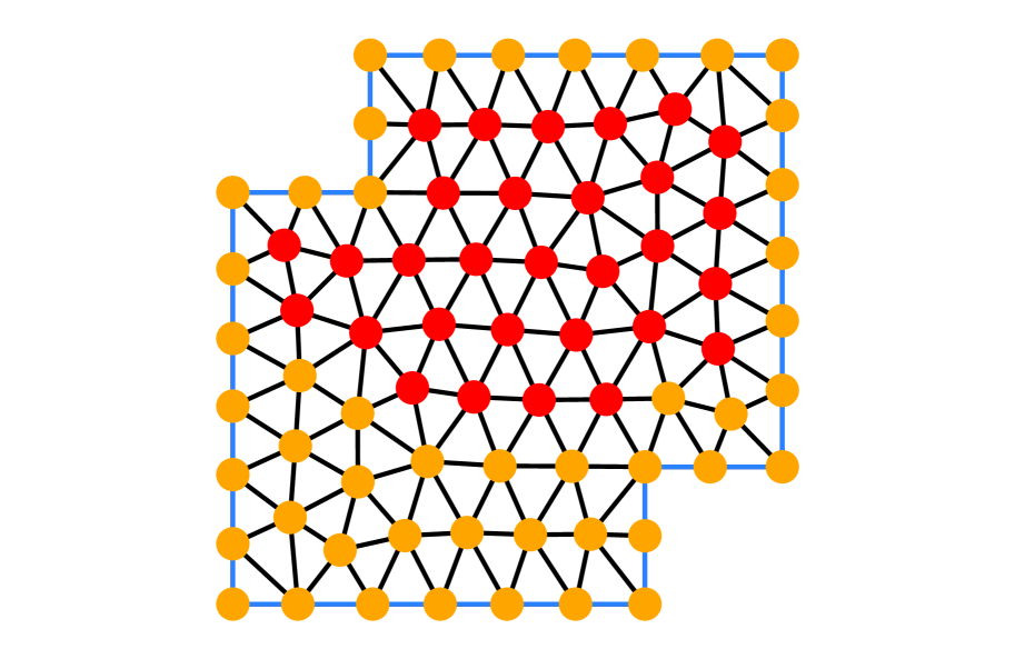
(c) Step 15

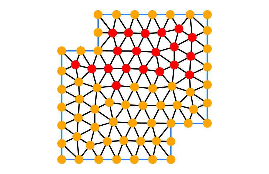
(d) Step 25

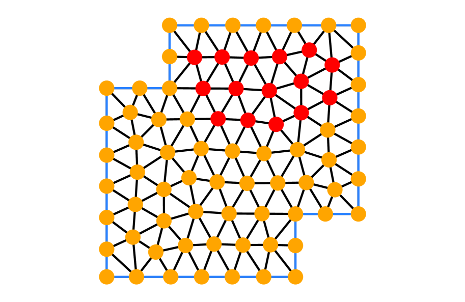
(e) Step 30

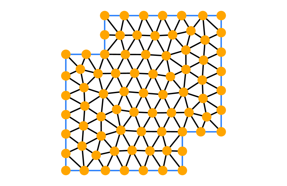
(f) Step 45: final state

Figure 10: Example of a non-convex geometry and the evolution of Algorithm MOTZ (with result MOTZ_result = certified).

Figure 11 shows the mesh of a geometry with one hole. As before, the boundary with Robin boundary conditions is illustrated in blue (note, that the hole has Robin boundary conditions as well) and we initialize the algorithm with $\mathcal{N}_{\operatorname*{test}}:=\mathcal{N}\cap\Gamma$. Also in this example, MOTZ returns MOTZ_result = certified which means that problem (15) is well posed. In the following we refer to the nodes in $\mathcal{N}_{\operatorname*{dof}}$ (red nodes) that are connected by an edge to the boundary nodes of the inner circle as ‘layer 1’ nodes, ‘layer 0’ being the boundary nodes on the circle. Interestingly, none of the ‘layer 1’ nodes can be marked orange initially, since each boundary node on the circle is connected to at least two ‘layer 1’ nodes and therefore has a transmission degree larger than one. Thus, MOTZ has to start from the outer boundary and successively moves towards the interior boundary points. Only in step 62 of the algorithm (see Figure 11(c)) one entry point into ‘layer 1’ can be found. Note that none of the other nodes in ‘layer 1’ could have been marked orange at this point, since all of the orange ‘layer 2’ nodes, except the one, have transmission degree 2 (are connected to two red nodes).

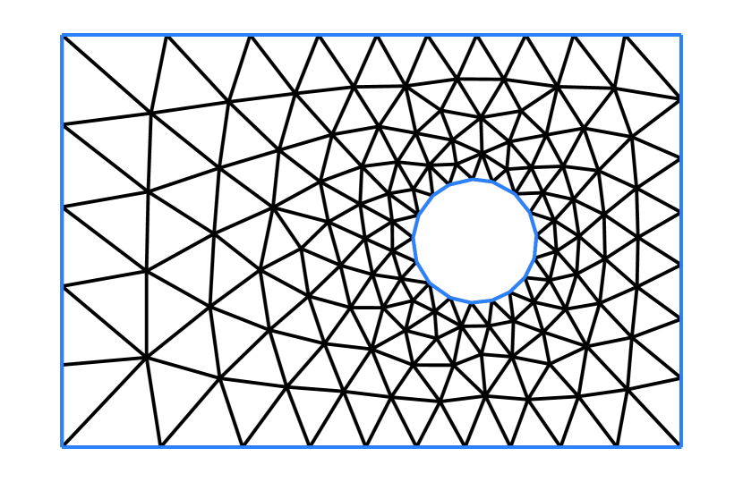
(a) Mesh with boundary

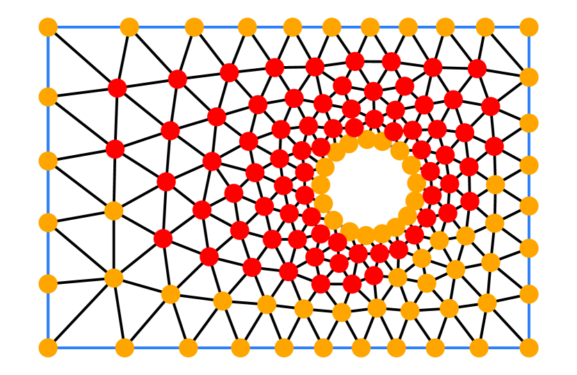
(b) Step 20

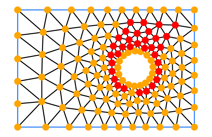
(c) Step 62

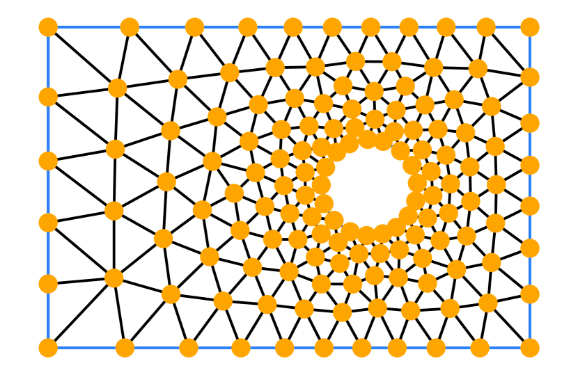
(d) Step 95: final state

Figure 11: Example of a non-convex geometry with one hole and the evolution of Algorithm MOTZ (with result MOTZ_result = certified).

This suggests how a finite element mesh would need to look like in order for MOTZ to give the result MOTZ_result = critical. If the mesh in Figure 11(a) was such that each ‘layer 1’ node is connected to exactly two nodes in ‘layer 0’ and ‘layer 2’, the algorithm would not find any entry point into ‘layer 1’ and would return MOTZ_result = critical. However, in practice we could not produce such a mesh with standard mesh generation tools due to the non-optimal quality of the desired mesh.

We applied the Algorithm MOTZ to various geometries and mesh configurations (sharp corners, complex geometries, strong local refinements). None of the tested meshes that were produced by a standard mesh generation algorithm (such as [SH21, Sch22]), actually led to the output MOTZ_result = critical of the Algorithm MOTZ.

4.2 A mesh modification algorithm and numerical experiments

Even though the algorithm seems to return the output MOTZ_result = certified for most shape regular meshes, one can construct examples where it returns a critical result. In this section, we are in particular interested in the case where this is due to the output MOTZ_trans = false, i.e. where no more edges which satisfy condition (a) of Lemma 4.3 could be found. In these cases we need to modify the finite element mesh so that the corresponding Galerkin discretization has a unique solution. We propose the following three simple mesh modification strategies, that can lead to a passing of the checking algorithm:

• Re-building of the whole mesh with slightly modified mesh parameters.

• Local refinement of the mesh across the interface of $\mathcal{N}_{\operatorname*{dof}}$ and $\mathcal{N}\backslash\mathcal{N}_{\operatorname*{dof}}$, where $\mathcal{N}_{\operatorname*{dof}}$ is the result of MOTZ.

• Application of Algorithm 3 (MOTZ_flip), which flips certain edges at the interface of $\mathcal{N}_{\operatorname*{dof}}$ and $\mathcal{N}\backslash\mathcal{N}_{\operatorname*{dof}}$.

If MOTZ returns MOTZ_trans = false (together with the non-empty set $\mathcal{N}_{\operatorname*{dof}}$), the algorithm was not able to find any more nodes that satisfy condition (a) of Lemma 4.3. The idea behind all three strategies above is to alter existing or create new entry points for the algorithm into the remaining set $\mathcal{N}_{\operatorname*{dof}}$. Re-building of the whole mesh with slightly different parameters or a different meshing algorithm is a simple way of altering triangles and edges which in turn might break up the constellations that lead to the output MOTZ_result = critical. If this is not possible or not successful, a more targeted local refinement around a node on the boundary of $\mathcal{N}_{\operatorname*{dof}}$ might lead to new entry points and to a passing of the checking algorithm.
A highly targeted approach to create new entry points with minimal modifications to the original mesh is described in Algorithm 3. The idea is to detect those nodes on the boundary of $\mathcal{N}_{\operatorname*{dof}}$ that have exactly two connected nodes in $\mathcal{N}_{\operatorname*{test}}$, which in turn have exactly one common node in $\mathcal{N}_{\operatorname*{test}}$ (see Figure 12). Flipping the interior edge in this scenario, i.e., replacing $[z_{1},z_{2}]$ with $[z,\tilde{z}]$, will then increase the transmission degree of $\tilde{z}$ by one. Since this will typically mean that $\deg\left(\tilde{z},\mathcal{N}_{\operatorname*{test}}\right)=1$, this mesh modification will create a new entry point for MOTZ into $\mathcal{N}_{\operatorname*{dof}}$. Often, the constellation described in Figure 12 can be found multiple times in a mesh. In Algorithm 3 we propose to compute a mesh quality score for each potential edge flip (e.g. based on minimal angles of the resulting triangles). MOTZ is then rerun for the modified mesh with the highest quality score.

Figure 12: Replacing $[z_{1},z_{2}]$ with $[z,\tilde{z}]$ increases $\deg\left(\tilde{z},\mathcal{N}_{\operatorname{test}}\right)$ by 1 ( $\in\mathcal{N}_{\operatorname{test}}$, $\in\mathcal{N}_{\operatorname{dof}}$).

Algorithm 3 makes use of the following definitions:

1. The neighbouring nodes of a node $z\in\mathcal{N}$ are denoted by

   $$\mathcal{N}_{\operatorname{neighbours}}(z)=\{z^{\prime}\in\mathcal{N}\backslash\{z\}\mid[z,z^{\prime}]\in\mathcal{E}_{\Omega}\}.$$

2. The set of edges $\mathcal{E}_{\Omega}$, where edge $[z_{1},z_{2}]$ has been replaced by edge $[\tilde{z}_{1},\tilde{z}_{2}]$ is denoted by

   $$\mathcal{E}_{\Omega,[z_{1},z_{2}]\rightarrow[\tilde{z}_{1},\tilde{z}_{2}]}:=\mathcal{E}_{\Omega}\backslash\{[z_{1},z_{2}]\}\cup\{[\tilde{z}_{1},\tilde{z}_{2}]\}.$$

Algorithm 3 MOTZ_flip

Input: MOTZ_result, $\mathcal{N}_{\operatorname{dof}}$, $\mathcal{N}_{\operatorname{test}}$, $\mathcal{N}$, $\mathcal{E}_{\Omega}$
    Output: updated MOTZ_result, $\mathcal{N}_{\operatorname{dof}}$, $\mathcal{N}_{\operatorname{test}}$, $\mathcal{N}$, $\mathcal{E}_{\Omega}$

1:  while MOTZ_result = critical do

2:     Set $\mathcal{P}=\{\}$, which will hold possible modified meshes, together with a quality score for each mesh.

3:     for all $z\in\partial\mathcal{N}_{\operatorname{dof}}$ do

4:        Let $z$ have exactly two neighbours in $\mathcal{N}_{\operatorname{test}}$, denoted by $z_{1},z_{2}\in\mathcal{N}_{\operatorname{neighbours}}(z)\cap\mathcal{N}_{\operatorname{test}}$

5:        if $\mathcal{N}_{\operatorname{neighbours}}(z_{1})\cap\mathcal{N}_{\operatorname{neighbours}}(z_{2})\cap\mathcal{N}_{\operatorname{test}}=\{\tilde{z}\}$ then

6:           Compute a quality score $q$ for the mesh associated with $\mathcal{E}_{\Omega,[z_{1},z_{2}]\rightarrow[z,\tilde{z}]}$

7:           Set $\mathcal{P}=\mathcal{P}\cup\{({\mathcal{E}_{\Omega,[z_{1},z_{2}]\rightarrow[z,\tilde{z}]},q})\}$

8:        end if

9:     end for

10:     if $\mathcal{P}=\{\}$ then

11:        STOP

12:     else

13:        Let $\mathcal{E}^{\max}_{\Omega,[z_{1},z_{2}]\rightarrow[z,\tilde{z}]}$ be the set of edges in $\mathcal{P}$ with the highest quality score.

14:        (MOTZ_result, $\mathcal{N}_{\operatorname{dof}}$, $\mathcal{N}_{\operatorname{test}}$, $\mathcal{N}$, $\mathcal{E}_{\Omega}$) = MOTZ($\mathcal{N}_{\operatorname{test}}$, $\mathcal{N}$, $\mathcal{E}^{\max}_{\Omega,[z_{1},z_{2}]\rightarrow[z,\tilde{z}]}$)

15:     end if

16:  end while

We emphasize that the strategies described above are heuristic, e.g., only the case of two neighbours is considered in Algorithm 3: line 5. However, we expect that they are successful in the vast majority of cases where MOTZ returns MOTZ_trans = false.

Figure 13(a) shows an example of a mesh, where the checking algorithm returns MOTZ_result = critical, together with a non-empty set $\mathcal{N}_{\operatorname*{dof}}$ consisting of four points (see Figure 13(b) ). We apply Algorithm 3 MOTZ_flip, which in this case will detect four edges that can potentially be flipped. As a simple quality score we measure the minimal angle for each triangle in the mesh. Due to the symmetry of the mesh, the quality score for each potential modification suggested by MOTZ_flip coincides. Therefore, there is no preference concerning the choice of the edge that will be flipped in this case. Figure 13(c) shows the modified mesh. Indeed, this modification is sufficient in order for MOTZ to return MOTZ_result = certified.

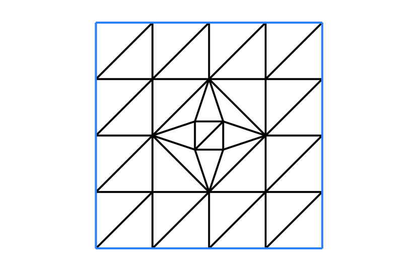
(a) Original mesh

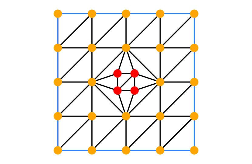
(b) MOTZ returns MOTZ_result = critical.

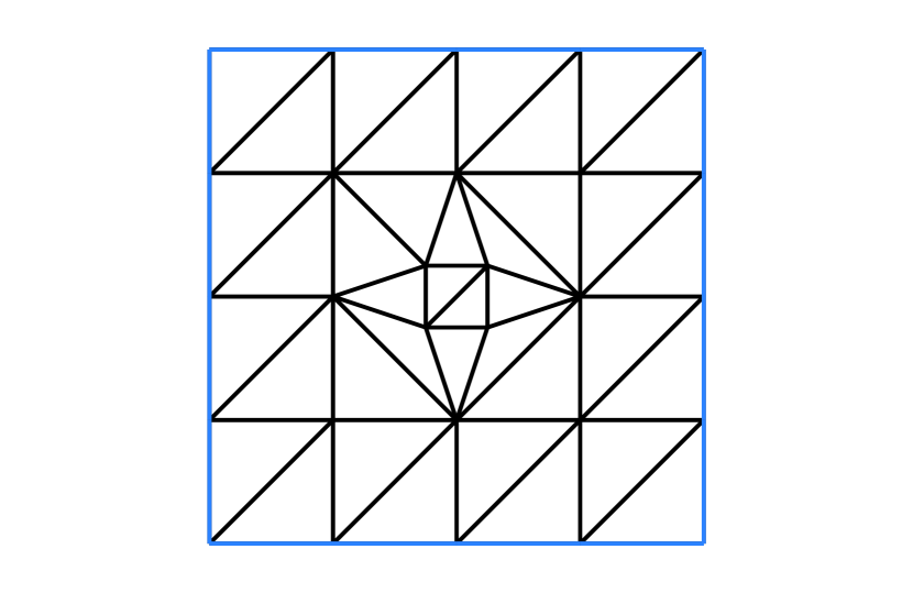
(c) Modified mesh

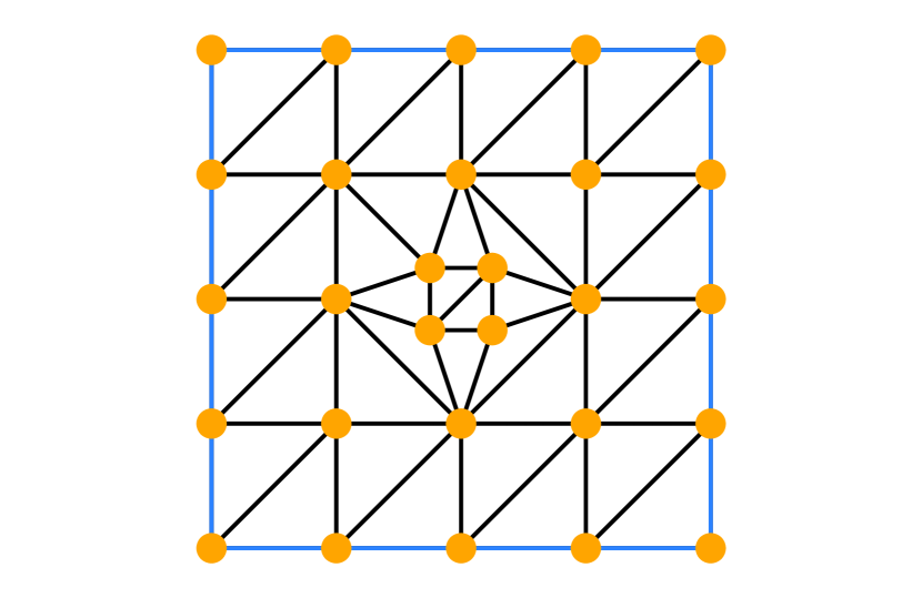
(d) MOTZ returns MOTZ_result = certified.

Figure 13: (a) Example of a mesh for which MOTZ returns MOTZ_result = critical. (c) Modified mesh as a result of Algorithm 3 which leads to a passing checking algorithm.

Below we consider the impact of mesh modification via Algorithm 3 MOTZ_flip by numerically calculating the reciprocal of the discrete inf-sup constant $\beta_{k}$ given by

$$\beta_{k}:=\inf_{u_{h}\in S_{\mathcal{T}}^{1}}\,\sup_{v_{h}\in S_{\mathcal{T}}^{1}}\,\frac{a_{k}(u_{h},v_{h})}{\|u_{h}\|_{1,k,\Omega}\|v_{h}\|_{1,k,\Omega}},$$

for a modification of the mesh considered in Section 3.2 for $\alpha=\tfrac{1}{2}$. The $k$-weighted natural norm $\|\cdot\|_{1,k,\Omega}$ on $H^{1}(\Omega)$ is given by $\|u\|_{1,k,\Omega}:=\left(\|\nabla u\|_{L^{2}(\Omega)}^{2}+k^{2}\|u\|_{L^{2}(\Omega)}^{2}\right)^{1/2}$ for $u\in H^{1}(\Omega)$. The discrete inf-sup constant $\beta_{k}$ can be numerically calculated via a generalized eigenvalue problem.

For the mesh considered in Section 3.2 with $\alpha=\tfrac{1}{2}$, we find that $k=6$ results in a singular system matrix, see equation (7). We inscribe the mesh considered in Section 3.2 into another quadrilateral, see Figure 14, in order to apply Algorithm 3 MOTZ_flip. For the left mesh in Figure 14 MOTZ returns MOTZ_result = critical. The numerical results are visualized in Figure 15. We observe that for $k=6$ the original mesh results in a singular system matrix, while the modified mesh from MOTZ_flip results in a regular one.

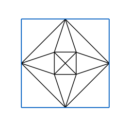
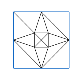
Figure 14: For the mesh on the left, MOTZ returns MOTZ_result = critical. The mesh on the right is the result of MOTZ_flip.

Figure 15: Plot of $k$ against $\tfrac{1}{\beta_{k}}$ for the meshes as in Figure 14.

The algorithms MOTZ and MOTZ_flip have been implemented in Python. The code is available via https://github.com/alexander-veit/MOTZ.

References

- [BBHP19] Alex Bespalov, Timo Betcke, Alexander Haberl, and Dirk Praetorius. Adaptive BEM with optimal convergence rates for the Helmholtz equation. Comput. Methods Appl. Mech. Engrg., 346:260–287, 2019.
- [BS08] Susanne C. Brenner and L. Ridgway Scott. The mathematical theory of finite element methods, volume 15 of Texts in Applied Mathematics. Springer, New York, third edition, 2008.
- [BWZ16] Erik Burman, Haijun Wu, and Lingxue Zhu. Linear continuous interior penalty finite element method for Helmholtz equation with high wave number: one-dimensional analysis. Numer. Methods Partial Differential Equations, 32(5):1378–1410, 2016.
- [CFEV21] Théophile Chaumont-Frelet, Alexandre Ern, and Martin Vohralík. On the derivation of guaranteed and p-robust a posteriori error estimates for the Helmholtz equation. Numerische Mathematik, 2021.
- [Cia78] Philippe G. Ciarlet. The finite element method for elliptic problems. Studies in Mathematics and its Applications, Vol. 4. North-Holland Publishing Co., Amsterdam-New York-Oxford, 1978.
- [CQ17] Huangxin Chen and Weifeng Qiu. A first order system least squares method for the Helmholtz equation. J. Comput. Appl. Math., 309:145–162, 2017.
- [DS13] Willy Dörfler and Stefan A. Sauter. A posteriori error estimation for highly indefinite Helmholtz problems. Comput. Methods Appl. Math., 13(3):333–347, 2013.
- [FW11] Xiaobing Feng and Haijun Wu. -discontinuous Galerkin methods for the Helmholtz equation with large wave number. Math. Comp., 80(276):1997–2024, 2011.
- [IB95] F. Ihlenburg and I. Babuška. Finite Element Solution to the Helmholtz Equation with High Wave Number. Part I: The -version of the FEM. Comp. Math. Appl., 39(9):9–37, 1995.
- [IB97] F. Ihlenburg and I. Babuška. Finite Element Solution to the Helmholtz Equation with High Wave Number. Part II: The - version of the FEM. SIAM J. Num. Anal., 34(1):315–358, 1997.
- [IB01] S. Irimie and Ph. Bouillard. A residual a posteriori error estimator for the finite element solution of the Helmholtz equation. Comput. Methods Appl. Mech. Engrg., 190(31):4027–4042, 2001.
- [Lei86] R. Leis. Initial Boundary Value Problems in Mathematical Physics. Teubner, Wiley Sons, Stuttgart, Chichester, 1986.
- [LZ21] Linjun Li and Lingfu Zhang. Anderson-Bernoulli localization on the 3d lattice and discrete unique continuation principle. ArXiv: 1906.04350, 2021.
- [Mel95] J. M. Melenk. On Generalized Finite Element Methods. PhD thesis, University of Maryland at College Park, 1995.
- [MPS13] J. M. Melenk, A. Parsania, and S. A. Sauter. General DG-methods for highly indefinite Helmholtz problems. J. Sci. Comput., 57(3):536–581, 2013.
- [MS10] J. M. Melenk and S. A. Sauter. Convergence Analysis for Finite Element Discretizations of the Helmholtz equation with Dirichlet-to-Neumann boundary condition. Math. Comp, 79:1871–1914, 2010.
- [MS11] J. M. Melenk and S. A. Sauter. Wave-Number Explicit Convergence Analysis for Galerkin Discretizations of the Helmholtz Equation. SIAM J. Numer. Anal., 49(3):1210–1243, 2011.
- [Sau89] S. Sauter. Ein Mehrgitterverfahren zur Berechnung der Eigenschwingungen von abgeschlossenen Wasserbecken. Diplomarbeit, Universität Heidelberg, 1989.
- [Sch74] A.H. Schatz. An observation concerning Ritz-Galerkin methods with indefinite bilinear forms. Math. Comp., 28:959–962, 1974.
- [Sch22] Nico Schlömer. optimesh: Optimization for simplex meshes. optimesh: Optimization for simplex meshes (v0.8.6). Zenodo. https://doi.org/10.5281/zenodo.5884995, January 2022.
- [SEP98] Christoph Stamm, Stephan Eidenbenz, and Renato Pajarola. A modified longest side bisection triangulation. Electronic Proceedings of the 10th Canadian Conference on Computational Geometry, 1998.
- [SF73] G. Strang and G.J. Fix. An Analysis of the Finite Element Method. Prentice-Hall, Englewood Cliffs, 1973.
- [SH21] Nico Schlömer and J. Hariharan. dmsh: Simple mesh generator inspired by distmesh. dmsh: Simple mesh generator inspired by distmesh (v0.2.14). Zenodo. https://doi.org/10.5281/zenodo.4728040, April 2021.
- [SZ15] S. A. Sauter and J. Zech. A posteriori error estimation of -dG finite element methods for highly indefinite Helmholtz problems. SIAM J. Numer. Anal., 53(5):2414–2440, 2015.
- [Wu14] Haijun Wu. Pre-asymptotic error analysis of CIP-FEM and FEM for the Helmholtz equation with high wave number. Part I: linear version. IMA J. Numer. Anal., 34(3):1266–1288, 2014.
- [XZ99] Jinchao Xu and Ludmil Zikatanov. A monotone finite element scheme for convection-diffusion equations. Math. Comp., 68(228):1429–1446, 1999.