Polarimetric properties of Event Horizon Telescope targets from ALMA

Abstract

We present the results from a full polarization study carried out with the Atacama Large Millimeter/submillimeter Array (ALMA) during the first Very Long Baseline Interferometry (VLBI) campaign, which was conducted in Apr 2017 in the $\lambda$3 mm and $\lambda$1.3 mm bands, in concert with the Global mm-VLBI Array (GMVA) and the Event Horizon Telescope (EHT), respectively. We determine the polarization and Faraday properties of all VLBI targets, including Sgr A*, M87, and a dozen radio-loud AGN, in the two bands at several epochs in a time window of ten days. We detect high linear polarization fractions (2–15%) and large rotation measures (RM $>10^{3.3}-10^{5.5}$ rad m^-2), confirming the trends of previous AGN studies at mm wavelengths. We find that blazars are more strongly polarized than other AGN in the sample, while exhibiting (on average) an order-of-magnitude lower RM values, consistent with the AGN viewing angle unification scheme. For Sgr A* we report a mean RM of $(-4.2\pm 0.3)\times 10^{5}$ rad m^-2 at 1.3 mm, consistent with measurements over the past decade, and, for the first time, a RM of $(-2.1\pm 0.1)\times 10^{5}$ rad m^-2 at 3 mm, suggesting that about half of the Faraday rotation at 1.3 mm may occur between the 3 mm photosphere and the 1.3 mm source. We also report the first unambiguous measurement of RM toward the M87 nucleus at mm wavelengths, which undergoes significant changes in magnitude and sign reversals on a one year time-scale, spanning the range from –1.2 to 0.3 $\times\,10^{5}$ rad m^-2 at 3 mm and –4.1 to 1.5 $\times\,10^{5}$ rad m^-2 at 1.3 mm. Given this time variability, we argue that, unlike the case of Sgr A*, the RM in M87 does not provide an accurate estimate of the mass accretion rate onto the black hole. We put forward a two-component model, comprised of a variable compact region and a static extended region, that can simultaneously explain the polarimetric properties observed by both the EHT (on horizon scales) and ALMA (which observes the combined emission from both components). These measurements provide critical constraints for the calibration, analysis, and interpretation of simultaneously obtained VLBI data with the EHT and GMVA.

1 Introduction

Active galactic nuclei (AGN) are known to host supermassive black holes (SMBHs), which accrete gas through a disk and drive powerful relativistic jets that are observed on scales of parsecs to megaparsecs (Blandford et al. 2019). Magnetic fields are believed to play a major role in the formation of such relativistic jets, by either extracting energy from a spinning SMBH via the Blandford–Znajek mechanism (Blandford & Znajek 1977) or by tapping into the rotational energy of a magnetized accretion flow via the Blandford–Payne mechanism (Blandford & Payne 1982).

Polarization observations are a powerful tool to probe magnetic fields and to understand their role in black-hole mass-accretion and launching and acceleration of relativistic AGN jets. In fact, the radio emission from AGN and their associated jets is thought to be produced by synchrotron processes, and thus they display high intrinsic linear polarization (LP; e.g., Pacholczyk 1970; Trippe et al. 2010; Agudo et al. 2018). LP fractions and polarization vector orientations can provide details on the magnetic field strength and topology. Besides LP, circular polarization (CP) may also be present as a consequence of Faraday conversion of the linearly-polarized synchrotron emission (Beckert & Falcke 2002), and can also help constraining the magnetic field configuration (e.g., Muñoz et al. 2012).

As the linearly polarized radiation travels through magnetized plasma, it experiences Faraday rotation of the LP vectors. The externally magnetized plasma is also known as the “Faraday screen” and the amount of Faraday rotation is known as the “rotation measure” (RM). If the background source of polarized emission is entirely behind (and not intermixed with) the Faraday screen, the RM can be written as an integral of the product of the electron number density ($n_{e}$) and the magnetic field component along the line-of-sight ($B_{||}$) via:

$$\mathrm{RM}=8.1\times 10^{5}\int n_{e}[\mathrm{cm^{-3}}]~{}\mathbf{B}[\mathrm{G}]\cdot\mathbf{\mathrm{d}l}[\mathrm{pc}]~{}~{}\mathrm{rad\,m}^{-2}\,.$$ (1)

Thus, by measuring the RM one can also constrain the electron density, $n_{e}$, and the magnetic field, $B_{||}$, in the plasma surrounding SMBHs. Under the assumption that the polarized emission is produced close to the SMBH and then Faraday-rotated in the surrounding accretion flow, the RM has been used in some cases to infer the accretion rate onto SMBHs (e.g, Marrone et al. 2006, 2007; Plambeck et al. 2014; Kuo et al. 2014; Bower et al. 2018). Alternatively, the polarized emission may be Faraday-rotated along the jet boundary layers (e.g., Zavala & Taylor 2004; Martí-Vidal et al. 2015). Therefore, Faraday rotation measurements can provide crucial constraints on magnetized accretion models and jet formation models.

RM studies are typically conducted at cm wavelengths using the Very Large Array (VLA) or the Very Long Baseline Array (VLBA; e.g., Zavala & Taylor 2004). However, cm wavelengths are strongly affected by synchrotron self-absorption (SSA) close to the central engines and can therefore only probe magnetized plasma in the optically thin regions at relatively larger distances (parsec scales) from the SMBH (Gabuzda et al. 2017; Kravchenko et al. 2017). On the other hand, emission at mm wavelengths is optically thin from the innermost regions of the jet base (and accretion disc), enabling us to study the plasma and magnetic fields much closer to the SMBH. In addition, LP can be more easily detected at mm wavelengths because the mm emission region is smaller (e.g., Lobanov 1998), and so depolarization induced by RM variations across the source (e.g., owing to a tangled magnetic field) is less significant. Finally, since Faraday rotation is smaller at shorter wavelengths (with a typical $\lambda^{2}$ dependence), mm-wavelength measurements more clearly reflect the intrinsic LP properties, and therefore the magnetic field of the system.

Unfortunately, polarimetric measurements at mm wavelengths have so far been limited by sensitivity and instrumental systematics. The first interferometric measurements of RM at (sub)mm wavelengths were conducted towards Sgr A* with the Berkeley-Illinois-Maryland Association (BIMA) array (Bower et al. 2003, 2005) and the Submillimeter Array (SMA Marrone et al. 2006, 2007), which yielded a RM $\sim-5\times 10^{5}$ rad m^-2. SMA measurements towards M87 provided an upper limit $\left|{\rm RM}\right|<7.5\times 10^{5}$ rad m^-2 (Kuo et al. 2014). Other AGN with RM detections with mm interferometers include 3C 84 with RM $=8\times 10^{5}$ rad m^-2 (Plambeck et al. 2014; see also Nagai et al. 2017 for a similarly high RM measured with the VLBA at 43 GHz), PKS 1830-211 (at a redshift $z=2.5$) with RM $\sim 10^{7}$ rad m^-2  (Martí-Vidal et al. 2015), and 3C 273 with RM $=5\times 10^{5}$ rad m^-2 (Hovatta et al. 2019). Additional examples of AGN RM studies with mm single-dish telescopes can be found in Trippe et al. (2012) and Agudo et al. (2018).

In order to progress in this field, polarization interferometric studies at mm wavelengths should be extended to a larger sample of AGN and it will be important to investigate both time and frequency dependence effects, by carrying out observations at multiple frequency bands and epochs. Ultimately, observational studies should be conducted at the highest possible angular resolutions in order to resolve the innermost regions of the accretion flow and/or the base of relativistic jets.

The advent of the Atacama Large Millimeter/ submillimeter Array (ALMA) as a phased array (hereafter phased-ALMA; Matthews et al. 2018; Goddi et al. 2019a) as a new element to Very Long Baseline Interferometry (VLBI) at millimeter (mm) wavelengths (hereafter mm-VLBI) has been a game charger in terms of sensitivity and polarimetric studies. In this paper, we present a complete polarimetric analysis of ALMA observations carried out during the first VLBI campaign.

1.1 mm-VLBI with ALMA

The first science observations with phased-ALMA were conducted in April 2017 (Goddi et al. 2019a), in concert with two different VLBI networks: the Global mm-VLBI Array (GMVA) operating at 3 mm wavelength (e.g., Marti-Vidal et al. 2012) and the Event Horizon Telescope (EHT) operating at 1.3 mm wavelength (Event Horizon Telescope Collaboration et al. 2019a). These observations had two “key science” targets, the SMBH candidate at the Galactic center, Sgr A*, and the nucleus of the giant elliptical galaxy M87 in the Virgo cluster, M87*, both enabling studies at horizon-scale resolution (Doeleman et al. 2008, 2012; Goddi et al. 2017; Event Horizon Telescope Collaboration et al. 2019b). In addition to those targets, VLBI observations with phased-ALMA also targeted a sample of a dozen radio-loud AGN, including the closest and most luminous quasar 3C 273, the bright $\gamma$-ray-emitting blazar 3C 279, the closest radio-loud galaxy Centaurus A (Cen A), and the best supermassive binary black hole candidate OJ287.

In 2019, the first EHT observations with phased-ALMA yielded groundbreaking results, most notably the first ever event-horizon-scale image of the M87* SMBH (Event Horizon Telescope Collaboration et al. 2019b, a, c, d, e, f). Beyond this breakthrough, EHT observations have now imaged polarized emission in the ring surrounding M87*, resolving for the first time the magnetic field structures within a few Schwarzschild radii ($R_{Sch}$) of a SMBH (Event Horizon Telescope Collaboration et al. 2021a). In addition, these new polarization images enable us to place tight constraints on physical models of the magnetized accretion flow around the M87* SMBH and, in general, on relativistic jet launching theories (Event Horizon Telescope Collaboration et al. 2021b).

Both the VLBI imaging and the theoretical modelling use constraints from ALMA observations (Event Horizon Telescope Collaboration et al. 2021a, b). In fact, besides providing a huge boost in sensitivity and uv-coverage (Event Horizon Telescope Collaboration et al. 2019c; Goddi et al. 2019b), the inclusion of ALMA in a VLBI array provides another important advantage: standard interferometric visibilities among the ALMA antennas are computed by the ALMA correlator and simultaneously stored in the ALMA archive together with the VLBI recording of the phased signal (Matthews et al. 2018; Goddi et al. 2019a). Furthermore, VLBI observations are always performed in full-polarization mode in order to supply the inputs to the polarization conversion process (from linear to circular) at the VLBI correlators, which is carried out using the PolConvert software (Martí-Vidal et al. 2016) after the ”Level 2 Quality Assurance” (QA2) process (Goddi et al. 2019a). Therefore, VLBI observations with ALMA yield a full-polarization interferometric dataset, which provides both source-integrated information for refinement and validation of VLBI data calibration (Event Horizon Telescope Collaboration et al. 2021a) as well as observational constraints to theoretical models (Event Horizon Telescope Collaboration et al. 2021b). Besides these applications, this dataset carries valuable scientific value on its own and can be used to derive mm emission, polarization, and Faraday properties of a selected sample of AGN on arcsecond scales.

1.2 This paper

In this paper, we present a full polarization study carried out with ALMA in the $\lambda$3 mm and $\lambda$1 mm bands towards Sgr A*, M87, and a dozen radio-loud AGN, with particular emphasis on their polarization and Faraday properties. The current paper is structured as follows.

Section 2 summarizes the 2017 VLBI observations (§2.1), the procedures followed for the data calibration (§2.2), the details of the full-polarization image deconvolution (§2.3), and additional observations on M87 (§2.4).

Section 3 describes the procedures of data analysis. After presenting some representative total-intensity images of Sgr A* and M87 (§3.1), two independent algorithms to estimate the Stokes parameters of the compact cores are described (§3.2). The Stokes parameters for each source and spectral window are then converted into fractional LP and EVPA (§3.3.1), and used to estimate Faraday rotation (§3.3.2) and (de)polarization effects (§3.3.3). Finally, the CP analysis is summarised in §3.3.4.

Section 4 reports the polarimetric and Faraday properties of all the GMVA and EHT target sources, with dedicated subsections on AGN, M87, and Sgr A*.

In Section 5, the polarization properties presented in the previous sections are used to explore potential physical origins of the polarized emission and location of Faraday screens in the context of SMBH accretion and jet formation models. §5.1.1 presents a comparison between the $\lambda$3 mm and $\lambda$1.3 mm bands, including a discussion on the effects of synchrotron opacity and Faraday rotation; §5.1.2 presents a comparison between the case of blazars and other AGN; §5.1.3 discusses about depolarization in radio galaxies and its possible connection to instrumental effects. §5.2 is devoted to the special case of M87, including a discussion about the origin of the Faraday screen (internal vs. external; §5.2.1) as well as a simple two-component Faraday model (§5.2.2). Finally, §5.3 is dedicated to the special case of Sgr A*.

Conclusions are drawn in Section 6.

The paper is supplemented with a number of appendices including: the list of ALMA projects observed during the VLBI campaign in April 2017 (Appendix A), a full suite of polarimetric images (B) for all the observed targets, comparisons between multiple flux-extraction methods (C) and between the polarimetry results obtained during the VLBI campaign and the monitoring programme with the Atacama Compact Array (D), tables with polarimetric quantities per ALMA spectral-window (E), Faraday RM plots (F), quality assessment of the circular polarization estimates (G), and mm spectral indices of all the observed targets (H). Finally, a two-component polarization model for M87, which combines constraints from ALMA and EHT observations, is presented in Appendix I.

2 Observations, data processing, and imaging

2.1 2017 VLBI observations with ALMA

The observations with phased-ALMA were conducted as part of Cycle 4 during the 2017 VLBI campaign in ALMA Band 3 (April 1-3) and Band 6 (April 5-11), respectively. The ALMA data were acquired simultaneously with the VLBI observations (in this sense they are a “byproduct” of the VLBI operations). The ALMA array was in the compact configurations C40-1 (with 0.15 km longest baseline) and, after Apr 6, C40-3 (with 0.46 km longest baseline). Only antennas within a radius of 180 m (from the array center) were used for phasing on all days. About 37 antennas were normally phased together, which is equivalent to a telescope of 73 m diameter. In both Band 3 and 6, the spectral setup includes four spectral windows (SPWs) of 1875 MHz, two in the lower and two in the upper sideband, correlated with 240 channels per SPW (corresponding to a spectral resolution of 7.8125 MHz). In Band 3 the four SPWs are centered at 86.268, 88.268, 98.328, and 100.268 GHz while in Band 6 they are centered at 213.100, 215.100, 227.100, and 229.100 GHz.

Three projects were observed in Band 3 with the GMVA (science targets: OJ 287, Sgr A*, 3C 273) and six projects were observed in Band 6 with the EHT (science targets: OJ 287, M87, 3C 279, Sgr A*, NGC 1052, Cen A). The projects were arranged and calibrated in “tracks” (where one track consists of the observations taken during the same day/session). In Appendix A we provide a list of the observed projects and targets on each day, with the underlying identifications of (calibration and science target) sources within each project (see Tables 4 and 5 in Appendix A). More details of the observation structure and calibration sources can be found in Goddi et al. (2019a).

2.2 Data calibration and processing

During phased-array operations, the data path from the antennas to the ALMA correlator is different with respect to standard interferometric operations (Matthews et al. 2018; Goddi et al. 2019a). This makes the calibration of VLBI observations within the Common Astronomy Software Applications (casa) package intrinsically different and some essential modification in the procedures is required with respect to ALMA standard observations. The special steps added to the standard ALMA polarization calibration procedures (e.g., Nagai et al. 2016) are described in detail in Goddi et al. (2019a). The latter focus mostly on the LP calibration and the polarization conversion at the VLBI correlators (Martí-Vidal et al. 2016). In this paper we extend the data analysis also to the CP.

Only sources observed in VLBI mode were calibrated in polarization (see Section 5 in Goddi et al. 2019a). Therefore the sources exclusively observed for ordinary ALMA calibration during the VLBI schedule gaps (i.e., Flux and Gain calibrators) are excluded from this analysis (compare the source list in Tables 4 and 5 in Appendix A with Tables 4 and 6 in Goddi et al. 2019a). Two additional sources observed on Apr 7, 3C 84 and J0006-0623, are also excluded from the following analysis. These sources are in fact flagged in a final flagging step (run on the fully calibrated $uv$-data before imaging and data analysis), which removes visibility data points having amplitudes outside a certain range (set by three times the RMS from the median of the data) and a source elevation below 25^∘. Finally, the two weakest targets observed at 1.3 mm, NCG 1052 and J0132-1654, were found to fall below the flux threshold (correlated flux density of $>$0.5 Jy on intra-ALMA baselines) required to enable on-source phasing of the array as commissioned (Matthews et al. 2018). Despite these two sources are detected with high signal-to-noise ratio (SNR) in total intensity (SNR$>1000$) and polarized flux (SNR$>50$ for J0132-1654), we recommend extra care in interpreting these source measurements owing to lower data quality.

2.3 Full-stokes imaging

All targets observed in Band 3 and Band 6 are imaged using the casa task tclean in all Stokes parameters: $I$, $Q$, $U$, $V$. A Briggs weighting scheme (Briggs 1995) is adopted with a robust parameter of 0.5, and a cleaning gain of 0.1. A first quick cleaning (100 iterations over all four Stokes parameters) is done in the inner 10″ and 4″  in bands 3 and 6, respectively. Providing there is still significant emission ($>7\sigma$) in the residual maps (e.g., in M87 and Sgr A*), an automatic script changes the cleaning mask accordingly, and a second, deeper cleaning is done down to 2$\sigma$ (these two clean steps are run with parameter interactive=False). A final interactive clean step (with interactive=True) is run to adjust the mask to include real emission which was missed by the automatic masking and to clean deeper sources with complex structure and high-signal residuals (this step was essential for proper cleaning of Sgr A*). No self-calibration was attempted during the imaging stage (the default calibration scheme for ALMA-VLBI data already relies on self-calibration; see Goddi et al. 2019a for details).

We produced maps of size 256$\times$256 pixels, with a pixel size of 0$\hbox to0.0pt{.\hss}^{\prime\prime}$5 and 0$\hbox to0.0pt{.\hss}^{\prime\prime}$2 in Band 3 and Band 6, respectively, resulting in maps with a field-of-view (FOV) of 128^′′$\times$ 128^′′ and 51^′′$\times$ 51^′′, respectively, thereby comfortably covering the primary beams of ALMA Band 3 (60^′′) and Band 6 (27^′′) antennas. We produced maps for individual SPWs and by combining SPWs in each sideband (SPW=0,1 and SPW=2,3), setting the tclean parameters deconvolver=‘hogbom’ and nterms=1, as well as by combining all four SPWs, using deconvolver=‘mtmfs’ and nterms=2. The latter achieved better sensitivity and yielded higher quality images, so we used the combined SPW images for the imaging analysis presented in this paper (except for the per-SPW analysis).

Representative total-intensity images in Band 3 and Band 6 are shown in Figures 1 (Stokes $I$) and 2 (Stokes $I$ + polarized intensity), whereas the full suite of images including each source observed in Band 3 and Band 6 on each day of the 2017 VLBI campaign is reported in Appendix B (Figures 8–13).

The array configurations employed during phased-array observations yielded synthesized beams in the range [4$\hbox to0.0pt{.\hss}^{\prime\prime}$7–6$\hbox to0.0pt{.\hss}^{\prime\prime}$1] $\times$ [2$\hbox to0.0pt{.\hss}^{\prime\prime}$4–3$\hbox to0.0pt{.\hss}^{\prime\prime}$4] in Band 3 and [1$\hbox to0.0pt{.\hss}^{\prime\prime}$2–3$\hbox to0.0pt{.\hss}^{\prime\prime}$0] $\times$ [0$\hbox to0.0pt{.\hss}^{\prime\prime}$7–1$\hbox to0.0pt{.\hss}^{\prime\prime}$5] in Band 6 (depending on the day and the target). Images on different days achieve different sensitivities and angular resolutions, depending on the time on-source and baseline lengths of the phased-array. In particular, the relatively large range of beamsizes in Band 6 is due to the fact that, during the EHT campaign, progressively more antennas were moved out from the “central cluster” (with a diameter $<$ 150 m). As a consequence, in the last day of the campaign (Apr 11) the observations were carried out with a more extended array, yielding a beamsize in the range [1$\hbox to0.0pt{.\hss}^{\prime\prime}$2–1$\hbox to0.0pt{.\hss}^{\prime\prime}$5] $\times$ [0$\hbox to0.0pt{.\hss}^{\prime\prime}$7–0$\hbox to0.0pt{.\hss}^{\prime\prime}$9] (i.e., an angular resolution roughly two times better than that of other tracks). Tables 6 and 7 in Appendix B report the synthesized beamsize and the RMS achieved in the images of each Stokes parameter for each source observed in Band 3 and Band 6 on each day.

2.4 Additional ALMA polarization datasets on M87

In addition to the April 2017 data, we have also analysed ALMA data acquired during the 2018 VLBI campaign as well as ALMA archival polarimetric experiments targeting M87.

The 2018 VLBI campaign was conducted as part of Cycle 5 in Band 3 (April 12-17) and Band 6 (April 18-29), respectively. The observational setup was the same as in Cycle 4, as outlined in §2.1 (a full description of the 2018 VLBI campaign will be reported elsewhere). Three observations of M87 at $\lambda$1.3 mm were conducted on Apr 21, 22, and 25 under the project 2017.1.00841.V. For the data processing and calibration, we followed the same procedure used for the 2017 observations, as outlined in §2.2.

The archival experiments include three observations at $\lambda$3mm carried out on Sep and Nov 2015 (project codes: 2013.1.01022.S and 2015.1.01170.S, respectively) and Oct 2016 (project code: 2016.1.00415.S), and one observation at $\lambda$1.3mm from Sep 2018 (project code: 2017.1.00608.S). For projects 2013.1.01022.S and 2015.1.01170.S, we used directly the imaging products released with the standard QA2 process and publicly available for download from the ALMA archive. For projects 2016.1.00415.S and 2017.1.00608.S, we downloaded the raw visibility data and the QA2 calibration products from the ALMA archive, and we revised the polarization calibration after additional data flagging, following the procedures outlined in Nagai et al. (2016).

The data imaging was performed following the same procedures outlined in §2.3. After imaging, we found that in 2017.1.00608.S, Stokes $I$, $Q$, and $U$ are not co-located: $U$ is shifted $\sim$0.07^′′ to the East, while $Q$ is shifted $\sim$0.13^′′ West and $\sim$0.07^′′ north, with respect to $I$, respectively. This shift (whose origin is unknown) prevents us to assess reliably the polarimetric properties of M87. Therefore, we will not use 2017.1.00608.S in the analysis presented in this paper. The analysis and results of the other datasets will be presented in §4.2.

3 Data analysis

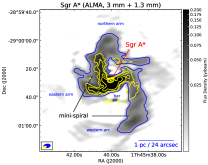
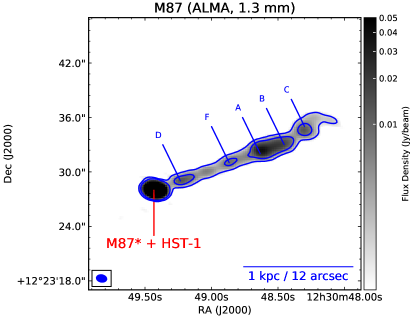
Figure 1: Representative total intensity images. Left panel: Image of Sgr A* at 3 mm on Apr 3 (grey-scale and blue contour) and at 1.3 mm (yellow contours) on Apr 6 2017. The image showcases the well-known “mini-spiral” structure surrounding the central compact core, including the eastern and northern arms, the western arc, and the bar at the center. The contour levels at 1.3 mm are $5\sigma\times 2^{n}$ where $\sigma=$0.44 mJy beam^-1 and n$=0\,,1\,,2\,,3\,\ldots$ up to the peak flux-density; the contour level at 3 mm corresponds to $20\sigma$ ($\sigma=$0.8 mJy beam^-1). The peak flux-density is $2.5\,\pm\,0.1$ ($2.6\,\pm\,0.3$) Jy beam^-1 and the integrated flux density across the entire source is $9.9\,\pm\,0.5$ ($4.9\,\pm\,0.5$) Jy at a representative frequency of 93 (221) GHz. The FOV is given by the primary beam in Band 3 ($\sim$60″) and 1 pc corresponds to 24^′′. The beamsizes are 5$\hbox to0.0pt{.\hss}^{\prime\prime}$0 $\times$ 2$\hbox to0.0pt{.\hss}^{\prime\prime}$7 (P.A.= –81.1^∘) in Band 3 and 2$\hbox to0.0pt{.\hss}^{\prime\prime}$2 $\times$ 1$\hbox to0.0pt{.\hss}^{\prime\prime}$3 (P.A.= -77.5^∘) in Band 6, shown as a blue and yellow ovals, respectively, in the lower left corner. Right panel: Image of M87 at 1.3 mm on Apr 11 2017. The image showcases the structure of the kpc-scale relativistic jet comprised of a bright core at the nucleus and the knots along the jet labeled as D, F, A, B, C; HST-1 is not resolved from the nucleus in these images. The RMS noise level is 0.16 mJy beam^-1, and the contour levels are a factor of 10 and 40 of the RMS. The peak flux-density is 1.34 Jy beam^-1 and the integrated flux-density is 1.57 Jy at a representative frequency of 221 GHz. The FOV is given by the primary beam in Band 6 ($\sim$ 27″ at 1.3 mm). 1 kpc corresponds to 12^′′. This observation was conducted with the most extended array during the VLBI campaign, yielding the highest angular resolution (beam size = 1$\hbox to0.0pt{.\hss}^{\prime\prime}$2 $\times$ 0$\hbox to0.0pt{.\hss}^{\prime\prime}$8, P.A.= 79.3^∘, shown in the lower left corner). In both panels the four observing SPWs (see § 2.1) were used together for imaging. The intensity brightness is plotted using a logarithmic weighting function (starting from the $5\sigma$-level), in order to highlight the full extent of both the mini-spiral (in Sgr A*) and the jet (in M87).

3.1 Representative total intensity images

The sources targeted by the GMVA and EHT are generally unresolved at arcsecond scales and their images are mostly consistent with point sources (see images displayed in Appendix B). The EHT key science targets, Sgr A* and M87, are clear exceptions, and show complex/extended structures across tens of arcseconds. We show representative images of Sgr A* (3 mm, Apr 3; 1.3 mm, Apr 6) and M87 (1.3 mm, Apr 11) in Figure 1. The images displayed cover an area corresponding to the primary beam of the ALMA antennas (27″ in Band 6 and 60″ in Band 3; the correction for the attenuation of the primary beam is not applied to these maps).

The Sgr A* images clearly depict the well-known “mini-spiral” structure which traces ionized gas streams surrounding the central compact source; the mini-spiral has been studied in a wide range of wavelengths (e.g. Zhao et al. 2009; Irons et al. 2012; Roche et al. 2018). The “eastern arm”, the “northern arm”, and the “bar” are clearly seen in both Band 3 and Band 6, while the “western arc” is clearly traced only in the Band 3 image (it falls mostly outside of the antenna primary beam for Band 6). Similar images were obtained in the 100, 250, and 340 GHz bands in ALMA Cycle 0 by Tsuboi et al. (2016, see their Fig. 1). Since Sgr A* shows considerable variability in its core at mm-wavelengths (e.g. Bower et al. 2018), the displayed maps and quoted flux values throughout this paper should be considered as time-averaged images/values at the given epoch.

The M87 jet has been observed across the entire electromagnetic spectrum (e.g., Prieto et al. 2016), and imaged in detail at radio wavelengths from $\lambda$1 metre (with LOFAR: de Gasperin et al. 2012) through $\lambda$[15–0.7] cm (with the VLA and the VLBA: e.g., Hada et al. 2013; Walker et al. 2018) up to $\lambda$ 3 mm (with the GMVA: e.g., Kim et al. 2018). VLA images at lower radio frequencies (e.g., Biretta et al. 1995) showcase a bright component at the nucleus and a kiloparsec-scale (kpc-scale) relativistic jet, extending across approximately 25″ ($\sim 2$ kpc) from the central core. Images of the kpc-scale relativistic jet were also produced with ALMA Cycle-0 observations at $\lambda$ 3 mm (Doi et al. 2013) and with the SMA at $\lambda$ 1 mm (Tan et al. 2008; Kuo et al. 2014), but could only recover the bright central core and the strongest knots along the jet.

Our $\lambda$1.3 mm ALMA image showcases a similar structure, but the higher dynamic range (when compared with these earlier studies) allows us to recover the continuous structure of the straight and narrow kpc-scale jet across approximately 25^′′ from the nucleus, including knots D, F, A, B, C, at increasing distance from the central core (HST-1 is not resolved from the nucleus in these images). The jet structure at larger radii ($\gtrsim 2$ kpc) as well as the jet-inflated radio lobes, imaged in great detail with observations at lower frequencies, are not recovered in our images (see for example the NRAO 20 cm VLA image).

3.2 Extracting Stokes parameters in the compact cores

We extract flux values for Stokes $I$, $Q$, $U$, and $V$ in the compact cores of each target observed in Band 3 and Band 6. We employ three different methods which use both the visibility data and the full-Stokes images. In the $uv$-plane analysis, we use the external casa library uvmultifit (Martí-Vidal et al. 2014). To reduce its processing time, we first average all (240) frequency channels to obtain one-channel four-SPW visibility $uv$-files. We assume that the emission is dominated by a central point source at the phase centre and we fit a delta function to the visibilities to obtain Stokes $I$, $Q$, $U$, and $V$ parameters in each individual SPW. Uncertainties are assessed with Monte Carlo (MC) simulations, as the standard deviation of 1000 MC simulations for each Stokes parameter. For the image-based values, we take the sum of the central nine pixels of the CLEAN model component map (an area of $3\times 3$ pixels, where the pixel size is 0$\hbox to0.0pt{.\hss}^{\prime\prime}$2 in Band 6 and 0$\hbox to0.0pt{.\hss}^{\prime\prime}$5 in Band 3). Summing only the central pixels in the model maps allows one to isolate the core emission from the surroundings in sources with extended structure. A third independent method provides the integrated flux by fitting a Gaussian model to the compact source at the phase-center in each image with the casa task IMFIT. In the remaining of this paper, we will indicate these three methods as uvmf, 3x3, and intf.

From a statistical perspective, any fitting method in the visibility domain should be statistically more reliable than a $\chi^{2}$-based fitting analysis in the image-plane (whose pixels have correlated noise), and should therefore be preferred to image-based methods. However, we have two reasons for considering both approaches in this study: (i) some of our targets exhibit prominent emission structure at arc-second scales (see Figure 1, and the maps in Appendix B), (ii) the observations are carried out with various array configurations, resulting in a different degree of filtering of the source extended emission. Both elements can potentially bias the flux values of the compact cores extracted in the visibility domain vs. the image domain.

In Appendix C we present a comparative analysis of three flux-extraction methods to assess the magnitude of such systematic biases (reported in Table 8). The statistical analysis shows that the Stokes $I$ values estimated with uvmf are consistent with those estimated from the images, with a median absolute deviation (MAD) $\leq 0.07$% and individual offsets $<$1% (for both point sources and extended sources) in the case of the 3x3 method (the agreement is slightly worse for the intf method). These deviations are negligible when compared to the absolute uncertainty of ALMA’s flux calibration (10% in Band 6). This consistency generally holds also for Stokes $Q$ and $U$ (with MAD $<1$%) and other derived parameters within their uncertainties (see Table 8). We therefore conclude that, for the purpose of the polarimetric analysis conducted in this paper, the uv-fitting method uvmf provides sufficiently precise flux values for the Stokes parameters (but see Appendix C for details on M87 and Sgr A*).

Goddi et al. (2019a) report the Stokes $I$ flux values per source estimated in the uv-plane from amplitude gains using the casa task fluxscale. We assess that the Stokes $I$ estimated from the visibilities with uvmf are consistent with those estimated with fluxscale generally within 1%. In addition, Goddi et al. (2019a) compared the fluxscale flux values (after opacity correction) with the predicted values from the regular flux monitoring programme with the ALMA Compact Array (ACA), showing that these values are generally within 10% (see their Appendix B and their Fig. 16). In Appendix D we perform a similar comparative analysis for the sources commonly observed in the ALMA-VLBI campaign and the AMAPOLA polarimetric Grid Survey, concluding that our polarimetric measurements are generally consistent with historic trends of grid sources (see Appendix D for more details and comparison plots).

Table 1: Frequency-averaged polarization properties of GMVA targets (at a representative frequency of 93 GHz).

Source	Day	I	Spectral Index	LP	EVPAa	$\chi_{0}$	RM	Depol.
	[2017]	[Jy]	$\alpha$	[%]	[deg]	[deg]	[$10^{5}$ rad m-2]	[$10^{-4}$ GHz-1]
OJ287	Apr 2	5.97$\pm$0.30	-0.619$\pm$0.029	8.811$\pm$0.030	-70.02$\pm$0.10	-71.85$\pm$0.37	0.0305$\pm$0.0062	2.244$\pm$0.071
J0510+1800	Apr 2	3.11$\pm$0.16	-0.6360$\pm$0.0059	4.173$\pm$0.030	81.86$\pm$0.21	65.49$\pm$0.81	0.273$\pm$0.013	2.639$\pm$0.078
4C 01.28	Apr 2	4.86$\pm$0.24	-0.480$\pm$0.033	4.421$\pm$0.030	-32.27$\pm$0.19	-31.73$\pm$0.74	-0.009$\pm$0.012	2.117$\pm$0.054
Sgr A*	Apr 3	2.52$\pm$0.13	-0.08$\pm$0.13	0.735$\pm$0.030	8.1$\pm$1.4	135.4$\pm$5.3	-2.13$\pm$0.10	4.72$\pm$0.13
J1924-2914	Apr 3	5.11$\pm$0.26	-0.462$\pm$0.026	4.841$\pm$0.030	-46.38$\pm$0.18	-46.68$\pm$0.70	0.005$\pm$0.012	2.34$\pm$0.22
NRAO 530	Apr 3	2.74$\pm$0.14	-0.588$\pm$0.010	0.921$\pm$0.030	38.8$\pm$1.0	51.5$\pm$3.7	-0.213$\pm$0.061	0.4372$\pm$0.0034
4C 09.57	Apr 3	2.85$\pm$0.14	-0.3056$\pm$0.0057	4.069$\pm$0.030	-28.47$\pm$0.21	-31.15$\pm$0.83	0.045$\pm$0.014	0.43$\pm$0.11
3C279	Apr 4	12.93$\pm$0.65	-0.3703$\pm$0.0087	12.159$\pm$0.030	43.906$\pm$0.070	44.98$\pm$0.27	-0.0179$\pm$0.0045	0.456$\pm$0.041
3C273	Apr 4	9.86$\pm$0.49	-0.2887$\pm$0.0049	3.984$\pm$0.030	-45.45$\pm$0.22	-41.87$\pm$0.85	-0.060$\pm$0.014	-2.06$\pm$0.38

Table 2: Frequency-averaged polarization properties of EHT targets (at a representative frequency of 221 GHz).

Source	Day	I	Spectral Index	LP	EVPAa	$\chi_{0}$	RM	Depol.
	[2017]	[Jy]	$\alpha$	[%]	[deg]	[deg]	[$10^{5}$ rad m-2]	[$10^{-4}$ GHz-1]
3C279	Apr 5	8.99$\pm$0.90	-0.642$\pm$0.019	13.210$\pm$0.030	45.180$\pm$0.060	45.20$\pm$0.51	-0.002$\pm$0.048	0.242$\pm$0.051
3C279	Apr 6	9.36$\pm$0.94	-0.619$\pm$0.033	13.010$\pm$0.030	43.340$\pm$0.070	43.41$\pm$0.52	-0.007$\pm$0.049	0.303$\pm$0.018
3C279	Apr 10	8.56$\pm$0.86	-0.6090$\pm$0.0030	14.690$\pm$0.030	40.140$\pm$0.060	40.10$\pm$0.46	0.004$\pm$0.043	0.473$\pm$0.033
3C279	Apr 11	8.16$\pm$0.82	-0.683$\pm$0.019	14.910$\pm$0.030	40.160$\pm$0.060	40.15$\pm$0.46	0.001$\pm$0.043	1.027$\pm$0.015
M87	Apr 5	1.28$\pm$0.13	-1.212$\pm$0.038	2.420$\pm$0.030	-7.79$\pm$0.36	-14.6$\pm$2.8	0.64$\pm$0.27	1.318$\pm$0.031
M87	Apr 6	1.31$\pm$0.13	-1.112$\pm$0.011	2.160$\pm$0.030	-7.60$\pm$0.40	-23.6$\pm$3.1	1.51$\pm$0.30	0.888$\pm$0.046
M87	Apr 10	1.33$\pm$0.13	-1.171$\pm$0.023	2.740$\pm$0.030	0.03$\pm$0.31	2.5$\pm$2.5	-0.24$\pm$0.23	0.540$\pm$0.048
M87	Apr 11	1.34$\pm$0.13	-1.208$\pm$0.019	2.710$\pm$0.030	-0.64$\pm$0.32	3.5$\pm$2.5	-0.39$\pm$0.24	1.553$\pm$0.064
Sgr A*	Apr 6	2.63$\pm$0.26	-0.0270$\pm$0.0030	6.870$\pm$0.030	-65.83$\pm$0.13	-14.7$\pm$1.0	-4.84$\pm$0.10	3.75$\pm$0.10
Sgr A*	Apr 7	2.41$\pm$0.24	-0.057$\pm$0.059	7.230$\pm$0.030	-65.38$\pm$0.12	-18.77$\pm$0.93	-4.412$\pm$0.088	3.33$\pm$0.12
Sgr A*	Apr 11	2.38$\pm$0.24	-0.1450$\pm$0.0080	7.470$\pm$0.030	-49.33$\pm$0.12	-14.66$\pm$0.92	-3.281$\pm$0.087	2.52$\pm$0.32
J1924-2914	Apr 6	3.25$\pm$0.32	-0.780$\pm$0.012	6.090$\pm$0.030	-49.28$\pm$0.14	-53.6$\pm$1.1	0.41$\pm$0.10	0.13$\pm$0.20
J1924-2914	Apr 7	3.15$\pm$0.31	-0.8510$\pm$0.0070	5.970$\pm$0.030	-49.22$\pm$0.15	-52.1$\pm$1.2	0.27$\pm$0.11	0.1470$\pm$0.0080
J1924-2914	Apr 11	3.22$\pm$0.32	-0.677$\pm$0.031	4.870$\pm$0.030	-51.82$\pm$0.18	-56.2$\pm$1.4	0.42$\pm$0.13	0.16$\pm$0.21
OJ287	Apr 5	4.34$\pm$0.43	-0.91$\pm$0.10	9.020$\pm$0.030	-61.190$\pm$0.090	-62.32$\pm$0.73	0.108$\pm$0.069	0.11$\pm$0.63
OJ287	Apr 10	4.22$\pm$0.42	-0.781$\pm$0.088	7.000$\pm$0.030	-61.81$\pm$0.12	-62.6$\pm$1.0	0.077$\pm$0.091	0.09$\pm$0.61
OJ287	Apr 11	4.26$\pm$0.43	-0.715$\pm$0.043	7.150$\pm$0.030	-59.61$\pm$0.12	-62.97$\pm$0.92	0.317$\pm$0.087	0.110$\pm$0.049
4C 01.28	Apr 5	3.51$\pm$0.35	-0.73$\pm$0.16	5.900$\pm$0.030	-23.18$\pm$0.15	-22.5$\pm$1.1	-0.06$\pm$0.11	0.58$\pm$0.20
4C 01.28	Apr 10	3.59$\pm$0.36	-0.679$\pm$0.079	5.080$\pm$0.030	-16.82$\pm$0.17	-16.3$\pm$1.3	-0.05$\pm$0.12	0.68$\pm$0.26
4C 01.28	Apr 11	3.57$\pm$0.36	-0.630$\pm$0.024	5.000$\pm$0.030	-14.74$\pm$0.18	-18.2$\pm$1.4	0.33$\pm$0.13	0.416$\pm$0.054
NRAO 530	Apr 6	1.61$\pm$0.16	-0.96$\pm$0.14	2.350$\pm$0.030	51.59$\pm$0.37	51.7$\pm$2.9	-0.01$\pm$0.28	0.940$\pm$0.062
NRAO 530	Apr 7	1.57$\pm$0.16	-0.812$\pm$0.017	2.430$\pm$0.030	50.67$\pm$0.36	51.1$\pm$2.8	-0.04$\pm$0.27	0.82$\pm$0.15
J0132-1654	Apr 6	0.420$\pm$0.040	-0.625$\pm$0.086	1.990$\pm$0.050	15.54$\pm$0.67	23.4$\pm$5.3	-0.74$\pm$0.50	0.04$\pm$0.40
J0132-1654	Apr 7	0.410$\pm$0.040	-0.75$\pm$0.10	2.010$\pm$0.050	17.85$\pm$0.78	14.3$\pm$6.2	0.34$\pm$0.58	-0.18$\pm$0.21
NGC 1052	Apr 6	0.430$\pm$0.040	-0.83$\pm$0.11	0.120$\pm$0.030	- - - -	- - - -	- - - -	- - - -
NGC 1052	Apr 7	0.380$\pm$0.040	-1.33$\pm$0.16	0.160$\pm$0.040	- - - -	- - - -	- - - -	- - - -
Cen A	Apr 10	5.66$\pm$0.57	-0.197$\pm$0.038	0.070$\pm$0.030	- - - -	- - - -	- - - -	- - - -
3C273	Apr 6	7.56$\pm$0.76	-0.705$\pm$0.024	2.390$\pm$0.030	-55.50$\pm$0.36	-82.2$\pm$2.8	2.52$\pm$0.27	-2.54$\pm$0.11
J0006-0623	Apr 6	1.99$\pm$0.20	-0.789$\pm$0.059	12.530$\pm$0.030	16.480$\pm$0.070	15.83$\pm$0.57	0.061$\pm$0.054	0.78$\pm$0.27

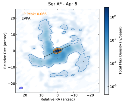
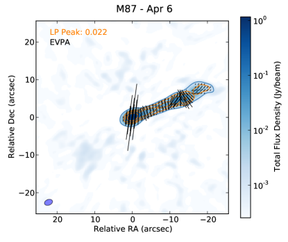
Figure 2: Polarization images of Sgr A* (left panel) and M87 (right panel) at 1.3 mm on Apr 6 2017. The raster image and blue contour show the total intensity emission, the orange contours show the linearly polarized emission, and the black vectors showcase the orientation of the EVPAs (their length is linearly proportional to the polarized flux). The total intensity brightness is plotted using a logarithmic weighting function (starting from the $1\sigma$-level), the blue contour corresponds to $5\sigma$ (where $\sigma$ is the Stokes I map RMS), while the orange contour levels are $5\sigma\times 2^{n}$ (where $\sigma$ is the LP map RMS and n=0,1,2,3… up to the peak in the image). The LP fraction at the peak of the compact core is reported in the upper left corner in each panel. The EVPAs are plotted every 8 pixels (1$\hbox to0.0pt{.\hss}^{\prime\prime}$6 or about 1 per beam) for Sgr A* and every 4 pixels (0$\hbox to0.0pt{.\hss}^{\prime\prime}$8 or about 2 per beam) for M87 (in order to sample more uniformly the jet). According to the measured RM, the EVPAs towards the compact core should be rotated by $-23$^∘ (east of north) in Sgr A* and by $-16$^∘  in M87. The beamsizes (shown as an oval in the lower left corner) are 2$\hbox to0.0pt{.\hss}^{\prime\prime}$2 $\times$ 1$\hbox to0.0pt{.\hss}^{\prime\prime}$3 (P.A. –77^∘) and 2$\hbox to0.0pt{.\hss}^{\prime\prime}$2$\times$1$\hbox to0.0pt{.\hss}^{\prime\prime}$5 (P.A. –69^∘) in the left and right panels, respectively. Note that there are several tiny EVPAs plotted across the mini-spiral, apparently locating regions with polarized flux above the image RMS noise cutoff ($5\sigma$). The LP and EVPA errors are however dominated by the systematic leakage (0.03% of I onto QU), which is not added to the images. Once these systematic errors are added, the LP flux in those points falls below the $3\sigma$ measurement threshold. Therefore we do not claim detection of polarized emission outside of the central core in Sgr A*. Besides, only the polarisation within the inner 1/3 of the primary beam is guaranteed by ALMA. The full set of 1.3 mm observations of Sgr A* and M87 are reported in Figures 8 and 9, respectively.

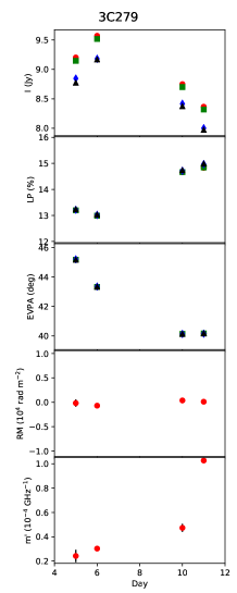
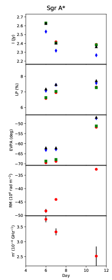
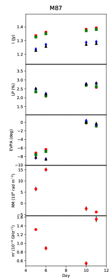
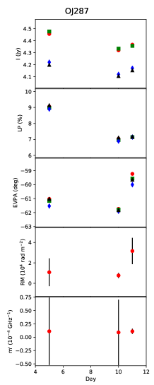
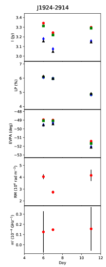
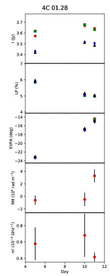
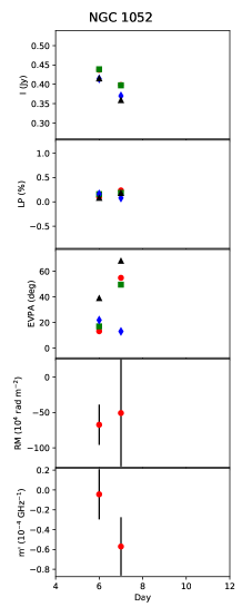
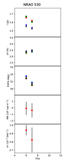
Figure 3: Polarization properties of selected EHT targets observed during the 2017 VLBI campaign as a function of observing day. For each source (labeled at the top of each column), the top panel shows Stokes I (in Jy), the second panel shows the LP degree (in %), the third panel shows the EVPA (in degrees), the fourth panel shows the RM (in units of 10⁴ rad m^-2), and the bottom panel shows the depolarization (in units of 10^-4 GHz^-1). The different symbols and colors in the upper three panels indicate 4 different observing bands centered at 213 GHz (black), 215 GHz (blue), 227 GHz (green), and 229 GHz (red), corresponding to SPW=0,1,2,3. 3C 279 was used as polarization calibrator in all days, except on Apr 7 when J1924-2914 was used.

3.3 Polarimetric data analysis

In this section we use the measured values of the Stokes parameters to determine the polarization properties for all targets, including the fractional LP (§ 3.3.1), the electric vector position angle (EVPA) and its variation as a function of frequency or Faraday Rotation (§ 3.3.2), the degree of depolarization (§ 3.3.3), and the fractional CP (§ 3.3.4). These polarization quantities, averaged across the four SPWs, are reported in Tables 1 and 2 for each target observed with the GMVA and the EHT, respectively (while Table 3 summarizes all the ALMA polarimetric observations towards M87 analysed in this paper). For selected EHT targets, the polarization properties (per SPW and per day) are displayed in Figure 3.

3.3.1 Linear polarization and EVPA

The values estimated for Stokes Q and U can be combined to directly provide the fractional LP in the form $\sqrt{Q^{2}+U^{2}}/I$, as well as the EVPA, $\chi$, via the equation $2\chi=\mathrm{arctan}(U/Q)$. Tables LABEL:tab:GMVA_uvmf_spw and LABEL:tab:EHT_uvmf_spw in Appendix E report Stokes parameters, LP, and EVPA, for each SPW. The LP has been debiased in order to correct for the LP bias in the low SNR regime (this correction is especially relevant for low polarization sources; see Appendix E for the debiased LP derivation).

The estimated LP fractions range from $\lesssim 0.1-0.2$% for the most weakly polarized targets (Cen A and NGC 1052) to 15% for the most strongly polarized target (3C279), consistent with previous measurements (see Appendix D). The uncertainties in LP include the fitting (thermal) error of Stokes $Q$ and $U$ and the (systematic) Stokes $I$ leakage onto Stokes $Q$ and $U$ (0.03% of Stokes $I$) added in quadrature. This analysis yields LP uncertainties $<0.1\%$, similar to those quoted in previous studies (Nagai et al. 2016; Bower et al. 2018).

Figure 2 showcases representative polarization images of Sgr A* (left panel) and M87 (right panel) as observed at 1.3 mm on Apr 6. The individual images display the measured EVPAs overlaid on the polarized flux contour images and the total intensity images. Note that the EVPAs are not Faraday-corrected and that the measured magnetic field orientations should be rotated by 90^∘. In Sgr A*, polarized emission is present only towards the compact core, while none is observed from the mini-spiral. In M87, the EVPA distribution appears quite smooth along the jet, with no evident large fluctuations of the EVPAs in nearby regions, except between Knots A and B. For a negligible RM along the jet, one can infer that the magnetic field orientation is first parallel to the jet axis, then in Knot A it changes direction (tending to be perpendicular to the jet), and then turns back to be parallel in Knot B, and finally becomes perpendicular to the jet axis further downstream (Knot C). This behaviour can be explained if Knot A is a standing or recollimation shock: if multiple standing shocks with different magnetic field configurations form along the jet and the latter is threaded with a helical magnetic field, its helicity (or magnetic pitch) would be different before and after the shock owing to a different radial dependence of the poloidal and toroidal components of the magnetic field (e.g., Mizuno et al. 2015). The EVPA distribution is also in good agreement with the polarization characteristics derived from observations at centimeter wavelengths with the VLA (e.g., Algaba et al. 2016). We nevertheless explicitly note that only the polarisation within the inner third of the primary beam is guaranteed by the ALMA observatory. Since we focus on the polarization properties in the core, the analysis presented in this paper is not affected by this systematics.

3.3.2 Rotation measure

Measuring the EVPA for each SPW (i.e., at four different frequencies) enables us to estimate the RM in the 3 mm band (spanning a 16 GHz frequency range of 85–101 GHz) and in the 1.3 mm band (spanning a 18 GHz frequency range of 212–230 GHz), respectively. In the simplest assumption that the Faraday rotation is caused by a single external Faraday screen (i.e., it occurs outside of the plasma responsible for the polarized emission), a linear dependence is expected between the EVPA and the wavelength squared. In particular, we fit the RM and the mean-wavelength ($\bar{\lambda}$) EVPA ($\bar{\chi}$) following the relation:

$$\chi=\bar{\chi}+RM(\lambda^{2}-\bar{\lambda}^{2})\,,$$ (2)

where $\chi$ is the observed EVPA at wavelength $\lambda$ and $\bar{\chi}$ is the EVPA at wavelength $\bar{\lambda}$. The EVPA extrapolated to zero wavelength (assuming that the $\lambda^{2}$ relation holds) is:

$$\chi_{0}=\bar{\chi}-RM\bar{\lambda}^{2}\,.$$ (3)

The RM fitting is done using a weighted least-squares method of $\chi$ against $\lambda^{2}$. The $\bar{\chi},\ \chi_{0}$, and the fitted RM values are reported in the sixth, seventh, and eighth columns of Tables 1 and 2, respectively.

The EVPA uncertainties quoted in Tables 1, 2, 3, LABEL:tab:GMVA_uvmf_spw, LABEL:tab:EHT_uvmf_spw, are typically dominated by the systematic leakage of 0.03% of Stokes $I$ into Stokes $Q$ and $U$. At 1.3 mm, this results in estimated errors between 0.06^∘ for the most strongly polarized source (3C279) and 0.8^∘ for the weakest source (J0132-1654), with most sources in the range $0.1$^∘– $0.4$^∘. These EVPA uncertainties imply RM propagated errors between $0.4\times 10^{4}$ rad m^-2 and $6\times 10^{4}$ rad m^-2, with most sources in the range $(1-3)\times 10^{4}$ rad m^-2. Similarly, at 3 mm we find EVPA uncertainties of 0.07^∘–1.4^∘, with a typical value of 0.2^∘, and RM uncertainties in the range $(0.06-1.0)\times 10^{4}$ rad m^-2, with a typical value of $\sim 0.13\times 10^{4}$ rad m^-2.

In Appendix F, we present plots of the measured EVPAs at the four ALMA SPWs and their RM fitted models as a function of $\lambda^{2}$ (displayed in Figures 17, 18, 19, and 20) and we discuss the magnitude of thermal and systematic errors in the RM analysis.

3.3.3 Bandwidth depolarization

In the presence of high RM, the large EVPA rotation within the observing frequency bandwidth will decrease the measured fractional polarization owing to Faraday frequency or “bandwidth” depolarization, which depends on the observing frequency band. The RM values inferred in this study (e.g., Table 2) introduce an EVPA rotation of less than one degree within each 2 GHz spectral window, indicating that the bandwidth depolarization in these data should be very low ($<$0.005%). However, if there is an internal component of Faraday rotation (i.e., the emitting plasma is itself causing the RM), there will be much higher frequency-dependent (de)polarization effects (the “differential” Faraday rotation), which will be related to the structure of the Faraday depth across the source (e.g. Cioffi & Jones 1980; Sokoloff et al. 1998).

We have modeled the frequency dependence of LP using a simple linear model:

$$m=\bar{m}+m^{\prime}(\nu-\bar{\nu})\,,$$ (4)

where $m$ is the observed LP at frequency $\nu$, $\bar{m}$ is the LP at the mean frequency $\bar{\nu}$, and $m^{\prime}$ is the change of LP per unit frequency (in GHz^-1). Given the relatively narrow fractional bandwidth ($\lesssim$2 GHz), the linear approximation given in Eq. 4 should suffice to model the frequency depolarization (multifrequency broadband single-dish studies fit more complex models; see for example Pasetto et al. 2016, 2018). We have fitted the values of $m^{\prime}$ from a least-squares fit of Eq. 4 to all sources and epochs, using LP estimates for each spectral window from Table LABEL:tab:EHT_uvmf_spw. We show the fitting results for selected sources in Fig. 3 (lower panels). There are clear detections of $m^{\prime}$ for 3C279, Sgr A*, and M87; these detections also differ between epochs. Such complex time-dependent frequency effects in the polarization intensity may be indicative of an internal contribution to the Faraday effects observed at mm wavelengths.

3.3.4 Circular polarization

Measuring Stokes V provides, in principle, a direct estimate of the fractional CP as $V/I$. In practice, the polarization calibration for ALMA data in CASA is done by solving the polarization equations in the linear approximation, where parallel-hands and cross-hands visibilities are expressed as a linear function of $I$, $Q$, $U$, while it is assumed $V=0$ (e.g., Nagai et al. 2016; Goddi et al. 2019a). A non-negligible Stokes $V$ in the polarization calibrator will introduce a spurious instrumental Stokes $V$ into the visibilities of all the other sources. Moreover, such a Stokes $V$ introduces a bias in the estimate of the cross-polarization phase, $\beta$, at the reference antenna (see Appendix G), which translates into a leakage-like effect in the polconverted VLBI visibilities (see Eq. 13 in Goddi et al. 2019a). The magnitude of such a bias may depend on the fractional CP of the polarization calibrator, the parallactic-angle coverage of the calibrator, and the specifics of the calibration algorithm. In Appendix G we attempt to estimate such a spurious contribution to Stokes $V$ by computing the cross-hands visibilities of the polarization calibrator as a function of parallactic angle (see Figures 21 and 22). This information can then be used to assess Stokes $V$ and CP for all sources in all days (reported in Tables LABEL:tab:GMVA_uvmf_CP and LABEL:tab:EHT_uvmf_CP for GMVA and EHT sources, respectively).

We stress two main points here. First, the reconstructed Stokes $V$ values of the polarization calibrators are non-negligible and are therefore expected to introduce a residual instrumental X–Y phase difference in all other sources, after QA2 calibration. This can be seen in the dependence of the reconstructed Stokes $V$ with feed angle in almost all the observed sources (displayed in Figure 22). The estimated X–Y residual phase offsets are of the order of $0.5^{\circ}$, but they can be as high as $2^{\circ}$ (e.g., on Apr 5). These values would translate to a (purely imaginary) leakage term of the order of a few % in the polconverted VLBI visibilities.

The second point is that there is a significant variation in the estimated values of reconstructed stokes $V$ across the observing week. In particular, on Apr 5, 3C279 shows a much higher value, indicating either an intrinsic change in the source, or systematic errors induced by either the instrument or the calibration. In either case, this anomalously large Stokes $V$ in the polarization calibrator introduces a large X–Y phase difference in all other sources. This can be seen in the strong dependence of reconstructed Stokes $V$ on feed angle for sources OJ287 and 4C 01.28 (displayed in Figure 22, upper left panel) and in their relatively high Stokes $V$ when compared to the following days (see Table LABEL:tab:EHT_uvmf_CP). Besides the anomalous value in Apr 5, it is interesting to note that the data depart from the sinusoidal model described by Eq. G2, for observations far from transit, especially on Apr 11. These deviations may be related to other instrumental effects which however we are not able to precisely quantify. For these reasons, we cannot precisely estimate the magnitude of the true CP fractions for the observed sources (see Appendix G for details). Nevertheless, our analysis still enables us to obtain order-of-magnitude values of CP. In particular, excluding the anomalous Apr 5, we report CP =[–1.0,–1.5] % in Sgr A*, CP$\sim$ 0.3% in M87, and possibly a lower CP level ($\sim 0.1-0.2$%) in a few other AGNs (3C273, OJ287, 4C 01.28, J0132-1654, J0006-0623; see Table LABEL:tab:EHT_uvmf_CP). In the 3 mm band, we do not detect appreciable CP above 0.1%, except for 4C 09.57 (–0.34%), J0510+1800 (–0.14%) and 3C273 (0.14%). We however note that the official accuracy of CP guaranteed by the ALMA observatory is $<$ 0.6% ($1\sigma$) or 1.8% ($3\sigma$), and therefore all of these CP measurements should be regarded as tentative detections.

4 Results

4.1 AGN

We observed a dozen AGN, eight at 3 mm and ten at 1.3 mm (with six observed in both bands), in addition to M87. Following the most prevalent classification scheme found in the literature (e.g. Lister & Homan 2005; Véron-Cetty & Véron 2010), our sample includes three radio galaxies (M87, NGC 1052, Cen A), three BL Lacs (OJ 287, J0006-0623, 4C 09.57), and seven additional QSOs (3C 273, 3C 279, NRAO 530, 4C 01.28, J1924-2914, J0132-1654, and J0510+1800). Following the standard definition of blazar (i.e. an AGN with a relativistic jet nearly directed towards the L.O.S.), we can further combine the last two categories into seven blazars (3C 279, OJ 287, J1924-2914, 4C 01.28, 4C 09.57, J0006-0623, J0510+1800) and three additional QSOs (3C 273, NRAO 530, J0132-1654). The observed radio galaxies have a core that is considered as a LLAGN (e.g., Ho 2008).

Their polarimetric quantities at 3 mm and 1.3 mm are reported in Tables 1 and 2, respectively, and displayed in Figure 3. Overall, we find LP fractions in the range 0.1–15% (with $SNR\sim 3-500\sigma$) and RM in the range $10^{3.3}-10^{5.5}$ rad/m² (with $SNR\sim 3-50\sigma$), in line with previous studies at mm-wavelengths with single-dish telescopes (e.g., Trippe et al. 2010; Agudo et al. 2018) and interferometers (e.g., Plambeck et al. 2014; Martí-Vidal et al. 2015; Hovatta et al. 2019). We also constrain CP to $<$0.3% in all the observed AGN, consistent with previous single-dish (e.g., Thum et al. 2018) and VLBI (e.g., Homan & Lister 2006) studies, suggesting that at mm-wavelengths AGN are not strongly circularly polarized and/or that Faraday conversion of the linearly polarized synchrotron emission is not an efficient process (but see Vitrishchak et al. 2008).

In Appendix B, we also report maps of all the AGN targets observed at 1.3 mm (Figures 10, 11, 12), and at 3 mm (Figure 13), showcasing their arcsecond-structure at mm wavelengths.

In the rest of this section, we briefly comment on the properties of selected AGN.

3C 279

3C 279 is a bright and highly magnetized gamma-ray emitting blazar, whose jet is inclined at a very small viewing angle ($\lesssim 3$^∘). At its distance (z=0.5362), 1 arcsecond subtends 6.5 kpc. 3C 279 was observed on four days at 1.3 mm and one day at 3 mm. It is remarkably highly polarized both at 1.3 mm and 3 mm. At 1.3 mm, LP varies from 13.2% on Apr 5 to 14.9% in Apr 11, while the EVPA goes from 45^∘ down to 40^∘. At 3 mm, LP is slightly lower ($\sim 12.9$%) and the EVPA is 44^∘.

While at 1.3 mm we can only place a $1\sigma$ upper limit of $<$5000 rad/m², at 3 mm we measure a RM$=1790\pm 460$ rad/m² (with a $\sim 4\sigma$ significance). Lee et al. (2015) used the Korean VLBI Network to measure the LP at 13, 7, and 3.5 mm, finding RM values in the range -650 to -2700 rad m^-2, which appear to scale as a function of wavelength as $\lambda^{-2.2}$. These VLBI measurements are not inconsistent with our 3 mm measurement and our upper limits at 1.3 mm, but more accurate measurements at higher frequencies are needed to confirm an increase of the RM with frequency.

The total intensity images at 1.3 mm reveal, besides the bright core, a jet-like feature extending approximately 5^′′ towards south-west (SW) (Fig. 10); such a feature is not discernible in the lower-resolution 3 mm image (Fig. 13). The jet-like feature is oriented at approximately 40^∘, i.e. is roughly aligned with the EVPA in the core. Ultra-high resolution images with the EHT reveal a jet component approximately along the same PA but on angular scales $10^{5}$ times smaller (Kim et al. 2020).

3C 273

3C 273 was the first discovered quasar (Schmidt 1963), and is one of the closest (z=0.158, 1 arcsec = 2.8 kpc) and brightest radio-loud quasars. 3C 273 was observed both at 1.3 mm and 3 mm (2 days apart). Total intensity and LP are higher in the lower frequency band: F=9.9 Jy and LP=4.0% (at 3 mm) vs. F=7.6 Jy and LP=2.4% (1.3 mm). We estimate a RM = $(2.52\pm 0.27)\times 10^{5}$ rad/m² at 1.3 mm, confirming the high RM revealed in previous ALMA observations (conducted in Dec 2016 with 0$\hbox to0.0pt{.\hss}^{\prime\prime}$8 angular resolution) by Hovatta et al. (2019) who report LP=1.8% and a (twice as large) RM$=(5.0\pm 0.3)\times 10^{5}$ rad/m². We also report for the first time a RM measurement at 3 mm, RM = $(-0.60\pm 0.14)\times 10^{4}$ rad/m², about 40 times lower and with opposite sign with respect to the higher frequency band. The $\chi_{0}$ changes from $-82\pm 3$^∘ at 1.3 mm to $-41.9\pm 0.8$^∘ at 3 mm. These large differences may be explained with opacity effects (§ 5.1.1; see also Hovatta et al. 2019). The EVPAs measured at 3 mm and 1.3 mm are in excellent agreement with predictions from the AMAPOLA survey (which however over-predicts LP$\sim$3.5% at 1.3 mm; see Fig. 16).

The total intensity images both at 1.3 mm and 3 mm display, besides the bright core, a bright, one-sided jet extending approximately 20^′′ (54 kpc) to the SW. In the higher resolution 1.3 mm image (Fig. 12), the bright component of the jet is narrow and nearly straight, starts at a separation of $\sim$10^′′ from the core and has a length of $\sim$10^′′. We also detect (at the 3$\sigma$ level) two weak components of the inner jet (within $\sim$10^′′ from the core) joining the bright nucleus to the outer jet. The jet structure is qualitatively similar to previous $\lambda$ cm images made with the VLA at several frequencies between 1.3 and 43 GHz (e.g., Perley & Meisenheimer 2017), where the outer jet appears highly linearly polarized. We do not detect LP in the jet feature.

OJ 287

The bright blazar OJ 287 (z=0.306, 1 arcsec = 4.7 kpc) is among the best candidates for hosting a compact supermassive binary black hole (e.g. Valtonen et al. 2008). OJ287 was observed on three days at 1.3 mm and one day at 3 mm. OJ287 is one of the most highly polarized targets both at 1.3 mm (LP$\sim 7-9$%) and 3 mm (LP = 8.8%). LP drops from 9% on Apr 5 down to 7% on Apr 10, while the EVPA is stable around [-59.6^∘,-61.8^∘] at 1.3 mm and -70^∘  at 3 mm. The LP variation and stable EVPA are consistent with the historical trends derived from the AMAPOLA survey (see Fig. 15). Its flux density is also stable. At 1.3mm, the EVPA either does not follow a $\lambda^{2}$-law (Apr 5 and 11) or the formal fit is consistent with RM = 0 (Apr 10). Although we do not have a RM detection at 1.3 mm, we measure a RM $=3050\pm 620$ rad/m² at 3 mm. A 30 years monitoring of the radio jet in OJ287 has revealed that its (sky-projected) PA varies both at cm and mm wavelengths and follows the modulations of the EVPA at optical wavelengths (Valtonen & Wiik 2012). The observed EVPA/jet-PA trend can be explained with a jet precessing model from the binary black hole which successfully predict an optical EVPA = –66.5^∘ in 2017 (Dey et al., submitted), consistent with actual measurements from optical polarimetric observations during 2016/17 (Valtonen et al. 2017) and close to the EVPA measured at 3 mm and 1.3 mm with ALMA.

NRAO 530

J1733-1304 (alias NRAO 530) is a highly variable QSO (at z = 0.902; 1 arcsec = 8 kpc) that exhibits strong gamma-ray flares. It was observed on two consecutive days at 1.3 mm and one day at 3 mm. It is linearly polarized at a $\sim$2.4% level at 1.3 mm but only 0.9% at 3 mm. The EVPA goes from $\sim 51$^∘ at 1.3 mm to 39^∘ at 3 mm, while $\chi_{0}$ is stable around 51–52^∘. At 3 mm, we estimate RM = $-0.21\pm 0.06\times 10^{5}$ rad/m² at a $3.6\sigma$ significance, which is comparable to the inter-band RM between 1 and 3 mm ($-0.33\times 10^{5}$ rad/m²). These RM values are in agreement with those reported by Bower et al. (2018) at 1.3 mm.

The arcsecond-scale structure at 1.3 mm is dominated by a compact core with a second weaker component at a separation of approximately 10^′′ from the core towards west (Fig. 12). At 3 mm, there is another feature in opposite direction (to the east), which could be a counter jet component (Fig. 13). This geometry is apparently inconsistent with the north-south elongation of the jet revealed on scales $<100$ pc by recent VLBI multi-frequency (22, 43 and 86 GHz) imaging (e.g., Lu et al. 2011), although the Boston University Blazar monitoring program conducted with the VLBA at 7 mm has revealed significant changes in the jet position angle over the years, and possibly jet bending.

J1924-2914

J1924-2914 is a radio-loud blazar at z=0.352 (1 arcsec = 5.1 kpc), which shows strong variability from radio to X-ray. It was observed on three days at 1.3 mm and one day at 3 mm. J1924-2914 appears strongly polarized with LP varying from 6.1% (on Apr 6) to 4.9% (on Apr 11) at 1.3 mm, and LP=4.8% (on Apr 4) at 3 mm. The EVPA is stable around [-49.2^∘,-51.8^∘] at 1.3 mm and -46.4^∘  at 3 mm. We report a RM $\sim([0.3-0.4]\pm 0.1)\times 10^{5}$ rad/m² at 1.3 mm and a $3\sigma$ upper limit of 3600 rad m^-2  at 3 mm (approximately an order of magnitude lower). Bower et al. (2018) report a higher RM value of $(-0.71\pm 0.06)\times 10^{5}$ rad m^-2 at 1.3 mm from ALMA observations carried out in August 2016, when the source LP was considerably lower ($\lesssim 2\%$). The AMAPOLA monitoring revealed a considerable variation in the source EVPA during Mar–Dec 2016, likely due to a period of low LP. We therefore ascribe the difference with the Bower et al. (2018) measurement to source variability.

J1924-2914 is completely unresolved on arcsecond scales both at 1.3 mm and 3 mm (see Figures 11 and 13), a result consistent with images at cm-wavelengths made with the VLA (e.g., Perley 1982).

4C 01.28

J1058+0133 (alias 4C 01.28) is a blazar at z= 0.888 (1 arcsec = 8 kpc). It was observed on three days at 1.3 mm and one day at 3 mm. The source is strongly polarized with a mean LP of 5.5% at 1.3 mm and 4.4% at 3 mm. At 1.3 mm, the LP varies by $<$15% while the EVPA changes from $\sim-23$^∘ (Apr 5) to $\sim-15$^∘ (Apr 11); the EVPA at 3 mm, measured on Apr 2, is –32^∘, apparently consistent with the trend at 1.3 mm. Both the measured EVPA and LP values at 1.3 mm and 3 mm follow very closely the time evolution predicted in the AMAPOLA survey (see Fig. 15), where the LP and EVPA follow a trend parallel to the Stokes $I$ evolution. On Apr 11, we tentatively detect RM $\sim(0.33\pm 0.13)\times 10^{5}$ rad m^-2 at the $\sim 3\sigma$ level; we however caution that on Apr 5 and 10 the EVPAs do not follow the $\lambda^{2}$ trend (Fig. 17), and we do not have a RM detection at 3 mm (with a $3\sigma$ upper limit of 3600 rad m^-2).

Cen A

Centaurus A (Cen A) is the closest radio-loud AGN (at a distance of 3.8 Mpc, 1 arcsec = 18 pc). Although it is a bright mm source (with F=5.7 Jy), it is unpolarized at 1.3 mm (with a $3\sigma$ LP upper limit of 0.09%). We find a spectral index of –0.2 in the central core, consistent with a flat spectrum, as also measured between 350 and 698 GHz with (non-simultaneous) ALMA observations (Espada et al. 2017).

The total intensity images reveal a diffuse emission component around the central bright core, extending across 12″ and mostly elongated north-south, and two additional compact components towards north-east (NE) separated by roughly 14″ and 18″ from the central core and aligned at P.A.$\sim$50^∘ (see Fig. 12, bottom-right panel). The first component could be associated with the inner circumnuclear disk, mapped in CO with the SMA (Espada et al. 2009) and ALMA (Espada et al. 2017), and may indicate the presence of a dusty torus. The two additional components correspond to two knots of the northern lobe of the relativistic jet, labelled as A1 (inner) and A2 (outer) in a VLA study by Clarke et al. (1992); no portion of the southern jet is seen, consistent with previous observations (McCoy et al. 2017).

NGC 1052

NGC 1052 is a nearby (19.7 Mpc; 1 arcsec = 95 pc) radio-galaxy that showcases an exceptionally bright twin-jet system with a large viewing angle close to 90 degrees (e.g., Baczko et al. 2016). With F$\sim$0.4 Jy and LP$<$0.15%, it is the weakest mm source (along with J0132-1654) and the second least polarized AGN in our sample. The apparent discrepancy in flux-density and spectral index between Apr 6 and 7 is most likely a consequence of the low flux-density (below the threshold required by the commissioned on-source phasing mode; see § 2.2) and the much poorer data quality on Apr 7, rather than time-variability of the source.

Remaining AGN

J0006-0623 is the most highly polarized blazar (after 3C279) observed at 1.3 mm, with LP = 12.5%. J0132-1654 is the weakest QSO observed at 1.3 mm ($F\sim$0.4 Jy) and has LP$\sim 2$%. The blazar J0510+1800 has an LP $\sim$ 4% at 3 mm and shows indication of a large RM ($\sim 0.27\times 10^{5}\,$rad/m²), although the EVPA distribution does not follow a $\lambda^{2}-$dependence (see Fig. 19, upper-right panel).

4.2 M87

We report the first unambiguous measurement of RM toward the M87 nucleus at mm wavelengths (Table 2; Figure 17, middle panels). We measure $(1.51\pm 0.30)\times 10^{5}$ rad m^-2 (with a $5\sigma$ significance) on Apr 6 and tentatively $(0.64\pm 0.27)\times 10^{5}$ rad m^-2 (with a $2.4\sigma$ significance) on Apr 5. On the last two days we can only report best-fit values of $(-0.24\pm 0.23)\times 10^{5}$ rad m^-2 (with a $3\sigma$ confidence level range $[-0.93,0.45]$) on Apr 10 and $(-0.39\pm 0.24)\times 10^{5}$ rad m^-2 (with a $3\sigma$ confidence level range $[-1.11,0.33]$) on Apr 11. Although we cannot determine precisely the RM value on all days, we can conclude that the RM appears to vary substantially across days and there is marginal evidence of sign reversal.

Before this study, the only RM measurement was done with the SMA at 230 GHz by Kuo et al. (2014), who reported a best-fit RM = $(-2.1\pm 1.8)\times 10^{5}$ rad m^-2  ($1\sigma$ uncertainty) and could therefore only provide an upper limit. In order to better constrain the RM amplitude and its time variability, in addition to the 2017 VLBI observations (which are the focus of this paper), we have also analysed the ALMA data acquired during the Apr 2018 VLBI campaign as well as additional ALMA archival polarimetric experiments (these are introduced in §2.4). For two projects (2016.1.00415.S and 2017.1.00608.S) we produced fully-calibrated $uv$-files and then used the uvmf flux extraction method with uvmultifit to determine the M87 Stokes parameters. For the remaining two projects (2013.1.01022.S and 2015.1.01170.S), we used the full-Stokes images released with QA2. Since these images do not include clean component models, we used the intf  method to extract the Stokes parameters in the compact core directly in the images.

Table 3 reports the full list of ALMA observations, project codes, and derived polarimetric parameters. In total, we have collected data from three and eight different observations at 3 mm and 1.3 mm, respectively, spanning three years (from Sep 2015 to Sep 2018). The main findings revealed by the analysis of the full dataset are the following:

1. The total flux density is quite stable on a week timescale, varying by $\lesssim$5% in both Apr 2017 and Apr 2018, and exhibiting total excursion of about 15-20% across one year both at 1.3 mm (decreasing from Apr 2017 to Apr 2018) and 3 mm (increasing from Sep 2015 to Oct 2016).

2. We detect LP $\sim$ 1.7–2.7% (2.3% mean; Apr 2017 – Apr 2018) at 1.3 mm and LP $\sim$ 1.3–2.4% (1.7% mean; Sep 2015 – Oct 2016) at 3 mm.

3. The EVPA distributions across the four ALMA SPWs clearly display a $\lambda^{2}$ dependence, on specific dates, within both the 1.3 mm and 3 mm bands (e.g., see Figures 17 and 20).

4. The magnitude of the RM varies both at 3 mm (range $|\rm{RM}|=[0.2-1.2]\times 10^{5}$ rad m^-2) and 1.3 mm (range $|\rm{RM}|=[1.5-4.1]\times 10^{5}$ rad m^-2, including $<3\sigma$ non-detections).

5. The RM can either be positive or negative in both bands (with a preference for a negative sign), indicating that sign flips are present both at 3 mm and 1.3 mm.

6. In Apr 2017, the RM magnitude appears to vary significantly (from non-detection up to 1.5 $\times$ $10^{5}$ rad m^-2) in just 4–5 days.

7. In Apr 2017, $\chi_{0}$ varies substantially across a week, being [$-14.6\pm 2.8,\ -23.6\pm 3.1,\ 2.5\pm 2.5,\ 3.5\pm 2.5$] in Apr 5, 6, 10, and 11, respectively. Therefore, although the EVPA at 1.3 mm changes only by $\sim$+8^∘ during the observing week, the $\chi_{0}$ varies by -9^∘ in the first two days, and +27^∘ between the second day and the last two days. In Apr 2018 $\chi_{0}$ appears instead to be consistently around 68.4^∘–70.6^∘. The $\chi_{0}$ derived from the three 3 mm experiments (Sep, Nov 2015 and Oct 2016) spans a range from $\sim$4^∘ to 107^∘ (see Fig. 4 for a summary plot of RM+$\chi_{0}$ in all the available M87 observations).

8. The EVPAs measured at 1.3 mm in the 2017 campaign ($\sim[-8,0]$^∘) are significantly different to the ones measured in the 2018 campaign ($\sim[26,36]$^∘), which are instead consistent with the ones measured in 2015–2016 at 3 mm ($\sim[21,33]$^∘).

9. We find hints of CP at 1.3 mm at the $[-0.3\pm 0.6,-0.4\pm 0.6]$% level, but these should be regarded as tentative measurements (see also Appendix G for caveats on the CP estimates).

We will interpret these findings in Section 5.2.

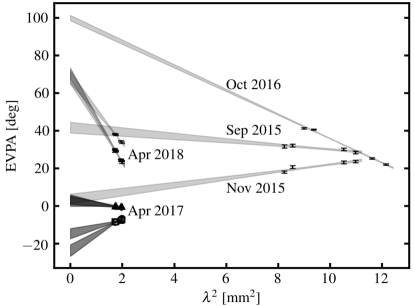
Figure 4: M87 EVPA as a function of $\lambda^{2}$ observed in multiple epochs at 3 mm (from Sep 2015 to Nov 2016) and 1.3 mm (from Apr 2017 to Apr 2018). Each grey line is a linear fit to the EVPAs measured at the four ALMA Band 3 and Band 6 SPW, yielding the RM in each epoch, and the extrapolated intercept at the Y-axis is $\chi_{0}$. Note the large offset in $\chi_{0}$ between the 3 mm and 1.3 mm bands.

4.3 Sgr A*

In this section, we analyse the polarimetric properties of Sgr A* and its variability on a week timescale based on the ALMA observations at 1.3 mm and 3 mm.

LP.

We measured LP between 6.9% and 7.5% across one week at 1.3 mm (Table 2). These values are broadly consistent with historic measurements using BIMA on several epochs in the time span 2002–2004 at 227 GHz (7.8–9.4%; Bower et al. 2003, 2005), SMA on several days in Jun–Jul 2005 (4.5–6.9% at 225 GHz; Marrone et al. 2007), and more recently with ALMA in Mar–Aug 2016 at 225 GHz (3.7–6.3%, 5.9% mean; Bower et al. 2018, who also report intra-day variability). Besides observations at 1.3 mm, LP variability has been reported also at 3.5 mm with BIMA (on a timescale of days– Macquart et al. 2006) and at 0.85 mm with the SMA (on a timescale from hours to days– Marrone et al. 2006). All together, these measurements imply significant time-variability of LP across timescales of hours/days to months/years.

While at 1.3 mm LP $\sim$ 7%, at 3 mm we detect LP $\lesssim$ 1% (Table 1). It is interesting to note that the LP fraction increases from $\sim$ 0.5% at $\sim$ 86 GHz (our SPW=0,1) up to $\sim$ 1% at $\sim$ 100 GHz (our SPW=2,3; see Table LABEL:tab:GMVA_uvmf_spw). This trend is consistent with earlier measurements at 22 GHz and 43 GHz with the VLA, and at 86 GHz and 112–115 GHz with BIMA, yielding upper limits of LP$\sim$ 0.2, 0.4%, 1% (Bower et al. 1999b), and 1.8% (Bower et al. 2001), respectively (but see Macquart et al. 2006, who report LP $\sim$ 2% at 85 GHz with BIMA observations in Mar 2004).

RM.

We report a mean RM of $-4.2\times 10^{5}$ rad m^-2  at 1.3 mm with a significance of $\sim 50\sigma$ (Table 2; Figure 17, upper second to fourth panels), consistent with measurements over the past 15 years since the first measurements with BIMA+JCMT (Bower et al. 2003), BIMA+JCMT+SMA (Macquart et al. 2006), and the SMA alone (Marrone et al. 2007). Across the observing week, we see a change in RM from $-4.84\pm 0.1\times 10^{5}$ rad m^-2  (on Apr 6) to $-3.28\pm 0.09\times 10^{5}$ rad m^-2  (on Apr 11), corresponding to a change of $\sim-1.5\times 10^{5}$ rad m^-2  ($\sim$30%), detected with a significance of $\sim 20\sigma$. This RM change can completely explain the EVPA variation from –65.8^∘$\pm$0.1^∘ to –49.3^∘$\pm$0.1^∘ (or a $\sim$16^∘ change across 5 days), given the consistency in $\chi_{0}$ between Apr 6 and Apr 11 ($\sim-14.7$^∘$\pm 1.0$^∘; see Table 2). Marrone et al. (2007) find a comparable dispersion based on six measurements in the time period Jun–Jul 2005 ($\Delta|{\rm RM}|=1.3\times 10^{5}$ rad m^-2  excluding their most discrepant point, or $\Delta|{\rm RM}|=3.8\times 10^{5}$ rad m^-2  including all 6 measurements spanning almost 2 months). Bower et al. (2018) find an even larger $\Delta|{\rm RM}|=-4.9\times 10^{5}$ rad m^-2  across 5 months; they also report intra-day variability in a similar range on timescales of several hours.

Variations in RM appear to be coupled with LP fraction: the lower the polarization flux density, the higher the absolute value of the RM. In particular, we find $\Delta{\rm LP}\sim+5\%$ ($\Delta{\rm RM}\sim-9\%$) and $\Delta{\rm LP}\sim+9$% ($\Delta{\rm RM}\sim-32\%$) in Apr 7 and 11, respectively, with respect to Apr 6. This can be understood if a larger RM scrambles more effectively the polarization vector fields resulting in lower net polarization. Although with only three data points we cannot draw a statistically significant conclusion, we note that the same trend was also seen by Bower et al. (2018) on shorter (intra-day) timescales.

We report for the first time a measurement of RM at 3 mm, with a magnitude of $(-2.1\pm 0.1)\times 10^{5}$ rad m^-2 (Table 1; Figure 17, upper-left panel). The RM magnitude at 3 mm (measured on Apr 3) is a factor of 2.3 (2.1) smaller than the RM value measured at 1.3 mm on Apr 6 (Apr 7). Furthermore, we note a large offset in $\chi_{0}$ between the 3 mm (+135^∘  or –45^∘ for a full 180^∘ wrap) and the 1.3 mm bands ($\sim[-14.7,-18.8]$^∘), which is unlikely a consequence of time variability (given the $\chi_{0}$ consistency on Apr 6–11). The comparison of RM and $\chi_{0}$ in the two frequency bands (showcased in Fig. 5) indicates the presence of both Faraday and intrinsic changes of the source. We will provide an interpretation of the differences observed between the two frequency bands in § 5.3.

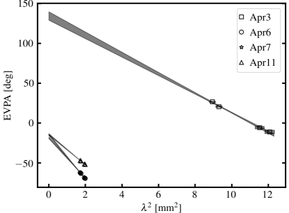
Figure 5: Sgr A* EVPA as a function of $\lambda^{2}$ observed in 2017 at 3 mm (Apr 3) and 1.3 mm (Apr 6, 7, 11). Each grey line is a linear fit to the EVPAs measured at the four ALMA Band 3 and Band 6 SPWs, yielding the RM in each epoch, and the extrapolated intercept at the Y-axis is $\chi_{0}$. Note the large offset in $\chi_{0}$ between the 3 mm and 1.3 mm bands, despite the consistency of $\chi_{0}$ at 1.3 mm across 6 days.

CP.

We report a tentative detection of CP at 1.3 mm in the range $(-1.0\pm 0.6)$% to $(-1.5\pm 0.6)$%. This is consistent with the first detection with the SMA from observations carried out in 2005–2007 (Muñoz et al. 2012) and with a more recent ALMA study based on 2016 observations (Bower et al. 2018). This result suggests that the handedness of the mm-wavelength CP is stable over timescales larger than 12 yr. Interestingly, historical VLA data (from 1981 to 1999) between 1.4 and 15 GHz show that the emission is circularly polarized at the 0.3% level and is consistently left-handed (Bower et al. 1999a, 2002), possibly extending the stability of the CP sign to 40 years. Such a remarkable consistency of the sign of CP over (potentially four) decades suggests a stable magnetic field configuration (in the emission and conversion region).

Similarly to the RM, we also note a weak anti-correlation between LP and CP (although more observations are needed to confirm it).

We do not detect CP at 3 mm ($<0.06\%$, $3\sigma$ upper limit). Muñoz et al. (2012) and Bower et al. (2018) find that, once one combines the cm and mm measurements, the CP fraction as a function of frequency should be characterized by a power law with $\nu^{0.35}$. Using the measurements at 1.3 mm, this shallow power-law would imply a CP fraction at the level of $\sim 0.7-1.1$% at 3 mm, which would have been readily observable. The non detection of CP at 3 mm suggests that the CP spectrum may not be monotonic.

Although the origin of the CP is not well understood, since a relativistic synchrotron plasma is expected to produce little CP, Muñoz et al. (2012) suggest that the observed CP is likely generated close to the event horizon by the Faraday conversion which transforms LP into CP via thermal electrons that are mixed with the relativistic electrons responsible for the linearly polarized synchrotron emission (Beckert & Falcke 2002). In this scenario, while the high degree of order in the magnetic field necessary to produce LP $\sim$ 7% at 1.3 mm naturally leads to a high CP in a synchrotron source, the absence of CP at 3 mm is consistent with the low LP measured. See Muñoz et al. (2012) for a detailed discussion of potential origins for the CP emission.

A final caveat is that based on the analysis presented in §3.3.4 and Appendix G, the physical interpretations above should be considered as tentative.

Flux-density variability

We do not report significant variability in total intensity and polarized intensity, which is about 10% in six days (comparable to the absolute flux-scale uncertainty in ALMA Band 6). Marrone et al. (2006) and Bower et al. (2018) report more significant variability in all polarization parameters based on intra-day light curves in all four Stokes parameters. This type of analysis is beyond the scope of this paper, and will be investigated elsewhere.

Table 3: M87 RM measurements with ALMA.

Date	I	LP	EVPA	$\chi_{0}$	RM	Beamsize	Project Code
	[Jy]	[%]	[deg]	[deg]	[$10^{5}$ rad m-2]
3 mm
2015/09/19	2.17$\pm$0.11	1.37$\pm$ 0.03	30.68$\pm$0.74	41.7$\pm$3.1	-0.201$\pm$0.054	0$\hbox to0.0pt{.\hss}^{\prime\prime}$53	2013.1.01022.S
2015/11/11	1.93$\pm$0.10	1.30$\pm$ 0.03	21.47$\pm$0.69	3.9$\pm$2.7	0.318$\pm$0.049	0$\hbox to0.0pt{.\hss}^{\prime\prime}$15	2015.1.01170.Sa
2016/10/04	1.85$\pm$0.10	2.39$\pm$0.03	33.35$\pm$0.36	107.4$\pm$1.4	-1.227$\pm$0.023	0$\hbox to0.0pt{.\hss}^{\prime\prime}$43	2016.1.00415.S
1.3 mm
2017/04/05	1.28$\pm$0.13	2.42$\pm$ 0.03	-7.78$\pm$0.37	-14.6$\pm$2.9	0.64$\pm$0.27	1$\hbox to0.0pt{.\hss}^{\prime\prime}$5	2016.1.01154.V
2017/04/06	1.31$\pm$0.13	2.16$\pm$ 0.03	-7.61$\pm$0.39	-23.6$\pm$3.1	1.51$\pm$0.29	1$\hbox to0.0pt{.\hss}^{\prime\prime}$8	2016.1.01154.V
2017/04/10	1.33$\pm$0.13	2.74$\pm$ 0.03	0.11$\pm$0.32	3.5$\pm$2.5	-0.32$\pm$0.24	1$\hbox to0.0pt{.\hss}^{\prime\prime}$5	2016.1.01154.V
2017/04/11	1.31$\pm$0.13	2.71$\pm$ 0.03	-0.63$\pm$0.31	3.7$\pm$2.4	-0.41$\pm$0.23	1$\hbox to0.0pt{.\hss}^{\prime\prime}$0	2016.1.01154.V
2018/04/21	1.11$\pm$0.11	2.29$\pm$ 0.03	27.18$\pm$0.38	70.6$\pm$3.0	-4.11$\pm$0.28	0$\hbox to0.0pt{.\hss}^{\prime\prime}$9	2017.1.00841.V
2018/04/22	1.18$\pm$0.12	1.71$\pm$ 0.03	26.42$\pm$0.52	68.9$\pm$4.0	-4.02$\pm$0.39	0$\hbox to0.0pt{.\hss}^{\prime\prime}$9	2017.1.00841.V
2018/04/25	1.14$\pm$0.11	2.21$\pm$ 0.03	36.12$\pm$0.39	68.4$\pm$3.0	-3.05$\pm$0.29	0$\hbox to0.0pt{.\hss}^{\prime\prime}$9	2017.1.00841.V
2018/09/25	1.16$\pm$0.12	0.78$\pm$ 0.04	–	–	–	0$\hbox to0.0pt{.\hss}^{\prime\prime}$35	2017.1.00608.S

5 Discussion

In this section, we review general polarization properties of AGN comparing the two (1.3 mm and 3 mm) frequency bands, different AGN classes, and depolarization mechanisms (§ 5.1); then we interpret the Faraday properties derived for M87 in the context of existing accretion and jet models as well as a new two-component polarization model (§ 5.2); and finally we discuss additional constraints on the Sgr A* polarization model from a comparison of 1.3 mm and 3 mm observations (§ 5.3).

5.1 Polarization degree and Faraday rotation in AGN

5.1.1 1.3 mm vs. 3 mm

Synchrotron emission opacity

The total intensity spectral indexes for the AGN sources in the sample vary in the range $\alpha$=[–0.7,–0.3] at 3 mm and $\alpha$=[–1.3,–0.6] at 1.3 mm, Cen A being the only exception, with $\alpha$=–0.2 (see Tables 1 and 2 and Appendix H). This contrasts with the flat spectra ($\alpha$=0) typically found at longer cm wavelengths in AGN cores (e.g., Hovatta et al. 2014), corresponding to optically-thick emission. In addition, we observe a spectral steepening (with $\Delta\alpha=[-0.2,-0.4]$) between 3 mm and 1.3 mm; although one should keep in mind the caveat of time variability, since the observations in the two frequency bands were close in time (within ten days) but not simultaneous. Such spectral steepening can naturally be explained by decreased opacity of the synchrotron emission at higher frequencies in a standard jet model (e.g., Blandford & Königl 1979; Lobanov 1998).

LP degree

We detect LP in the range 0.9–13% at 3 mm and 2–15% at 1.3 mm (excluding the unpolarized sources NGC 1052 and Cen A). At 1.3 mm, the median fractional polarization is 5.1%, just slightly higher than the median LP at 3 mm, 4.2%, yielding a ratio of 1.2. If we consider only the sources observed in both bands, then the ratio goes slightly up to 1.3 (or 1.6 including also Sgr A*). Despite the low statistics, these trends are marginally consistent with results from previous single-dish surveys with the IRAM 30-m telescope (Agudo et al. 2014, 2018) and the Plateau de Bure Interferometer or PdBI (Trippe et al. 2010). In particular, Agudo et al. (2014) find an LP ratio of 1.6 between 1 mm and 3 mm based on simultaneous, single-epoch observations of a sample of 22 radio-loud ($F>1$ Jy) AGN, while Agudo et al. (2018) find an LP ratio of 2.6 based on long-term monitoring, non-simultaneous observations of 29 AGN. Trippe et al. (2010) find similar numbers from a sample of 73 AGN observed as part of the IRAM/PdBI calibration measurements during standard interferometer science operations. The comparison of these statistics at both wavelengths suggests a general higher degree of polarization at 1 mm as compared to 3 mm. This finding can be related either to a smaller size of the emitting region and/or to a higher ordering of the magnetic-field configuration (e.g., see discussion in Hughes 1991). In fact, according to the standard jet model, the size of the core region decreases as a power-law of the observing frequency, which could help explain the higher LP observed at 1 mm. Alternatively, the more ordered magnetic-field configuration could be related to a large-scale (helical) magnetic-field structure along the jets.

Faraday RM

Among the six sources observed both at 3 mm and 1.3 mm, we have RM detections at the two bands only in 3C273, where the estimated value at 3 mm is significantly lower than at 1.3 mm. For the remaining sources with RM detections at 3 mm (NRAO 530, OJ 287, and 3C279) and at 1.3 mm (J1924-2914 and 4C 01.28), their $3\sigma$ upper limits, respectively at 1.3 mm and 3 mm, still allow a larger RM at the higher frequency band.

A different ’in-band’ RM in the 3 mm and 1.3 mm bands can be explained either with (i) the presence of an internal Faraday screen or multiple external screens in the beam; or with (ii) a different opacity of the synchrotron emission between the two bands. Case (i) will cause a non-$\lambda^{2}$ behaviour of the EVPA and a non-trivial relation between the ’in-band’ RM determined at only two narrow radio bands. Evidence for non-$\lambda^{2}$ behaviour of the EVPA can be possibly seen in OJ 287, 4C 01.28, and J0006-0623 at 1.3 mm (Fig. 18) and J0510+1800 at 3 mm (Fig. 19). In order to estimate $B$ or $n_{e}$ from the RM (see Eq. 1), one would need to sample densely the EVPA over a broader frequency range and perform a more sophisticated analysis, using techniques like the Faraday RM synthesis or Faraday tomography (e.g. Brentjens & de Bruyn 2005). This type of analysis is beyond the scope of this paper and can be investigated in a future study (we refer to § 5.2.1 for evidence of internal Faraday rotation and § 5.2.2 for an example of a multiple component Faraday model for the case of M87). Since the spectral index analysis shows that the AGN in the sample become more optically thin at 1 mm, the observed differences in the ’in-band’ RM at 3 mm and 1.3 mm can be likely explained with synchrotron opacity effects alone (with the caveat of time variability since the observations are near-in-time but not simultaneous).

It is also interesting to note that we also see a sign reversal between the RM measured at 3 mm and 1.3 mm for 3C 273. RM sign reversals require reversals in $B_{||}$ either over time (the observations in the two bands were not simultaneous) or across the emitting region (the orientation of the magnetic field is different in the 3 mm and 1 mm regions). With the data in hand we cannot distinguish between time variability or spatial incoherence of the magnetic field (we refer to § 5.2 for a discussion on possible origins of RM sign reversals in AGN).

5.1.2 Blazars vs. other AGN

We find that blazars are more strongly polarized than other AGN in our sample, with a median LP $\sim$7.1% vs. 2.4% at 1.3 mm, respectively. Furthermore, blazars have approximately an order-of-magnitude lower RM values (on average) than other AGN, with a median value of $\sim 0.07\times 10^{5}$ rad m^-2  at 1.3 mm (with the highest values of $\sim 0.4\times 10^{5}$ rad m^-2 exhibited by J1924-2914), whereas for other AGN we find a median value of $\sim 0.4\times 10^{5}$ at 1.3 mm (with the highest values $>10^{5}$ rad m^-2  exhibited by M87 and 3C 273).

Bower et al. (2017) used the Combined Array for Millimeter Astronomy (CARMA) and the SMA to observe at 1.3 mm two low-luminosity AGN (LLAGN), M81 and M84, finding upper limits to LP of 1%–2%. Similarly, Plambeck et al. (2014) used CARMA to observe the LLAGN 3C 84 at 1.3 and 0.9 mm, measuring an LP in the 1%–2% range, and a very high RM of $\sim(9\pm 2)\times 10^{5}$. These low values of LP (and high values of RM) are comparable to what we find in M87, which is also classified as a LLAGN (e.g. Di Matteo et al. 2003).

When put together, these results suggest that blazars have different polarization properties at mm wavelengths from all other AGN, including LLAGN, radio galaxies, or regular QSOs. These mm polarization differences can be understood in the context of the viewing angle unification scheme of AGN. A smaller viewing angle implies a stronger Doppler-boosting of the synchrotron emitting plasma in the jet, which in turn implies a higher polarization fraction for blazars. Furthermore, their face-on geometry allows the observer to reach the innermost radii of the nucleus/jet and reduces the impact of the ‘scrambling’ of linearly polarized radiation by averaging different polarization components within the source (e.g. Faraday and beam depolarization – see next section), also resulting in higher LP (and lower RM).

5.1.3 Depolarization in radio galaxies

In the previous section we point out that radio galaxies and LLAGN exhibit lower polarization degree than blazars. In particular, the radio galaxies Cen A and NGC 1052 do not show appreciable polarized intensity (LP$<$0.2%) at 1.3 mm. We suggest several depolarization mechanisms that may be at play in these radio galaxies (and potentially other LLAGN):

1. Faraday depolarization due to a thick torus or a dense accretion flow.

2. Bandwidth depolarization due to a strong magnetic field.

3. Beam depolarization due to a disordered magnetic field.

4. Thermal (non-synchrotron) emission.

In the following, we elaborate on these mechanisms.

a. Faraday depolarization due to a thick torus or a dense accretion flow

Radio galaxies are often surrounded by an obscuring torus. The cold gas in the torus can be photo-ionized by UV photons from the inner accretion disk and the mixture of thermal and non-thermal material could be responsible for the strong depolarization of the inner regions via Faraday rotation – and one speaks of Faraday depolarization. In the case of NGC 1052, Fromm et al. (2018, 2019) created synthetic radio maps of the jets using special-relativistic hydrodynamic (SRHD) simulations and suggested that an obscuring torus can explain some of the observed properties of these jets. In fact, the presence of a massive ($\sim 10^{7}\,M_{\odot}$) and dense ($>10^{7}$ cm^-3) molecular torus has been recently demonstrated with ALMA observations (Kameno et al. 2020). A clumpy torus is also known to surround the nucleus of Cen A (e.g. Espada et al. 2017), as also suggested by our 1.3 mm map (see Fig. 12, bottom-right panel). Therefore the presence of a thick torus of cold gas could naturally explain the low polarization degree in both radio galaxies. A similar mechanism can be at play in LLAGN whose radio emission is thought to be powered by synchrotron radiation from a geometrically thick, hot accretion flow (e.g., Narayan & Yi 1994; Blandford & Begelman 1999; Quataert & Gruzinov 2000).

b. Bandwidth depolarization due to a strong magnetic field

A large homogeneous magnetic field implies an intrinsically large homogeneous RM (see Eq. 1), resulting in the source to appear unpolarized in broadband observations – and one speaks of bandwidth depolarization. In NGC 1052, GMVA imaging at 86 GHz helped constrain the magnetic field at Schwarzschild radius ($R_{Sch}$) scales in the range 360–70000 G (Baczko et al. 2016), providing evidence of an extremely high magnetic field near the SMBH. Coupled with its high inclination (e.g. Kadler et al. 2004), such a strong magnetic field would result in the source to appear unpolarized in ALMA broadband observations.

c. Beam depolarization due to a tangled magnetic field

If the magnetic field in the emitting regions or in a foreground Faraday screen is tangled or generally disordered on scales much smaller than the observing beam, magnetic field regions with similar polarization degrees but opposite signs will cancel out and the net observed polarization degree would be significantly decreased – and one speaks of beam depolarization. We do not have evidence of such tangled magnetic field for any of the low LP sources in our sample, which will require high-resolution polarization imaging with the GMVA or the EHT.

d. Thermal (non-synchrotron) emission

Multi-wavelength (MWL) studies in Cen A show that its SED is moderately inverted up to the infrared, possibly indicating a dust contribution at mm wavelengths (e.g. Espada et al. 2017). Using VLBI imaging at 229 GHz with the EHT, Janssen et al. (submitted) measured a flux of $\sim 2$ Jy in the VLBI core, indicating that the EHT filters out $\sim 65$% of the emission seen by ALMA. While we cannot exclude contribution from thermal emission to the total flux measured by ALMA, the flux measured with the EHT must necessarily be associated with non-thermal emission. We therefore conclude that dust emission is an unlikely explanation for the lack of LP at 1.3 mm.

An improved data analysis including spectro-polarimetry could be helpful to measure the actual RM in both NGC 1052 and Cen A and thus assess which is the dominant depolarization mechanism among the ones discussed above (this is however beyond the scope of this paper). As a final note, an interesting insight may come from a comparison between mm and IR wavelengths, where both NGC 1052 (Fernández-Ontiveros et al. 2019) and Cen A (Jones 2000; Lopez Rodriguez 2021) are highly polarized. These characteristic are similar to Cygnus A, where the low polarized core at mm-wavelengths and the high polarized core at IR wavelengths may be the signature of an ordered magnetic field in the plane of the accretion disk supporting the accretion flow and/or jet formation (Lopez-Rodriguez et al. 2018).

5.2 Physical origin of the rotation measure in M87

We can now use the polarimetric and Faraday properties of the mm emission from M87 reported in § 4.2, to constrain properties of accretion models onto the M87 SMBH. Models aiming to explain the origin of the RM in M87 should match the following key observed features (see § 4.2 for a full list of findings):

1. Low LP and high RM. M87 has a rather low LP ($\sim 2.3\%$ mean at 1.3 mm) when compared to Sgr A* and other blazars in the sample (see §5.1.2), while the measured RM can be as high as a few times $10^{5}$ rad m^-2.

2. RM sign reversals. Observations on different dates yield large differences in the measured RM values, which can be either positive or negative (in both the 3 mm and 1.3 mm bands). This requires sign flips in $B_{||}$ over time and/or across the emitting region.

3. Rapid RM time variability. In Apr 2017, the RM magnitude appears to vary significantly (from non-detection up to $1.5\times 10^{5}$ rad m^-2) in just 4-5 days. This suggests the presence of small-scale fluctuations in the emitting source and/or the Faraday screen.

4. $\lambda^{2}$ scaling. Plots in Figures 17 and 20 clearly display a $\lambda^{2}$ dependence of the EVPA at 1.3 mm and 3 mm on specific days (although this is not always the case).

The MWL spectral energy distribution (SED) of the M87 core is best explained by emission from advection dominated/radiatively inefficient accretion flow (ADAF/RIAF – Reynolds et al. 1996; Di Matteo et al. 2003) or from a jet (e.g., Dexter et al. 2012; Prieto et al. 2016; Mościbrodzka 2019), or emission from a combination of these two components (e.g., Broderick & Loeb 2009; Nemmen et al. 2014; Mościbrodzka et al. 2016; Feng et al. 2016; Mościbrodzka et al. 2017; Davelaar et al. 2019; Event Horizon Telescope Collaboration et al. 2019e). In the hybrid models, the low-frequency radio emission is produced by the jet while the optically-thin mm/submm (and X-ray) emission can either come from the jet base or the inner accretion flow.

The traditional approach adopted in previous studies was to assume that the large scale ($r\sim~{}100$ $R_{Sch}$) accretion flow itself may act as a Faraday screen and that the core emission region lies entirely behind the same portion of the Faraday screen (e.g., the core emission size is small compared to the scale of any fluctuations in large scale flow). In the framework of semi-analytic RIAF/ADAF models, the RM magnitude has then been used to estimate mass accretion rates onto black holes in Sgr A* (Marrone et al. 2006, 2007) and in 3C 84 (Plambeck et al. 2014). A similar approach has been used in M87, yielding estimates of the accretion rate in the range from $\dot{M}<9\times 10^{-4}$ (Kuo et al. 2014) to $\dot{M}\sim[0.2,1]\times 10^{-3}$ $M_{\odot}$ yr^-1(Feng et al. 2016), where the quoted values are either upper limits or depend on specific model assumptions (e.g. black hole spin or the exact location of the Faraday screen). From the largest RM that we measured, $4\times 10^{5}$ rad m^-2 (on Apr 2018), using Equation (9) in Marrone et al. (2006), we would infer a mass accretion rate of $\dot{M}=7.7\times 10^{-8}|RM|^{2/3}\sim 4\times 10^{-4}$ $M_{\odot}$ yr^-1 assuming an inner boundary to the Faraday screen of $R_{\rm RM,in}=21$ $R_{Sch}$ (as suggested by Kuo et al. 2014).

While our estimates of mass accretion rates are consistent with previous similar estimates and upper limits from the ADAF/RIAF models, the observed properties listed above, especially the time variable RM and its sign reversals, provide new constraints. In particular, the timescale of the RM variability can be set by the rotating medium dynamical time ($\propto\sqrt{R^{3}/GM}$), thus constraining the radius at which the RM originates. The rapid variability observed in Apr 2017 implies that the RM should occur much closer to the SMBH (within a few $R_{Sch}$) than assumed in previous mass accretion models, which in turn suggests the possibility of a co-location of the emitting and rotating medium. In the alternative, the Faraday screen could be at further distance and the observed variability could be ascribed to rapid fluctuations in the emitting source. Therefore, both a turbulent accretion flow acting as a Faraday screen or a varying compact source with an external screen can explain the observed time-variability. Finally, the accretion flow is not the only possible source of Faraday rotation. Since simulations show that relativistic jets can have a “spine-sheath” structure (e.g., McKinney 2006), the jet sheath can provide a magnetized screen surrounding the jet, and indeed it has been also suggested as a plausible source of Faraday rotation in AGN (e.g., Zavala & Taylor 2004). Therefore, either (or both) the accretion flow and/or the jet can in principle be the sources of the mm emission and/or the Faraday rotation.

All the scenarios described above imply a more complicated physical origin of the Faraday rotation than is usually assumed in traditional semi-analytic models that use the RM to infer a mass accretion rate. We conclude that, unlike the case of Sgr A*, the RM in M87 may not provide an accurate estimate of the mass accretion rate onto the black hole.

In what follows, we review clues on the location of the Faraday screen using observational constrains from ALMA (§ 5.2.1) as well as information on horizon scales from the EHT (§ 5.2.2).

5.2.1 Location of the Faraday screen: internal vs. external

We distinguish between two general cases: internal and external Faraday rotation.

1. Internal Faraday rotation: the accretion flow or jet can simultaneously be the source of synchrotron radiation and the Faraday screen.

   1. RM rapid time variability and sign reversals. Recent time-dependent GRMHD simulations of the M87 core (Ricarte et al. 2020) show that turbulence within the accretion flow is able to change $B_{||}$ in both amplitude and orientation, resulting in significant RM fluctuations and sign reversals on the dynamical time at $R\simeq 2.5-5$ $R_{Sch}$, corresponding to short timescales of a few days for M87 (consistent with properties #ii and #iii).

   2. Beam Depolarization. An internal Faraday screen could cause beam depolarization of the synchrotron emission. This has been theoretically predicted by GRMHD simulations of the M87 core emission, which yield low values of LP (typically in the range 1%—3%) and large Faraday RM ($\gtrsim 10^{5}$ rad m^-2) (Mościbrodzka et al. 2017; Event Horizon Telescope Collaboration et al. 2021b), broadly consistent with the observed feature #i. We however note that the beam depolarization could be also caused by external Faraday rotation in an inhomogeneous screen.

2. External Faraday rotation: the emission region lies entirely behind (and it is not inter-mixed with) the Faraday screen.

   1. $\lambda^{2}$ scaling of the EVPA. A $\lambda^{2}$ dependence is typically adopted as observational evidence of the fundamental assumption on the location of the Faraday screen as external relative to the background source. Although it can be argued that EVPA variations in a narrow frequency range could be approximated to be linear (at 1.3/3 mm the fractional $\lambda^{2}$ bandwidth is only 16/32% of the central wavelength), good linear fits of EVPA vs. $\lambda^{2}$ are also obtained from lower-frequency observations, including the range 2, 5 and 8 GHz (Park et al. 2019), 8, 15, 22 and 43 GHz (Algaba et al. 2016), and 24, 43 and 86 GHz (Kravchenko et al. 2020).

   2. RM sign reversals and helical magnetic fields. Polarimetric images with the VLBA at 43 GHz have revealed magnetic field vectors wrapped around the core (Walker et al. 2018), suggesting that toroidal fields might be dominant on scales of hundreds of $R_{Sch}$. Helical magnetic fields threading the jet may be produced by the differential rotation either in the BH ergosphere or in the innermost regions of the accretion disk (e.g., Broderick & Loeb 2009; Broderick & McKinney 2010; Tchekhovskoy et al. 2011). If toroidal fields are dominant in the sheath, one would expect transverse RM gradients across the jet, with opposite signs of the RM from one edge to the other, as shown in a handful cases where VLBI images resolve the jet width ( e.g., Asada et al. 2002; Gómez et al. 2008; Gabuzda et al. 2014). Systematic changes in the signs of these gradients, leading to RM sign reversals in unresolved measurements, can be explained with a number of models, including the magnetic ”tower” model (Lynden-Bell 1996; Contopoulos & Kazanas 1998; Lico et al. 2017), or the ”striped” jet model (Parfrey et al. 2015; Mahlmann et al. 2020; Nathanail et al. 2020). Nevertheless, it remains difficult to explain the rapid fluctuations observed in Apr 2017 with these models.

A long-term monitoring with beam-matched simultaneous observations at multiple frequency bands would be required to assess the frequency-dependence of the RM and to conclusively discriminate between internal and external Faraday rotation. Clear evidence of $\lambda^{2}$ scaling in a wider frequency range would be evidence of the external scenario, while deviations from $\lambda^{2}$ would support the internal scenario. A time cadence from a few days to a few months would allow us to assess whether the RM sign flips are stochastic (favoring the internal scenario), or systematic (favoring the external scenario).

5.2.2 Two-component polarization model for M87

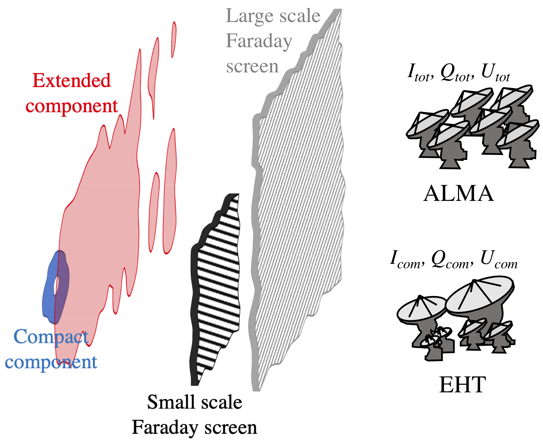
Figure 6: Diagram of the two-component model, comprised of a compact (blue) and extended (red) polarized emission regions with corresponding small-scale and large-scale Faraday screens. The small-screen, which may be external (shown) or internal (not shown) acts only on the compact component, which is observed by the EHT. ALMA observes the combined emission from both components.

EHT estimates of the flux in the compact core, i.e., that arising on horizon scales, can at most account for $50\%$ of that measured by ALMA, both in total intensity (Event Horizon Telescope Collaboration et al. 2019d) and polarized intensity (Event Horizon Telescope Collaboration et al. 2021a) emission. Natural origins for the additional emission are the larger-scale structures in the jet. The additional components may encompass many scales, be discrete features (e.g., HST-1), or be a combination thereof. In order to interpret these differences revealed by the EHT and ALMA, we adopt the simplest version of a multi-scale model permissible – a two-component model comprised of a variable compact region and static extended region (see Figure 6). We find that this is sufficient to harmonize the polarimetric properties observed by both the EHT and ALMA in Apr 2017, including the interday variability in the ALMA RMs and the EVPA variation of the compact core as observed by the EHT.

Both the compact and extended components of the two-component model consist of total intensity, spectral index, linearly polarized flux, and polarization angle. We consider both internal and external Faraday screen models for the compact component. In both cases, the Faraday screen for the extended component is assumed to be external. A model likelihood is constructed using the integrated EHT Stokes $I$, $Q$, and $U$ ranges presented in Table 7 in Appendix H2 of Event Horizon Telescope Collaboration et al. (2021a), and the ALMA core Stokes $I$, $Q$, and $U$ values for the individual SPWs in Table LABEL:tab:EHT_uvmf_spw, assuming Gaussian errors. This likelihood is then sampled with the EMCEE python package (Foreman-Mackey et al. 2013) to obtain posterior probability distributions for the model components. For more details regarding the model, priors, and fit results, see Appendix I.

Across days, only the LP and EVPA of the compact component is permitted to vary. This is consistent with the extended component being associated with much larger physical structures and required by the polarimetric variability observed by the EHT (Event Horizon Telescope Collaboration et al. 2021a). There is no evidence that variability in any other component of the two-component model is required: despite static Faraday screens, permitting the polarization of the compact component to vary is capable of reproducing the rapid changes in the ALMA RMs. In this picture, the observed RMs arise in part from the wavelength-dependent competition between the two components, and thus are not directly indicative of the properties of either Faraday screen.

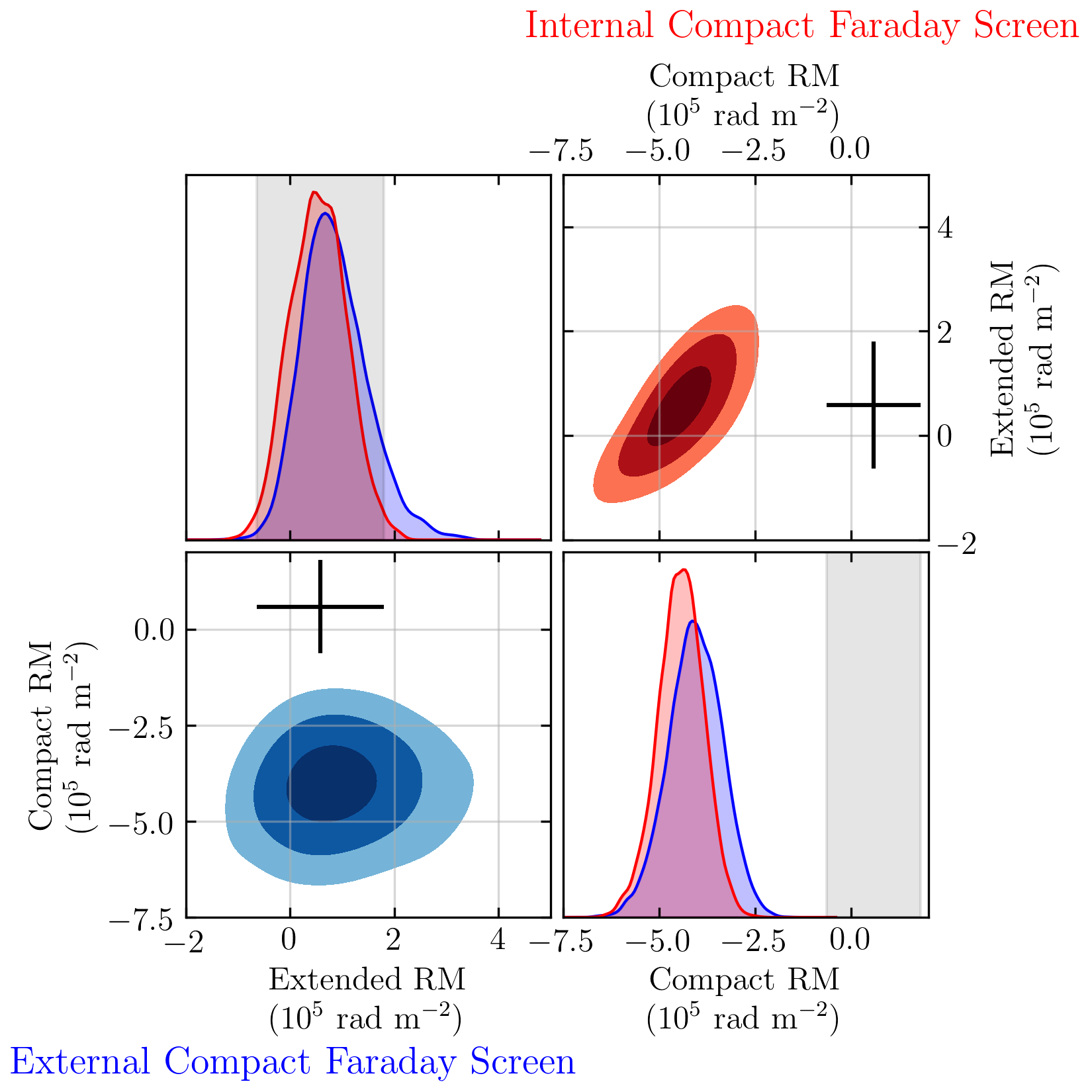
Figure 7: Posteriors implied by the April 5, 6, 10, and 11, 2017 ALMA and EHT observations for the RMs measured on ALMA (extended) and EHT (compact) scales in the two component model when it is assumed that the compact Faraday screen is external (lower left, blue) and internal (upper right, red) to the emission region. Contours are shown for the 50%, 90%, and 99% quantiles. For comparison, the $2\sigma$ range of April 5, 6, 10, and 11, 2017 ALMA RMs reported in Table 3 are shown by the black crosses and gray bands.

Nevertheless, via this model we are able to separately constrain the RMs that are observed on ALMA and EHT scales; these are shown in Figure 7. Specifically, while the RM of the large-scale Faraday screen is comparable to the Apr 2017 values reported in Table 3, that associated with the compact component is not directly constrained by the ALMA measurements and can be factors of many larger: at 95% confidence, the compact RM is between $-5.4\times 10^{5}~{}{\rm rad~{}m^{-2}}$ and $-2.9\times 10^{5}~{}{\rm rad~{}m^{-2}}$. Interestingly, the estimated range is consistent with the RM inferred from low-inclination GRMHD models of the M87 core (Ricarte et al. 2020; Event Horizon Telescope Collaboration et al. 2021b) and comparable to the Apr 2018 values reported in Table 3. This consistency suggests the possibility that in Apr 2018 ALMA may be seeing the core RM (e.g., as a consequence of a different beating of the two components). This hypothesis can be directly tested with the 2018 EHT observations which, unlike the 2017 ones, covered the full frequency spacing of ALMA (212–230 GHZ; see § 2.1), and are therefore expected to directly measure the resolved RM of the core. This will in turn allow to quantify the interplay between compact and extended components, and potentially explain the time variability observed with ALMA.

5.3 Constraints on Sgr A* model from polarization and Faraday properties at 3 mm and 1.3 mm

Measurements of Faraday rotation at radio/mm wavelengths, either towards Sgr A* itself (e.g., Marrone et al. 2007; Bower et al. 2018) or the nearby pulsar PSR J1745-2900 (e.g., Eatough et al. 2013; Kravchenko et al. 2016), have been used to probe the magnetized accretion flow in Sgr A* on scales from tens of $R_{Sch}$ out to the Bondi radius ($\sim 10^{5}$ $R_{Sch}$). Using the same semi-analytic RIAF/ADAF models introduced in § 5.2 (Marrone et al. 2006), from the measured RM values at 1.3 mm we obtain an accretion rate of order $10^{-8}$ $M_{\odot}$ yr^-1 (assuming $R_{\rm RM,in}=10$ $R_{Sch}$), with a maximum variation of approximately 20% across the observing week.

We have derived for the first time the polarization and Faraday properties of Sgr A* both at 3 mm and 1.3 mm in a time-window of ten days. Since the synchrotron photosphere in the accretion flow moves outwards with decreasing frequency (because of increased opacity), the polarized emission at 3 mm and 1.3 mm is expected to arise from different locations with potentially different magnetic field structures. Any variation of the intrinsic EVPA or RM with frequency can therefore provide interesting insights on the polarized source and magnetic field structure. In § 4.3 we infer that the intrinsic polarization vector is rotated between the 3 mm ($\chi_{o}\sim+135$^∘  or –45^∘ assuming a full 180^∘ wrap) and the 1.3 mm ($\chi_{o}\sim$ [–15^∘,–19^∘]) bands and that the RM magnitude at 3 mm is about half of the RM value measured at 1.3 mm over a three-days separation. From earlier VLBI measurements, we know that the emission at mm wavelengths must come from very closely situated regions of the black hole, with an intrinsic (i.e. unscattered) size of $\sim$120 $\mu$as (or 12 $R_{Sch}$) at 3.5 mm (Issaoun et al. 2019) and $\sim$50 $\mu$as (or 5 $R_{Sch}$) at 1.3 mm (Lu et al. 2018). Therefore the radius of the 3.5 mm source is 2.4 times larger than the 1.3 mm source, i.e. very close to the ratio of the RM values measured with ALMA at the two wavelengths (see RM paragraph in § 4.3). Taken at face value, this result suggests that about half of the Faraday rotation at 1.3 mm may occur between the 3 mm photosphere and the 1.3 mm source.

Although this result would be extremely constraining for the model of Sgr A*, we should point out two caveats: i) possible presence of multiple components; ii) potential RM time variability. We explain these caveats below.

Multiple components

In addition to the mini-spiral, which is however unpolarized (see § 3.3.1) and thus should not contribute significantly to the polarized flux, the presence of a relativistic compact jet has been proposed based on theoretical modeling of the source SED, in particular to explain the radio emission in Sgr A* (e.g., Falcke & Markoff 2000). In addition, the only available VLBI polarimetry study at 1.3 mm has shown that the polarization structure of Sgr A* is complex (Johnson et al. 2015) and can be in principle different at the two wavelengths. Therefore, we cannot completely exclude the presence of an additional jet component to the accretion flow or a more complex morphology for the intrinsic polarization. Nevertheless, we argue that the stability of LP, RM, and CP (including their sign) observed in Sgr A* over more than a decade, unlike the case of M87, favors the presence of one single dominating polarized component.

RM time variability

At 1.3 mm, the RM changes by $+1.5\times 10^{5}$ rad/m² ($\sim$ 30%) between the Apr 6/7 and Apr 11. Assuming the same rate of time variability at 3 mm and 1.3 mm, such variability is likely not responsible for a factor of two difference over three days. Likewise, the large offset in $\chi_{o}$ observed at 3 mm and 1.3 mm is unlikely a consequence of time variability, given the $\chi_{0}$ consistency on Apr 6–11. Larger variations in RM were however recorded by Marrone et al. (2007) and Bower et al. (2018) on timescales from hours to months (see for example Figure 12 in Bower et al. 2018). Since the observations in the two frequency bands were close in time but not simultaneous, we cannot definitely exclude time variability as the origin of the observed difference in RM magnitude at 3 mm and 1.3 mm.

Future simultaneous measurements over a wider wavelength range (including 3 mm and 1.3 mm) will allow us to separate time variability and source structure effects.

6 Conclusions

We have determined and analysed the polarization and Faraday properties of Sgr A*, the nucleus of M87, and a dozen radio-loud AGN, observed with ALMA during the 2017 VLBI campaign in the 3 mm and 1 mm bands in concert with the GMVA and the EHT, respectively.

Our main findings can be summarised as follows:

1. The AGN sources in our sample are highly polarized, with linear polarization degrees in the range 2–15% at 1.3 mm and 0.9–13% at 3 mm. The radio galaxies NGC 1052 and Cen A are the only exceptions with LP$<$0.2%.

2. The AGN sources have negative spectral indexes varying in the range $\alpha=[-1.3,-0.2]$, in contrast with the flat spectra ($\alpha$=0) typically found at longer cm wavelengths in AGN cores. We also observe a spectral steepening between the 3 mm and the 1.3 mm bands, which can naturally be explained by decreased opacity of the synchrotron emission at higher frequencies in a standard jet model (e.g., Lobanov 1998).

3. We find marginal evidence for a general higher degree of polarization and RM magnitude in the 1 mm band as compared to the 3 mm band (a trend which is consistent with single-dish surveys). The increase of polarized intensity at higher frequency may be the result of an increased magnetic-field order in the inner portions of jets and/or to the smaller size of the high-frequency emitting regions. The increase of RM with frequency can be explained by opacity effects: emission at higher frequencies is generated in, and propagates along, regions with higher magnetic fields and plasma densities (e.g. Hovatta et al. 2014). Given the small-number statistics (eight AGN observed at 3 mm, eleven at 1.3 mm, and six in both bands) and the caveat of time variability (in a time window of ten days), simultaneous observations of a larger AGN sample at multiple frequency bands are needed to confirm these results.

4. The blazars (seven in our sample) have on average the highest level of polarization (LP $\sim$7.1% at 1.3 mm) and an order of magnitude lower RM ($\sim 0.07\times 10^{5}$ rad m^-2  at 1.3 mm) when compared with other AGN in our sample (with LP $\sim$2.4% and RM $\sim 0.4\times 10^{5}$ rad m^-2, respectively). These mm polarization differences can be understood in the context of the viewing angle unification scheme of AGN: blazars’ face-on geometry implies a stronger Doppler-boosting of the synchrotron emitting plasma in the jet and reduces the effect of Faraday and beam depolarization in the accretion flow, resulting in higher LP (and lower RM). Future observations of a broader sample of sources are necessary for assessing the statistical significance of these trends.

5. We constrain the circular polarization fraction in the observed AGN to $<$0.3%. For Sgr A* we report CP = [-1.0,-1.5]%, consistent with previous SMA and ALMA studies. However, we explicitly note that the ALMA observatory does not guarantee a CP level $<$0.6% ($1\sigma$), therefore these measurements should be regarded as tentative detections.

6. We derive for the first time the polarization and Faraday properties of Sgr A* both at 3 mm and 1.3 mm in a time-window of ten days. The RM magnitude at 3 mm, $(-2.1\pm 0.1)\times 10^{5}$ rad/m², is about half of the RM value measured at 1.3 mm over a three-days separation, suggesting that about half of the Faraday rotation at 1.3 mm may occur between the 3 mm photosphere and the 1.3 mm source (although we cannot exclude effects related to time variability).

7. We report the first unambiguous measurement of Faraday rotation toward the M87 nucleus at mm wavelengths. At variance with Sgr A*, the M87 RM exhibits significant changes in magnitude and sign reversals. At 1.3 mm, it spans from positive values ($+1.5\times 10^{5}$ rad m^-2 at a $5\sigma$ level), to $<3\sigma$ non-detections in Apr 2017, to negative values ($-3$ to $-4\times 10^{5}$ rad m^-2 at a $10\sigma$ level) in Apr 2018. At 3 mm the RM measured values span the range from $-1.2\rm\ to\ 0.3\times 10^{5}$ rad m^-2 from Sep 2015 to Oct 2016. The large scatter and time variability revealed by the ALMA measurements suggest a more complicated physical origin of the Faraday rotation than is usually assumed in models using the RM to infer a mass accretion rate. We conclude that, unlike the case of Sgr A*, the RM in M87 may not provide an accurate estimate of the mass accretion rate onto the black hole.

8. The observed RM in M87 may result from Faraday rotation internal to the emission region, as commonly found in GRMHD models of turbulent accretion flows or expected in a structured jet, or from a time-varying helical magnetic field threading the jet boundary layer acting as an external Faraday screen. As an alternative, we put forward a two-component model comprised of a variable compact region and static extended region. We find that this simple model is able to simultaneously explain the polarimetric properties observed in Apr 2017 by both the EHT (on horizon scales) and ALMA (which observes the combined emission from both components).

The ALMA measurements presented in this work provide critical constraints for the calibration and analysis of simultaneously obtained VLBI data. This is an essential resource for two instruments like the EHT and the GMVA which have the resolving power to reveal polarization structures and measure magnetic field strengths and particle densities on horizon scales (in the case of M87 and Sgr A*) and/or in the inner few parsecs for the AGN.

Table 4: Projects and sources observed in the 3 mm Band.

Date	Project	Target	Pol. Cal.	Other sources	UT range
2017 Apr 02	2016.1.01116.V	OJ287	4C 01.28	J0510+1800	06:55:08 – 15:19:43
2017 Apr 03	2016.1.00413.V	Sgr A*	NRAO 530	J1924–2914, 4C 09.57	20:52:28 – 04:43:54
2017 Apr 04	2016.1.01216.V	3C273	3C279	—	00:24:57 – 05:32:46

Table 5: Projects and sources observed in the 1.3 mm Band.

Date	Project	Target	Pol. Cal.	Other sources	UT range
2017 Apr 05					04/22:12 – 05/09:13
	2016.1.01114.V	OJ287	3C279	4C 01.28, M87	04/22:12 – 05/03:22
	2016.1.01154.V	M87	3C279	4C 01.28, OJ287	05/03:24 – 05/07:18
	2016.1.01176.V	3C279	3C279	M87	05/07:19 – 05/09:13
2017 Apr 06					06/00:18 – 06/16:19
	2016.1.01154.V	M87	3C279	3C273	06/00:18 – 06/08:02
	2016.1.01404.V	Sgr A*	3C279	NRAO 530, J1924–2914	06/08:03 – 06/14:40
	2016.1.01290.V	NGC 1052	3C279	J0132-1654, J0006-0623	06/14:51 – 06/16:19
2017 Apr 07					07/03:45 – 07/20:47
	2016.1.01404.V	Sgr A*	J1924–2914	NRAO 530	07/03:45 – 07/14:31
	2016.1.01290.V	NGC 1052	J1924–2914	J0132-1654, 3C 84a	07/19:23 – 07/20:47
				J0006-0623a
2017 Apr 10					09/23:02 – 10/10:02
	2016.1.01114.V	OJ287	3C279	4C 01.28, M87	09/23:02 – 10/03:49
	2016.1.01176.V	3C279	3C279	Cen A, M87	10/03:51 – 10/06:21
	2016.1.01198.V	Cen A	3C279	—	10/06:23 – 10/10:02
2017 Apr 11					10/21:44 – 11/10:31
	2016.1.01114.V	OJ287	3C279	4C 01.28	10/21:44 – 11/00:22
	2016.1.01154.V	M87	3C279	—	11/00:23 – 11/05:03
	2016.1.01176.V	3C279	3C279	M87	11/05:05 – 11/08:45
	2016.1.01404.V	Sgr A*	3C279	J1924–2914	11/08:46 – 11/14:03

Appendix A Projects observed during the 2017 VLBI campaign

Tables 4 and 5 list the projects observed in the 3 mm and 1.3 mm bands, ordered by date of execution. Each row reports the observing date, the ALMA project code, the science target, the source used as polarization calibrator, other sources observed in the project, and the duration of each observation. In Table 5, each row-group refers to an individual VLBI run or ”Track”, which includes observations of different projects carried out during the same night. The calibration of EHT projects was done per track (and not per project; see Goddi et al. 2019a). Two sources listed in Table 5, 3C 84 and J0006-0623, both observed on Apr 07, were excluded from the analysis presented in this paper: 3C 84 was observed with an elevation below 25^∘, while J0006-0623 was observed for just $\sim 2$ min close to an elevation of 25^∘; the resulting calibrated data display critical phase and amplitude scatter and hence were flagged before data analysis (see § 2.2).

Table 6: Frequency-averaged imaging parameters of GMVA sources (at a representative frequency of 93 GHz).

Source	T${}_{\rm on\ source}$	RMS(I)	RMS(Q)	RMS(U)	RMS(V)	Synthesized Beam
	[h]	[mJy]	[mJy]	[mJy]	[mJy]	$\theta_{M}$[′′] $\times\theta_{m}$[′′] (P.A.[∘])
Apr 2
OJ287	2.584	0.31	0.34	0.46	0.17	4.7 ′′ $\times$ 2.7′′ (-86.2∘)
4C 01.28	0.269	0.17	0.30	0.36	0.14	4.9 ′′ $\times$ 2.4′′ (-86.8∘)
J0510+1800	0.363	0.31	0.29	0.52	0.12	5.8 ′′ $\times$ 2.5′′ (-70.1∘)
Apr 3
J1924-2914	0.270	0.16	0.65	0.13	0.13	5.5 ′′ $\times$ 2.5′′ (-75.2∘)
NRAO 530	0.479	0.02	0.02	0.02	0.03	4.8 ′′ $\times$ 2.4′′ (-83.5∘)
Sgr A*	2.643	0.80	0.09	0.08	0.04	5.0 ′′ $\times$ 2.7′′ (-81.1∘)
4C 09.57	0.133	0.09	0.08	0.14	0.07	6.1 ′′ $\times$ 2.7′′ (72.0∘)
Apr 4
3C273	1.396	0.48	0.26	0.54	0.13	5.0 ′′ $\times$ 3.4′′ (-86.7∘)
3C279	0.215	0.37	0.20	0.15	0.18	5.0 ′′ $\times$ 3.4′′ (-85.8∘)

Table 7: Frequency-averaged imaging parameters of EHT sources (at a representative frequency of 221 GHz).

Source	Ton-source	RMS(I)	RMS(Q)	RMS(U)	RMS(V)	Synthesized Beam
	[h]	[mJy]	[mJy]	[mJy]	[mJy]	$\theta_{M}$[′′] $\times\theta_{m}$[′′] (P.A.[∘])
Apr 5
M87	1.645	0.18	0.05	0.05	0.02	2.0 ′′ $\times$ 1.0′′ (-85.5∘)
3C279	1.068	0.24	0.09	0.07	0.16	2.2 ′′ $\times$ 0.9′′ (-80.9∘)
OJ287	1.406	0.13	0.16	0.15	0.11	2.0 ′′ $\times$ 1.1′′ (88.7∘)
4C 01.28	0.230	0.12	0.11	0.08	0.12	2.0 ′′ $\times$ 0.9′′ (87.0∘)
Apr 6
J0006-0623	0.045	0.47	0.12	0.15	0.13	2.2 ′′ $\times$ 1.4′′ (-81.1∘)
J0132-1654	0.059	0.06	0.06	0.06	0.06	2.3 ′′ $\times$ 1.4′′ (87.8∘)
NGC 1052	0.373	0.05	0.03	0.03	0.03	2.7 ′′ $\times$ 1.3′′ (80.3∘)
Sgr A*	2.529	0.44	0.18	0.33	0.08	2.2 ′′ $\times$ 1.3′′ (-77.5∘)
J1924-2914	0.269	0.10	0.07	0.08	0.11	2.2 ′′ $\times$ 1.3′′ (-82.5∘)
NRAO 530	0.269	0.04	0.06	0.05	0.05	2.2 ′′ $\times$ 1.3′′ (-76.4∘)
M87	1.613	0.24	0.06	0.06	0.02	2.2 ′′ $\times$ 1.5′′ (-69.4∘)
3C279	0.430	0.30	0.13	0.08	0.13	2.2 ′′ $\times$ 1.3′′ (-78.4∘)
3C273	0.403	0.19	0.10	0.09	0.10	2.3 ′′ $\times$ 1.4′′ (-75.0∘)
Apr 7
NGC 1052	0.200	0.11	0.04	0.04	0.04	2.6 ′′ $\times$ 1.0′′ (-76.3∘)
J0132-1654	0.056	0.08	0.07	0.07	0.06	3.0 ′′ $\times$ 1.0′′ (-72.8∘)
NRAO 530	0.403	0.08	0.03	0.03	0.05	2.1 ′′ $\times$ 0.9′′ (-89.6∘)
J1924-2914	0.312	0.18	0.04	0.04	0.08	2.1 ′′ $\times$ 0.9′′ (89.7∘)
Sgr A*	4.109	0.25	0.14	0.13	0.04	2.1 ′′ $\times$ 0.9′′ (-88.6∘)
Apr 10
Cen A	1.401	0.11	0.07	0.07	0.12	2.3 ′′ $\times$ 0.9′′ (-79.0∘)
M87	0.454	0.25	0.06	0.07	0.04	2.0 ′′ $\times$ 1.0′′ (-88.9∘)
OJ287	1.083	0.15	0.14	0.18	0.08	2.0 ′′ $\times$ 1.1′′ (-82.5∘)
3C279	1.120	0.29	0.12	0.08	0.16	2.1 ′′ $\times$ 0.8′′ (-85.2∘)
4C 01.28	0.289	0.15	0.14	0.10	0.09	2.2 ′′ $\times$ 0.9′′ (80.0∘)
Apr 11
Sgr A*	1.934	0.35	0.24	0.20	0.06	1.2 ′′ $\times$ 0.7′′ (-85.1∘)
J1924-2914	0.244	0.29	0.10	0.10	0.14	1.2 ′′ $\times$ 0.7′′ (89.9∘)
3C279	1.705	0.23	0.11	0.08	0.11	1.2 ′′ $\times$ 0.7′′ (-86.6∘)
M87	1.831	0.16	0.04	0.04	0.03	1.2 ′′ $\times$ 0.8′′ (79.3∘)
OJ287	0.804	0.21	0.15	0.11	0.17	1.2 ′′ $\times$ 0.9′′ (59.6∘)
4C 01.28	0.110	0.26	0.17	0.14	0.23	1.5 ′′ $\times$ 0.8′′ (67.9∘)

Appendix B Polarimetric Images

Tables 6 and 7 report the main imaging parameters for each source observed on each day of the 2017 VLBI campaign in Band 3 and Band 6, respectively. These parameters include the on-source time, the RMS achieved in each Stokes parameter, and the synthesized beamsize. The on-source time is computed after full calibration and flagging of bad data (see §2.2). The RMS does not simply scale as $\sqrt{T_{\rm on-source}}$ but depends on several parameters such as source structure, number of observing antennas, array configuration, weather, and details of the VLBI scheduling blocks (e.g. low-elevation scans). The synthesized beamsize changes by a factor of two at 1.3 mm due to the changing array configuration during the observing week (see §2.1). The resulting images are dynamic range limited and showcase different structures on different days (depending on the array beamsize).

The full suite of polarization images for all the sources observed in the VLBI campaign are shown in Figures 8–13. In particular, Figure 8 displays 1.3 mm images of Sgr A* in the three days of the EHT observations, Figures 9 and 10 display the 1.3 mm images of M87 and 3C279 on the four days of the EHT observations. Figures 11 and 12 report 1.3 mm maps for all the other AGN sources observed with the EHT for three days and one/two days, respectively. Finally, Figure 13 shows 3 mm maps of the sources observed with the GMVA. In each plot, the black vectors showcase the orientation of the EVPAs, while their length is linearly proportional to the polarized flux. The EVPAs are plotted every 8 pixels (i.e. are spaced by 1$\hbox to0.0pt{.\hss}^{\prime\prime}$6 at 1.3 mm and 4″ at 3 mm) for all sources, except for M87, where the EVPAs are plotted every 4 pixels (i.e. are spaced by 0$\hbox to0.0pt{.\hss}^{\prime\prime}$8), in order to sample more uniformly the jet. Note that the EVPAs are not Faraday-corrected and that the magnetic field vectors should be rotated by 90^∘.

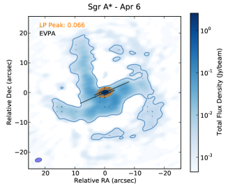
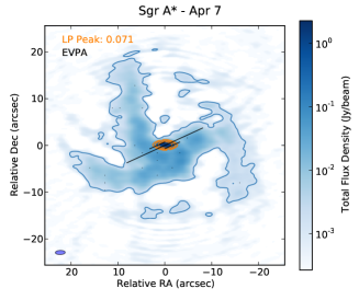
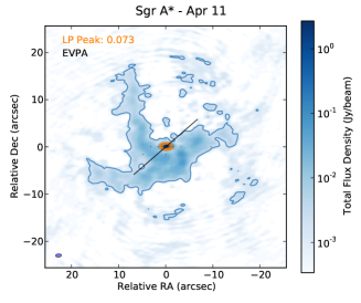
Figure 8: Polarization images of Sgr A* at 1.3 mm (see Figure 2 for a description of the plotted quantities). The apparently lower quality of the image in the right panel is due to the fact that the observations on Apr 11 have about half the beam size, and are therefore less sensitive to the extended emission in the mini-spiral, when compared to the other two days (the beamsizes are shown as ovals in the lower left corner of each panel; see values reported in Table 7). Note that there are several tiny EVPAs plotted across the mini-spiral, apparently locating regions with polarized flux above the image RMS noise cutoff ($5\sigma$). The LP and EVPA errors are however dominated by the systematic leakage (0.03% of I onto QU), which is not added to the images. Once these systematic errors are added, the LP flux in those points falls below the $3\sigma$ detection threshold. Therefore we do not claim detection of polarized emission outside of the central core in Sgr A*.

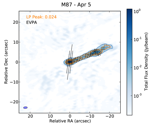
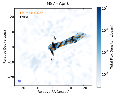
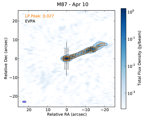
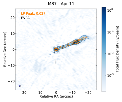
Figure 9: Polarization images of M87 at 1.3 mm (see Figure 2 for a description of the plotted quantities). The apparently different jet structures (in total and polarized intensity) across days are due to different beamsizes (shown as ovals in the lower left corner of each panel; see values reported in Table 7).

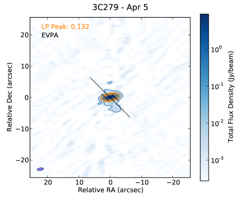
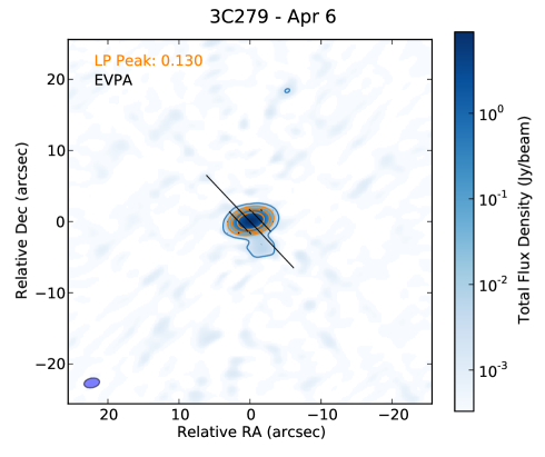
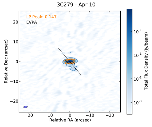
Figure 10: Polarization images of 3C279 at 1.3 mm (see Figure 2 for a description of the plotted quantities).

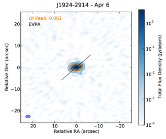
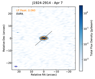
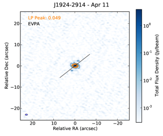
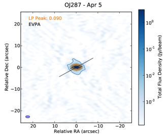
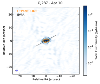
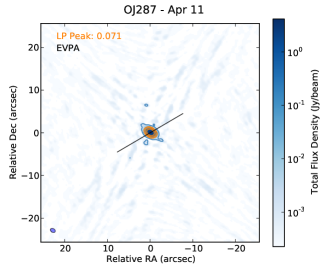
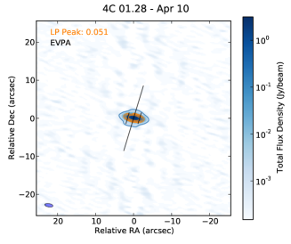
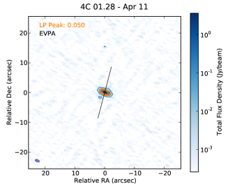
Figure 11: Polarization images of selected AGNs at 1.3 mm (see Figure 2 for a description of the plotted quantities).

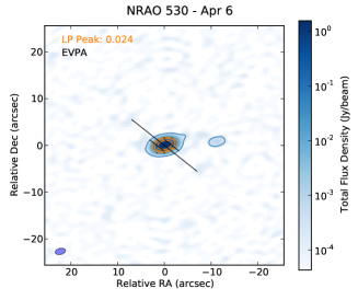
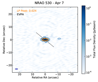
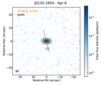
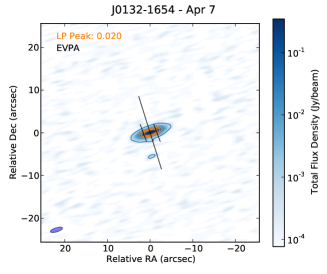
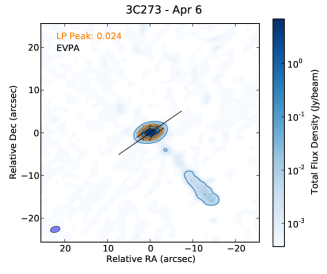
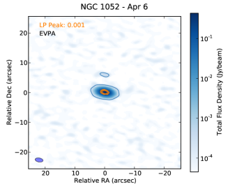
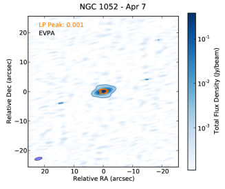
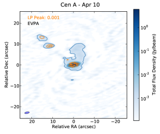
Figure 12: Polarization images of selected AGNs at 1.3 mm (see Figure 2 for a description of the plotted quantities). Note that for NGC 1052 and Cen A no EVPA could be reliably derived owing to their low level of LP. We also note that although we detect polarized flux in Cen A above the image RMS noise cutoff ($5\sigma$), once the systematic leakage (0.03% of I onto QU) is added to thermal noise, the LP flux would fall below the $3\sigma$ detection threshold. Therefore we do not claim detection of polarized emission in Cen A.

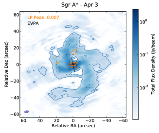
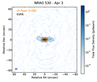
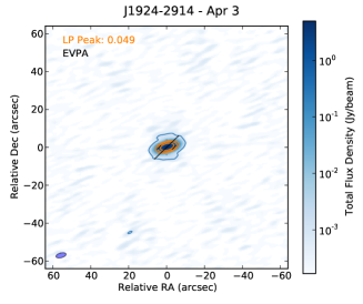
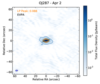
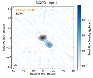
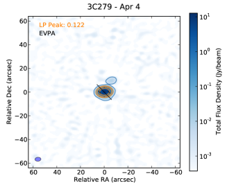
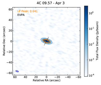
Figure 13: Polarization images of all targets observed at 3 mm (at a central frequency of 93 GHz). The beamsizes are shown as an oval in the lower left corner of each panel (see values reported in table 6). See Figure 2 for a description of the plotted quantities.

Appendix C Comparative analysis across multiple flux-extraction methods

Some of our targets (chiefly Sgr A* and M87, but also a few other AGNs; see Appendix B) reveal extended emission at arc-seconds scales, which is differently resolved out by the different observing array configurations. Here we assess the impact of such extended emission in the flux values extracted in the visibility domain for the compact cores. For this purpose, we compare the parameters derived with uvmultifit with those derived with two imaged-based methods: the sum of the nine central pixels in the clean model image (3x3) and the integrated flux (intf) from Gaussian fitting with the casa task IMFIT (see §3.2). Table 8 reports the results from this comparative analysis between the image-based and the $uv$-based methods, showing the ratio of the four Stokes parameters, the LP, and the RM (3x3/uvmf and intf/uvmf, respectively), and the difference of the EVPA in degrees (3x3-uvmf and intf-uvmf, respectively). Three sources (Cen A, NGC 1052, and J0132-1654) are excluded from this statistics due to their weak polarized signal.

Overall, the analysis clearly shows that Flux(3x3) $<$ Flux(uvmf) $<$ Flux(intf) when considering the median of the results. On the one hand, one can interpret this as the 3$\times$3 method being the least affected and intf being the most affected by extended emission (with a weak dependency on the array-configuration resolution). On the other hand, the 3$\times$3 method can also be more affected by phase and amplitude calibration errors (which will remove flux from the phase-center into the sidelobes), resulting in less recovered flux. Despite this systematic deviation, the median offsets are compatible with no significant difference within the MAD values. In Stokes $I$, both the offset and MAD are $\leq 0.4$% across the methods, which is negligible when compared to the absolute uncertainty of ALMA’s flux calibration (10% in Band 6). In the case of Stokes $Q$ and $U$, and resulting LP, the systematic offset and MAD between methods can be up to 1%. With the LP measured in our sample, these differences are generally comparable (in absolute terms) to the 0.03% of Stokes $I$ leakage onto $Q$ and $U$. The EVPA shows a MAD value of $\sim 0.1\,$deg, which results in a MAD value of up to 10% in the RM (note these are comparable or better than the observed statistical uncertainties – see Tables LABEL:tab:GMVA_uvmf_spw and LABEL:tab:EHT_uvmf_spw). The poorer results for Stokes $V$ are induced by the low level of CP in the sample (although the MAD is still comfortably around 4%).

Table 8 reports a fraction of “outliers” in the distributions (those cases that are 5$\sigma$ away from the sample median). These are generally associated with the sources with the most prominent extended emission (other outliers are associated to parameters estimated at low-significance values). In order to better assess the magnitude of these outliers, in Figure 14 we show a detailed comparison between the $uv$-based and the 3x3 image-based methods for M87 (upper panels) and Sgr A* (lower panels), respectively. Analogously to Table 8, individual panels show the ratio of the four Stokes parameters, the LP, and the RM (3x3/uvmf), and the difference of the EVPA in degrees (3x3-uvmf); the results are reported per day and SPW.

In the case of M87, the two methods exhibit an excellent agreement, except for Stokes $U$. This is due to a combination of faint $U$ emission at the core and appreciable emission from knots A and B. The discrepancy in Stokes $U$ results generally in $\Delta\rm EVPA\lesssim 0.4$^∘  comparable with the uncertainties quoted in Table LABEL:tab:EHT_uvmf_spw, with one single case of $\Delta\rm EVPA\sim 0.6$^∘ (on Apr 11 SPW=1). Given the consistency in RM (within $1\sigma$), this worst-case scenario discrepancies in EVPA do not affect the results of the analysis of this paper.

In the case of Sgr A*, the discrepancies are much more pronounced in most parameters. Despite the prominence of the mini-spiral (see §3.1 and Fig. 8), Stokes $I$ values actually agree within less than 1% between the two methods. It is however noteworthy that Flux(3x3)$>$Flux(uvmf) (i.e., the opposite trend with respect to Table 8). This inverted trend is due to a flux-decrement in the visibility amplitudes at around 25–30 k$\lambda$ affecting most prominently uvmfit on Apr 11 (this can be assessed by inspecting amplitude vs. baseline-length uv-plots – not shown here – for the parallel hands on all days). Unlike Stokes $I$, Stokes $QU$ are heavily affected, up to 20–30% in the worst cases, resulting in LP differences up to 10% and EVPA offsets up to 2^∘. These large deviations in Stokes $QU$ are systematic since all four SPW appear to deviate in each day by an approximate amount. This in turn results in consistent RM values within $1\sigma$. We note that we do not observe the same systematic offset either in M87 or J1924-2914, which were also calibrated using 3C279 as the polarization-calibrator (on Apr 6 and 11), hence we discard calibration issues as being responsible for these systematics. One possible explanation is differential Stokes $I$ leakage onto $Q$ and $U$ from extended unpolarized emission (see the spurious EVPA vectors matching the spiral-arms in Fig. 8). Note also that such unpolarized emission extends farther than the inner third of the image field of view, where beam-squash (Hull et al. 2020) combined with leakage may induce significant deviations.

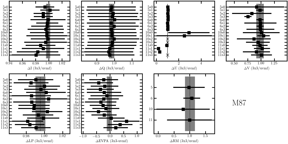
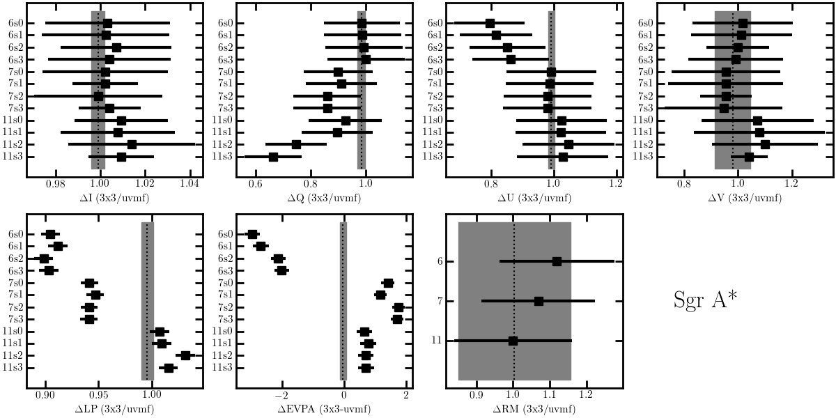
Figure 14: Comparison between image-based and $uv$-based flux-extraction methods for the two sources with the most prominent extended emission in our sample: M87 (top panels), and Sgr A* (bottom panels). The two methods being compared are: uvmultifit (uvmf) and the sum of the nine central pixels (3x3) of the model image. All parameters are compared via ratios, except for the EVPA (showing the difference in degrees). The errorbar in each data-point is the combination in quadrature of the statistical error from each flux extraction method. The vertical dotted line and the shaded region show the median and MAD from Table 8. The labels in the Y-axis indicate the observing day in April 2017 (5, 6, 7, 10, 11) and the observing SPW (s1, s2, s3, s4); the RM panel shows only the days. Non-detections in the images are indicated with a cross. Note that the plotted uncertainties are not those of individual measurements but ratios or differences between the two methods. Therefore the errors on LP and EVPA for M87 on Apr 10/11 appear comparable to other days despite the large error bars and/or non detections in Stokes $U$ (i.e. the errors in U displayed do not propagate in the LP and EVPA plots).

Given the results from this comparative analysis, we conclude that, for the purpose of the polarimetric analysis conducted in this paper, the uv-fitting method provides sufficiently accurate flux values of Stokes $IQU$ in all cases, although for Sgr A* we observe deviations in Stokes $QU$ when comparing the two flux extraction methods.

Table 8: Comparison of the three flux-extraction methods for EHT targets.

methoda	Ib	Qb	Ub	Vb	LPb	EVPAc [∘]	RMb
3x3	0.9995(0.0007)d	0.989(0.008)	0.998(0.004)	1.00(0.04)	0.993(0.006)	0.0(0.1)	1.06(0.08)
	0%d	2%	1%	5%	10%	10%	0%
intf	1.001(0.004)	1.00(0.01)	0.996(0.006)	1.00(0.04)	1.001(0.004)	0.04(0.09)	1.0(0.1)
	0%	2%	17%	10%	5%	6%	0%

Appendix D Comparison of Stokes parameters with the AMAPOLA polarimetric Grid Survey

For the purposes of absolute flux calibration, ALMA monitors the flux of bright sources (mainly blazars or QSOs) spread over the full range in right ascension (the Grid) by observing them together with solar system objects, the so-called Grid-Survey (GS), with a period of approximately 10 days. These observations are executed with the ACA, in Bands 3, 6, and 7. Since full-polarization mode is adopted, it is possible to retrieve polarimetry information from the GS sources. This is done with AMAPOLA, a set of CASA-friendly Python scripts used to reduce the full-Stokes polarimetry of GS observations with ACA. Some of our targets are part of the GS, including: 3C273 (J1229+0203); 3C279 (J1256-0547); 4C 01.28 (J1058+0133); 4C 09.57 (J1751+0939); J0510+1800; OJ287 (J0854+2006); J0006-0623; J1733-1304; and J1924-2914. Although the reported values by AMAPOLA are used for observation planning and the two arrays cover different $uv$-ranges, it is still useful to make a comparison with this database to assess any systematics or clear inconsistent variability within a week’s time-frame.

Figures 15 and 16 show the observed polarimetry parameters for the 2017 VLBI sessions (data points and errorbars), specifically $Q$, $U$, and $V$ Stokes parameters, LP, and EVPA. The shaded $\pm 1\sigma$ regions highlight the time variance of the same parameters as measured by AMAPOLA (an inflection in the trend means a time of GS observation). The colour-coding is such that blue refers to Band 3 measurements, green to Band 6, and red to Band 7 ones. These figures show that most Band 3 ALMA-VLBI measurements fall within the blue regions, while most Band 6 measurements fall in-between the blue and red regions, indicating that our measurements are broadly consistent with the AMAPOLA trends. Some potential conflicts can still be consistent with the inter-GS-cadence variability or differential time-variability between frequency bands (as also observed in some cases in the AMAPOLA monitoring). We conclude that, despite the different array specifications and data-reduction schemes, the ALMA-VLBI and AMAPOLA results are consistent between each other.

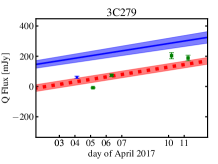
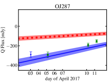
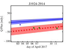
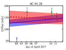
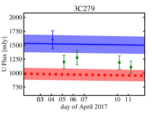
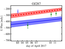
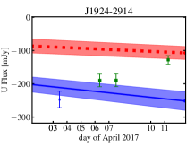
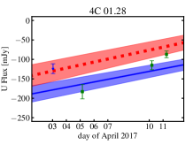
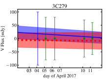
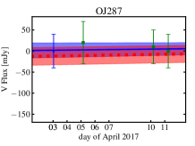
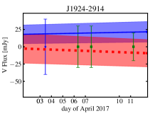
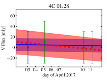
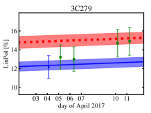
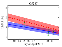
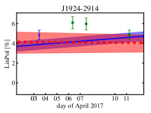
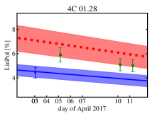
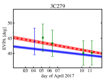
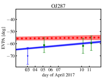
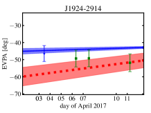
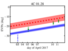
Figure 15: Comparison with time between the polarimetric results obtained for all the sources observed in the ALMA-VLBI campaign and those retrieved from the AMAPOLA polarimetric analysis of Grid Survey data. Each row shows a parameter (from top to bottom: Stokes Q, U, and V, LP, and EVPA) while each column corresponds to a source (from left to right: 3C279, OJ287, J1924-2914, and 4C 01.28; see Figure 16 for more). Only sources with entries in the ALMA archive (close in time to the observations, i.e., between end of March and April 2017) are displayed. The measured flux values during the ALMA-VLBI observations are indicated as data points and corresponding errorbars (blue and green for Band 3 and 6 observations, respectively). The shaded regions indicate AMAPOLA’s $\pm 1\sigma$ uncertainty in Band 3 (97.5 GHz; blue shade) and Band 7 (343.4 GHz; red shade), respectively. These are obtained from the ACA GS and their time evolution (lines) are obtained by interpolating between these measurements.

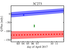
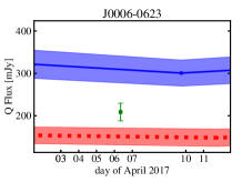
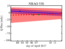
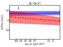
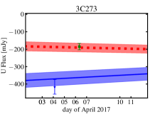
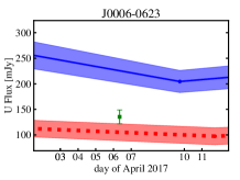
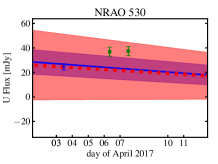
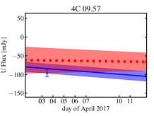
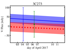
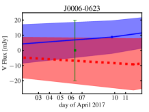
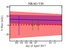
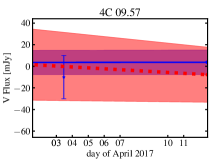
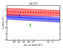
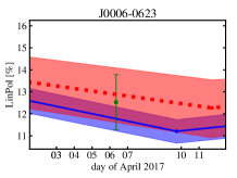
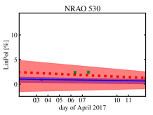
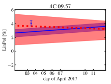
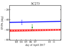
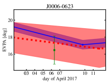
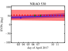
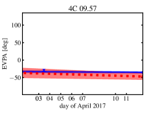
Figure 16: Same as Fig. 15, but for different sources (from left to right: 3C273, J0006-0623, NRAO 530, 4C 09.57). We note that source J0006-0623 was observed on Apr 7 but the calibrated data were of poor quality and were flagged before analysis (see § 2.2).

Appendix E Stokes parameters per ALMA frequency band (SPW)

We report the polarimetric quantities (Stokes $IQU$, LP, EVPA) per SPW in Tables LABEL:tab:GMVA_uvmf_spw (GMVA sources) and LABEL:tab:EHT_uvmf_spw (EHT sources). The Stokes parameters were fitted directly on the visibilities using uvmultifit  (see §3.2). Uncertainties are assessed with MC simulations, as the standard deviation of 1000 MC simulations for each Stokes parameter. The quoted uncertainties include in quadrature the fitting error and the Stokes $I$ leakage onto Stokes $QU$ (0.03% of $I$), as recommended by the ALMA observatory. The LP uncertainty is dominated by such systematic error, except for the weakest sources J0132-1654 and NGC 1052, for which the thermal noise starts to dominate.

In order to correct for the LP bias in the low SNR regime, we estimate a debiased LP as $\sqrt{LP^{2}-\sigma_{LP^{2}}}$, where $LP=\sqrt{Q^{2}+U^{2}}/I$.
$\sigma_{LP}$ can be estimated using propagation of errors:

$$\sigma_{LP}^{2}I^{2}= {\frac{(Q\sigma_{Q})^{2}+(U\sigma_{U})^{2}+2QU\sigma_{QU}}{Q^{2}+U^{2}}}+$$

$$[(\frac{Q}{I})^{2}+(\frac{U}{I})^{2}]\sigma^{2}_{I}-2\frac{Q}{I}\sigma_{QI}-2\frac{U}{I}\sigma_{UI}$$

where $\sigma_{I}$, $\sigma_{Q}$, $\sigma_{U}$ are the uncertainties in $I$, $Q$ and $U$, respectively. Assuming $\sigma_{QU}\sim\sigma_{QI}\sim\sigma_{UI}\sim 0$, then

$$\sigma_{LP}=\frac{1}{I}\sqrt{{\frac{(Q\sigma_{Q})^{2}+(U\sigma_{U})^{2}}{Q^{2}+U^{2}}}+[(\frac{Q}{I})^{2}+(\frac{U}{I})^{2}]\sigma^{2}_{I}}.$$

The LP values quoted in Tables 1, 2, LABEL:tab:GMVA_uvmf_spw, and LABEL:tab:EHT_uvmf_spw have this debiased correction applied. The latter does not affect most of the sources studied here, but it is especially important for the low-polarization sources such as NGC 1052 and Cen A.

The absolute flux-scale calibration systematic error (5% and 10% of Stokes $IQU$ fluxes in Band 3 and Band 6, respectively), is not included in Tables LABEL:tab:GMVA_uvmf_spw and LABEL:tab:EHT_uvmf_spw. The analysis on Stokes $V$ is performed separately (see Appendix G and Tables LABEL:tab:GMVA_uvmf_CP, LABEL:tab:EHT_uvmf_CP).

Table 9: Polarization parameters of GMVA sources per frequency band (spw) and per day.

Frequency	I	Q	U	LP	EVPA
[GHz]	[mJy]	[mJy]	[mJy]	[%]	[deg]
Apr 2
OJ287
86.3	6242.41$\pm$0.26	-409.6$\pm$1.9	-351.2$\pm$1.9	8.643$\pm$0.030	-69.69$\pm$0.10
88.3	6170.33$\pm$0.26	-410.2$\pm$1.9	-347.5$\pm$1.9	8.711$\pm$0.030	-69.87$\pm$0.10
98.3	5787.47$\pm$0.28	-398.9$\pm$1.7	-327.8$\pm$1.7	8.919$\pm$0.030	-70.30$\pm$0.10
100.3	5674.69$\pm$0.27	-392.4$\pm$1.7	-324.2$\pm$1.7	8.970$\pm$0.030	-70.214$\pm$0.093
J0510+1800
86.3	3259.30$\pm$0.57	-127.5$\pm$1.0	22.6$\pm$1.0	3.976$\pm$0.030	84.97$\pm$0.21
88.3	3208.82$\pm$0.59	-126.2$\pm$1.0	31.9$\pm$1.0	4.054$\pm$0.030	82.91$\pm$0.20
98.3	2996.03$\pm$0.62	-120.30$\pm$0.90	46.96$\pm$0.91	4.311$\pm$0.030	79.33$\pm$0.20
100.3	2962.36$\pm$0.63	-121.52$\pm$0.90	43.17$\pm$0.90	4.353$\pm$0.030	80.22$\pm$0.21
4C 01.28
86.3	5039.680$\pm$0.072	90.9$\pm$1.5	-195.6$\pm$1.5	4.281$\pm$0.030	-32.54$\pm$0.20
88.3	4970.067$\pm$0.055	93.2$\pm$1.5	-192.6$\pm$1.5	4.306$\pm$0.030	-32.09$\pm$0.20
98.3	4745.126$\pm$0.053	92.5$\pm$1.4	-194.1$\pm$1.4	4.533$\pm$0.030	-32.26$\pm$0.20
100.3	4665.997$\pm$0.054	92.1$\pm$1.4	-192.1$\pm$1.4	4.566$\pm$0.030	-32.18$\pm$0.18
Apr 3
Sgr A*
86.3	2574.84$\pm$0.87	9.28$\pm$0.77	-3.64$\pm$0.77	0.388$\pm$0.030	-10.7$\pm$2.2
88.3	2480.44$\pm$0.82	12.51$\pm$0.74	-2.36$\pm$0.74	0.513$\pm$0.030	-5.3$\pm$1.7
98.3	2514.64$\pm$0.74	18.44$\pm$0.75	16.77$\pm$0.75	0.991$\pm$0.030	21.10$\pm$0.86
100.3	2504.04$\pm$0.72	15.20$\pm$0.75	21.41$\pm$0.75	1.048$\pm$0.030	27.31$\pm$0.81
J1924-2914
86.3	5273.93$\pm$0.18	-10.6$\pm$1.6	-245.0$\pm$1.6	4.650$\pm$0.030	-46.25$\pm$0.19
88.3	5244.90$\pm$0.18	-12.7$\pm$1.6	-248.9$\pm$1.6	4.752$\pm$0.030	-46.46$\pm$0.18
98.3	4984.67$\pm$0.19	-12.0$\pm$1.5	-248.2$\pm$1.5	4.986$\pm$0.030	-46.39$\pm$0.17
100.3	4920.17$\pm$0.21	-12.3$\pm$1.5	-244.6$\pm$1.5	4.978$\pm$0.030	-46.44$\pm$0.18
NRAO 530
86.3	2857.621$\pm$0.036	7.11$\pm$0.86	24.37$\pm$0.86	0.889$\pm$0.030	36.8$\pm$1.0
88.3	2826.545$\pm$0.035	6.60$\pm$0.85	24.53$\pm$0.85	0.899$\pm$0.030	37.4$\pm$1.0
98.3	2649.116$\pm$0.034	4.24$\pm$0.80	24.59$\pm$0.80	0.943$\pm$0.030	40.08$\pm$0.92
100.3	2618.629$\pm$0.035	3.71$\pm$0.79	24.62$\pm$0.79	0.952$\pm$0.030	40.73$\pm$0.92
4C 09.57
86.3	2920.272$\pm$0.085	65.23$\pm$0.88	-98.94$\pm$0.88	4.057$\pm$0.030	-28.30$\pm$0.21
88.3	2898.304$\pm$0.073	65.59$\pm$0.87	-96.53$\pm$0.88	4.028$\pm$0.030	-27.91$\pm$0.22
98.3	2805.452$\pm$0.071	61.49$\pm$0.84	-96.65$\pm$0.85	4.084$\pm$0.030	-28.76$\pm$0.21
100.3	2775.60$\pm$0.48	60.67$\pm$0.84	-96.55$\pm$0.84	4.107$\pm$0.030	-28.93$\pm$0.22
Apr 4
3C279
86.3	13309.65$\pm$0.19	70.9$\pm$4.0	1612.7$\pm$4.0	12.129$\pm$0.030	43.746$\pm$0.071
88.3	13168.27$\pm$0.19	67.6$\pm$4.0	1596.6$\pm$4.0	12.136$\pm$0.030	43.791$\pm$0.069
98.3	12671.78$\pm$0.19	52.6$\pm$3.8	1541.8$\pm$3.8	12.175$\pm$0.030	44.021$\pm$0.070
100.3	12575.88$\pm$0.19	49.9$\pm$3.8	1533.0$\pm$3.8	12.198$\pm$0.030	44.067$\pm$0.069
3C273
86.3	10066.53$\pm$0.38	-13.8$\pm$3.0	-419.4$\pm$3.0	4.167$\pm$0.030	-45.95$\pm$0.20
88.3	10013.63$\pm$0.36	-12.3$\pm$3.0	-405.9$\pm$3.0	4.054$\pm$0.030	-45.87$\pm$0.21
98.3	9698.37$\pm$0.31	-3.3$\pm$2.9	-370.9$\pm$2.9	3.826$\pm$0.030	-45.25$\pm$0.23
100.3	9645.14$\pm$0.31	3.4$\pm$2.9	-375.2$\pm$2.9	3.891$\pm$0.030	-44.74$\pm$0.23

Table 10: Polarization parameters of EHT sources per frequency band (spw) and per day.

Frequency	I	Q	U	LP	EVPA
[GHz]	[mJy]	[mJy]	[mJy]	[%]	[deg]
Apr 5
4C 01.28
213.1	3572.28$\pm$0.11	144.5$\pm$1.1	-151.7$\pm$1.1	5.867$\pm$0.030	-23.20$\pm$0.14
215.1	3617.41$\pm$0.11	145.8$\pm$1.1	-153.3$\pm$1.1	5.848$\pm$0.030	-23.23$\pm$0.15
227.1	3429.88$\pm$0.11	138.9$\pm$1.0	-146.7$\pm$1.0	5.890$\pm$0.030	-23.28$\pm$0.14
229.1	3419.77$\pm$0.11	141.9$\pm$1.0	-147.0$\pm$1.0	5.976$\pm$0.030	-23.01$\pm$0.14
OJ287
213.1	4455.60$\pm$0.15	-214.2$\pm$1.3	-342.2$\pm$1.3	9.060$\pm$0.030	-61.027$\pm$0.092
215.1	4476.37$\pm$0.17	-214.8$\pm$1.3	-339.6$\pm$1.3	8.976$\pm$0.030	-61.161$\pm$0.092
227.1	4220.58$\pm$0.15	-205.0$\pm$1.3	-314.9$\pm$1.3	8.902$\pm$0.030	-61.53$\pm$0.10
229.1	4198.43$\pm$0.15	-203.6$\pm$1.3	-325.3$\pm$1.3	9.139$\pm$0.030	-61.022$\pm$0.093
M87
213.1	1336.29$\pm$0.13	30.07$\pm$0.40	-7.70$\pm$0.40	2.323$\pm$0.030	-7.17$\pm$0.36
215.1	1325.68$\pm$0.13	29.94$\pm$0.40	-8.10$\pm$0.40	2.338$\pm$0.030	-7.57$\pm$0.38
227.1	1236.46$\pm$0.11	29.62$\pm$0.37	-8.80$\pm$0.37	2.500$\pm$0.030	-8.29$\pm$0.35
229.1	1227.58$\pm$0.11	29.81$\pm$0.37	-8.74$\pm$0.37	2.530$\pm$0.030	-8.15$\pm$0.35
3C279
213.1	9202.50$\pm$0.11	-8.0$\pm$2.8	1214.2$\pm$2.8	13.195$\pm$0.030	45.187$\pm$0.066
215.1	9144.74$\pm$0.11	-7.2$\pm$2.7	1206.7$\pm$2.7	13.195$\pm$0.030	45.168$\pm$0.065
227.1	8845.31$\pm$0.12	-7.9$\pm$2.7	1169.0$\pm$2.7	13.216$\pm$0.030	45.193$\pm$0.063
229.1	8774.06$\pm$0.12	-6.9$\pm$2.6	1161.8$\pm$2.6	13.241$\pm$0.030	45.172$\pm$0.066
Apr 6
Sgr A*
213.1	2631.24$\pm$0.32	-130.65$\pm$0.79	-113.68$\pm$0.79	6.581$\pm$0.030	-69.49$\pm$0.13
215.1	2629.81$\pm$0.33	-128.22$\pm$0.79	-118.33$\pm$0.80	6.636$\pm$0.030	-68.65$\pm$0.13
227.1	2533.72$\pm$0.27*	-105.98$\pm$0.76	-144.59$\pm$0.76	7.076$\pm$0.030	-63.12$\pm$0.13
229.1	2625.81$\pm$0.28	-106.00$\pm$0.79	-156.22$\pm$0.79	7.188$\pm$0.030	-62.07$\pm$0.13
J1924-2914
213.1	3342.261$\pm$0.089	-28.0$\pm$1.0	-202.0$\pm$1.0	6.101$\pm$0.030	-48.95$\pm$0.14
215.1	3313.239$\pm$0.093	-28.5$\pm$1.0	-199.2$\pm$1.0	6.072$\pm$0.030	-49.07$\pm$0.14
227.1	3179.165$\pm$0.088	-30.5$\pm$1.0	-190.4$\pm$1.0	6.064$\pm$0.030	-49.55$\pm$0.14
229.1	3156.545$\pm$0.087	-30.65$\pm$0.95	-191.3$\pm$1.0	6.138$\pm$0.030	-49.55$\pm$0.14
J0132-1654
213.1	426.29$\pm$0.15	7.28$\pm$0.19	4.11$\pm$0.19	1.963$\pm$0.044	14.68$\pm$0.64
215.1	420.00$\pm$0.16	7.19$\pm$0.20	4.32$\pm$0.20	1.999$\pm$0.047	15.48$\pm$0.65
227.1	409.56$\pm$0.16	7.16$\pm$0.20	4.59$\pm$0.20	2.076$\pm$0.049	16.34$\pm$0.66
229.1	404.98$\pm$0.16	6.62$\pm$0.19	4.05$\pm$0.19	1.919$\pm$0.048	15.68$\pm$0.74
NGC 1052
213.1	437.43$\pm$0.13	0.36$\pm$0.14	0.17$\pm$0.14	0.090$\pm$0.033	13$\pm$11
215.1	438.85$\pm$0.11	0.56$\pm$0.15	0.39$\pm$0.15	0.154$\pm$0.033	17.0$\pm$6.0
227.1	414.12$\pm$0.10	0.47$\pm$0.14	0.46$\pm$0.14	0.159$\pm$0.033	21.9$\pm$6.3
229.1	415.236$\pm$0.062	0.05$\pm$0.14	0.30$\pm$0.14	0.074$\pm$0.033	39$\pm$18
M87
213.1	1361.85$\pm$0.16	27.72$\pm$0.41	-6.24$\pm$0.41	2.088$\pm$0.030	-6.34$\pm$0.43
215.1	1349.84$\pm$0.15	27.65$\pm$0.41	-6.70$\pm$0.41	2.108$\pm$0.030	-6.83$\pm$0.41
227.1	1269.57$\pm$0.13	26.95$\pm$0.38	-8.34$\pm$0.38	2.224$\pm$0.030	-8.61$\pm$0.38
229.1	1257.40$\pm$0.13	26.70$\pm$0.38	-8.28$\pm$0.38	2.224$\pm$0.030	-8.61$\pm$0.39
J0006-0623
213.1	2044.52$\pm$0.32	213.57$\pm$0.63	139.74$\pm$0.65	12.482$\pm$0.031	16.598$\pm$0.071
215.1	2023.69$\pm$0.33	212.00$\pm$0.63	137.19$\pm$0.64	12.480$\pm$0.031	16.452$\pm$0.072
227.1	1944.0$\pm$1.1	205.43$\pm$0.62	130.51$\pm$0.62	12.520$\pm$0.033	16.215$\pm$0.073
229.1	1931.6$\pm$1.1	204.15$\pm$0.61	134.03$\pm$0.62	12.645$\pm$0.033	16.646$\pm$0.074
3C279
213.1	9571.40$\pm$0.12	72.2$\pm$2.9	1240.7$\pm$2.9	12.984$\pm$0.030	43.337$\pm$0.068
215.1	9517.18$\pm$0.13	72.4$\pm$2.9	1234.1$\pm$2.9	12.990$\pm$0.030	43.324$\pm$0.067
227.1	9180.18$\pm$0.12	69.2$\pm$2.8	1193.4$\pm$2.8	13.022$\pm$0.030	43.345$\pm$0.066
229.1	9168.61$\pm$0.11	69.3$\pm$2.8	1193.1$\pm$2.8	13.035$\pm$0.030	43.338$\pm$0.066
NRAO 530
213.1	1655.066$\pm$0.071	-8.41$\pm$0.50	36.58$\pm$0.50	2.267$\pm$0.030	51.46$\pm$0.38
215.1	1669.741$\pm$0.079	-8.95$\pm$0.51	37.51$\pm$0.51	2.309$\pm$0.030	51.70$\pm$0.38
227.1	1567.831$\pm$0.072	-8.86$\pm$0.48	36.81$\pm$0.48	2.414$\pm$0.030	51.76$\pm$0.37
229.1	1554.353$\pm$0.070	-8.41$\pm$0.47	36.72$\pm$0.47	2.424$\pm$0.030	51.44$\pm$0.36
3C273
213.1	7744.46$\pm$0.11	-58.5$\pm$2.3	-191.7$\pm$2.3	2.587$\pm$0.030	-53.49$\pm$0.33
215.1	7707.72$\pm$0.11	-61.7$\pm$2.3	-186.8$\pm$2.3	2.553$\pm$0.030	-54.15$\pm$0.34
227.1	7421.16$\pm$0.10	-68.4$\pm$2.2	-153.4$\pm$2.2	2.262$\pm$0.030	-57.01$\pm$0.38
229.1	7357.33$\pm$0.10	-66.8$\pm$2.2	-145.2$\pm$2.2	2.170$\pm$0.030	-57.36$\pm$0.39
Apr 7
J1924-2914
213.1	3243.110$\pm$0.083	-26.8$\pm$1.0	-191.3$\pm$1.0	5.957$\pm$0.030	-48.99$\pm$0.15
215.1	3219.06$\pm$0.10	-27.3$\pm$1.0	-190.0$\pm$1.0	5.963$\pm$0.030	-49.09$\pm$0.15
227.1	3073.91$\pm$0.11	-27.90$\pm$0.92	-181.62$\pm$0.93	5.978$\pm$0.030	-49.37$\pm$0.14
229.1	3048.69$\pm$0.12	-28.11$\pm$0.92	-180.17$\pm$0.92	5.982$\pm$0.030	-49.44$\pm$0.15
J0132-1654
213.1	418.13$\pm$0.18	6.66$\pm$0.21	5.00$\pm$0.21	1.990$\pm$0.051	18.43$\pm$0.73
215.1	417.76$\pm$0.19	6.99$\pm$0.23	4.97$\pm$0.23	2.055$\pm$0.055	17.75$\pm$0.75
227.1	402.18$\pm$0.20	6.82$\pm$0.22	4.37$\pm$0.23	2.014$\pm$0.056	16.29$\pm$0.80
229.1	394.71$\pm$0.21	6.12$\pm$0.23	4.77$\pm$0.23	1.965$\pm$0.058	18.93$\pm$0.84
NRAO 530
213.1	1620.07$\pm$0.10	-7.36$\pm$0.49	37.57$\pm$0.49	2.363$\pm$0.030	50.55$\pm$0.35
215.1	1604.64$\pm$0.11	-7.57$\pm$0.49	37.41$\pm$0.49	2.379$\pm$0.030	50.72$\pm$0.36
227.1	1536.162$\pm$0.068	-7.65$\pm$0.47	36.73$\pm$0.47	2.443$\pm$0.030	50.89$\pm$0.37
229.1	1526.938$\pm$0.067	-7.37$\pm$0.46	37.77$\pm$0.46	2.520$\pm$0.030	50.51$\pm$0.35
Sgr A*
213.1	2418.25$\pm$0.25	-124.16$\pm$0.73	-113.45$\pm$0.73	6.954$\pm$0.030	-68.79$\pm$0.12
215.1	2404.74$\pm$0.27	-121.16$\pm$0.72	-117.97$\pm$0.72	7.032$\pm$0.030	-67.88$\pm$0.12
227.1	2318.41$\pm$0.22*	-100.51$\pm$0.70	-140.51$\pm$0.70	7.451$\pm$0.030	-62.79$\pm$0.11
229.1	2403.69$\pm$0.23	-100.83$\pm$0.72	-148.69$\pm$0.72	7.472$\pm$0.030	-62.07$\pm$0.11
NGC 1052
213.1	398.01$\pm$0.20	-0.31$\pm$0.14	0.87$\pm$0.14	0.231$\pm$0.035	54.9$\pm$4.5
215.1	397.25$\pm$0.18	-0.10$\pm$0.15	0.70$\pm$0.15	0.178$\pm$0.037	49.6$\pm$6.0
227.1	369.99$\pm$0.25	0.21$\pm$0.14	0.12$\pm$0.14	0.069$\pm$0.038	13$\pm$20
229.1	358.94$\pm$0.35	-0.46$\pm$0.14	0.44$\pm$0.14	0.177$\pm$0.039	68.1$\pm$7.9
Apr 10
4C 01.28
213.1	3668.38$\pm$0.16	154.6$\pm$1.1	-102.5$\pm$1.1	5.055$\pm$0.030	-16.77$\pm$0.16
215.1	3677.75$\pm$0.17	153.4$\pm$1.1	-102.8$\pm$1.1	5.020$\pm$0.030	-16.91$\pm$0.17
227.1	3514.62$\pm$0.14	147.8$\pm$1.1	-99.7$\pm$1.1	5.074$\pm$0.030	-17.00$\pm$0.18
229.1	3512.42$\pm$0.13	152.2$\pm$1.1	-99.6$\pm$1.1	5.179$\pm$0.030	-16.60$\pm$0.17
OJ287
213.1	4319.36$\pm$0.10	-167.8$\pm$1.3	-253.8$\pm$1.3	7.044$\pm$0.030	-61.73$\pm$0.12
215.1	4333.61$\pm$0.10	-166.9$\pm$1.3	-251.3$\pm$1.3	6.962$\pm$0.030	-61.79$\pm$0.12
227.1	4119.79$\pm$0.10	-158.1$\pm$1.2	-235.9$\pm$1.2	6.894$\pm$0.030	-61.91$\pm$0.12
229.1	4105.17$\pm$0.10	-162.0$\pm$1.2	-243.2$\pm$1.2	7.119$\pm$0.030	-61.83$\pm$0.12
Cen A
213.1	5710.166$\pm$0.085	1.8$\pm$1.7	0.5$\pm$1.7	0.040$\pm$0.030	6$\pm$30
215.1	5677.690$\pm$0.090	3.1$\pm$1.7	2.3$\pm$1.7	0.070$\pm$0.030	18$\pm$15
227.1	5621.837$\pm$0.094	3.2$\pm$1.7	4.7$\pm$1.7	0.101$\pm$0.030	27.9$\pm$9.1
229.1	5628.36$\pm$0.10	0.2$\pm$1.7	3.9$\pm$1.7	0.071$\pm$0.030	43$\pm$14
M87
213.1	1382.93$\pm$0.26	37.15$\pm$0.42	-0.24$\pm$0.42	2.688$\pm$0.030	-0.19$\pm$0.32
215.1	1371.95$\pm$0.25	37.12$\pm$0.42	-0.08$\pm$0.42	2.706$\pm$0.030	-0.08$\pm$0.31
227.1	1285.70$\pm$0.23	35.68$\pm$0.39	0.47$\pm$0.39	2.777$\pm$0.030	0.37$\pm$0.31
229.1	1271.90$\pm$0.23	35.24$\pm$0.39	0.05$\pm$0.39	2.770$\pm$0.030	0.03$\pm$0.31
3C279
213.1	8750.09$\pm$0.11	216.5$\pm$2.6	1264.2$\pm$2.6	14.659$\pm$0.030	40.141$\pm$0.057
215.1	8699.92$\pm$0.11	215.5$\pm$2.6	1257.5$\pm$2.6	14.665$\pm$0.030	40.137$\pm$0.058
227.1	8415.64$\pm$0.11	209.4$\pm$2.5	1220.6$\pm$2.5	14.717$\pm$0.030	40.133$\pm$0.058
229.1	8373.72$\pm$0.11	208.6$\pm$2.5	1216.4$\pm$2.5	14.739$\pm$0.030	40.135$\pm$0.061
Apr 11
Sgr A*
213.1	2388.59$\pm$0.31	-41.33$\pm$0.72	-169.55$\pm$0.72	7.307$\pm$0.030	-51.85$\pm$0.12
215.1	2383.72$\pm$0.30	-37.26$\pm$0.72	-169.35$\pm$0.72	7.275$\pm$0.030	-51.21$\pm$0.12
227.1	2266.69$\pm$0.26*	-13.97$\pm$0.68	-170.91$\pm$0.68	7.565$\pm$0.030	-47.34$\pm$0.11
229.1	2362.91$\pm$0.27	-12.14$\pm$0.71	-181.89$\pm$0.71	7.714$\pm$0.030	-46.91$\pm$0.12
4C 01.28
213.1	3643.15$\pm$0.20	158.8$\pm$1.1	-87.2$\pm$1.1	4.972$\pm$0.030	-14.38$\pm$0.18
215.1	3632.17$\pm$0.20	157.7$\pm$1.1	-88.5$\pm$1.1	4.980$\pm$0.030	-14.65$\pm$0.17
227.1	3503.45$\pm$0.21	152.0$\pm$1.1	-88.4$\pm$1.1	5.018$\pm$0.030	-15.10$\pm$0.17
229.1	3485.19$\pm$0.22	152.9$\pm$1.1	-87.0$\pm$1.1	5.047$\pm$0.030	-14.82$\pm$0.18
OJ287
213.1	4366.345$\pm$0.094	-148.7$\pm$1.3	-274.2$\pm$1.3	7.143$\pm$0.030	-59.23$\pm$0.12
215.1	4356.28$\pm$0.10	-151.4$\pm$1.3	-271.9$\pm$1.3	7.143$\pm$0.030	-59.56$\pm$0.12
227.1	4170.47$\pm$0.36	-149.1$\pm$1.3	-258.1$\pm$1.3	7.146$\pm$0.030	-60.01$\pm$0.12
229.1	4152.92$\pm$0.11	-145.7$\pm$1.2	-259.6$\pm$1.2	7.168$\pm$0.030	-59.65$\pm$0.12
J1924-2914
213.1	3299.39$\pm$0.19	-35.7$\pm$1.0	-156.7$\pm$1.0	4.870$\pm$0.030	-51.42$\pm$0.18
215.1	3289.89$\pm$0.19	-36.8$\pm$1.0	-155.1$\pm$1.0	4.845$\pm$0.030	-51.68$\pm$0.18
227.1	3155.4$\pm$1.0	-37.30$\pm$0.95	-147.9$\pm$1.0	4.834$\pm$0.030	-52.08$\pm$0.18
229.1	3146.13$\pm$0.17	-38.04$\pm$0.95	-149.99$\pm$0.95	4.918$\pm$0.030	-52.12$\pm$0.17
M87
213.1	1393.36$\pm$0.11	35.91$\pm$0.42	-1.16$\pm$0.42	2.579$\pm$0.030	-0.94$\pm$0.33
215.1	1380.69$\pm$0.11	36.33$\pm$0.42	-1.06$\pm$0.42	2.634$\pm$0.030	-0.85$\pm$0.33
227.1	1290.61$\pm$0.10	36.30$\pm$0.39	-0.68$\pm$0.39	2.813$\pm$0.030	-0.54$\pm$0.31
229.1	1278.47$\pm$0.10	36.23$\pm$0.39	-0.31$\pm$0.39	2.833$\pm$0.030	-0.25$\pm$0.30
3C279
213.1	8365.96$\pm$0.23	208.5$\pm$2.5	1223.0$\pm$2.5	14.830$\pm$0.030	40.163$\pm$0.059
215.1	8317.40$\pm$0.23	207.2$\pm$2.5	1217.3$\pm$2.5	14.846$\pm$0.030	40.168$\pm$0.058
227.1	8000.38$\pm$0.25	201.7$\pm$2.4	1180.8$\pm$2.4	14.974$\pm$0.030	40.154$\pm$0.058
229.1	7972.54$\pm$0.25	200.5$\pm$2.4	1178.2$\pm$2.4	14.991$\pm$0.030	40.171$\pm$0.058
*The flux of Sgr A* at 227 GHz (spw=2) is systematically $\sim$5% lower than at 229 GHz (spw=3),
owing to the presence of spectral absorption lines (see Appendix H.1).
Given its flat spectral index, $F_{spw=2}=F_{spw=3}$ should be assumed for Sgr A*.

Appendix F Faraday RM plots

We display the EVPA data as a function of $\lambda^{2}$ and their RM fitted models in Figures 17, 18, 19, and 20; EVPAs are measured in each of the four ALMA SPWs. Let us first focus on Figure 17, showing the Faraday RM of Sgr A* (upper panels), M87 (middle panels), and 3C 279 (lower panels). The EVPAs measured in Sgr A* reveal a remarkably precise $\lambda^{2}$ dependence both at $\lambda$3 mm (left panel) and $\lambda$1.3 mm (second to fourth panels). It is also remarkable that Sgr A* showcases a very consistent slope across all days, while in M87 the slope appears to change sign from Apr 5/6 to Apr 10/11. 3C 279 was used as polarization calibrator on Apr 5, 6, 10, and 11, and its measured RM (consistent with zero across all days) demonstrates the stability of the polarization measurements on M87 and on Sgr A* on the same days. On Apr 7, the polarization calibrator was J1924-2914, which also shows consistent RM across days (see Figure 18, upper panels). Collectively, they demonstrate the stability of the polarization measurements in Apr 2017 on Sgr A*, M87, and, by extension, on the remaining AGN observed at $\lambda$1.3 mm (displayed in Figure 18) and at $\lambda$3 mm (displayed in Figure 19).

We notice that, for some of the targets, the RM fits are almost perfectly consistent with the measured EVPAs; in particular, the plots for Sgr A*, 3C 279 (Fig. 17), 3C 273, J1924-2914 (Fig. 18), and M87 (Fig. 20), look very unlikely given the error bars. In fact, a standard $\chi^{2}$ analysis for these sources would give values close to 0 while for 4 points/2-parameter fit, we would expect $\chi^{2}\sim$2. This apparently unexpected behaviour can be explained by the fact that the EVPA uncertainties displayed in the RM plots are not just the thermal errors (which would naturally introduce scatter in the measurements) but also include a systematic error (0.03% of $I$ into $QU$ errors), which in fact dominates the total error budget (especially for the strongest sources with high Stokes $I$). We assessed that once such systematic error is removed, the EVPA data points are no longer consistent with the line to within their (thermal-noise-only) uncertainties. The fact that the thermal-only error bars are too small, but the error bars in the plots of this paper that include the systematic 0.03% Stokes $I$ leakage into the $QU$ error budget are too large, suggests that there is a real systematic error in the EVPA measurements but that it is smaller than the ALMA standard value. The fact that we are being conservative in our error estimates should ensure that we are not over-interpreting our measurements.

Finally, we notice that, for some of the targets and/or on specific days, there are $>1\sigma$ deviations between the observed EVPA and the RM fit-predicted values (e.g., OJ287, 4C 01.28, J0006-0623, J0510+1800; see selected panels in Figs. 18 and 19). This may suggest either the presence of an additional systematic error not accounted for in our error budget or that the assumption of the EVPA $\lambda^{2}$-dependence is not valid in some cases. In fact, in § 3.3.3,§ 5.1.1, and § 5.2 we discuss the possibility that some of the observed Faraday rotation may be partly internal, which would imply a more complex RM model than assumed in our analysis. Without a wider wavelength coverage, we cannot distinguish between the two cases. Therefore, we will not consider any additional systematic error in the RM analysis presented in this paper.

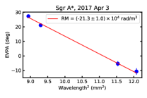
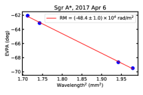
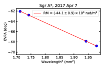
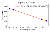
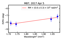
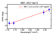
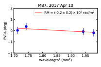
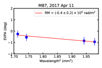
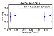
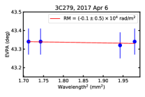
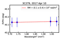
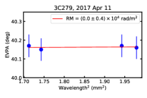
Figure 17: Faraday RM of Sgr A* (upper panels), M87 (middle panels), and 3C 279 (lower panels). The EVPA as a function of wavelength-squared is presented with $1\sigma$ error bars for each SPW and for each day. The EVPAs are measured in the 1.3 mm band, except for the upper left panel, presenting the EVPAs measured at 3 mm in Sgr A*. The error bars are derived adding in quadrature to the thermal uncertainty of the Q and U maps ($1\sigma$ image RMS) a systematic error of 0.03% of Stokes I (error bars for Sgr A* are smaller than the displayed points). The line is a linear fit to the data giving the RM reported inside the box. Plots in each row span the same vertical axis range in degrees in order to highlight differences in slope (the upper left panel is an exception). It is remarkable that Sgr A* showcases a very consistent slope across days, while in M87 the slope appears to change sign. Note also the different EVPA values between Apr 6/7 and Apr 11 in Sgr A* and between Apr 5/6 and Apr 10/11 in M87 and 3C279. The measured RM in 3C 279 (used as polarization calibrator on Apr 5, 6, 10, and 11) is consistent with zero across all days, demonstrating the stability of the polarization measurements on M87 and on Sgr A* on the same days.

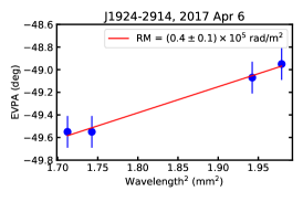
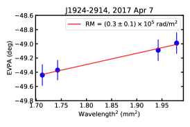
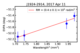
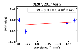
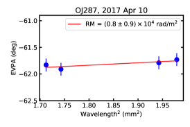
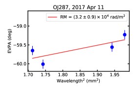
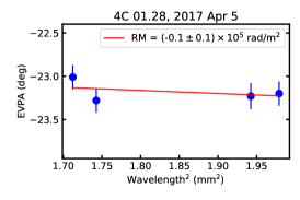
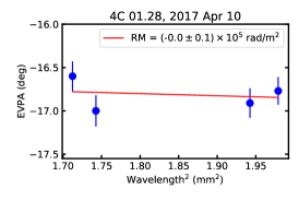
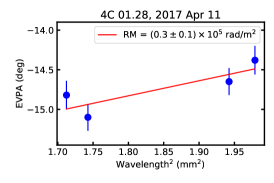
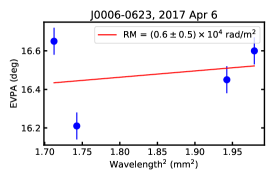
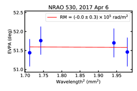
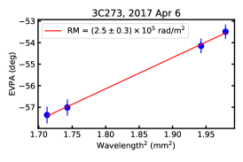
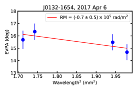
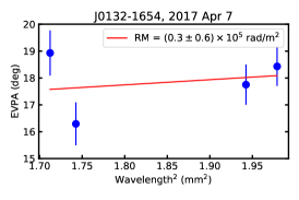
Figure 18: RM fits for remaining 2017 EHT targets with EVPA measurements at 1.3 mm (see Table 2). Plots in each row span the same vertical axis range for the same source in order to highlight differences in slope.

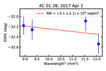
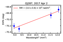
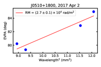
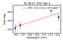
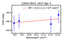
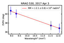
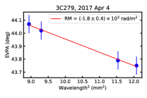
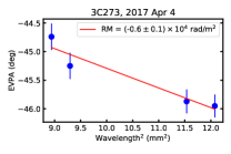
Figure 19: RM fits for the 2017 GMVA targets with EVPA measurements at 3 mm (see Table 1).

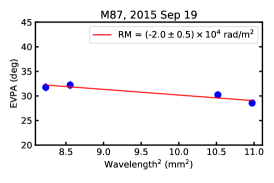
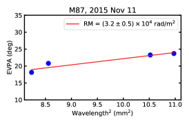
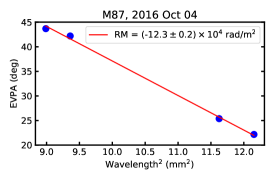
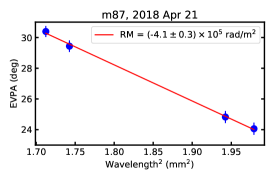
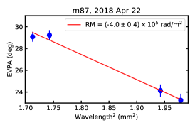
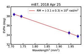
Figure 20: RM of M87 from observations carried out in Sep & Nov 2015 and Oct 2016 at 3 mm (top row) and in Apr 2018 at 1.3 mm (bottom row). Plots in both rows span the same vertical axis range (25^∘ and 8^∘ respectively) in order to highlight differences in slope (but note the different EVPA values in different panels).

Appendix G Circular Polarization and Assessment of the ALMA Polarimetry

A reliable detection of Stokes V in interferometric observations with linear-polarization feeds (i.e., the case of ALMA) strongly depends on the correct estimate of two instrumental quantities. On the one hand, the relative phase, $\Delta$, between the X and Y polarizers (i.e., the cross-polarization phase) at the reference antenna (i.e., the quantity stored in the XY0.APP table, see Goddi et al. 2019a). On the other hand, the imaginary parts of the Dterms that describe the polarization leakage of the individual ALMA elements (i.e., the quantities stored either in the Df0.APP or in the Df0.ALMA table, depending on the calibration strategy, as described in Goddi et al. 2019a). Following the standard ALMA calibration procedure, $\Delta$ is estimated by assuming a negligible Stokes V in the polarization calibrator. With this assumption, and neglecting also the effects from polarization leakage, the cross-polarization correlations ($XY^{*}$ and $YX^{*}$) between two ALMA antennas observing a polarized point source are

$$XY^{*}=e^{-j\Delta}p\sin{\left[2(\phi-\psi)\right]}~{}~{}\mathrm{and}~{}~{}YX^{*}=e^{j\Delta}p\sin{\left[2(\phi-\psi)\right]},$$ (G1)

where the data are assumed to be already corrected for phase and amplitude gains, $\psi$ and $\phi$ are the feed angle of the antennas and the EVPA of the observed source (respectively), and $p$ is the calibrator’s linearly-polarized flux density ($p=LP\times I$).

The only complex quantity that appears in Eqs. G1 is given by the factor $e^{j\Delta}$. Hence, the $XY^{*}$ (and $YX^{*}$) visibilities may change their amplitudes as a function of time (via the changes in $\psi$), but their phases will remain constant and equal to $\Delta$. The CASA-based calibration algorithm for ALMA (provided in the polcal task) takes advantage of this fact, and estimates the value of $\Delta$ from the fit of $XY^{*}$ and/or $YX^{*}$ (over different values of $\psi$) to a model with a constant phase. We call the phase estimated in this way as $\Delta_{\mathrm{QA2}}$.

G.1 Effects of an inaccurate ALMA polarization calibration

G.1.1 Polarization calibrator

If the true value of the cross-polarization phase, $\Delta$, is offset from $\Delta_{\mathrm{QA2}}$ by an unknown quantity, $\beta$ (i.e., $\Delta=\beta+\Delta_{\mathrm{QA2}}$), this offset will introduce a leakage-like effect into the polconverted VLBI visibilities, which will be described by the Dterms given in Eq. 13 of Goddi et al. (2019a). If $\beta$ is very small, that equation predicts an ALMA leakage for VLBI which has two remarkable properties: 1) it is pure imaginary, and 2) it is the same for the R and L polarization hands. The value of this Dterm is directly related to $\beta$ via the equation:

$$D^{VLBI}_{R}=D^{VLBI}_{L}\sim j\beta.$$

Therefore, if the QA2 calibration procedure has introduced an offset $\beta$ into the cross-polarization phase, $\Delta_{\mathrm{QA2}}$, we predict a pure imaginary Dterm in the ALMA-VLBI visibilities. The actual Dterms estimated from the ALMA-VLBI observations during the EHT 2017 campaign are reported in Event Horizon Telescope Collaboration et al. (2021a).

The phase offset $\beta$ may also introduce a spurious V signal into the data, which can be described by the equation (e.g., Hovatta et al. 2019)

$$V^{tot}=V^{const}\cos{\beta}+p\,\sin{\left[2\left(\phi-\psi\right)\right]}\sin{\beta},$$ (G2)

where $V^{tot}$ is the total V signal recovered from the (QA2-calibrated) data and $V^{const}$ is a constant V signal, independent of $\psi$. If the QA2 Dterm estimates for ALMA are correct, $V^{const}$ is equal to the true Stokes V of the source, (i.e., $V^{const}=V^{true}$). However, if the ALMA Dterms estimated in the QA2 are offset from their true values, there is another instrumental contribution to $XY^{*}$ and $YX^{*}$, which couples to $V^{const}$ as following

$$XY^{*} =p\,\sin{\left[2\left(\phi-\psi\right)\right]}+jV^{true}+$$ (G3)

$$\left(D_{X}^{a}+(D_{Y}^{b})^{*}\right)I+\mathcal{O}(p\,D)+\mathcal{O}(V^{true}\,D).$$

In this equation, $D_{X}^{k}$ is the part of the Dterm of the $X$ polarizer of antenna $k$ that remains uncalibrated after the QA2 (and similarly for the $Y$ polarizer). Therefore, if the effects of the antenna Dterms are not fully removed from the data, the calibrator source will show a non-negligible $V^{true}$, while the CASA model assumes it to be null.

In Fig. 21, we show the $V^{tot}$ signal (computed as the average real part of $(XY^{*}-YX^{*})/j$ among all ALMA antennas) of the polarization calibrator 3C 279, as a function of parallactic angle, for the epochs where this source was observed. We have averaged the visibilities in time bins of 120 seconds and the data taken with antenna elevations below 30 degrees have been discarded. In the figure, we also show the simple model given by Eq. G2, where $V^{const}$ and $\Delta$ are the only two free parameters used in the fit.

The V signals from the polarization calibrator show a clear dependence with parallactic angle, which indicates that there are offsets, $\beta$ in the estimated cross-polarization phases, $\Delta_{\mathrm{QA2}}$. Using the values of $p$ and $\phi$ estimated for 3C 279 on different days, we fit an X-Y phase offset of $\beta=0.2-0.5$ degrees in all tracks except April 5, where $\beta\sim 1-2$ degrees. We notice that these ranges assume no bias in the QA2 estimates of the ALMA Dterms.

It is interesting to note that the data depart from the sinusoidal model of Eq. G2, especially for the epochs on April 6 and 11, and for observations far from transit. These deviations may be related to other instrumental effects (e.g., the second-order leakage contributions, like $\mathcal{O}(p\,D)$ in Eq. G3).

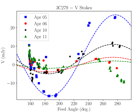
Figure 21: Reconstructed Stokes V of 3C 279 as a function of feed angle, $\phi$, during the EHT campaign. Stokes V is computed as the real part of $(XY^{*}-YX^{*})/j$. Dashed lines show the simplified model of Eq. G2, based on cross-polarization phase offset, $\beta$, of the phased-ALMA reference antenna.

From the values of $\beta$ fitted with Eq. G2, we can estimate a rough upper bound for the Stokes V of the calibrator, assuming a perfect calibration of the ALMA Dterms. For 3C 279, our analysis yields V = [27, 4, 4, 2] mJy, corresponding to CP = [0.30, 0.04, 0.07, 0.02] %, and $\beta$ = [2.2, 0.67, 0.57, 0.35] degrees, on Apr 5, 6, 10, 11, respectively. For J1924-2914, our analysis yields V = 0.7 mJy, corresponding to CP = 0.02%, and $\beta$ = -0.91 degrees, on Apr 7 (3C279 was not observed on Apr 7).

The estimated values of $V^{const}$ obtained from Eq. G2 are all of the order of 1 mJy, at most. These values are small compared to the $V^{true}$ coming from the $\beta$ estimates. This is especially true for the epoch of April 5. As discussed at the beginning of this section, a low $V^{const}$ can be explained by the compensating effect of (small) biases in the QA2 estimates of the ALMA Dterms (Eq. G3). Such systematics would force $V^{const}$ to be close to zero, regardless of the value of $V^{true}$.

In summary, two clear conclusions can be drawn from Fig. 21. On the one hand, there is an offset, $\beta$, in the X-Y cross-polarization phase of the reference antenna. On the other hand, there may be other systematics in the estimates of the antenna Dterms that may compensate the imprint of a true circular polarization of the calibrator (since CASA always assumes a null Stokes V in the calibrator).

G.1.2 Other sources

The Dterms and cross-polarization phases discussed in the previous subsection are applied to all sources in the data. Hence, the V Stokes from the polarization calibrator, which may have introduced a cross-polarization phase offset, $\beta$, and other biases to the Dterm estimates, will be systematically put back (after applying the polarization calibration) into the Stokes V signals of the rest of sources.

Thus, if we find different values of the fractional V Stokes among different sources, there has to be a contribution to their $V^{const}$ values (Eqs. G2 and G3) that is independent of that introduced by the polarization calibration. In the frame of our modelling of the instrumental polarization, such a contribution would likely be related to $V^{true}$, i.e., a true circular polarization associated to the sources.

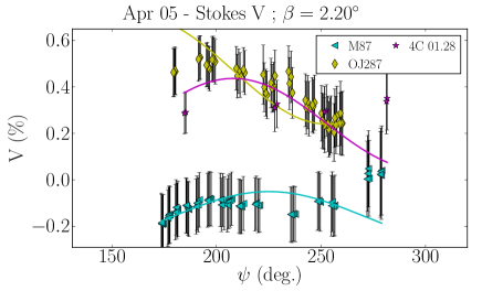
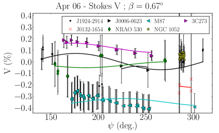
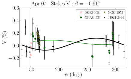
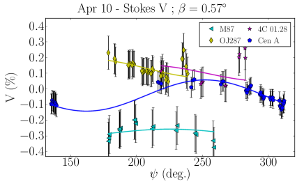
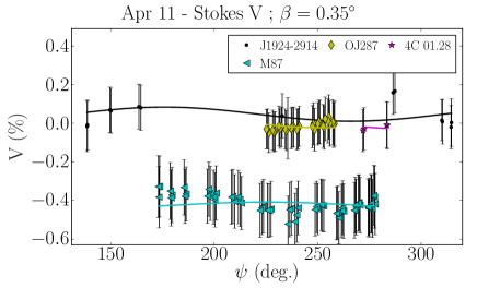
Figure 22: Reconstructed fractional Stokes V of all sources (but 3C 279), as a function of feed angle, during the EHT campaign. Stokes V is computed as the real part of $(XY^{*}-YX^{*})/j$. Continuum lines show a simplified model based on cross-polarization phase offsets at ALMA, which have been fixed to the $\beta$ values shown on top of each figure. Note that Sgr A* is not plotted because it displays significant intrinsic variability on the timescales (of hours) plotted here (e.g., Bower et al. 2018).

In Fig. 22, we show the fractional Stokes V values for all the sources, with the exception of 3C 279, as a function of feed angle. As with Fig. 21, a time binning of 120 seconds has been applied and data with elevations lower than 30 degrees have not been used. We also show the model fitted with Eq. G2, where $\beta$ is fixed to the value derived from the 3C 279 data (so the only free parameter is $V^{const}$). The only exception to this modelling is for the epoch on April 7, where J1924-291 was used instead as the polarization calibrator.

Some sources show a clear dependence of $V^{tot}$ with feed angle, being 3C 273 (on April 6) and OJ287 (on April 5) remarkable examples. However, the model prediction for such a variability, based on the cross-polarization phase offsets, $\beta$, estimated from 3C 279, cannot reproduce all the data. A possible explanation for this discrepancy could be, for instance, a small (within 1 degree) variation of $\Delta$ with pointing direction (i.e., antenna elevation and azimuth) and/or an effect related to residual Dterms (see Eq. G3). A deep analysis of these possibilities is out of the scope of this paper and should indeed be carried out at the Observatory level.

In any case, the fractional circular polarizations shown in Fig. 22 are very different among sources, which is a good indicative that these are not dominated by the Dterm systematics (at least, to a first-order approximation). Some sources do show the sinusoidal dependence with feed angle, whereas others (like M87) are dominated by $V^{const}$. Since we do not know the exact effects related to residual Dterms, it is not possible to derive $V^{true}$ from the estimated $V^{const}$. A robust conclusion, however, is that there is circular polarization detected in most of the sources (with amplitudes of the order of a few 0.1%) and that, to our understanding, the instrumental effects, alone, cannot explain the results for all sources in a self-consistent way.

Table 11: Frequency-averaged circular polarization fraction of GMVA targets (at a representative frequency of 93 GHz).

Source	Day	I	Vmeas	Vtrue	CP	LP
	[2017]	[Jy]	[mJy]	[mJy]	[%]	[%]
OJ287	Apr 2	5.97$\pm$0.30	-4$\pm$36	-3	-0.05$\pm$0.60	8.811$\pm$0.030
J0510+1800	Apr 2	3.11$\pm$0.16	-4$\pm$19	-4	-0.14$\pm$0.60	4.173$\pm$0.031
4C 01.28a	Apr 2	4.86$\pm$0.24	0$\pm$29	1.0	0.02$\pm$0.60	4.420$\pm$0.030
Sgr A*	Apr 3	2.52$\pm$0.13	-0$\pm$15	-0.5	-0.02$\pm$0.60	0.734$\pm$0.030
J1924-2914	Apr 3	5.11$\pm$0.26	0$\pm$31	5	0.09$\pm$0.60	4.841$\pm$0.031
NRAO 530a	Apr 3	2.74$\pm$0.14	0$\pm$16	0.0	0.00$\pm$0.60	0.919$\pm$0.031
4C 09.57	Apr 3	2.85$\pm$0.14	-9$\pm$17	-10	-0.34$\pm$0.60	4.069$\pm$0.030
3C279a	Apr 4	12.93$\pm$0.65	-0$\pm$78	-10	-0.1$\pm$1.2	12.159$\pm$0.030
3C273	Apr 4	9.86$\pm$0.49	11$\pm$59	14	0.14$\pm$0.60	3.984$\pm$0.029
aThe polarization calibrator is assumed to have Stokes V=0
for polarization calibration purposes (see Goddi et al. 2019a).

Table 12: Frequency-averaged circular polarization fraction of EHT targets (at a representative frequency of 221 GHz).

Source	Day	I	Vmeas	Vtrue	CP	LP
	[2017]	[Jy]	[mJy]	[mJy]	[%]	[%]
3C279a	Apr 5	8.99$\pm$0.90	0$\pm$54	27	0.30$\pm$0.60	13.210$\pm$0.030
3C279a	Apr 6	9.36$\pm$0.94	0$\pm$56	4	0.04$\pm$0.60	13.010$\pm$0.030
3C279a	Apr 10	8.56$\pm$0.86	0$\pm$51	6	0.07$\pm$0.60	14.690$\pm$0.030
3C279a	Apr 11	8.16$\pm$0.82	0$\pm$49	2	0.02$\pm$0.60	14.910$\pm$0.030
M87	Apr 5	1.28$\pm$0.13	-1.5$\pm$7.7	-2	-0.15$\pm$0.60	2.420$\pm$0.030
M87	Apr 6	1.31$\pm$0.13	-4.4$\pm$7.9	-5	-0.34$\pm$0.60	2.160$\pm$0.030
M87	Apr 10	1.33$\pm$0.13	-3.5$\pm$8.0	-4	-0.28$\pm$0.60	2.730$\pm$0.030
M87	Apr 11	1.34$\pm$0.13	-5.4$\pm$8.0	-6	-0.41$\pm$0.60	2.710$\pm$0.030
Sgr A*	Apr 6	2.63$\pm$0.26	-40$\pm$16	-40	-1.51$\pm$0.61	6.870$\pm$0.030
Sgr A*	Apr 7	2.41$\pm$0.24	-27$\pm$15	-27	-1.14$\pm$0.61	7.230$\pm$0.030
Sgr A*	Apr 11	2.38$\pm$0.24	-24$\pm$14	-24	-1.01$\pm$0.60	7.470$\pm$0.030
J1924-2914	Apr 6	3.25$\pm$0.32	0$\pm$19	0.1	0.00$\pm$0.60	6.090$\pm$0.030
J1924-2914a	Apr 7	3.15$\pm$0.31	0$\pm$19	0.7	0.02$\pm$0.60	5.970$\pm$0.030
J1924-2914	Apr 11	3.22$\pm$0.32	2$\pm$19	2	0.05$\pm$0.60	4.870$\pm$0.030
OJ287	Apr 5	4.34$\pm$0.43	17$\pm$26	20	0.46$\pm$0.60	9.020$\pm$0.030
OJ287	Apr 10	4.22$\pm$0.42	5$\pm$25	5	0.12$\pm$0.60	7.000$\pm$0.030
OJ287	Apr 11	4.26$\pm$0.43	-1$\pm$26	0.6	0.01$\pm$0.60	7.150$\pm$0.030
4C 01.28	Apr 5	3.51$\pm$0.35	10$\pm$21	9	0.25$\pm$0.60	5.890$\pm$0.030
4C 01.28	Apr 10	3.59$\pm$0.36	3$\pm$22	3	0.09$\pm$0.60	5.080$\pm$0.030
4C 01.28	Apr 11	3.57$\pm$0.36	-1$\pm$21	0.2	0.01$\pm$0.60	5.000$\pm$0.030
NRAO 530	Apr 6	1.61$\pm$0.16	-0$\pm$10	-0.4	-0.02$\pm$0.60	2.350$\pm$0.030
NRAO 530	Apr 7	1.57$\pm$0.16	0.5$\pm$9.4	0.8	0.05$\pm$0.60	2.430$\pm$0.030
J0132-1654	Apr 6	0.420$\pm$0.040	-0.7$\pm$2.5	-0.8	-0.19$\pm$0.60	1.990$\pm$0.050
J0132-1654	Apr 7	0.410$\pm$0.040	-0.1$\pm$2.5	-0.2	-0.04$\pm$0.60	2.000$\pm$0.050
NGC 1052	Apr 6	0.430$\pm$0.040	0.2$\pm$2.6	0.2	0.05$\pm$0.60	0.110$\pm$0.030
NGC 1052	Apr 7	0.380$\pm$0.040	0.4$\pm$2.3	0.3	0.08$\pm$0.60	0.150$\pm$0.040
Cen A	Apr 10	5.66$\pm$0.57	-2$\pm$34	-2	-0.04$\pm$0.60	0.060$\pm$0.030
3C273	Apr 6	7.56$\pm$0.76	10$\pm$45	9	0.12$\pm$0.60	2.390$\pm$0.030
J0006-0623	Apr 6	1.99$\pm$0.20	-1$\pm$12	-3	-0.16$\pm$0.60	12.530$\pm$0.030
aThe polarization calibrator is assumed to have Stokes V=0
for polarization calibration purposes (see Goddi et al. 2019a).

Appendix H Spectral Indices of total intensity

We compute the total intensity spectral index for all the sources observed in the VLBI campaign at 3 mm and 1.3 mm. For each source, the spectral index $\alpha$, defined as $I(\nu)\propto\nu^{\alpha}$, is derived ”in-band”, performing a weighted least-squares fit across the four flux-density values estimated with uvmultifit in each SPW, i.e. at frequencies of 213, 215, 227, 229 GHz in the 1.3 mm band, and 86, 88, 98, and 100 GHz in the 3 mm band, respectively. For Sgr A*, the spectral index of the compact core is around 0 both at 3 mm ($\alpha=0.01\pm 0.1$) and 1.3 mm ($\alpha=[-0.03,-0.15]\pm 0.06$). For M87, the spectral index of the compact core at 1.3 mm is negative ($\alpha$=[–1.2,–1.1]). Cycle 0 ALMA observations at 3 mm at a comparable angular resolution ($2.6^{\prime\prime}\times 1.4^{\prime\prime}$) yields a much flatter $\alpha$=[-0.2,-0.3] (Doi et al. 2013), consistent with VLA measurements at radio frequency bands (8.4–43 GHz). VLBA observations revealed a flat-spectrum ($\alpha$=0) compact core (e.g., Kravchenko et al. 2020). The steeper spectrum measured in the 1.3 mm band suggests that a spectral break must occur between 3 mm and 1.3 mm. Spectral steepening is also observed in other AGN sources in the sample, which vary in the range $\alpha$=[–0.7,–0.3] at 3 mm and $\alpha$=[–1.3,–0.6] at 1.3 mm (Cen A being the only exception, with $\alpha$=–0.2). When put together, these results indicates that the spectrum of AGN cores becomes progressively more optically thin at mm wavelengths (see § 5.1.1).

H.1 Foreground absorption at 226.91 GHz toward Sgr A*

Figure 23 shows the spectrum of Sgr A* in SPW=2 on 2017 Apr 07. The spectrum is virtually the same in the remainder days of observation in Apr 2017, suggesting that the absorption is probably associated with material that is in front of the galactic center core. Cyanide Radical (CN) and its hyperfine structure at 226.3600 GHz (N=2-1, J=3/2-3/2), 226.6595 GHz (N=2-1, J=3/2-1/2), and 226.8748 GHz (N=2-1, J=5/2-3/2) are identified as the carriers of the absorption features. The lines predict a loss of integrated emission over the 1.8 GHz bandwidth of about 2%, in reasonable agreement with the decrements seen in SPW=2 in Fig. 23.

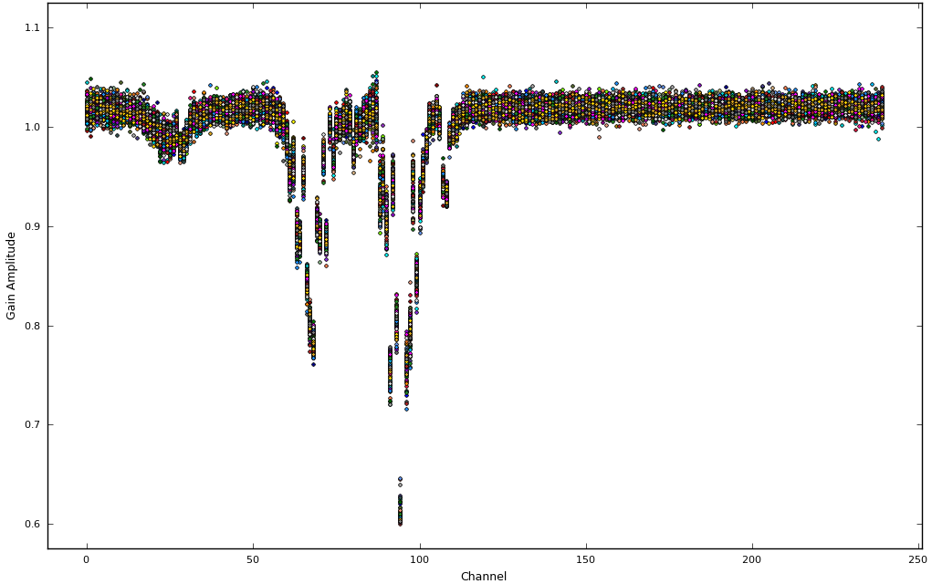
Figure 23: Bandpass for Sgr A* core (after removing instrumental bandpass with the calibrator NRAO 530) for 2017 Apr 07 observations. Only baselines longer than 60-m were used to remove virtually all of the extended arc-second emission. For each channel, every antenna bandpass amplitude is plotted (represented by different colors). All three April observations show virtually the same ‘bandpass’.

Appendix I Two-component Polarization Model for M87

Here we present the two-component polarization model for M87 summarized in Section 5.2.2 and shown schematically in Figure 6. Details of the model itself, analysis, and parameter constraints can be found below. Note that unlike the detailed image models presented in Event Horizon Telescope Collaboration et al. (2021b), these models seek to reconstruct only the Stokes $I$, $Q$, and $U$ integrated over the EHT map and within the ALMA core.

The motivation of this modeling is to assess whether or not the significant interday variations seen in the RMs of M87 can be accommodated by a model in which the only variable element is the intrinsic polarization of the horizon-scale emission, holding all other properties of the Faraday rotation and a putative large-scale polarized component fixed. In summary, we find that it is possible to do so, though it does require the RM of the horizon-scale component to be significantly larger than the RMs associated with the ALMA core in M87 reported in Table 2.

I.1 Model Definitions

We consider two two-component models for the polarimetric properties of M87, differing in the location of the small-scale Faraday screen. For both components, we construct the set of Stokes $I$, $Q$, $U$, which may depend on observation day and wavelength. The directly compared quantities that comprise the model are the integrated Stokes parameters of the compact component, $I_{\rm com,day,\lambda}$, $Q_{\rm com,day,\lambda}$, and $U_{\rm com,day,\lambda}$, and of the combination of the compact and extended components, $I_{\rm tot,day,\lambda}=I_{\rm com,day,\lambda}+I_{\rm ext,\lambda}$, $Q_{\rm tot,day,\lambda}=Q_{\rm com,day,\lambda}+Q_{\rm ext,\lambda}$, and $U_{\rm tot,day,\lambda}=U_{\rm com,day,\lambda}+U_{\rm ext,\lambda}$. A summary list of the model parameters for the models described in Sections I.1.1-I.1.3 is contained in Table 13.

I.1.1 Extended component

Both models contain a large-scale component defined by an intensity normalization $I_{0,\rm ext}$ at a reference wavelength $\lambda_{0}$, spectral index $\alpha_{0,\rm ext}$, polarization fraction $m_{\rm ext}$, and EVPA $\psi_{\rm ext}$ at $\lambda_{0}$. This is further processed through an external Faraday screen with a rotation measure of ${\rm RM}_{\rm ext}$. The contribution to the Stokes $I$, $Q$, and $U$ are, then

$$I_{{\rm ext},\lambda} =I_{0,\rm ext}\left(\lambda/\lambda_{0}\right)^{\alpha_{\rm ext}}$$ (I1)

$$Q_{{\rm ext},\lambda} =m_{\rm ext}I_{{\rm ext},\lambda}\cos\left[2\psi+2{\rm RM}_{\rm ext}(\lambda^{2}-\lambda_{0}^{2})\right]$$

$$U_{{\rm ext},\lambda} =m_{\rm ext}I_{{\rm ext},\lambda}\sin\left[2\psi+2{\rm RM}_{\rm ext}(\lambda^{2}-\lambda_{0}^{2})\right]$$

This introduces five parameters: $I_{0,\rm ext}$, $\alpha_{\rm ext}$, ${\rm RM_{\rm ext}}$, $m_{\rm ext}$, and $\psi$.

I.1.2 Compact component: external Faraday screen

For each day on which M87 was observed by ALMA and the EHT (i.e., April 5, 6, 10 and 11) we specify a similar model for the compact component. When the screen is assumed to be external, we adopt a similar model to the large-scale component with the exception that the rotation is due to both screens:

$$I^{\rm Ex}_{{\rm com},{\rm day},\lambda} =I_{0,\rm com}\left(\lambda/\lambda_{0}\right)^{\alpha_{\rm com}}$$ (I2)

$$Q^{\rm Ex}_{{\rm com},{\rm day},\lambda} =m_{\rm com,day}I^{\rm Ex}_{{\rm com},{\rm day},\lambda}$$

$$\cos\left[2\psi_{\rm com,day}+2({\rm RM_{\rm com}}+{\rm RM}_{\rm ext})(\lambda^{2}-\lambda_{0}^{2})\right]$$

$$U^{\rm Ex}_{{\rm com},{\rm day},\lambda} =m_{\rm com,day}I^{\rm Ex}_{{\rm com},{\rm day},\lambda}$$

$$\sin\left[2\psi_{\rm com,day}+2({\rm RM_{\rm com}}+{\rm RM}_{\rm ext}(\lambda^{2}-\lambda_{0}^{2})\right].$$

This introduces an additional eleven parameters: $I_{0,\rm com}$, $\alpha_{\rm com}$, ${\rm RM_{\rm com}}$, and four each $m_{\rm com,day}$ and $\psi_{\rm com,day}$. The polarization fraction and EVPA of the compact component, $m_{\rm com,day}$ and $\psi_{\rm com,day}$, are distinct from all of the other parameters in the model in that they vary among observation days. Therefore, where useful, we will distinguish these as “dynamic” parameters, with the remainder of the parameters being “static” in the limited sense that they do not vary across the observation campaign.

I.1.3 Compact component: internal Faraday screen model

Many simulations of M87 indicate the presence of large Faraday depths in the emission region (Broderick & McKinney 2010; Mościbrodzka et al. 2017; Ricarte et al. 2020). Therefore, we also consider a simple model for the compact component in which the emission and rotation are co-located, i.e., an internal Faraday screen. In principle, this is inextricably linked to the detailed properties of the emission region. Here we employ the gross simplification of a single-zone, or slab, model: the emission and Faraday rotation within the compact component occurs within a homogeneous region. We begin with a summary of the polarimetric properties of such a slab.

For a plane-parallel source with physical depth $L$ and at some reference wavelength $\lambda_{0}$ a uniform emissivity $j$, polarization fraction $m_{\rm em}$ at emission, EVPA at emission $\psi_{\rm em}$, Faraday rotativity $R$, we have total intensity,

$$I=\int_{0}^{L}jdz=jL,$$ (I3)

and Stokes $Q$ and $U$,

$$Q+iU =\int_{0}^{L}jm_{\rm em}e^{2i[Rx\lambda^{2}+\psi_{\rm em}]}dx$$ (I4)

$$=\frac{m_{\rm em}I}{2RL\lambda^{2}}\left[\sin(2\psi_{\rm em}+2RL\lambda^{2})-\sin(2\psi_{\rm em})\right]$$

$$+i\frac{m_{\rm em}I}{2RL\lambda^{2}}\left[\cos(2\psi_{\rm em})-\cos(2\psi_{\rm em}+2RL\lambda^{2})\right]$$

$$=\frac{1}{2}m_{\rm em}I{\rm sinc}(RL\lambda^{2})$$

$$\left[\cos(2\psi_{\rm em}+RL\lambda^{2})+i\sin(2\psi_{\rm em}+RL\lambda^{2})\right]$$

from which we can immediately read off $Q$ and $U$. The EVPA at the top of the slab is

$$\tan(2\psi)=\frac{Q}{U}=\tan\left[2\psi_{\rm em}+RL(\lambda^{2}-\lambda_{0}^{2})\right],$$ (I5)

from which it is apparent that the effective contribution to the compact RM is ${\rm RM}_{\rm com}=RL/2$.

The internal Faraday screen model is then defined by

$$I^{\rm In}_{{\rm com},{\rm day},\lambda} =I_{0,\rm com}\left(\lambda/\lambda_{0}\right)^{\alpha_{\rm com}}$$ (I6)

$$Q^{\rm In}_{{\rm com},{\rm day},\lambda} =\frac{1}{2}m_{\rm com,day}I^{\rm In}_{{\rm com},{\rm day},\lambda}{\rm sinc}(2{\rm RM}_{\rm com}\lambda^{2})$$

$$\cos\left[2\psi_{\rm com,day}+2({\rm RM}_{\rm com}+{\rm RM}_{\rm ext})\lambda^{2}\right]$$

$$U^{\rm In}_{{\rm com},{\rm day},\lambda} =\frac{1}{2}m_{\rm com,day}I^{\rm In}_{{\rm com},{\rm day},\lambda}{\rm sinc}(2{\rm RM}_{\rm com}\lambda^{2})$$

$$\sin\left[2\psi_{\rm com,day}+2({\rm RM}_{\rm com}+{\rm RM}_{\rm ext})\lambda^{2}\right],$$

where, as with the external model, we have added the Faraday rotation from the large-scale Faraday screen. As with the external Faraday screen model, this introduces eleven parameters, though the interpretations of the polarization fraction, and EVPA subtly differ, here referring to those of the emission process instead of derotated values.

As with the external Faraday screen model, where useful, we will refer to $m_{\rm com,day}$ and $\psi_{\rm com,day}$, which differ among observation days, as “dynamic” parameters to distinguish them from the remaining “static” parameters.

I.2 Markov Chain Monte Carlo Analysis

From the models described above and the integrated EHT Stokes parameter ranges presented in Table 7 in Appendix H2 of Event Horizon Telescope Collaboration et al. (2021a) ($I_{\rm EHT}$, $Q_{\rm EHT}$, $U_{\rm EHT}$) and the ALMA core Stokes parameter values for the individual SPWs in Table LABEL:tab:EHT_uvmf_spw ($I_{\rm spw}$, $Q_{\rm spw}$, $U_{\rm spw}$), we construct a log-likelihood for each set of model parameters. These comprise sixty data values in total: three ($I_{\rm EHT}$, $Q_{\rm EHT}$, $U_{\rm EHT}$) on each of four days from the EHT observations ($3\times 4$ data points), three ($I_{\rm spw}$, $Q_{\rm spw}$, $U_{\rm spw}$) in four SPWs on each of four days presented here ($3\times 4\times 4$ data points).

We assume that the integrated EHT Stokes parameters are distributed normally with means and standard deviations set by the centers and half-widths of the ranges; this likely over-estimates the true uncertainty on the $I_{\rm EHT}$, $Q_{\rm EHT}$, and $U_{\rm EHT}$. The resulting log-likelihood is

$$\mathcal{L}=\sum_{\rm day}\Bigg{[}-\frac{(I_{\rm EHT}-I_{\rm com,day,\lambda_{0}})^{2}}{2\sigma_{I_{\rm EHT}}^{2}}-\frac{(Q_{\rm EHT}-Q_{\rm com,day,\lambda_{0}})^{2}}{2\sigma_{Q_{\rm EHT}}^{2}}\\ -\frac{(U_{\rm EHT}-U_{\rm com,day,\lambda_{0}})^{2}}{2\sigma_{U_{\rm EHT}}^{2}}-\sum_{\rm spw=1}^{4}\frac{(I_{\rm spw}-I_{\rm tot,day,\lambda_{\rm spw}})^{2}}{2\sigma_{I_{\rm spw}}^{2}}\\ -\sum_{\rm spw=1}^{4}\frac{(Q_{\rm spw}-Q_{\rm tot,day\lambda_{\rm spw}})^{2}}{2\sigma_{Q_{\rm spw}}^{2}}-\sum_{\rm spw=1}^{4}\frac{(U_{\rm spw}-U_{\rm tot,day,\lambda_{\rm spw}})^{2}}{2\sigma_{U_{\rm spw}}^{2}}\Bigg{]}.$$ (I7)

Linear or ”uniform” priors in the natural ranges are imposed on all parameters with the exception of the compact and extended component intensity normalizations, for which logarithmic priors are chosen. See Table 13 for details.

The likelihood is sampled with the ensemble Markov Chain Monte Carlo (MCMC) method provided by the EMCEE python package (Foreman-Mackey et al. 2013). We use 256 independent walkers, and run for $10^{5}$ steps, discarding the first half of the chains. Explorations with fewer walkers and steps indicate that by this time the MCMC chains are well converged.

In addition to the models described in Appendix I.1, we also considered versions of the two-component model applied to each day independently, i.e., keeping only one day in the sum in Equation I7. In these, on each day the five parameters of the external screen and five parameters of the internal screen (a single $m_{\rm com}$ and $\psi_{com}$) are independently fit on each observation day. Effectively, this corresponds to a forty-parameter model across the four observation days, permitting Faraday screens and emission from both the compact and extended Faraday screens to vary independently across the four observation days.

On any given observation day, the parameters are less well constrained in this case and, with the notable exceptions of the compact component polarization fraction and EVPA, are consistent with a single set of values across all days. The variable polarization properties of the compact component matches the expectation from the EHT measurements in Event Horizon Telescope Collaboration et al. (2021a). The consistency with a single set of values for the remaining model parameters serves as a partial motivation for the more restricted variability in the models presented in Appendix I.1.

I.3 Two-component model results

Excellent fits are found for both the external and internal Faraday screen models. For 44 degrees of freedom, the best-fit external and internal screen models have reduced $\chi^{2}=3.96$ and $\chi^{2}=2.54$, respectively, both modestly small and possibly indicating that the uncertainties on the integrated EHT Stokes parameters are indeed over estimated by their half-range values. Thus, it is possible to reproduce the variable polarimetric properties observed by ALMA with a model in which only the compact emission evolves.

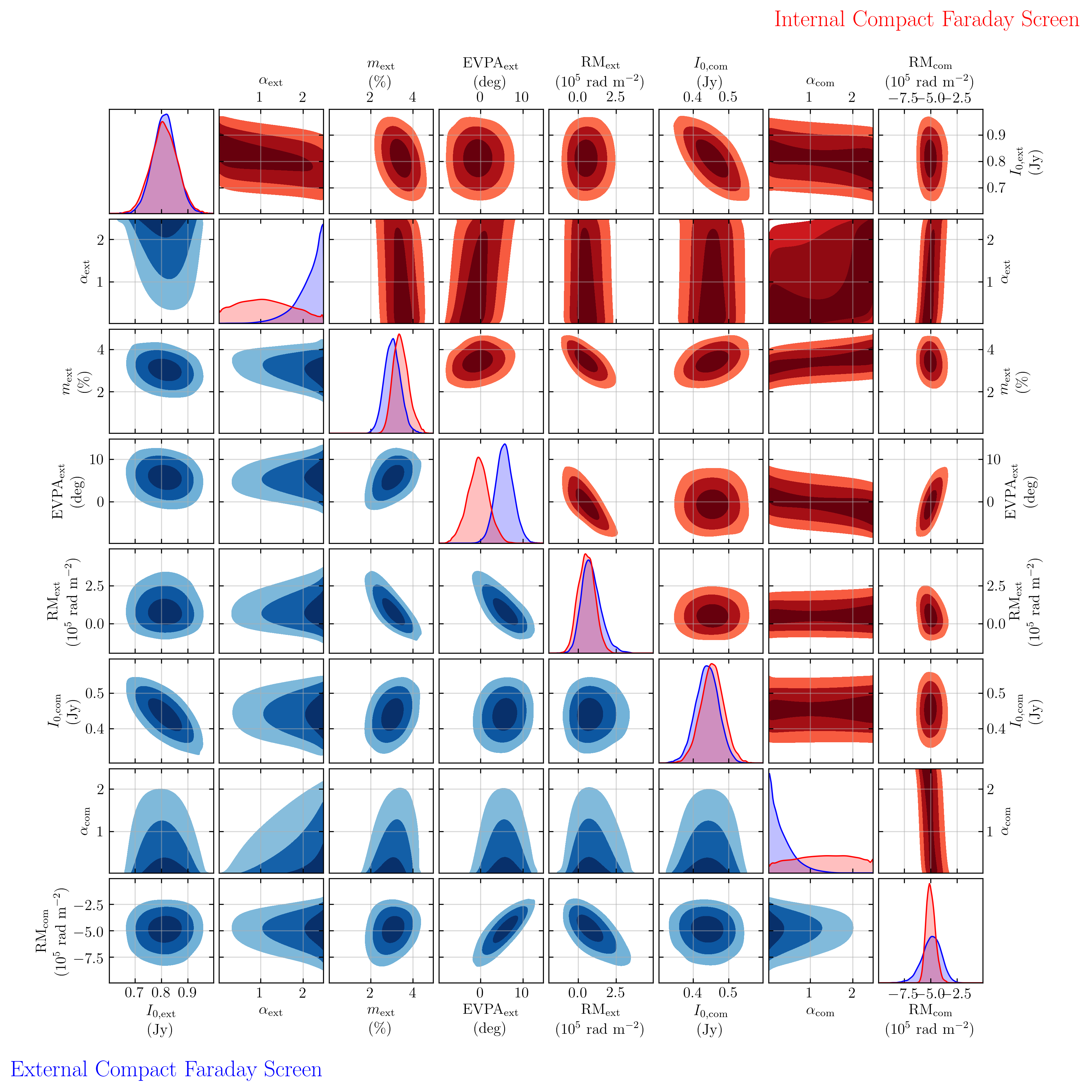
Figure 24: Joint posteriors for static parameters of two-component polarimetric models with external (lower left; blue) and internal (upper right; red) small-scale Faraday screens. Contours indicate 50%, 90%, and 95% quantiles.

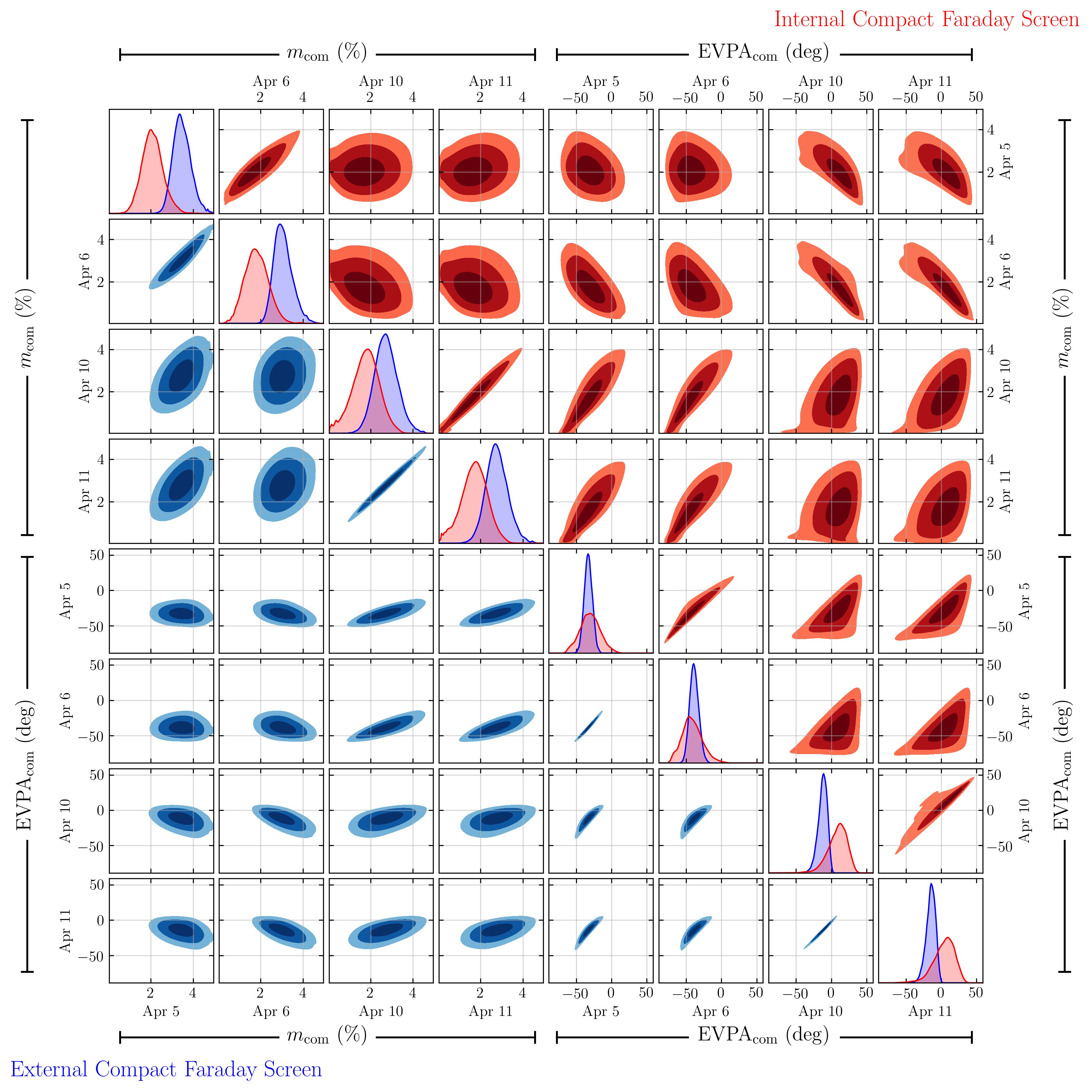
Figure 25: Joint posteriors for dynamic parameters of two-component polarimetric models with external (lower left; blue) and internal (upper right; red) small-scale Faraday screens. For the internal Faraday screen model, the polarization fractions have been depolarized by a factor of ${\rm sinc}(2{\rm RM}_{\rm com}\lambda_{0}^{2})$ and the EVPAs have been rotated by $({\rm RM}_{\rm com}+{\rm RM}_{\rm ext})\lambda_{0}^{2}$, corresponding to observed values, concordant with the definition for the external Faraday screen model. Contours indicate 50%, 90%, and 95% quantiles.

Table 13: Two-component model MCMC analysis priors and results.

Parameter	Unit	Prior	External Screen	Internal Screen
$I_{0,\rm ext}$	Jy	$\mathcal{L}(0,\infty)$	$0.813\pm 0.044$	$0.811\pm 0.049$
$\alpha_{\rm ext}$	–	$\mathcal{U}[0,2.5]$	$2.14\pm 0.32$	$1.12\pm 0.62$
$m_{\rm ext}$	%	$\mathcal{U}[0,100]$	$3.03\pm 0.37$	$3.43\pm 0.36$
${\rm EVPA}_{\rm ext}$	deg	$\mathcal{U}[-90,90]$	$5.7\pm 2.1$	$-0.5\pm 2.4$
${\rm RM}_{\rm ext}$	$10^{5}~{}{\rm rad~{}m^{-2}}$	$\mathcal{U}[-100,100]$	$0.87\pm 0.64$	$0.55\pm 0.53$
$I_{0,\rm com}$	Jy	$\mathcal{L}(0,\infty)$	$0.439\pm 0.032$	$0.454\pm 0.032$
$\alpha_{\rm com}$	–	$\mathcal{U}[0,2.5]$	$0.31\pm 0.27$	$1.31\pm 0.66$
${\rm RM}_{\rm com}$	$10^{5}~{}{\rm rad~{}m^{-2}}$	$\mathcal{U}[-100,100]$	$-4.92\pm 0.91$	$-4.98\pm 0.43$
$m_{\rm com,Apr~{}5~{}}$	%	$\mathcal{U}[0,100]$	$3.48\pm 0.41$	$3.66\pm 0.66$
$m_{\rm com,Apr~{}6~{}}$	%	$\mathcal{U}[0,100]$	$3.06\pm 0.43$	$3.17\pm 0.82$
$m_{\rm com,Apr~{}10}$	%	$\mathcal{U}[0,100]$	$2.73\pm 0.54$	$3.2\pm 1.2$
$m_{\rm com,Apr~{}11}$	%	$\mathcal{U}[0,100]$	$2.78\pm 0.51$	$3.0\pm 1.1$
${\rm EVPA}_{\rm com,Apr~{}5~{}}$	deg	$\mathcal{U}[-90,90]$	$-32.9\pm 5.6$	$14\pm 10$
${\rm EVPA}_{\rm com,Apr~{}6~{}}$	deg	$\mathcal{U}[-90,90]$	$-38.5\pm 6.3$	$3.0\pm 10.0$
${\rm EVPA}_{\rm com,Apr~{}10}$	deg	$\mathcal{U}[-90,90]$	$-12.4\pm 6.5$	$53\pm 13$
${\rm EVPA}_{\rm com,Apr~{}11}$	deg	$\mathcal{U}[-90,90]$	$-14.8\pm 6.6$	$48\pm 13$

Figures 24 and 25 show the joint posteriors for the external (lower left) and internal (upper right) Faraday screen models for the static and dynamic model components, respectively. To facilitate a direct comparison with the external Faraday screen model, in Figure 25, the polarization fractions and EVPAs of the internal Faraday screen model have been depolarized and rotated to show the corresponding posteriors on their observed analogs. Model parameter estimates, marginalized over all other parameters, are contained in Table 13.

After adjusting the polarization fraction and EVPA of the compact component, the properties of the two-component models are consistent among the external and internal Faraday screen models. Strong correlations exists between many of the compact component features. These are very strong for the polarization fractions and EVPAs on neighboring observation days, i.e., April 5 and 6, and April 10 and 11. This is anticipated by the similarities in the integrated polarimetric properties reported in Event Horizon Telescope Collaboration et al. (2021a) between neighboring observation days, which naturally constrain the two-component polarization models accordingly.

The flux normalizations, polarization fractions, and EVPAs are well constrained. ${\rm RM}_{\rm ext}$ is restricted to small magnitudes in both cases, typically less than $1.5\times 10^{5}~{}{\rm rad~{}m^{-2}}$, and remains consistent with vanishing altogether. In contrast, ${\rm RM}_{\rm com}$ is significantly non-zero, and typically of order $-5\times 10^{5}~{}{\rm rad~{}m^{-2}}$, factors of 3-10 larger than those reported in Table 2, implying a significant degree of competition between the spectral variations in the two components and the residual Faraday rotation. In neither model are the spectral indexes of the components well constrained.

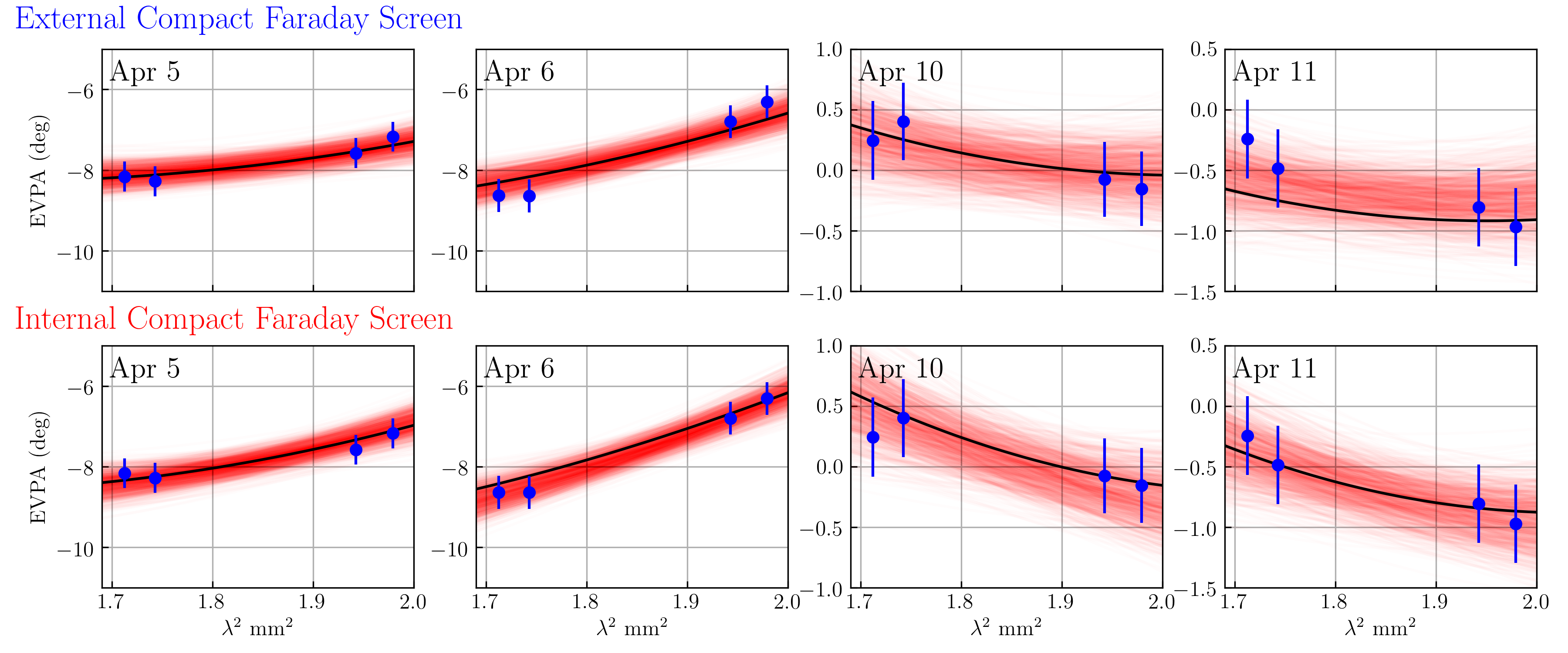
Figure 26: EVPA as a function of $\lambda^{2}$ for $10^{3}$ draws from the two-component model posterior of the external (top) and internal (bottom) Faraday screen models. The highest-likelihood models are shown by the black lines. The blue data points are the ALMA measurements (same as Fig. 17).

By construction, these are necessarily consistent with the results from ALMA-only RM measurements reported in Table 2. Figure 26 shows a number of realizations drawn from the posteriors for the wavelength-dependence of the EVPAs on each of the observation days in comparison to the measured values listed in Table LABEL:tab:EHT_uvmf_spw. The interday evolution in the ALMA RMs are well reproduced, despite restricting the variable elements of the model to the compact component. Within the ALMA SPWs the EVPAs only weakly depart from the linear dependence on $\lambda^{2}$ indicative of Faraday rotation; outside of the ALMA SPWs this divergence can become considerably larger, implying that additional coincident polarimetric measurements at longer (and shorter) wavelengths will significantly improve constraints on the elements of the two-component model.

References

- Agudo et al. (2014) Agudo, I., Thum, C., Gómez, J. L., & Wiesemeyer, H. 2014, A&A, 566, A59, doi: 10.1051/0004-6361/201423366
- Agudo et al. (2018) Agudo, I., Thum, C., Ramakrishnan, V., et al. 2018, MNRAS, 473, 1850, doi: 10.1093/mnras/stx2437
- Algaba et al. (2016) Algaba, J. C., Asada, K., & Nakamura, M. 2016, ApJ, 823, 86, doi: 10.3847/0004-637X/823/2/86
- Asada et al. (2002) Asada, K., Inoue, M., Uchida, Y., et al. 2002, PASJ, 54, L39, doi: 10.1093/pasj/54.3.L39
- Baczko et al. (2016) Baczko, A. K., Schulz, R., Kadler, M., et al. 2016, A&A, 593, A47, doi: 10.1051/0004-6361/201527951
- Beckert & Falcke (2002) Beckert, T., & Falcke, H. 2002, A&A, 388, 1106, doi: 10.1051/0004-6361:20020484
- Biretta et al. (1995) Biretta, J. A., Zhou, F., & Owen, F. N. 1995, ApJ, 447, 582, doi: 10.1086/175901
- Blandford et al. (2019) Blandford, R., Meier, D., & Readhead, A. 2019, ARA&A, 57, 467, doi: 10.1146/annurev-astro-081817-051948
- Blandford & Begelman (1999) Blandford, R. D., & Begelman, M. C. 1999, MNRAS, 303, L1, doi: 10.1046/j.1365-8711.1999.02358.x
- Blandford & Königl (1979) Blandford, R. D., & Königl, A. 1979, ApJ, 232, 34, doi: 10.1086/157262
- Blandford & Payne (1982) Blandford, R. D., & Payne, D. G. 1982, MNRAS, 199, 883, doi: 10.1093/mnras/199.4.883
- Blandford & Znajek (1977) Blandford, R. D., & Znajek, R. L. 1977, MNRAS, 179, 433, doi: 10.1093/mnras/179.3.433
- Bower et al. (2017) Bower, G. C., Dexter, J., Markoff, S., Rao, R., & Plambeck, R. L. 2017, ApJ, 843, L31, doi: 10.3847/2041-8213/aa7b2e
- Bower et al. (1999a) Bower, G. C., Falcke, H., & Backer, D. C. 1999a, ApJ, 523, L29, doi: 10.1086/312246
- Bower et al. (2002) Bower, G. C., Falcke, H., Sault, R. J., & Backer, D. C. 2002, ApJ, 571, 843, doi: 10.1086/340064
- Bower et al. (2005) Bower, G. C., Falcke, H., Wright, M. C., & Backer, D. C. 2005, ApJ, 618, L29, doi: 10.1086/427498
- Bower et al. (1999b) Bower, G. C., Wright, M. C. H., Backer, D. C., & Falcke, H. 1999b, ApJ, 527, 851, doi: 10.1086/308128
- Bower et al. (2001) Bower, G. C., Wright, M. C. H., Falcke, H., & Backer, D. C. 2001, ApJ, 555, L103, doi: 10.1086/323180
- Bower et al. (2003) —. 2003, ApJ, 588, 331, doi: 10.1086/373989
- Bower et al. (2018) Bower, G. C., Broderick, A., Dexter, J., et al. 2018, ApJ, 868, 101, doi: 10.3847/1538-4357/aae983
- Brentjens & de Bruyn (2005) Brentjens, M. A., & de Bruyn, A. G. 2005, A&A, 441, 1217, doi: 10.1051/0004-6361:20052990
- Briggs (1995) Briggs, D. S. 1995, in American Astronomical Society Meeting Abstracts, Vol. 187, American Astronomical Society Meeting Abstracts, 112.02
- Broderick & Loeb (2009) Broderick, A. E., & Loeb, A. 2009, ApJ, 697, 1164, doi: 10.1088/0004-637X/697/2/1164
- Broderick & McKinney (2010) Broderick, A. E., & McKinney, J. C. 2010, ApJ, 725, 750, doi: 10.1088/0004-637X/725/1/750
- Cioffi & Jones (1980) Cioffi, D. F., & Jones, T. W. 1980, AJ, 85, 368, doi: 10.1086/112685
- Clarke et al. (1992) Clarke, D. A., Burns, J. O., & Norman, M. L. 1992, ApJ, 395, 444, doi: 10.1086/171663
- Contopoulos & Kazanas (1998) Contopoulos, I., & Kazanas, D. 1998, Astrophys. J., 508, 859, doi: 10.1086/306426
- Davelaar et al. (2019) Davelaar, J., Olivares, H., Porth, O., et al. 2019, A&A, 632, A2, doi: 10.1051/0004-6361/201936150
- de Gasperin et al. (2012) de Gasperin, F., Orrú, E., Murgia, M., et al. 2012, A&A, 547, A56, doi: 10.1051/0004-6361/201220209
- Dexter et al. (2012) Dexter, J., McKinney, J. C., & Agol, E. 2012, MNRAS, 421, 1517, doi: 10.1111/j.1365-2966.2012.20409.x
- Di Matteo et al. (2003) Di Matteo, T., Allen, S. W., Fabian, A. C., Wilson, A. S., & Young, A. J. 2003, ApJ, 582, 133, doi: 10.1086/344504
- Doeleman et al. (2008) Doeleman, S. S., Weintroub, J., Rogers, A. E. E., et al. 2008, Nature, 455, 78, doi: 10.1038/nature07245
- Doeleman et al. (2012) Doeleman, S. S., Fish, V. L., Schenck, D. E., et al. 2012, Science, 338, 355, doi: 10.1126/science.1224768
- Doi et al. (2013) Doi, A., Hada, K., Nagai, H., et al. 2013, in European Physical Journal Web of Conferences, Vol. 61, European Physical Journal Web of Conferences, 08008, doi: 10.1051/epjconf/20136108008
- Eatough et al. (2013) Eatough, R. P., Falcke, H., Karuppusamy, R., et al. 2013, Nature, 501, 391, doi: 10.1038/nature12499
- Espada et al. (2009) Espada, D., Matsushita, S., Peck, A., et al. 2009, ApJ, 695, 116, doi: 10.1088/0004-637X/695/1/116
- Espada et al. (2017) Espada, D., Matsushita, S., Miura, R. E., et al. 2017, ApJ, 843, 136, doi: 10.3847/1538-4357/aa78a9
- Event Horizon Telescope Collaboration et al. (2019a) Event Horizon Telescope Collaboration, Akiyama, K., Alberdi, A., et al. 2019a, ApJ, 875, L2, doi: 10.3847/2041-8213/ab0c96
- Event Horizon Telescope Collaboration et al. (2019b) —. 2019b, ApJ, 875, L1, doi: 10.3847/2041-8213/ab0ec7
- Event Horizon Telescope Collaboration et al. (2019c) —. 2019c, ApJ, 875, L3, doi: 10.3847/2041-8213/ab0c57
- Event Horizon Telescope Collaboration et al. (2019d) —. 2019d, ApJ, 875, L4, doi: 10.3847/2041-8213/ab0e85
- Event Horizon Telescope Collaboration et al. (2019e) —. 2019e, ApJ, 875, L6, doi: 10.3847/2041-8213/ab1141
- Event Horizon Telescope Collaboration et al. (2019f) —. 2019f, ApJ, 875, L5, doi: 10.3847/2041-8213/ab0f43
- Event Horizon Telescope Collaboration et al. (2021a) Event Horizon Telescope Collaboration, Akiyama, K., Algaba, J. C., et al. 2021a, ApJ, 910, L12, doi: 10.3847/2041-8213/abe71d
- Event Horizon Telescope Collaboration et al. (2021b) —. 2021b, ApJ, 910, L13, doi: 10.3847/2041-8213/abe4de
- Falcke & Markoff (2000) Falcke, H., & Markoff, S. 2000, A&A, 362, 113. https://arxiv.org/abs/astro-ph/0102186
- Feng et al. (2016) Feng, J., Wu, Q., & Lu, R.-S. 2016, ApJ, 830, 6, doi: 10.3847/0004-637X/830/1/6
- Fernández-Ontiveros et al. (2019) Fernández-Ontiveros, J. A., López-Gonzaga, N., Prieto, M. A., et al. 2019, MNRAS, 485, 5377, doi: 10.1093/mnras/stz716
- Foreman-Mackey et al. (2013) Foreman-Mackey, D., Hogg, D. W., Lang, D., & Goodman, J. 2013, PASP, 125, 306, doi: 10.1086/670067
- Fromm et al. (2018) Fromm, C. M., Perucho, M., Porth, O., et al. 2018, A&A, 609, A80, doi: 10.1051/0004-6361/201731048
- Fromm et al. (2019) Fromm, C. M., Younsi, Z., Baczko, A., et al. 2019, A&A, 629, A4, doi: 10.1051/0004-6361/201834724
- Gabuzda et al. (2014) Gabuzda, D. C., Reichstein, A. R., & O’Neill, E. L. 2014, MNRAS, 444, 172, doi: 10.1093/mnras/stu1381
- Gabuzda et al. (2017) Gabuzda, D. C., Roche, N., Kirwan, A., et al. 2017, MNRAS, 472, 1792, doi: 10.1093/mnras/stx2127
- Goddi et al. (2017) Goddi, C., Falcke, H., Kramer, M., et al. 2017, International Journal of Modern Physics D, 26, 1730001, doi: 10.1142/S0218271817300014
- Goddi et al. (2019a) Goddi, C., Martí-Vidal, I., Messias, H., et al. 2019a, PASP, 131, 075003, doi: 10.1088/1538-3873/ab136a
- Goddi et al. (2019b) Goddi, C., Crew, G., Impellizzeri, V., et al. 2019b, The Messenger, 177, 25, doi: 10.18727/0722-6691/5150
- Gómez et al. (2008) Gómez, J. L., Marscher, A. P., Jorstad, S. G., Agudo, I., & Roca-Sogorb, M. 2008, ApJ, 681, L69, doi: 10.1086/590388
- Hada et al. (2013) Hada, K., Kino, M., Doi, A., et al. 2013, ApJ, 775, 70, doi: 10.1088/0004-637X/775/1/70
- Ho (2008) Ho, L. C. 2008, ARA&A, 46, 475, doi: 10.1146/annurev.astro.45.051806.110546
- Hodge et al. (2018) Hodge, M. A., Lister, M. L., Aller, M. F., et al. 2018, ApJ, 862, 151, doi: 10.3847/1538-4357/aacb2f
- Homan & Lister (2006) Homan, D. C., & Lister, M. L. 2006, AJ, 131, 1262, doi: 10.1086/500256
- Hovatta et al. (2019) Hovatta, T., O’Sullivan, S., Martí-Vidal, I., Savolainen, T., & Tchekhovskoy, A. 2019, A&A, 623, A111, doi: 10.1051/0004-6361/201832587
- Hovatta et al. (2014) Hovatta, T., Aller, M. F., Aller, H. D., et al. 2014, AJ, 147, 143, doi: 10.1088/0004-6256/147/6/143
- Hughes (1991) Hughes, P. A. 1991, Beams and Jets in Astrophysics
- Hull et al. (2020) Hull, C. L. H., Cortes, P. C., Gouellec, V. J. M. L., et al. 2020, PASP, 132, 094501, doi: 10.1088/1538-3873/ab99cd
- Irons et al. (2012) Irons, W. T., Lacy, J. H., & Richter, M. J. 2012, ApJ, 755, 90, doi: 10.1088/0004-637X/755/2/90
- Issaoun et al. (2019) Issaoun, S., Johnson, M. D., Blackburn, L., et al. 2019, ApJ, 871, 30, doi: 10.3847/1538-4357/aaf732
- Johnson et al. (2015) Johnson, M. D., Fish, V. L., Doeleman, S. S., et al. 2015, Science, 350, 1242, doi: 10.1126/science.aac7087
- Jones (2000) Jones, T. J. 2000, AJ, 120, 2920, doi: 10.1086/316880
- Kadler et al. (2004) Kadler, M., Ros, E., Lobanov, A. P., Falcke, H., & Zensus, J. A. 2004, A&A, 426, 481, doi: 10.1051/0004-6361:20041051
- Kameno et al. (2020) Kameno, S., Sawada-Satoh, S., Impellizzeri, C. M. V., et al. 2020, ApJ, 895, 73, doi: 10.3847/1538-4357/ab8bd6
- Kim et al. (2018) Kim, J. Y., Krichbaum, T. P., Lu, R. S., et al. 2018, A&A, 616, A188, doi: 10.1051/0004-6361/201832921
- Kim et al. (2020) Kim, J.-Y., Krichbaum, T. P., Broderick, A. E., et al. 2020, A&A, 640, A69, doi: 10.1051/0004-6361/202037493
- Komossa et al. (2020) Komossa, S., Grupe, D., Parker, M. L., et al. 2020, MNRAS, 498, L35, doi: 10.1093/mnrasl/slaa125
- Kravchenko et al. (2020) Kravchenko, E., Giroletti, M., Hada, K., et al. 2020, A&A, 637, L6, doi: 10.1051/0004-6361/201937315
- Kravchenko et al. (2016) Kravchenko, E. V., Cotton, W. D., Yusef-Zadeh, F., & Kovalev, Y. Y. 2016, MNRAS, 458, 4456, doi: 10.1093/mnras/stw304
- Kravchenko et al. (2017) Kravchenko, E. V., Kovalev, Y. Y., & Sokolovsky, K. V. 2017, MNRAS, 467, 83, doi: 10.1093/mnras/stx021
- Kuo et al. (2014) Kuo, C. Y., Asada, K., Rao, R., et al. 2014, ApJ, 783, L33, doi: 10.1088/2041-8205/783/2/L33
- Lee et al. (2015) Lee, S.-S., Kang, S., Byun, D.-Y., et al. 2015, ApJ, 808, L26, doi: 10.1088/2041-8205/808/1/L26
- Lico et al. (2017) Lico, R., Gómez, J. L., Asada, K., & Fuentes, A. 2017, MNRAS, 469, 1612, doi: 10.1093/mnras/stx960
- Lister & Homan (2005) Lister, M. L., & Homan, D. C. 2005, AJ, 130, 1389, doi: 10.1086/432969
- Lobanov (1998) Lobanov, A. P. 1998, A&A, 330, 79. https://arxiv.org/abs/astro-ph/9712132
- Lopez Rodriguez (2021) Lopez Rodriguez, E. 2021, in American Astronomical Society Meeting Abstracts, Vol. 53, American Astronomical Society Meeting Abstracts, 430.03
- Lopez-Rodriguez et al. (2018) Lopez-Rodriguez, E., Antonucci, R., Chary, R.-R., & Kishimoto, M. 2018, ApJ, 861, L23, doi: 10.3847/2041-8213/aacff5
- Lu et al. (2011) Lu, R. S., Krichbaum, T. P., & Zensus, J. A. 2011, MNRAS, 418, 2260, doi: 10.1111/j.1365-2966.2011.19537.x
- Lu et al. (2018) Lu, R.-S., Krichbaum, T. P., Roy, A. L., et al. 2018, ApJ, 859, 60, doi: 10.3847/1538-4357/aabe2e
- Lynden-Bell (1996) Lynden-Bell, D. 1996, Mon. Not. R. Astron. Soc., 279, 389, doi: 10.1093/mnras/279.2.389
- Macquart et al. (2006) Macquart, J.-P., Bower, G. C., Wright, M. C. H., Backer, D. C., & Falcke, H. 2006, ApJ, 646, L111, doi: 10.1086/506932
- Mahlmann et al. (2020) Mahlmann, J. F., Levinson, A., & Aloy, M. A. 2020, Mon. Not. R. Astron. Soc., 494, 4203, doi: 10.1093/mnras/staa943
- Marrone et al. (2006) Marrone, D. P., Moran, J. M., Zhao, J.-H., & Rao, R. 2006, ApJ, 640, 308, doi: 10.1086/500106
- Marrone et al. (2007) —. 2007, ApJ, 654, L57, doi: 10.1086/510850
- Martí-Vidal et al. (2015) Martí-Vidal, I., Muller, S., Vlemmings, W., Horellou, C., & Aalto, S. 2015, Science, 348, 311, doi: 10.1126/science.aaa1784
- Martí-Vidal et al. (2016) Martí-Vidal, I., Roy, A., Conway, J., & Zensus, A. J. 2016, A&A, 587, A143, doi: 10.1051/0004-6361/201526063
- Martí-Vidal et al. (2014) Martí-Vidal, I., Vlemmings, W. H. T., Muller, S., & Casey, S. 2014, A&A, 563, A136, doi: 10.1051/0004-6361/201322633
- Marti-Vidal et al. (2012) Marti-Vidal, I., Krichbaum, T. P., Marscher, A., et al. 2012, A&A, 542, 10, doi: 10.1051/0004-6361/201218958
- Matthews et al. (2018) Matthews, L. D., Crew, G. B., Doeleman, S. S., et al. 2018, PASP, 130, 015002, doi: 10.1088/1538-3873/aa9c3d
- McCoy et al. (2017) McCoy, M., Ott, J., Meier, D. S., et al. 2017, ApJ, 851, 76, doi: 10.3847/1538-4357/aa99d6
- McKinney (2006) McKinney, J. C. 2006, MNRAS, 368, 1561, doi: 10.1111/j.1365-2966.2006.10256.x
- Mizuno et al. (2015) Mizuno, Y., Gómez, J. L., Nishikawa, K.-I., et al. 2015, ApJ, 809, 38, doi: 10.1088/0004-637X/809/1/38
- Mościbrodzka (2019) Mościbrodzka, M. 2019, A&A, 623, A152, doi: 10.1051/0004-6361/201834503
- Mościbrodzka et al. (2017) Mościbrodzka, M., Dexter, J., Davelaar, J., & Falcke, H. 2017, MNRAS, 468, 2214, doi: 10.1093/mnras/stx587
- Mościbrodzka et al. (2016) Mościbrodzka, M., Falcke, H., & Shiokawa, H. 2016, A&A, 586, A38, doi: 10.1051/0004-6361/201526630
- Muñoz et al. (2012) Muñoz, D. J., Marrone, D. P., Moran, J. M., & Rao, R. 2012, ApJ, 745, 115, doi: 10.1088/0004-637X/745/2/115
- Nagai et al. (2017) Nagai, H., Fujita, Y., Nakamura, M., et al. 2017, ApJ, 849, 52, doi: 10.3847/1538-4357/aa8e43
- Nagai et al. (2016) Nagai, H., Nakanishi, K., Paladino, R., et al. 2016, ApJ, 824, 132, doi: 10.3847/0004-637X/824/2/132
- Narayan & Yi (1994) Narayan, R., & Yi, I. 1994, ApJ, 428, L13, doi: 10.1086/187381
- Nathanail et al. (2020) Nathanail, A., Fromm, C. M., Porth, O., et al. 2020, Mon. Not. R. Astron. Soc., 495, 1549, doi: 10.1093/mnras/staa1165
- Nemmen et al. (2014) Nemmen, R. S., Storchi-Bergmann, T., & Eracleous, M. 2014, MNRAS, 438, 2804, doi: 10.1093/mnras/stt2388
- Pacholczyk (1970) Pacholczyk, A. G. 1970, Radio astrophysics. Nonthermal processes in galactic and extragalactic sources
- Parfrey et al. (2015) Parfrey, K., Giannios, D., & Beloborodov, A. M. 2015, Mon. Not. R. Astron. Soc., 446, L61, doi: 10.1093/mnrasl/slu162
- Park et al. (2019) Park, J., Hada, K., Kino, M., et al. 2019, ApJ, 871, 257, doi: 10.3847/1538-4357/aaf9a9
- Pasetto et al. (2018) Pasetto, A., Carrasco-González, C., O’Sullivan, S., et al. 2018, A&A, 613, A74, doi: 10.1051/0004-6361/201731804
- Pasetto et al. (2016) Pasetto, A., Kraus, A., Mack, K.-H., Bruni, G., & Carrasco-González, C. 2016, A&A, 586, A117, doi: 10.1051/0004-6361/201526963
- Perley (1982) Perley, R. A. 1982, AJ, 87, 859, doi: 10.1086/113167
- Perley & Meisenheimer (2017) Perley, R. A., & Meisenheimer, K. 2017, A&A, 601, A35, doi: 10.1051/0004-6361/201629704
- Plambeck et al. (2014) Plambeck, R. L., Bower, G. C., Rao, R., et al. 2014, ApJ, 797, 66, doi: 10.1088/0004-637X/797/1/66
- Prieto et al. (2016) Prieto, M. A., Fernández-Ontiveros, J. A., Markoff, S., Espada, D., & González-Martín, O. 2016, MNRAS, 457, 3801, doi: 10.1093/mnras/stw166
- Quataert & Gruzinov (2000) Quataert, E., & Gruzinov, A. 2000, ApJ, 539, 809, doi: 10.1086/309267
- Reynolds et al. (1996) Reynolds, C. S., Di Matteo, T., Fabian, A. C., Hwang, U., & Canizares, C. R. 1996, MNRAS, 283, L111, doi: 10.1093/mnras/283.4.L111
- Ricarte et al. (2020) Ricarte, A., Prather, B. S., Wong, G. N., et al. 2020, MNRAS, 498, 5468, doi: 10.1093/mnras/staa2692
- Roche et al. (2018) Roche, P. F., Lopez-Rodriguez, E., Telesco, C. M., Schödel, R., & Packham, C. 2018, MNRAS, 476, 235, doi: 10.1093/mnras/sty129
- Schmidt (1963) Schmidt, M. 1963, Nature, 197, 1040, doi: 10.1038/1971040a0
- Sokoloff et al. (1998) Sokoloff, D. D., Bykov, A. A., Shukurov, A., et al. 1998, MNRAS, 299, 189, doi: 10.1046/j.1365-8711.1998.01782.x
- Tan et al. (2008) Tan, J. C., Beuther, H., Walter, F., & Blackman, E. G. 2008, ApJ, 689, 775, doi: 10.1086/592592
- Tchekhovskoy et al. (2011) Tchekhovskoy, A., Narayan, R., & McKinney, J. C. 2011, MNRAS, 418, L79, doi: 10.1111/j.1745-3933.2011.01147.x
- Thum et al. (2018) Thum, C., Agudo, I., Molina, S. N., et al. 2018, MNRAS, 473, 2506, doi: 10.1093/mnras/stx2436
- Trippe et al. (2010) Trippe, S., Neri, R., Krips, M., et al. 2010, A&A, 515, A40, doi: 10.1051/0004-6361/200913871
- Trippe et al. (2012) —. 2012, A&A, 540, A74, doi: 10.1051/0004-6361/201118563
- Tsuboi et al. (2016) Tsuboi, M., Kitamura, Y., Miyoshi, M., et al. 2016, PASJ, 68, L7, doi: 10.1093/pasj/psw031
- Valtonen et al. (2017) Valtonen, M., Zola, S., Jermak, H., et al. 2017, Galaxies, 5, 83, doi: 10.3390/galaxies5040083
- Valtonen & Wiik (2012) Valtonen, M. J., & Wiik, K. 2012, MNRAS, 421, 1861, doi: 10.1111/j.1365-2966.2011.20009.x
- Valtonen et al. (2008) Valtonen, M. J., Lehto, H. J., Nilsson, K., et al. 2008, Nature, 452, 851, doi: 10.1038/nature06896
- Véron-Cetty & Véron (2010) Véron-Cetty, M. P., & Véron, P. 2010, A&A, 518, A10, doi: 10.1051/0004-6361/201014188
- Vitrishchak et al. (2008) Vitrishchak, V. M., Gabuzda, D. C., Algaba, J. C., et al. 2008, MNRAS, 391, 124, doi: 10.1111/j.1365-2966.2008.13919.x
- Walker et al. (2018) Walker, R. C., Hardee, P. E., Davies, F. B., Ly, C., & Junor, W. 2018, ApJ, 855, 128, doi: 10.3847/1538-4357/aaafcc
- Zavala & Taylor (2004) Zavala, R. T., & Taylor, G. B. 2004, ApJ, 612, 749, doi: 10.1086/422741
- Zhao et al. (2009) Zhao, J.-H., Morris, M. R., Goss, W. M., & An, T. 2009, ApJ, 699, 186, doi: 10.1088/0004-637X/699/1/186