An integrable spin chain with Hilbert space fragmentation and solvable real time dynamics

Abstract

We revisit the so-called folded XXZ model, which was treated earlier by two independent research groups. We argue that this spin-1/2 chain is one of the simplest quantum integrable models, yet it has quite remarkable physical properties. The particles have constant scattering lengths, which leads to a simple treatment of the exact spectrum and the dynamics of the system. The Hilbert space of the model is fragmented, leading to exponentially large degeneracies in the spectrum, such that the exponent depends on the particle content of a given state. We provide an alternative derivation of the Hamiltonian and the conserved charges of the model, including a new interpretation of the so-called “dual model” considered earlier. We also construct a non-local map that connects the model with the Maassarani-Mathieu spin chain, also known as the $SU(3)$ XX model. We consider the exact solution of the model with periodic and open boundary conditions, and also derive multiple descriptions of the exact thermodynamics of the model. We consider quantum quenches of different types. In one class of problems the dynamics can be treated relatively easily: we compute an example for the real time dependence of a local observable. In another class of quenches the degeneracies of the model lead to the breakdown of equilibration, and we argue that they can lead to persistent oscillations. We also discuss connections with the $T\bar{T}$ and hard rod deformations known from Quantum Field Theories.

I Introduction

Quantum integrable models are special many body systems that allow for an exact solution, at least for certain observables and in certain situations. They possess a large number of extra conservation laws, which constrain their dynamics, eventually allowing their solvability Caux and Mossel (2011). Consequently, they have been used fruitfully in the past to compute ground-state or thermal properties in various situations, with applications ranging from condensed matter to high-energy physics Essler and Konik (2005); Guan et al. (2013); Beisert et al. (2012).

More recently, new challenges have been raised by the study of the non-equilibrium dynamics for such systems. A first set of questions is concerned with the relaxation dynamics of physical observables, for instance after a quantum quench Calabrese and Cardy (2006). While it is now well-established that integrable models do not thermalize and instead equilibrate at late times to steady states described by the Generalized Gibbs Ensemble (VEG) Essler and Fagotti (2016), the exact computation of the finite time dynamics using the traditional methods of integrability has remained a very difficult task, and to this date only few results are available, associated with some very specific observables Piroli et al. (2018) or particular models (see below). Another question is that of transport properties, which can be described by the recent theory of Generalized Hydrodynamics (GHD) Castro-Alvaredo et al. (2016); Bertini et al. (2016). Even though GHD is largely successful, it relies on some assumptions which have not yet been proven in general Doyon (2017, 2020). Some elements of the theory can be considered proven, for example key statements about the mean values of current operators (see the review Borsi et al. (2021)), but it would be desirable to rigorously prove more aspects of the theory. It was shown in the remarkable work Granet and Essler (2021) that certain statements of GGE and GHD can be checked in the Lieb-Liniger model in a large coupling expansion; up to date this result is one of the most convincing analytic checks of GGE and GHD (for closely related works see Sotiriadis (2020a, b); Cortés Cubero and Panfil (2020); Doyon (2017, 2020)). Nevertheless there remains a need for simple toy models, which have genuine interactions in them, and which can lead to exact proofs of the GHD predictions.

Therefore, the question that motivates the present work is the following: What are the simplest integrable models? By this we mean models that have genuine interactions (in contrast with those related with free theories as for example the famous XX chain), but which are nevertheless simple enough to bypass some of the difficulties presented by generic integrable models. We should note that the more conventional problem of equilibrium physics can also benefit from simple toy models, because the computation of correlation functions is a notoriously difficult problem in Bethe Ansatz solvable models (see for example Sato et al. (2011); Szecsenyi and Takacs (2012); Kozlowski (2015); Pozsgay and Szécsényi (2018); Granet and Essler (2020)).

To address this question, let us discuss some simple models that already appeared in the literature.

One of the most important examples is the hard rod gas in the continuum; for the classical hard rod gas see Nagamiya (1940); Rubin (1955); Sutherland (1971); Boldrighini et al. (1983); Boldrighini and Suhov (1997); Doyon and Spohn (2017), for the quantum case see Cardy and Doyon (2020); Jiang (2020); Hansen et al. (2020). In these models the fundamental particles have finite and fixed widths, and the speed of wave propagation depends on this width through the modification of the free space between the particles. Alternatively, the scattering in these models is such that it leads to a fixed displacement given by the hard rod length. In the classical model the emergence of hydrodynamics could be proven for a wide range of initial conditions in Boldrighini et al. (1983).

Another important example is the Rule 54 model, which is sometimes claimed to be the simplest interacting integrable model. It is a classical deterministic cellular automaton originally developed in Bobenko et al. (1993), which has been an object of interest in the last couple of years (see the review Buča et al. (2021)). There are two fundamental particles in the model: the left- and right-movers, and their scattering leads to a constant displacement of 1 lattice unit. Despite its simplicity, the model shows many distinguishing features of generic interacting many-body systems, such as relaxation at late times and coexistence of ballistic and diffusive transport Klobas et al. (2019). The exact real time evolution in this system was computed for special initial states in the recent work Klobas et al. (2020), which quite remarkably does not use the standard methods of integrability. Instead, it is built on methods developed for “dual unitary quantum gate” models, see Kos et al. (2018); Bertini et al. (2019); Piroli et al. (2020). The dual unitary models are not integrable in the traditional sense, nevertheless they allow for exact solutions Bertini et al. (2019); Piroli et al. (2020).

A less well known model which nevertheless belongs in this list is the so-called phase model, which arises as the $q\to\infty$ limit of the $q$-bison lattice model. The model was first studied in Bogoliubov and Bullough (1992, 1992); Bogoliubov et al. (1993), and later also in Bogoliubov et al. (1998); Shigechi and Uchiyama (2005); Bogoliubov (2005); Tsilevich (2006); Bogoliubov (2007); Bogoliubov and Timonen (2011) with the focus being on equilibrium correlation functions and relations with dominatrix and the theory of symmetric functions. Real time dynamics in the model was first investigated in Pozsgay (2014), where it was rigorously shown for a certain quench that the system equilibrates to the GGE prediction. This was achieved by computing the exact time dependence of a local observable and comparing its asymptotic value to the GGE average; to our best knowledge this was the first example for such an exact computation in a genuinely interacting case. Afterwards further quench problems were considered in Pozsgay and Eisler (2016), together with a special non-local connection with the XX chain. Although it is not explicitly stated in Pozsgay (2014); Pozsgay and Eisler (2016), the scattering of fundamental bosons in this model is such that the trajectories of the particles get displaced by one lattice site.

A common property of these simple models is that they can be considered as deformations of free models, although the deformation is highly non-local. In the case of the hard-rod gas the deformation in question is in the class of the famous $T\bar{T}$-deformations, as discussed in Cardy and Doyon (2020); Jiang (2020). For the $q$-boson the deformation is given by the non-local mapping to the XX chain. In the case of the Rule 54 model such an explicit deformation has not yet been worked out, but connections with the $T\bar{T}$-deformations were already pointed out in Medenjak et al. (2020a).

More recently another relatively simple model was studied in Yang et al. (2020) and later in Zadnik and Fagotti (2021); Zadnik et al. (2021), where it was called the “folded XXZ model”; the first appearance of the Hamiltonian was apparently in Fagotti (2014), where it was obtained as an effective Hamiltonian. In Zadnik and Fagotti (2021); Zadnik et al. (2021); Fagotti (2014) the model was derived by considering the large $\Delta$ behaviour of the famous XXZ chain (for closely related works see Abarenkova and Pronko (2002); Trippe et al. (2010)). The model has a four site Hamiltonian and a very special dynamics: it has a sector which is equivalent to the so-called constrained XXZ model at the free fermion point Alcaraz and Bariev (1999); Karnaukhov and Ovchinnikov (2002); Alcaraz and Lazo (2007), where the particles have genuine interactions originating from a hard rod constraint. However, the full Hilbert space of the model is much larger due to the presence of an additional type of particle (which can be called domain wall, or DW). The DW’s are not dynamical: in the absence of particles they lead to frozen configurations and exponentially degenerate energy levels; this phenomenon was interpreted as “Hilbert space fragmentation” in Yang et al. (2020) and it was also discussed in Zadnik and Fagotti (2021). It is also important that the DW’s interact with the particles and thus they affect the dynamics of the model. A particle can be considered as a bound state of two DW’s, thus becoming dynamical; this phenomenon bears some similarities with the so-called fractonic excitations Nandkishore and Hermele (2019); Pretko et al. (2020).

The exact coordinate Bethe Ansatz solution of the model was presented in Zadnik and Fagotti (2021); Zadnik et al. (2021) and connections were found to other existing models in the literature. However, the algebraic origin of the model and its conserved charges was not clarified completely, and a number of interesting features of the model were not yet explored.

In this paper we contribute by a completely independent derivation of the “folded XXZ model” and its Bethe Ansatz solution . Also, we point out new connections to existing models in the literature. We explain that the model is in a special class of systems, which have constant scattering lengths. This class includes the hard rod gas, the Rule 54 model, and the phase model mentioned above. We also discuss relations with the $T\bar{T}$ deformation, and in an independent line of computation we present an exact solution of a quantum quench, mirroring some of the computations of Pozsgay (2014); Pozsgay and Eisler (2016). The results show that this special integrable model sits at the intersection of three very active yet seemingly distant fields: out-of-equilibrium dynamics, $T\bar{T}$ deformation and fracton systems. This makes the model truly unique and highly interesting. The exact solution of the model might shed lights on the possible exciting connections between these research areas.

II The Model

We consider a spin-1/2 chain with periodic boundary conditions. The Hamiltonian is Yang et al. (2020); Zadnik and Fagotti (2021); Zadnik et al. (2021)

$$H=Q_{4}+hQ_{1}+\mu Q_{2}.$$ (1)

Here $Q_{1}$, $Q_{2}$ and $Q_{4}$ are mutually commuting extensive operators that are given below, and $h$ and $\mu$ are to be understood as a magnetic field and a chemical potential.

The kinematical part of the Hamiltonian is

$$Q_{4}=-\frac{1}{4}\sum_{j=1}^{L}(1+\sigma^{z}_{j}\sigma^{z}_{j+3})(\sigma^{+}_{j+1}\sigma^{-}_{j+2}+\sigma^{-}_{j+1}\sigma^{+}_{j+2}).$$ (2)

This is a 4-site operator, which generates a spin exchange between neighbouring sites, controlled by the state of two further neighbours. To be precise, the exchange between sites $j+1$ and $j+2$ has amplitude -1/2 if the state of the sites $j$ and $j+3$ is the same, and zero amplitude if it is different. The numerical pre-factor is added for later convenience.

The remaining charges are

$$\begin{split}Q_{1}&=\sum_{j=1}^{L}\frac{1}{2}(1-\sigma^{z}_{j}),\\ Q_{2}&=\sum_{j=1}^{L}\frac{1}{2}(1-\sigma^{z}_{j}\sigma^{z}_{j+1}).\\ \end{split}$$ (3)

$Q_{1}$ can be interpreted as particle number and $Q_{2}$ as a domain wall number. It can be checked that the three operators are mutually commutative.

The Hamiltonian (1) first appeared in Fagotti (2014) as an effective Hamiltonian. Afterwards it was studied independently in Yang et al. (2020), although that work only treated it with open boundary conditions. This case will be studied separately in Section V. Afterwards the model also appeared in Zadnik and Fagotti (2021); Zadnik et al. (2021), where an exact solution was given. To be precise, the papers Zadnik and Fagotti (2021); Zadnik et al. (2021) treated an equivalent dual model, which is discussed later in our Section VI. These papers focused on the periodic case and they did not work out the solution for $h\neq 0$. There is considerable overlap between the results of Zadnik and Fagotti (2021); Zadnik et al. (2021) and our work. We choose to present a complete treatment of the model from our point of view, meanwhile also explaining what is new and what was already given in Yang et al. (2020) and/or Zadnik and Fagotti (2021); Zadnik et al. (2021).

II.1 Relation to the constrained XXZ model

There are various ways of writing the Hamiltonian, and there are multiple connections to known integrable models in the literature. One of these connections is with the constrained XXZ model, which describes a spin chain with XXZ type interaction, where particles have a finite “width” $l\in\mathbb{Z}^{+}$. The model was treated in a number of works Alcaraz and Bariev (1999); Karnaukhov and Ovchinnikov (2002); Alcaraz and Lazo (2007); Abarenkova and Pronko (2002); Trippe et al. (2010), and its Hamiltonian is as follows. Let us choose a convention that the down spins are interpreted as particles. Then the model is given by

$$H_{c}=\sum_{j=1}^{L}\mathcal{P}_{l}\left[\sigma^{x}_{j}\sigma^{x}_{j+1}+\sigma^{y}_{j}\sigma^{y}_{j+1}+\Delta\sigma^{z}_{j}\sigma^{z}_{j+l+1}\right]\mathcal{P}_{l},$$ (4)

where $\mathcal{P}_{l}$ is a projector onto the states of the Hilbert space where there are at least $l$ up spins between two down spins. In other words, the linear space selected by $\mathcal{P}_{l}$ describes particles that have a “width” $l+1$.

It is known that the constrained XXZ model is integrable for every $l$ and $\Delta$, its Bethe Ansatz solution can be found in Alcaraz and Bariev (1999); Karnaukhov and Ovchinnikov (2002). Furthermore, an algebraic treatment of its integrability properties was given in Alcaraz and Lazo (2007), where it was related to a vertex model with long range interactions. This implies the existence of an infinite family of commuting conserved charges for the model.

To establish a relation with our model we write

$$1+\sigma^{z}_{j}\sigma^{z}_{j+3}=2(E^{-}_{j}E^{-}_{j+3}+E^{+}_{j}E^{+}_{j+3}),$$ (5)

where $E^{\pm}_{j}$ are projection operators to the up/down spins on site $j$. Then we can see that $Q_{4}=Q_{4}^{+}+Q_{4}^{-}$, where

$$Q_{4}^{\alpha}=-\frac{1}{2}\sum_{j=1}^{L}E^{\alpha}_{j}E^{\alpha}_{j+3}(\sigma^{+}_{j+1}\sigma^{-}_{j+2}+\sigma^{-}_{j+1}\sigma^{+}_{j+2}).$$ (6)

The two operators $Q_{4}^{\alpha}$ are related by spin reflection. It is then easy to see that the projected operator $\mathcal{P}_{1}Q_{4}^{+}\mathcal{P}_{1}$ is equivalent to (4) with $l=1$ and $\Delta=0$. The spin reflected version obtained from $Q_{4}^{-}$ is equivalent to a spin reflected constrained XXZ model. Thus $Q_{4}$ can be considered the spin reflection invariant version of (4) without any constraints.

The connection between the two models was already noted in Yang et al. (2020) and in Zadnik and Fagotti (2021); Zadnik et al. (2021). The work Yang et al. (2020) actually considered a perturbation of (1) by an interaction term, such that after the projection the model becomes equivalent to the constrained XXZ chain with finite $\Delta$. It was shown in Yang et al. (2020) that this full model with the interaction term is not integrable, and only the constrained sector is Bethe Ansatz solvable. However, it was not understood in Yang et al. (2020) that for the special point of $\Delta=0$ (corresponding to our $Q_{4}$) the full model is integrable and Bethe Ansatz solvable; this point was correctly given in Zadnik and Fagotti (2021); Zadnik et al. (2021).

III Dynamics and Bethe Ansatz

Let us investigate the dynamics of the model. The hopping term $Q_{4}$ describes spin exchange between neighbouring sites, and this can be interpreted as particle hopping.

There are two ways to identify fundamental particles in the model, by choosing two different reference states. We can choose the reference state ${\left|\emptyset\right\rangle}$ consisting of all spins up, or the state ${\left|\bar{\emptyset}\right\rangle}$ with all spins down. Single particle spin wave excitations can be constructed above either vacuum state.

Focusing on the state ${\left|\emptyset\right\rangle}$ we can define an $N$-particle basis as

$${\left|x_{1},\dots,x_{N}\right\rangle}=\sigma^{-}_{x_{1}}\dots\sigma^{-}_{x_{N}}{\left|\emptyset\right\rangle},$$ (7)

where we apply the restriction $1\leq x_{1}<\dots<x_{N}\leq L$ to avoid double counting.

III.1 Single particle states

Single particle states with lattice momentum $p$ are given simply as

$${\left|p\right\rangle}\equiv\sum_{x}e^{ipx}{\left|x\right\rangle}.$$ (8)

The associated energy is found to be

$$E=e(p),\qquad e(p)=-\cos(p).$$ (9)

It is useful to define a semi-classical (bare) speed, which describes the propagation of wave packets. It is given by the well known expression

$$v(p)=\frac{de(p)}{dp}=\sin(p).$$ (10)

In a finite volume $L$ the quantization condition is simply

$$e^{ipL}=1.$$ (11)

III.2 Two-particle scattering states

Let us then focus on the scattering of two spin waves. It is clear from the Hamiltonian that as the two incoming particles approach each other, they can not occupy neighbouring sites. The reason is that any amplitude which would bring two particles to neighbouring sites is forbidden by the form of $Q_{4}$. Nevertheless there will be an interaction between the two particles: the exact wave function for the scattering of particles with momenta $p_{1}$ and $p_{2}$ is found to be

$${\left|p_{1},p_{2}\right\rangle}=\sum_{x_{1}<x_{2}}\chi(x_{1},x_{2}){\left|x_{1},x_{2}\right\rangle}$$ (12)

with

$$\chi(x_{1},x_{2})=e^{i(p_{1}x_{1}+p_{2}(x_{2}-1))}-e^{i(p_{1}(x_{2}-1)+p_{2}x_{1})}.$$ (13)

It can be checked that this is an exact eigenstate with the energy given by

$$E=e(p_{1})+e(p_{2}).$$ (14)

This is close to a free fermionic wave function, but there are extra phases in the two terms, which can not be transformed away. In fact we can read off the two-body scattering factor

$$S(p_{1},p_{2})=e^{i\delta(p_{1},p_{2})}=-e^{-i(p_{1}-p_{2})}.$$ (15)

The physical meaning of the scattering phase can be read off directly the wave function (13). If we identify the first term as an incoming wave and the second term as the outgoing wave (corresponding to $v_{1}>v_{2}$), then we see that both particles suffer a displacement of $\pm 1$ sites. This displacement is most easily understood in a semi-classical picture, by constructing wave packets and looking at their peaks before and after the scattering. We observe that the particle coming from the left (right) is moved by 1 site to the right (left). This is consistent with attractive interactions in a semi-classical or classical picture.

It is worthwhile to recall that generally the scattering displacements can be computed from the derivatives of the scattering phase $\delta(p_{1},p_{2})$ with respect to the momenta Wigner (1955). Generally such a scattering also results in the distortion of the wave packet. In contrast, now the function $\delta(p_{1},p_{2})$ is linear in both variables, and we obtain a complete and exact displacement of the wave packets.

Note that the scattering phase is such that the neighbouring positions $x_{2}=x_{1}+1$ are automatically discarded, they receive zero amplitude. Therefore it is not necessary to impose the constraint by hand as in (4), in this process it emerges dynamically, and the resulting $S$-matrix phase is identical to the one of the constrained XXZ model with $\Delta=0$ and $\ell=1$.

In a finite volume $L$ the periodicity condition for the wave function results in the Bethe Ansatz equations

$$e^{ip_{1}L}S(p_{1},p_{2})=1,\qquad e^{ip_{2}L}S(p_{2},p_{1})=1.$$ (16)

Using the concrete form of the scattering phase, and denoting $e^{ip_{1}}e^{ip_{2}}=e^{iP}$ we get the equivalent set of equations

$$e^{iPL}=1,\qquad e^{ip_{1}(L-2)}=e^{ip_{2}(L-2)}=-e^{-iP}.$$ (17)

We see that the total momentum is quantized as usually, but for the single particle momenta the conditions are different from a free theory. The volume appearing in the conditions is changed by $-2$, and there appears a twist which depends on the total momentum. These two changes signal that there is indeed true interaction in the model, even though the wave function appears almost free.

III.3 $N$-particle scattering states

The previous wave function can be written as a determinant

$$\chi(x_{1},x_{2})=\begin{vmatrix}e^{ip_{1}x_{1}}&e^{ip_{1}(x_{2}-1)}\\ e^{ip_{2}x_{1}}&e^{ip_{2}(x_{2}-1)}\end{vmatrix}.$$ (18)

It turns out that this structure can be generalized to higher particle states. The $N$-particle sector is found to be integrable, with elastic factorized scattering, with the two-body $S$-matrix given by (15). This will be proven in Section IV. As a result, the $N$-particle wave function is written as a Vandermonde-like determinant

$$\chi(x_{1},\dots,x_{N})=\det C,$$ (19)

where $C$ is a matrix of size $N\times N$ with elements

$$C_{jk}=e^{ip_{j}(x_{k}-k+1)}.$$ (20)

This is the same wave function as given in Abarenkova and Pronko (2002) and related works. The energy of such a state is given by

$$E=\sum_{j=1}^{N}e(p_{j}).$$ (21)

We note again that the wave function is such that neighbouring particle positions $x_{j+1}=x_{j}+1$ are automatically forbidden, and this condition naturally emerges from the dynamics of the model.

In finite volume the Bethe equations can be written as

$$e^{ip_{j}L}\prod_{k\neq j}S(p_{j}-p_{k})=1.$$ (22)

Introducing again the total momentum

$$P=\sum_{j=1}^{N}p_{j},$$ (23)

we get the equivalent set

$$e^{iPL}=1,\qquad e^{ip_{j}(L-N)}=(-1)^{N-1}e^{-iP}.$$ (24)

We see again that the quantization conditions are almost free. Every momentum $p_{j}$ is quantized with a simple relation where a modified volume $L-N$ appears, together with a twist depending on the particle number and the overall momentum. Each quantization condition can then be solved almost independently, with the only requirement that the overall constraint (23) is satisfied.

The appearance of a modified volume signals a relation to the $T\bar{T}$ or hard rod deformations. We discuss this connection in more detail in Section XIII.

III.4 Domain walls

So far we investigated scattering states consisting of separate particles. In these states neighbouring positions are forbidden. However, configurations with neighbouring down spins are not excluded from the Hilbert space, thus we need to investigate them separately.

It turns out that in this model blocks of spins with the same orientation are completely frozen if the block length is at least 2. The simplest example is probably the case of two down spins on neighbour sites, for example

$${\left|1,2\right\rangle}=\sigma^{-}_{1}\sigma^{-}_{2}{\left|\emptyset\right\rangle}.$$ (25)

Direct calculation shows that this state is an eigenstate of $Q_{4}$ with eigenvalue 0. The stability of this state originates from the control on the particle jumps in $Q_{4}$: neither down spin is allowed to hop, because the control spins result in zero amplitude. Similarly, the same eigenvalue zero is obtained for any state which has $n$ consecutive down spins embedded in the vacuum state.

To understand the situation we introduce the concept of the Domain Wall (DW): We call a DW the boundary between two regions of the chain with different spin orientation, such that each region has at least length $2$. With this definition the state (25) can be considered as having two DW’s at a distance 2 from each other. In this picture a single particle can be interpreted as a bound state of two DW’s, such that the DW’s are at neighbouring positions. However, it is best to distinguish this situation and call the particle simply a “particle”. The frozen blocks of spins can be regarded as bound states of particles.

In a finite volume the number of the domain walls is always even, but in infinite volume we can also have an odd number of them, when the asymptotic reference states on the left and the right are different.

The states of the computational basis with an arbitrary number of DW’s at arbitrary positions are eigenstates of $Q_{4}$ with eigenvalue 0, given that the state does not include any particles. This results in a huge degeneracy of the reference state, which scales exponentially with the volume (see Yang et al. (2020); Zadnik and Fagotti (2021); Zadnik et al. (2021) and our discussion in Sec. VIII).

In order to fully understand the dynamics of the model we need to consider the scattering of particles with domain walls. The simplest situation is the case with one particle and one DW. In this situation there is an incoming particle which meets a standing domain wall. Let us situate the domain wall initially at position 2. Then the incoming wave is written as

$$\sum_{x=-\infty}^{0}e^{ipx}{\left|x,2,3,4,\dots\right\rangle}.$$ (26)

Note that the incoming particle is not allowed to hop to the site $x=1$, because this process is forbidden by the control in the Hamiltonian. However, if the particle occupies $x=0$, then the up spin at site $x=1$ can start to propagate into the vacuum formed by the down spins on the right. Thus a hole will propagate as an outgoing wave. We can find the total wave function to be

$$\begin{split}{\left|\Psi\right\rangle}=&\sum_{x=-\infty}^{0}e^{ipx}{\left|x,2,3,4,\dots\right\rangle}\\ &+\sum_{x=2}^{\infty}e^{ip(x-1)}{\left|0,1,\dots,\hat{x},\dots\right\rangle},\end{split}$$ (27)

where it is now understood that $\hat{x}$ is missing in the list, that is the position of the hole. Direct computation shows that this wave function is an exact eigenstate with energy $E=e(p)$.

The interpretation of this wave function is the following: As a result of the scattering the domain wall gets displaced by 2 sites, and the particle also obtains a displacement of 1 site forwards, see figure 1.

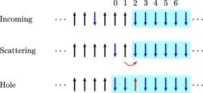
Figure 1: Schematic representation of the scattering of a particle with a domain wall. When the particle arrives at position 0, the jump to site 1 is forbidden by the control factor in (2). However, in this case the up spin at site 1 becomes mobile and it will start to propagate to the right. Eventually the domain wall gets replaced by 2 sites to the left, and the trajectory of the particle receives a displacement of 1 site to the right.

Interestingly, the domain wall does not contribute to the energy, but it has an effect on the dynamics due to the scattering displacement. The scattering event is shown schematically in Fig. 1.

We can also compute the situation with one particle and two domain walls, which is equivalent to having a particle and a bound state with a given number of down spins. For example if the bound state is of length two, we obtain the exact wave function

$${\left|\Psi\right\rangle}=\sum_{x=-\infty}^{0}e^{ipx}{\left|x,2,3\right\rangle}+\sum_{x=3}^{\infty}e^{ip(x-2)}{\left|0,1,x\right\rangle}.$$ (28)

The interpretation of the wave function is the following: originally the bound state of two DW’s occupies positions 2 and 3, and there is an incoming wave. Afterwards the bound state occupies positions 0 and 1 and the outgoing wave also suffers a displacement of 2 in the forward direction. This is shown in figure 2.

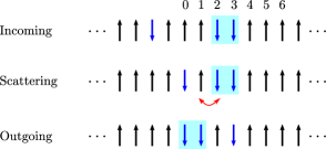
Figure 2: Scattering of a single particle and a length-2 bound state.

Notice that the hard core property is still satisfied, although it is not enforced, it is completely dynamical even in this case. This state also has energy $E=e(p)$, the two domain walls do not contribute.

The states (27) and (28) only exists in infinite volume, because the periodicity conditions can not be satisfied by them. However, the state (28) can be modified to fit into a finite volume situation with periodic boundaries. To this order we introduce a Fourier transform over the position of the block of 2 spins and write

$${\left|\Psi\right\rangle}=\sum_{y>x+1}e^{i(px+k(y-2))}{\left|x,y,y+1\right\rangle}\\ +\sum_{x>y+2}e^{i(p(x-2)+ky)}{\left|y,y+1,x\right\rangle}.$$ (29)

We can extract from this wave function the scattering phase

$$S_{p,2\text{DW}}(p,k)=e^{-2i(p-k)}.$$ (30)

The state (29) has energy $E=e(p)$ and it is periodic if $p$ and $k$ satisfy the equations

$$e^{ipL}S_{p,2\text{DW}}(p,k)=1,\qquad e^{ikL}S_{p,2\text{DW}}(k,p)=1.$$ (31)

Substituting (30) into the quantization conditions and introducing once again the total momentum $P=p+k$ we obtain

$$e^{ip(L-3)}=e^{-iP},\qquad e^{ik(L-3)}=e^{-iP}.$$ (32)

The domain walls do not contribute to the energy, but they modify the propagation of the free particles, and also the quantization conditions. The effect of the interaction is a change in the apparent length of the system by -3 and the appearance of the total momentum as a twist for the quantization conditions.

It turns out that this picture can be generalized to many body states: the model is integrable, and scattering of the particles among each other and on the domain walls leads to the same phases that we computed in this Section. In particular the scattering phase between a particle and a frozen block of spins of length $n$ does not depend on $n$.

The complete integrability of the model is most easily understood by considering a special connection to the XXZ spin chain, which we discuss in the next Section. The degeneracies resulting from the presence of the domain walls in generic states is discussed later in Section VIII.

IV Relation to the XXZ spin chain

Here we show that our model can be derived as a special limit of the XXZ spin chain. Our procedure is different from the one in Zadnik and Fagotti (2021); Zadnik et al. (2021), even though we also consider the large anisotropy limit.

The XXZ chain is given by the Hamiltonian

$$H=\sum_{j}\sigma^{x}_{j}\sigma^{x}_{j+1}+\sigma^{y}_{j}\sigma^{y}_{j+1}+\Delta(\sigma^{z}_{j}\sigma^{z}_{j+1}-1),$$ (33)

where $\Delta$ is the anisotropy parameter.

It is known that the XXZ chain is integrable, and it possesses a set of conserved charges that will be denoted as $\tilde{Q}_{\alpha}$. They satisfy

$$[\tilde{Q}_{\alpha},\tilde{Q}_{\beta}]=0.$$ (34)

The charge $\tilde{Q}_{\alpha}$ has an operator density that spans $\alpha$ sites; as usually $\tilde{Q}_{2}$ can be identified with the Hamiltonian, and $\tilde{Q}_{1}$ can be chosen as the global $S^{z}$ or alternatively as $Q_{1}$ written in (3).

The charges $\tilde{Q}_{\alpha}$ can be obtained either from a transfer matrix, or using the so-called boost operator Tetelman (55); Thacker (1986); Grabowski and Mathieu (1995); we describe here the latter method. The boost operator is defined as the formal expression

$$\mathcal{B}=i\sum_{j}j\tilde{h}_{j,j+1},$$ (35)

where $\tilde{h}_{j,j+1}$ is the Hamiltonian density acting on sites $j,j+1$. Then the charges are constructed through the recursive relations

$$\tilde{Q}_{\alpha+1}=[\mathcal{B},\tilde{Q}_{\alpha}].$$ (36)

Even though the r.h.s. is just a formal expression, the actual commutation relations result in a well defined extensive and local charge at each new step. This relation and the resulting charges were studied in detail in Grabowski and Mathieu (1994, 1995), where concrete formulas were given in a number of different cases. Furthermore, explicit formulas for $Q_{\alpha}$ with arbitrary $\alpha$ were derived in the recent works Nozawa and Fukai (2020); Nienhuis and Huijgen (2021).

We obtain our model by performing a special $\Delta\to\infty$ limit on the set of the conserved charges $\tilde{Q}_{\alpha}$. It can be seen from the boost relation that in the XXZ model the operators $\tilde{Q}_{\alpha}$ are polynomials in $\Delta$. Our main idea is to select the leading terms in $\Delta$ using a recursive procedure. Then the commutativity (34) will then ensure that our new charges $Q_{\alpha}$ also commute.

We start with $Q_{1}$ which does not depend $\Delta$, thus it will stay constant during the limit. The next charge is $\tilde{Q}_{2}$, which is the Hamiltonian (33). We select the leading piece in $\Delta$, which is (apart from the additive normalization, and stripping away the factor of $\Delta$) equal to $Q_{2}$ as given in (3). It is clear that $[Q_{1},Q_{2}]=0$. The charge $Q_{2}$ is not dynamical: the kinematical piece of the original $\tilde{Q}_{2}$ is scaled to zero, and only the “classical” part remains, which describes the classical Ising model. The disappearance of the dynamical terms in $Q_{2}$ prompts us to turn to the higher charges of the XXZ chain.

Therefore we take the explicit representation of $\tilde{Q}_{3}$ and $\tilde{Q}_{4}$ found in Grabowski and Mathieu (1995); Nozawa and Fukai (2020); Nienhuis and Huijgen (2021) and we select the leading terms in $\Delta$. It turns out that in the normalization of Grabowski and Mathieu (1995) the maximum power of $\Delta$ in $\tilde{Q}_{3}$ is linear, whereas it is quadratic in $\tilde{Q}_{4}$. Selecting these terms and stripping away the factors of $\Delta$ we obtain $Q_{4}$ and a new charge

$$\begin{split}Q_{3}&=\sum_{j}\frac{i}{4}(\sigma^{z}_{j}+\sigma^{z}_{j+3})(\sigma^{+}_{j+1}\sigma^{-}_{j+2}-\sigma^{-}_{j+1}\sigma^{+}_{j+2}).\end{split}$$ (37)

It is clear from the construction that all four charges commute with each other, because their commutativity is simply the leading order term from the relation (34). And $Q_{3}$ and $Q_{4}$ are already dynamical, even after the $\Delta\to\infty$ limit has been taken. The numerical pre-factors in $Q_{3}$ and $Q_{4}$ are added only for convenience, such that they have simple one-particle eigenvalues. Note that $Q_{3}$ is actually a three-site operator, it is just written conveniently in a four site representation as above.

Continuing to even higher charges we observe that more steps are needed. For example we find that the leading term in $\tilde{Q}_{5}$ is of order $\Delta^{2}$, and it is proportional to $Q_{3}$ as given above. Therefore a new charge can be obtained only if we subtract from $\tilde{Q}_{5}$ the appropriate multiple of $\tilde{Q}_{3}$ and then consider the leading term of the remainder. This procedure leads to a new operator $Q_{5}$ which commutes with all previous charges and which is given (after stripping away an irrelevant numerical pre-factor) as

$$\begin{split}Q_{5}=&\sum_{j}(\sigma^{z}_{j}+\sigma^{z}_{j+4})\Big{(}\sigma^{x}_{j+1}\sigma^{y}_{j+3}-\sigma^{y}_{j+1}\sigma^{x}_{j+3}\Big{)}\\ &+(\sigma^{z}_{j}+\sigma^{z}_{j+5})\Big{(}\sigma^{x}_{j+1}\sigma^{x}_{j+2}+\sigma^{y}_{j+1}\sigma^{y}_{j+2}\Big{)}\\ &\times\Big{(}\sigma^{y}_{j+3}\sigma^{x}_{j+4}-\sigma^{x}_{j+3}\sigma^{y}_{j+4}\Big{)}\\ &+(1+\sigma^{z}_{j}\sigma^{z}_{j+4})\sigma^{z}_{j+2}\Big{(}\sigma^{x}_{j+1}\sigma^{y}_{j+3}-\sigma^{y}_{j+1}\sigma^{x}_{j+3}\Big{)}.\end{split}$$ (38)

$Q_{5}$ appears to be a 6 site operator, but this is only apparent: after expanding the products it can be seen that every single term spans a maximum of 5 sites only. It follows from the construction that $Q_{5}$ commutes with all previous charges of our model. The charge $Q_{5}$ is identical to the operator $Q_{2}^{-}$ of Zadnik and Fagotti (2021), see formula (31) in that paper.

We can continue this recursive procedure to obtain the higher charges $Q_{\alpha}$ with $\alpha\geq 6$. The idea is always to focus on the leading terms in $\Delta$, and to subtract contributions that appeared in the earlier charges. We conjecture that this procedure leads to an infinite set of linearly independent charges $Q_{\alpha}$.

At present we do not have closed form results for the higher charges, and we do not have a direct transfer matrix construction for the new charges either. However, the existence of the charges $Q_{\alpha}$ with $\alpha=1\ldots 5$ is already enough to claim the integrability of the model. In fact, for integrability it is enough to have 2 independent dynamical conserved charges Kulish (1976), which in the present case are $Q_{3}$ and $Q_{4}$. The results of the works Nozawa and Fukai (2020); Nienhuis and Huijgen (2021) could be used to give explicit formulas for all the charges of our model, but this is beyond the scope of the present work.

We note a curious property of our construction: the boost relation (36) does not survive the $\Delta\to\infty$ limit. This is most easily seen from the relation between $Q_{2}$ and $Q_{3}$: whereas the original $\tilde{Q}_{3}$ is obtained from $\tilde{Q}_{2}$ using the boost, this is not true after the scaling. The new charge $Q_{2}$ is not dynamical, and it does not give $Q_{3}$ using the relation (36). However, we observe that the next relation is kept intact, which means that

$$Q_{4}\sim[\mathcal{B},Q_{3}]$$ (39)

with $\mathcal{B}$ given by the boosted $Q_{2}$. We comment further on this issue in the Conclusions.

IV.1 Bethe Ansatz for the XXZ chain

Here we present a summary of the Bethe Ansatz solution of the XXZ chain, which is well known Takahashi (1999). Our goal is to consider the $\Delta\to\infty$ limit of the full solution, this is presented below. Throughout this Section we will use the conventional parametrization

$$\Delta=\cosh(\eta).$$ (40)

It is known that the $N$-particle eigenstates of the XXZ model can be characterized by Bethe rapidities $\lambda_{j}$, $j=1\dots N$, that describe the one-particle momenta within the interacting states. The spin waves can form bound states, which are described by the so-called string solutions. The string hypothesis states that in the thermodynamic limit almost all eigenstates can be described by Bethe roots that organize themselves into the string patterns.

In our normalization $\lambda\in[-\pi/2,\pi/2]$ and the $n$-string propagation factors are

$$e^{ip_{n}(\lambda)}=\frac{1}{\Theta_{n/2}(\lambda)},$$ (41)

where we defined

$$\Theta_{n}(\lambda)=\frac{\sin(\lambda+in\eta)}{\sin(\lambda-in\eta)}.$$ (42)

The scattering of an $n$-string and an $m$-string is described by

$$\begin{split}&S_{n,m}=\begin{cases}\Theta_{|n-m|}\Theta^{2}_{|n-m|+2}\dots\Theta_{n+m}&\text{ for }n\neq m\\ \Theta^{2}_{2}\dots\Theta^{2}_{2n-2}\Theta_{2n}&\text{ for }n=m.\end{cases}\end{split}$$ (43)

Here we omitted the dependence on $\lambda$ in the notations.

We denote the string centers for the $n$-strings as $\lambda_{j,n}$. Then the approximate Bethe equations for the strings are

$$e^{ip_{n}(\lambda_{j,n})L}\mathop{\prod_{m,k}}_{(j,n)\neq(k,m)}S_{n,m}(\lambda_{j,n}-\lambda_{k,m})=1.$$ (44)

The energy of such an eigenstate is

$$\tilde{E}=2\sinh(\eta)\sum_{j,n}\tilde{h}_{2,n}(\lambda_{j,n})$$ (45)

where

$$\tilde{h}_{2,n}(\lambda)=\coth(-n\eta/2+i\lambda)-\coth(n\eta/2+i\lambda).$$ (46)

In a normalization dictated by the boost operator construction (see for example Section 3 of Pozsgay (2013)) the eigenvalues of $\tilde{Q}_{4}$ are

$$\tilde{Q}_{4}=(2\sinh(\eta))^{3}\sum_{j,n}\tilde{h}_{4,n}(\lambda_{j,n})$$ (47)

where

$$\tilde{h}_{4,n}(\lambda)=-\frac{\partial^{2}\tilde{h}_{2,n}(\lambda)}{\partial\lambda^{2}}$$ (48)

or with a more explicit formula

$$\tilde{h}_{4,n}(\lambda)=2\Big{[}\coth(n\eta/2+i\lambda)-\coth^{3}(n\eta/2+i\lambda)\\ -\coth(-n\eta/2+i\lambda)+\coth^{3}(-n\eta/2+i\lambda)\Big{]}.$$ (49)

IV.2 The special limit of the Bethe Ansatz

Here we consider the $\Delta\to\infty$ limit of the previous formulas. This particular limit of the XXZ chain was already studied in a series of works Bogoliubov and Malyshev (2011); Bogolyubov and Malyshev (2015). Also, it was known that in this limit the constrained XXZ chain can also be obtained Abarenkova and Pronko (2002); Trippe et al. (2010). However, the discussion of the dynamics under $Q_{4}$ is new.

First let us discuss the interpretation of the strings. It is known that in the $\Delta\to\infty$ limit the bound states become more and more bound Mossel and Caux (2010). Eventually in the strict $\Delta\to\infty$ limit an $n$-string will describe $n$ down spins placed beside each other. Thus it is natural in this special limit that the string solutions will correspond to the bound states in our model. Now we compute this correspondence, and the associated scattering phases.

We put forward that one limitation of this Bethe Ansatz picture is that it does not mirror the spin reflection symmetry of our model. As a consequence, the simple scattering state (27) of a particle and a DW is a very complicated object in this picture: the sea of down spins on the right would be described by an infinitely large string. In Section VI we present an alternative representation of the same model, where a single DW is treated as a separate particle. This picture will avoid some of the complications of the present description.

Now we compute the special limit of the eigenvalue functions. First of all we find that

$$\lim_{\Delta\to\infty}\tilde{h}_{2,n}(\lambda)=-2.$$ (50)

The explicit form of $Q_{2}$ given in (3) implies the limit

$$Q_{2}=\lim_{\Delta\to\infty}-\frac{H_{XXZ}}{2\Delta}$$ (51)

which together with (45) gives

$$h_{2,n}(\lambda)=2.$$ (52)

We see that the particles and the bound states give an equal contribution to $Q_{2}$, which does not depend on the momentum. This is clear from the actual form of $Q_{2}$, which shows sensitivity only to the domain walls.

Regarding the scaling of the $\tilde{Q}_{4}$ eigenvalues we find the large $\eta$ behaviour

$$\tilde{h}_{4,n}(\lambda)\approx-16e^{-n\eta}\cos(p),$$ (53)

where we identified $2\lambda=p$.

Combining with (47) and a re-scaling of $\tilde{Q}_{4}$ according to

$$Q_{4}=\lim_{\Delta\to\infty}\frac{\tilde{Q}_{4}}{64\Delta^{2}}$$ (54)

we get the scaling

$$h_{4,n}(p)=\lim_{\Delta\to\infty}\frac{(2\sinh(\eta))^{3}\tilde{h}_{4,n}(\lambda)}{64\Delta^{2}}$$ (55)

leading to

$$h_{4,n}(\lambda)=\begin{cases}-\cos(p)&\text{ for }n=1\\ 0&\text{ for }n>1.\end{cases}$$ (56)

This coincides with our real space computations in Section III.

Let us now consider the Bethe equations. Note that the limit of the functions $\Theta_{n}$ is simply

$$\Theta_{n}(\lambda)\quad\to\quad-e^{-ip},$$ (57)

where we identified $p=2\lambda$.

For the limit of the $S$-matrix factor between 1-strings we find simply:

$$S_{1,1}(p)=-e^{-ip}.$$ (58)

This agrees with the scattering phase found earlier in (15).

For the limit of the $S$-matrix factor between 1-strings and $n$-strings for $n>1$ we find:

$$S_{1,n}(p)=e^{-2ip}.$$ (59)

This is the same factor as found earlier in (30). We stress that this factor does not depend on $n$: the scattering phase is independent of the length of the bound state, it only depends on the number of domain walls crossed, which is two in this case.

We also compute the $S$-matrix between an $n$-string and an $m$-string with $n,m>1$. We find

$$S_{m,n}=\begin{cases}e^{-2mip}&\text{ for }n>m\\ -e^{-2nip}&\text{ for }n=m.\\ \end{cases}$$ (60)

Then we obtain the final Bethe equations

$$e^{ip_{j,n}L}\mathop{\prod_{m,k}}_{(j,n)\neq(k,m)}S_{n,m}(p_{j,n}-p_{k,m})=1.$$ (61)

For particles (or equivalently for 1-strings) the Bethe equations take a particularly simple form. Using the above results we get

$$e^{ip_{j,1}L}\prod_{k\neq j}-e^{-i(p_{j,1}-p_{k,1})}\prod_{m=2,3,\dots}\prod_{k}e^{-2i(p_{j,1}-p_{k,m})}=1.$$ (62)

This is then rewritten as

$$e^{ip_{j,1}(L-N_{1}-2N_{s})}=(-1)^{N_{1}-1}e^{-iP_{1}}e^{-2iP_{s}},$$ (63)

where we introduced the total string number (without the particles)

$$N_{s}=N_{2}+N_{3}+\dots$$ (64)

and

$$P_{1}=\sum_{j}p_{j,1},\qquad P_{s}=\sum_{m=2,3,\dots}\sum_{k}p_{k,m}.$$ (65)

We see that for the quantization condition of these particles the various strings are grouped together, such that the information on the string length disappears. Only the total number of the strings and their total momentum enters the equations. This is perfect agreement with other descriptions of the model which will be discussed below.

The energy of the states is

$$E=\sum_{j}e(p_{j,1})+\mu(N_{1}+N_{s})\\ +h\left[N_{1}+\sum_{m=2,3,\dots}mN_{m}\right].$$ (66)

We observe that degeneracies between different string lengths remain if $h=0$. This is discussed in more detail below in VIII.

V Boundary conditions

In this Section we investigate the model with open boundaries; this is the case that was originally considered in Yang et al. (2020). We will show that the boundary problem is even simpler than the periodic one: it gives simpler Bethe equations, we can easily prove completeness of the Bethe Ansatz, and the study of the thermodynamics is also easier (see Section X).

This simplicity can be explained by a standard semi-classical picture. We consider the motion of the particles in a finite volume, both in the periodic and in the boundary case. In the periodic case the particles move along the chain and eventually travel around the full volume. In this process every particle hits every DW one time, therefore the domain walls are displaced. This process is then repeated over time, thus the DW’s can not have fixed positions. In contrast, in the boundary case the particles travel back and forth between the left and right boundaries. In this process every particle hits every DW one time from the left and one time from the right, and the displacements of the DW’s add up to zero. In other words the DW’s stay in their original positions as the particles finish a full cycle of traversing the available volume. This means that in the boundary case we can label the states with the DW positions and the particle momenta. This phenomenon shows that the open boundary condition is ”more compatible” with the bulk scattering than the periodic one.

In the boundary setting the Hamiltonian of a chain of length $L+2$ is

$$H=-\frac{1}{4}\sum_{j=0}^{L-1}\left(1+\sigma_{j}^{z}\sigma_{j+3}^{z}\right)\left(\sigma_{j+1}^{+}\sigma_{j+2}^{-}+\sigma_{j+1}^{-}\sigma_{j+2}^{+}\right).$$ (67)

This Hamiltonian can be obtained from a double row transfer matrix (using the identity as the so-called $K$-matrices) of the XXZ spin chain in the same way as for the periodic case (see section IV). Using the same argument as section IV we can convince ourselves that the Hamiltonian is integrable. We will not treat this procedure in detail here, and for the algebraic framework of the boundary XXZ chain we refer the reader to Sklyanin (1988).

The following charges are also conserved for open boundaries

$$Q_{1}=\sum_{j=0}^{L+1}\sigma_{j}^{z},\qquad Q_{2}=\sum_{j=0}^{L}\sigma_{j}^{z}\sigma_{j+1}^{z}.$$ (68)

In addition, specific to the boundary case, we have the following conserved charges

$$B_{l}=\sigma_{0}^{z},\qquad B_{r}=\sigma_{L+1}^{z}.$$ (69)

We see that the first and the last sites are not dynamical and the Hilbert space is decomposed as $\mathcal{H}=\mathcal{H}_{\uparrow\uparrow}\otimes\mathcal{H}_{\uparrow\downarrow}\otimes\mathcal{H}_{\downarrow\uparrow}\otimes\mathcal{H}_{\downarrow\downarrow}$ where

$$\mathcal{H}_{\uparrow\uparrow} =\mathrm{span}\left\{\left|\uparrow,\dots,\uparrow\right\rangle\right\}, \mathcal{H}_{\uparrow\downarrow} =\mathrm{span}\left\{\left|\uparrow,\dots,\downarrow\right\rangle\right\},$$

$$\mathcal{H}_{\downarrow\uparrow} =\mathrm{span}\left\{\left|\downarrow,\dots,\uparrow\right\rangle\right\}, \mathcal{H}_{\downarrow\downarrow} =\mathrm{span}\left\{\left|\downarrow,\dots,\downarrow\right\rangle\right\}.$$ (70)

Each subspace has dimension $2^{L}$. In the following we focus on the subspace $\mathcal{H}_{\uparrow\uparrow}$. The other sectors can be analyzed similarly.

V.1 Bethe Ansatz

In this subsection we present the characterization of the spectrum of $\mathcal{H}_{\uparrow\uparrow}$. Let us start with the one-magnon state. The Bethe Ansatz eigenstate reads

$$\left|\Psi\right\rangle=\sum_{x=1}^{L}\left(e^{-ipx}+R(p)e^{ipx}\right)\left|x\right\rangle.$$ (71)

We can calculate the energy, the reflection factor $R(p)$ and the Bethe Ansatz equation in the usual way, which leads to

$$e(p) =-\cos(p),$$ (72)

$$R(p) =-1,$$ (73)

$$e^{-2ip(L+1)} =1.$$ (74)

Solutions to be Bethe equation are

$$p=\pi\frac{n}{L+1},\qquad n=1,\dots,L.$$ (75)

The number of solutions agrees with the dimension of the one-magnon subspace of $\mathcal{H}_{\uparrow\uparrow}$.

We can generalize this Ansatz to general states. We learned from the periodic case that the spectrum contains magnons and DW’s. The width of the DW’s have to be at least two since the one distance means there is a hole excitation which will be transformed to a magnon at some point.

There is now a key difference as opposed to the periodic case; above we have already touched upon this issue when discussing the semi-classical picture. In the boundary setting we can have bound states with fixed positions, up to the scattering displacements with the particles. In contrast, in the periodic case we needed a Fourier transform over the bound state positions such as in (29), otherwise there was no way to satisfy the periodicity conditions. At the heart of this problem lies the periodic property itself, which makes it impossible to identify which particle is to the left or to the right as compared to any other particle. In the boundary setting this is clearly possible, and we can assign well defined positions to the DW’s, which are changed only as a result of the scattering with the particles.

Now we present the construction of the Bethe states. We present the final results without proofs; the form of the wave functions follow from the previous results given above. A long and detailed proof would not contribute considerably to the understanding of the model. However, to avoid simple mistakes we checked the wave functions below in small volumes and found that they indeed produce the eigenstates of the boundary model.

The wave functions of the $N$ particle states without DW’s are

$$|\mathbf{p}_{N}\rangle=\sum_{x_{1}<\dots x_{N}}\chi(\mathbf{x},\mathbf{p})|x_{1},x_{2}+1,x_{3}+2,\dots x_{N}+N-1\rangle$$ (76)

where

$$\chi(\mathbf{x},\mathbf{p})=\sum_{\sigma\in\mathcal{S}_{N}}\sum_{s_{j}=\{-,+\}}\mathrm{sgn}(\sigma)\left[\prod_{j=1}^{N}s_{j}\right]e^{i\sum_{i=1}^{N}s_{i}p_{\sigma(i)}x_{i}}.$$ (77)

The summation over the signs $s_{j}$ correspond to whether the particle is moving from the left boundary to the right one or vice versa.

Going further we can also insert bound states into the chain, which will be displaced as particles scatter on them. Such states will thus be given by a complicated summation over the various possibilities for the positions of the particles. In any case the states can be labeled by the positions of the DW’s as the particles occupy the leftmost possible positions. Thus we can label the states with domain walls at positions $(x_{i},y_{i})$ for $i=1,\dots,M$ as

$$|\mathbf{p}_{N},\mathbf{x}_{M},\mathbf{y}_{M}\rangle\approx\\ |1,3,\dots,2N-1,x_{1},x_{1}+1,\dots,y_{1},\dots,x_{M},\dots y_{M}\rangle+\dots{}$$ (78)

where $y_{i}-x_{i}\geq 2$, $x_{i+1}-y_{i}\geq 2$, and the dots stand for other components of the wave function.

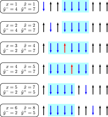
Figure 3: Illustration of effective position $x$ and real positions $\tilde{x},\tilde{y}^{\pm}$.

To describe the full wave function with $N$ particles and $M$ DW’s it is best to consider the motion of $N$ free fermions in a box with effective length $\tilde{L}=L+1-N-2M$. It is convenient to use effective positions $1\leq x_{1}<\dots<x_{N}\leq\tilde{L}$ and real positions $1\leq\tilde{x}_{1}<\dots<\tilde{x}_{N}\leq L$. The effective position is the position of the particle in the auxiliary free fermion picture and the real position is its actual position. Ignoring the DWs we saw that the connection between real and effective positions is $\tilde{x}_{k}=x+k-1$ (see (76)) which is a manifestation of the hard rod property (see also Section XIII).

We also saw that the DWs are displaced by the scattering. Let $(\tilde{y}_{j}^{+},\tilde{y}_{j}^{+})$ be the position of the DW when the effective positions are $\{x_{k}\}$. Figure 3 shows the connections between these positions if we have one particle and one bound state. We can see that the real position is increased by one when the particle reaches the left of the domain wall and one more when it reaches the right. We can also see that $\tilde{y}^{-}$ and $\tilde{y}^{+}$ are decreased by two when the particle reaches the left and right respectively.

Having more particles and bound states we have to count how many particles reached a DW to get the real positions of given effective positions. If the $k$th particle reaches the left of $j$th DW then the $k+1,\dots,N$ particles have to already reached it therefore its position when the $k$th particle reaches it is $\tilde{y}^{-}_{l}=y^{-}_{l}-2(N-k)$. The $k$th particle can reach left of $j$th DW only when it already went through $1,\dots,j-1$ bound states therefore its real position is $\tilde{x}_{k}=x_{k}+k-1+2(j-1)$ therefore the $k$th particle pasted the left of the $j$th DW if $x_{k}-y_{j}^{-}+2N-k+2j-2\geq 0$. In an analogous way the $k$th particle is pasted the right of the $j$th DW if $x_{k}-y_{j}^{+}+2N-k+2j-1\geq 0$.

In summary the full wave function can be written as

$$|\mathbf{p}_{N},\mathbf{y}_{M}^{-},\mathbf{y}_{M}^{+}\rangle=\sum_{1\leq x_{1}<\dots x_{N}\leq\tilde{L}}\chi(\mathbf{x},\mathbf{p})|\tilde{\mathbf{x}}_{N},\tilde{\mathbf{y}}_{M}^{-},\tilde{\mathbf{y}}_{M}^{+}\rangle,$$ (79)

where $\tilde{L}=L+1-N-2M$, $y_{i}^{+}-y_{i}^{-}\geq 2$, $y_{i+1}^{-}-y_{i}^{+}\geq 2$,

$$\tilde{x}_{k} =x_{k}+k-1+\sum_{j=1}^{M}\Bigl{(}\Theta(x_{k}-y_{j}^{-}+2N-k+2j-2),$$

$$\qquad\qquad\qquad+\Theta(x_{k}-y_{j}^{+}+2N-k+2j-1)\Bigr{)},$$ (80)

$$\tilde{y}_{j}^{-} =y_{j}^{-}-2\sum_{k=1}^{N}\Theta(x_{k}-y_{j}^{-}+2N-k+2j-2),$$ (81)

$$\tilde{y}_{j}^{+} =y_{j}^{+}-2\sum_{k=1}^{N}\Theta(x_{k}-y_{j}^{+}+2N-k+2j-1),$$ (82)

($\Theta$ is the unit-step function) and

$$|\mathbf{x}_{N},\mathbf{y}_{M}^{-},\mathbf{y}_{M}^{+}\rangle=\left[\prod_{i=1}^{N}\sigma_{x_{i}}^{x}\right]\left[\prod_{i=1}^{M}\prod_{j=0}^{y_{i}^{+}-y_{i}^{-}}\sigma_{y_{i}^{-}+j}^{-}\right]|0\rangle.$$ (83)

We can now easily calculate the Bethe equations for the particles. Let us pick up a particle and move it through the chain. It will hit every other particle and bound state two times. The single time scattering phases are $-e^{-i(p_{j}\mp p_{k})}$ and $-e^{-2ip_{j}}$ for magnons and bound states. We can see that the momenta $p_{k}$ drop out from the Bethe equations since the products of the scattering phases are $e^{-i(p_{j}-p_{k})}e^{-i(p_{j}+p_{k})}=e^{-i2p_{j}}$, and therefore the Bethe equations are

$$e^{2ip_{j}(L-N-2M+2)}=1,$$ (84)

where $N$ and $M$ are the number of the magnons and the bound states. We can see that the Bethe equations are decoupled and they are the same as the one magnon Bethe equation with length $\tilde{L}=L+1-N-2M$. Therefore we obtained an effectively free theory with a modified volume.

We can check that the above defined states span the entire Hilbert space $\mathcal{H}_{\uparrow\uparrow}$. Fixing the number of particles and bound states it is obvious that we can place the bound states in several ways. The number of these possibilities is

$$\mathrm{DW}(L,N,M)=\binom{L-2N+2-2M}{2M}.$$ (85)

The effective length for the magnons is $\tilde{L}=L+1-N-2M$, therefore the number of the solutions of the Bethe equations is

$$\mathrm{BA}(L,N,M)=\binom{L+1-N-2M}{N}.$$ (86)

From (85) and (86) we can count number of states we described above

$$\Sigma(L)=\sum_{N=1}^{(L+1)/2}\sum_{M=1}^{(L-2N+2)/4}\mathrm{DW}(L,N,M)\mathrm{BA}(L,N,M).$$ (87)

We can convince ourselves that

$$\Sigma(L)=2^{L}=\dim\mathcal{H}_{\uparrow\uparrow}.$$ (88)

We can see that we created as many states as the dimension of the Hilbert space. We checked numerically that the free Bethe equations above with the bound state degeneracies as given above produce the complete spectrum of the open spin chain up to $L=8$.

VI Bond-site transformation

The goal of this Section is to build a different representation of the same model, such that the standalone Domain Walls can be interpreted as particles (of a new particle species). We perform a non-local transformation: we put dynamical variables on the bonds between sites, and build a dynamical model for the bonds. It turns out that our original charges $Q_{4}$ and $Q_{2}$ can be represented by local operators after the transformation. The advantage of such a representation is that it leads to a simpler Bethe Ansatz description, with only two particle types. This Bethe Ansatz naturally respects the spin reflection invariance of the original model. However, the advantages come at a cost: the original charge $Q_{1}$ becomes a non-local operator in the new basis.

We put variables onto the bonds (links) between the sites, and we perform a change of basis from the old computational basis to the new one. We have two options for each link, which we denote by $\circ$ and $\bullet$. We put $\circ$ if the two neighbours are of the same spin, and we put $\bullet$ if the two neighbours are different. This transformation is completely invariant with respect to a global spin flip, which is an invariance of the operators $Q_{2}$ and $Q_{4}$. This transformation is identical to the one used in Zadnik and Fagotti (2021); Zadnik et al. (2021) to derive their dual Hamiltonian; this is most easily seen from footnote 4 on page 11. of Zadnik and Fagotti (2021), where the transformation rule for the $\sigma^{z}$ operators is given. The interpretation as a bond model is new.

We can define this bond model on a periodic lattice, but for simplicity we first consider the boundary setting. We consider the sector of the original model where the spin at site $j=1$ is in the up spin position. Then we construct the bond basis for the $L^{\prime}=L-1$ bonds, without any restriction on the last site. This way the Hilbert space will have a dimension of $2^{L^{\prime}}$.

Let us now give the operator representation of the charges in the bond basis. In terms of spins, we can interpret ${\left|\circ\right\rangle}$ as the up spin, and ${\left|\bullet\right\rangle}$ (the particle) as the down spin, and below we will use the Pauli matrices in this new basis accordingly.

Under this transformation the charges $Q_{2,3,4}$ become the local operators

$$\begin{split}Q^{B}_{2}&=\sum_{j=1}^{L^{\prime}}\frac{1-\sigma^{z}_{j}}{2},\\ Q^{B}_{3}&=\frac{i}{2}\sum_{j=1}^{L^{\prime}-1}\left(\sigma^{+}_{j}P^{\bullet}_{j+1}\sigma^{-}_{j+2}-\sigma^{-}_{j}P^{\bullet}_{j+1}\sigma^{+}_{j+2}\right),\\ Q^{B}_{4}&=\frac{1}{2}\sum_{j=1}^{L^{\prime}-1}\sigma^{-}_{j}P^{\bullet}_{j+1}\sigma^{+}_{j+2}+\sigma^{+}_{j}P^{\bullet}_{j+1}\sigma^{-}_{j+2},\end{split}$$ (89)

where $P^{\bullet}_{j}$ is the projector onto the state ${\left|\bullet\right\rangle}$ on site $j$. This form of the charges is obtained by direct computation. They were already given in Zadnik and Fagotti (2021); Zadnik et al. (2021) using a transformation on the level of the operators.

Interestingly, we can build the non-Hermitian combinations $Q^{B}_{4}\pm iQ^{B}_{3}$, that describe propagation terms towards the left or to the right only.

A disadvantage of the bond picture is that $Q_{1}$ given in (3) is not a local operator anymore. Instead, it is given by the highly non-local expression

$$Q^{B}_{1}=\frac{1}{2}\sum_{j=1}^{L^{\prime}}\left[1-\prod_{k=1}^{j}\sigma^{z}_{j}\right].$$ (90)

As noted earlier, we can also define the bond model with the operators above, assuming periodic boundary conditions. In this case the bond model is not completely equivalent to the original spin chain: for example, it allows the presence of an odd number of domain walls, which were forbidden by definition in the old chain. Nevertheless, the sectors with an even number of DW’s are equivalent to those of the original chain. In these sectors every state of the bond model actually describes two different states from the original chain, which are related by spin reflection.

Sectors of the bond model with an odd number of DW’s can be accommodated in the original spin chain if twisted boundary conditions are chosen, with a twist given by spin reflection. Such a model is also interesting on its own right Batchelor et al. (1995); Yung and Batchelor (1995), but we do not discuss it here.

VI.1 Dynamics and Bethe Ansatz in the bond picture

In the bond picture a single $\bullet$ represents an original DW, while two bullets on neighbouring sites represent an original particle. Correspondingly, the kinematical terms in $Q^{B}_{3}$ and $Q^{B}_{4}$ move the double bullets, but they leave the single $\bullet$ invariant. To be more precise, the only non-vanishing matrix elements of $Q^{B}_{3}$ and $Q^{B}_{4}$ are those corresponding to the moves

$${\left|\circ\bullet\bullet\right\rangle}\to{\left|\bullet\bullet\circ\right\rangle},\qquad{\left|\bullet\bullet\circ\right\rangle}\to{\left|\circ\bullet\bullet\right\rangle}.$$ (91)

We can regard the DW as the fundamental excitation, and the original particle (the doublet $\bullet\bullet$) as a bound state of two DW’s. The phenomenon that a single excitation is stable but a bound state of two excitations is dynamical is similar to the situation in fracton models (see the reviews Nandkishore and Hermele (2019); Pretko et al. (2020)).

Let us now construct the Bethe Ansatz wave functions in the bond model. We set $h=0$ (thus we discard the non-local charge $Q_{1}^{B}$) and consider the local Hamiltonian

$$H^{B}=Q^{B}_{4}+\mu Q^{B}_{2}.$$ (92)

with periodic boundary conditions. The construction below is not rigorously proven: we construct the Bethe Ansatz by assuming factorized scattering and using the $S$-matrix factors extracted from the two body problem. We put forward that the Bethe Ansatz is not unique: different constructions lead to different choices for the basis vectors in the highly degenerate subspaces. We discuss this issue at the end of this Section.

We have two types of excitations in the model: the single $\bullet$ which is a DW, and the $\bullet\bullet$ which is a particle. We will use the notations $p$ and $DW$.

Correspondingly we introduce local creation operators

$$A^{a}_{j}=\begin{cases}\sigma^{-}_{j}&\text{ if }a=DW\\ \sigma^{-}_{j}\sigma^{-}_{j+1}&\text{ if }a=p.\\ \end{cases}$$ (93)

Note that we have automatic exclusions:

$$A^{p}_{x}A^{p}_{x+1}=A^{p}_{x}A^{DW}_{x+1}=0.$$ (94)

Let us consider a state with $N$ particles and $M$ DW’s; the set of the particle and DW momenta will be denoted as ${\boldsymbol{p}}_{N}$ and ${\boldsymbol{k}}_{M}$. The wave function is most easily written down by merging these sets. Therefore we introduce a set of momenta ${\bf q}_{N^{\prime}}$ and a set of particle types ${\bf a}_{N^{\prime}}$ with $N^{\prime}=N+M$. We assume that there are no coinciding rapidities.

The wave function is then written as

$$\begin{split}{\left|\Psi\right\rangle}=\sum_{x_{1}\leq x_{2}\leq\dots\leq x_{N^{\prime}}}\sum_{\mathcal{P}\in S_{N^{\prime}}}e^{i\sum_{j=1}^{N^{\prime}}q_{\mathcal{P}_{j}}x_{j}}\\ \times\mathop{\prod_{j<k}}_{\mathcal{P}_{j}>\mathcal{P}_{k}}S_{a_{j},a_{k}}(q_{j},q_{k})\prod_{j=1}^{N^{\prime}}A^{a_{\mathcal{P}_{j}}}_{x_{j}}{\left|\emptyset\right\rangle}.\end{split}$$ (95)

The scattering factors for different particle pairs are:

$$\begin{split}S_{DW,DW}(q_{1},q_{2})&=S_{p,p}(q_{1},q_{2})=-e^{-i(q_{1}-q_{2})},\\ S_{p,DW}(q_{1},q_{2})&=e^{-i(q_{1}-2q_{2})}.\end{split}$$ (96)

For simplicity we assume that the original ordering of particle types is $2,2,2,\dots,2,1,1,1,\dots,1$.

Note that the $S$-matrix is such that for DW’s the occupation of neighbouring sites is forbidden. This ensures that we do not mistake two domain walls close-by with a particle. Also, if we have two particles at positions $x_{1}<x_{2}$, then $x_{2}=x_{1}+1$ is forbidden by the action of the creation operators, but the next possibility $x_{2}=x_{1}+2$ is allowed. Furthermore, if we have a DW at $x_{1}$ and a particle at $x_{2}$ then $x_{2}=x_{1}+1$ is allowed, but the other ordering $x_{1}=x_{2}+1$ is forbidden. Thus, in this wave function a sequence of ${\left|\bullet\bullet\bullet\right\rangle}$ embedded in the vacuum is interpreted as a DW and a particle from the left to the right. It is merely a choice which follows from our definition of the creation operators.

The energy of this state is

$$E=\mu N_{DW}+\sum_{a_{j}=p}(e(p_{j})+2\mu).$$ (97)

The sum runs over the particles only. The domain walls only contribute to the energy through the chemical potential $\mu$.

The Bethe equations for the $p$ and $k$ variables are

$$\begin{split}e^{ip_{j}L}\mathop{\prod_{l=1}^{N}}_{l\neq j}S_{p,p}(p_{j},p_{l})\prod_{m=1}^{M}S_{p,DW}(p_{j},k_{m})&=1,\\ e^{ik_{l}L}\mathop{\prod_{m=1}^{M}}_{m\neq l}S_{DW,DW}(k_{l},k_{m})\prod_{j=1}^{N}S_{DW,p}(k_{l},p_{j})&=1.\end{split}$$ (98)

Substituting the factors we get

$$\begin{split}e^{ip_{j}(L-N-M)}e^{iP}e^{2iK}&=(-1)^{N-1},\\ e^{ik_{l}(L-2N-M)}e^{iK}e^{iP}&=(-1)^{M-1},\end{split}$$ (99)

where we defined

$$P=\sum_{j=1}^{N}p_{j},\qquad K=\sum_{j=1}^{M}k_{j}.$$ (100)

The energy is carried only by the particles, and the effect of the domain walls is only a change in the available volume. Correspondingly, the actual values of the $k_{j}$ variables do not matter for the particle momenta $p_{j}$, which is influenced only by the sum $K$. Thus the distribution of $K$ among the variables $k_{j}$ only contributes to the degeneracies of the energy levels. This can be seen more explicitly by taking the product of the second set of equations, which leads to the following coupled equations for the variables $p_{j}$ and $K$:

$$\begin{split}e^{ip_{j}(L-N-M)}e^{iP}e^{2iK}&=(-1)^{N-1},\\ e^{iK(L-2N)}e^{iPM}&=1,\end{split}$$ (101)

Explicit solutions to the equations above are found as follows. The overall momenta are expressed as

$$\begin{split}&P\frac{L(L-M-2N)}{(L-2N)}\\ &=\pi\left(N-1-\frac{2M(M-1)}{L-2N}\right)N+2\pi I-4\pi\frac{JN}{L-2N},\end{split}$$ (102)

and

$$K=\frac{\pi(M-1)M+2\pi J-PM}{L-2N},$$ (103)

where $I$ and $J$ are arbitrary integers. Afterwards the particle momenta $p_{j}$ are expressed as

$$p_{j}=\frac{(N-1+2I_{j})\pi-P-2K}{L-N-M},$$ (104)

where quantum numbers $I_{j}$ are given by $I=\sum_{s=1}^{N}I_{s}$: $0<I_{1}<I_{2}\dots<I_{N}<L$.

Let us compare these equations with (59) that was derived using the strings of the XXZ model. We can see in (59) that the contribution to the volume change is the same for every string, thus for every bound state. In the bond picture this means that the volume change does not depend on the relative position of the DW’s, just their total number. This is consistent with the equations above. However, the “twist” felt by the particles depends on the momentum of the DW’s.

This basis is certainly different from the one obtained by the string picture in the original model. The key difference is that here the DW’s are allowed to move independently, whereas in the string picture the two DW’s of the bound state are always at a fixed distance. Both pictures describe highly degenerate energy levels, and such differences only amount to a free choice of the basis.

In fact, it is easy to see that the Bethe states obtained in this bond picture can not be identical to those of the original model. This happens because in the bond picture the two DW’s associated to an original string solution can not have the same momenta, therefore they can not move together. Furthermore, the wave function (95) naturally gives a linear combination of states where the “string lengths” vary. States with fixed string lengths are not reproduced by this formula. However, we stress that the two descriptions merely correspond to two different choices for the basis vectors in a highly degenerate eigenspace.

It is worth mentioning that the Bethe Ansatz solution presented above is completely different from the one of Zadnik and Fagotti (2021); Zadnik et al. (2021), and it is not straightforward to find a dictionary between the two solutions, and most probably they lead to different basis vectors in the highly degenerate eigenspaces. We checked by numerical computations that both constructions correctly reproduce the spectrum up to $L=8$.

VII Non-local mapping to the $SU(3)$ XX model

Here we show that the bond model can be mapped to the Maassarani-Mathieu (MM) spin chain, which is also known as the $SU(N)$ XX model Maassarani and Mathieu (1998); our mapping concerns the $SU(3)$-related case. The mapping is similar in spirit to the non-local mapping between the phase model and the XX model which first appeared in Bogoliubov and Timonen (2011) and which was treated detail in Pozsgay and Eisler (2016). The mapping for the present model is new, and it is different from the connection with the Bariev model Bariev (1991) found in Zadnik and Fagotti (2021).

We start with the bond model with length $L$ in the boundary setting. This model will be mapped to a spin chain with local dimension 3, with local basis states denoted as ${\left|1\right\rangle}$, ${\left|2\right\rangle}$ and ${\left|3\right\rangle}$. As before, we construct the mapping on the level of the basis states. We will see that the mapping is volume changing: different states are mapped to states of the new model with different lengths.

The rules for the mapping in the computational basis are as follows. We represent each basis state as a sequence of $\bullet$’s and $\circ$’s. We proceed from the left to the right of this sequence and we translate it to a new sequence consisting of the numbers $1,2,3$. If at a given position we encounter a $\circ$ then we add a $1$ to the new sequence. Then we move further to the next entry. If we encounter a $\bullet$ then we also need to check the next entry: a pair $\bullet\bullet$ is then mapped to $2$, whereas the pair $\bullet\circ$ is mapped to $3$. This rule is then applied as we proceed along the chain.

This mapping works flawlessly on a half-infinite chain, but it runs into a problem on a finite chain if the last entry is a single $\bullet$ for which no rule is specified. Here we are not concerned with the boundary conditions, we are focusing on the mapping on the bulk, thus we discard this problem. It is possible that an exact mapping with open boundary conditions could be constructed, but we leave this problem to a future work.

The mapping backwards is more easily summarized as

$${\left|1\right\rangle}\to{\left|\circ\right\rangle},\qquad{\left|2\right\rangle}\to{\left|\bullet\bullet\right\rangle},\qquad{\left|3\right\rangle}\to{\left|\bullet\circ\right\rangle}.$$ (105)

Let us discuss the changes in the length. If the numbers of the components $1,2$ and $3$ in the new sequence are given by $N_{1,2,3}$, with the total length being

$$L^{\prime}=N_{1}+N_{2}+N_{3},$$ (106)

then the length of the original chain is

$$L=N_{1}+2N_{2}+2N_{3}.$$ (107)

We see that different basis states of our model are mapped to MM chains with different length. It is useful to note that the original particle and DW numbers are

$$N=N_{2},\qquad M=N_{3},$$ (108)

thus the volume of the MM chain for a given $N,M$ reads

$$L^{\prime}=L-N-M.$$ (109)

We focus on the Hamiltonian in the bond model given by $Q^{B}_{4}$ in (89), which results in the transition rules (91). It can be checked that after the basis transformation this translates into the transition matrix elements

$${\left|12\right\rangle}\leftrightarrow{\left|12\right\rangle},\qquad{\left|23\right\rangle}\leftrightarrow{\left|23\right\rangle}.$$ (110)

We also write down the Hamiltonian that encodes these transitions. Let $E^{a,b}_{j}$ with $a,b=1\dots 3$ be the elementary matrices that contain a single 1 in row $a$ and column $b$, acting on the local Hilbert space on site $j$ of the new model. Then the MM Hamiltonian is Maassarani and Mathieu (1998)

$$H_{\rm MM}=-\frac{1}{2}\sum_{j=1}^{L^{\prime}}\sum_{a=1}^{2}\left[E^{a,a+1}_{j}E^{a+1,a}_{j+1}+E^{a+1,a}_{j}E^{a,a+1}_{j+1}\right].$$ (111)

This is now written down for periodic boundary conditions and we included a factor of -1/2 to match our previous normalizations. We note that this model is also equivalent to the infinite interaction limit of the Hubbard model (also known as the t-0 model), see for example Göhmann and Murakami (1998); Essler et al. (2005).

It is useful to consider the specific sector of the bond model, which includes only particles. This sector is equivalent to the constrained XXZ model treated in Sec. II.1. Applying the non-local mapping to this sector we see that only the local states $1$ and $2$ are populated. In this sector the MM chain is equivalent to the standard XX model. In Pozsgay and Eisler (2016) it was shown that the so-called phase model is equivalent to the XX model by a similar non-local transformation. We have thus obtained three different models that are equivalent to each other via the non-local mapping.

We stress that the equivalence of these models is established only for the bulk, because generally the boundary conditions spoil the mapping. This situation is analogous to the one treated in Pozsgay and Eisler (2016). As mentioned above, an exact mapping could be found perhaps with open boundary conditions, but we do not pursue this direction here.

We now briefly discuss the spectrum of the MM Hamiltonian (111) with periodic boundary conditions, and the construction of its eigenstates through Bethe Ansatz. An algebraic treatment was presented in Maassarani and Mathieu (1998), and here we discuss the coordinate Bethe Ansatz solution. In fact we will see that there are two different constructions, which are related to each other by a particle-hole transformation.

The first version of the coordinate Bethe Ansatz is close in spirit to the usual nested Bethe Ansatz, where we start with a chosen reference state and build excitations above it, such that the orientation of the excitations will involve the “nesting”, or second Bethe Ansatz. We start with the sector where only the local states ${\left|1\right\rangle}$ and ${\left|2\right\rangle}$ are populated; in this sector the MM model is equivalent to the standard XX model. The eigenstates in this sector are therefore constructed as excitations on top of the pseudo-vacuum ${\left|\rm vac\right\rangle}={\left|2\ldots 2\right\rangle}$. They are parameterized by a set of momenta $\mathbf{k}=\{k_{1},\ldots k_{N}\}$, and take the form

$${\left|\mathbf{k}\right\rangle}=\sum_{x_{1}<\ldots<x_{N}}\sum_{\mathcal{P}\in\mathfrak{S}_{N}}\mathrm{sgn}(\mathcal{P})e^{i\sum_{j=1}^{N}k_{\mathcal{P}_{j}}x_{j}}{\left|1_{x_{1}}\ldots 1_{x_{N}}\right\rangle}\,,$$ (112)

where we have used the notation ${\left|1_{x_{1}}\ldots 1_{x_{N}}\right\rangle}=E_{j_{1}}^{2,1}\ldots E_{j_{n}}^{2,1}{\left|\rm vac\right\rangle}$. Periodicity of the wave function then imposes the quantization condition $e^{ik_{j}L^{\prime}}=(-1)^{N-1}$ for each $j$, and for a given value of $N$ the momenta $k_{1},\ldots k_{N}$ may take any of the $L$ distinct values compatible with this condition, provided that they are all distinct. The corresponding energies are given by

$$E=\sum_{j=1}^{N}\cos(k_{j}).$$ (113)

Turning to more general sectors, that is, with $N_{3}\neq 0$, we introduce the states ${\left|\mathbf{k}^{\alpha_{1},\ldots,\alpha_{N}}\right\rangle}$, with $\alpha_{j}\in\{1,3\}$. These have the same form as (112), but where the sequence $1_{x_{1}}\ldots 1_{x_{N}}$ is replaced by the corresponding sequence of 1s and 3s (we then have $N=N_{1}+N_{3}$). Since the order of 1s and 3s along the chain is not modified by the transition matrix elements (110), the states ${\left|\mathbf{k}^{\alpha_{1},\ldots,\alpha_{N}}\right\rangle}$ are locally eigenstates of the MM Hamiltonian, with energies again given by (113). However, on a chain of finite size requiring periodicity of the wave function mixes states with sequences ${\alpha_{1},\ldots,\alpha_{N}}$ related through cyclic permutations. We therefore construct eigenstates as linear combinations of the form

$$\sum_{n=1}^{N}e^{iqn}{\left|\mathbf{k}^{U^{n}(\alpha_{1},\ldots,\alpha_{N})}\right\rangle}\,,$$ (114)

where $U$ cyclically permutes the indices $\alpha_{i}$. The pseudo-momentum $q$ is quantized through $e^{iqN}=1$, but depending on the sequence $\alpha_{1},\ldots,\alpha_{N}$ only a subset of the solutions for $q$ might give rise to a non-vanishing wave function. In other terms, constructing the linear combinations (114) amounts to diagonalizing the one-site translation operator on an auxiliary spin-1/2 chain of $N$ sites, in the sector with $N_{1}$ spins $\uparrow$ and $N_{3}$ spins $\downarrow$.

Imposing the periodicity of the wave function, we now have the following quantization conditions

$$\begin{split}e^{ik_{j}L^{\prime}}&=(-1)^{N-1}e^{iq},\,\leavevmode\nobreak\ \leavevmode\nobreak\ \leavevmode\nobreak\ j=1,\ldots N,\\ e^{iqN}&=1.\end{split}$$ (115)

In summary, the eigenstates in a sector of given $N_{1},N_{2},N_{3}$ are obtained by first, finding the allowed values of $q$ by diagonalizing an auxiliary spin-1/2 problem, and, second, solving the quantization condition (115) for the momenta $k_{1},\ldots k_{N}$. This is a particularly simple form of nested Bethe Ansatz, as the quantization condition of the auxiliary momenta $q$ does not depend on the values of the momenta $k_{1},\ldots k_{N}$. We checked against exact diagonalization for finite size systems that this construction indeed reproduces the entire spectrum of the periodic MM model.

Now we turn to the second construction for the coordinate Bethe Ansatz, which is in fact closer in spirit to the bond model presented in the previous section. Rather than using a unique pseudo-vacuum, now we start with a collection of pseudo-vacua ${\left|(\alpha_{1},\ldots\alpha_{N})\right\rangle}$ made of arbitrary sequences of 1s and 3s, which are all zero energy eigenstates of the MM Hamiltonian. On top of a pseudo-vacuum ${\left|(\alpha_{1},\ldots\alpha_{N})\right\rangle}$, we create excitations by inserting local states 2 in between the 1s and 3s. The resulting Bethe wave functions take the form of the usual XX wave functions on a chain of $L^{\prime}=N_{2}+N$ sites, analogous to (112) but where the locally excited sites $1_{x_{i}}$ are now replaced by $2_{x_{i}}$, and the states on other sites are distributed according to the sequence $(\alpha_{1},\ldots\alpha_{N})$. As in the previous construction such wave functions are locally eigenstates of the Hamiltonian, but periodicity now mixes excitations on top of different pseudo-vacua, namely related by cyclic permutations. Eigenstates of (111) are therefore obtained as linear combinations of excitations over cyclically permuted pseudo-vacua, involving as before a pseudo-momentum $q$ with is a $N$th root of unity. The resulting quantization conditions for the momenta $k_{j}$ of the “2” particles take an analog form to (115), more precisely the two sets are mapped onto each other by a particle-hole transformation of the underlying XX model. Note the key difference that now the local states 2 are the excitations, whereas they formed the reference state in the previous construction.

It is useful to compare (115) to the Bethe equations obtained in the bond model, see eq. (101). We observe some similarities, for example the apparent volume for the $p$-variables is the same. However, the twists appearing in those equations are different. This is a consequence of the fact that the non-local mapping is not compatible with the periodic boundary conditions in these models.

VIII Degeneracies and Hilbert space fragmentation

Here we discuss two closely related features of the models: Hilbert space fragmentation and a large number of degeneracies present in the spectrum. These questions were already discussed in Yang et al. (2020); Zadnik and Fagotti (2021); Zadnik et al. (2021), here we summarize the key statements and present a complementary view of the matter.

The expression “Hilbert space fragmentation” means that there are a large number of sectors in the Hilbert space such that the Hamiltonian does not have transition matrix elements between the sectors. It is also required that the sectors should be constructed using relatively simple rules, before actually solving the full dynamics in the model. In a typical case there is an exponentially large number of disconnected sectors in the Hilbert space. Fragmentation is known to happen in models with fractonic excitations Nandkishore and Hermele (2019); Pretko et al. (2020).

One of the mechanisms for the fragmentation is the presence of conserved charges Sala et al. (2020); Khemani et al. (2020). If there is a $U(1)$ conserved charge of the model, then its eigenvalues already split the Hilbert space into various sectors, however, such a splitting is very common and natural, and it is usually not called “fragmentation”. In contrast, fragmentation can happen in the presence of two conserved charges with local densities, such that the charges are not dynamical and their densities can be diagonalized simultaneously. Examples with a charge and a dipole conservation were discussed in Sala et al. (2020); Khemani et al. (2020).

In our case we have two such charges $Q_{1}$ and $Q_{2}$, which commute with the dynamical charge $Q_{4}$. Accordingly, the eigenvectors organize themselves into sectors corresponding to the eigenvalues $\Lambda_{1,2}$ of the charges $Q_{1,2}$ Furthermore, we observe that even the sectors with a given eigenvalue pair $(\Lambda_{1},\Lambda_{2})$ further split into sub-sectors, whose number grows exponentially with the volume. These sectors correspond to the presence of the domain walls placed at various distances from each other.

An intuitive way to understand the phenomenon is to first consider the completely frozen states which have an eigenvalue 0 under $Q_{4}$. As explained above, such states can be created by placing an arbitrary number of domain walls on top of a reference state with minimum distances of at least 2. Then the particle excitations are created above such a frozen state, such that the Hilbert space remains fragmented into these sectors.

Despite the simplicity of this picture, it is not completely precise in a finite volume situation with periodic boundaries: Even though the domain walls themselves are frozen, they are displaced once a scattering with a particle occurs. Therefore, we need to impose the proper periodicity conditions also for the movement of the DW’s, resulting in the full set of Bethe equations. In contrast, the wave function given in Section V shows that in the boundary case the fragmentation can be understood using this intuitive picture, because it is relatively easy to treat the displacements of the bound states.

Let us now also discuss the pattern of degeneracies in the model. We study the most general Bethe Ansatz equations (61). First we discuss the degeneracies at $h=0$. The energy is carried only by the particles, thus it depends only on the set ${\bf p}_{N_{1}}$, and the global quantum numbers $N_{1}$ and $N_{s}$. The Bethe equations for ${\bf p}_{N_{1}}$ do not depend on the distribution of string lengths; they are sensitive only to the total string number $N_{s}$ and the total string momentum. Thus we observe a large degeneracy, which is expected to be exponentially growing with the system size. In the bond picture this degeneracy results from an arbitrary placement of the DW’s, which does not affect the quantization conditions for the particles.

The exponential growth of the degeneracies strongly depends on the particle content of a state. Each domain wall decreases the space available for the propagation of the particles, thus a given particle number $N_{1}$ also constrains the possibilities for the DW’s; this was explicitly demonstrated in the boundary case in Section V above. For the reference state the exponential growth was computed in Yang et al. (2020) and also in Zadnik and Fagotti (2021), and it was found that the degeneracy behaves in large volumes as $\alpha^{L}$, where $\alpha=(1+\sqrt{5})/2$ is the golden ratio. In contrast, the ground state has a finite degeneracy even in the thermodynamic limit (see below).

Let us also discuss the splitting of the energy levels as a magnetic field is switched on. The additional term in (66) implies that most of the degeneracies are split due to the various distributions of the total string number $N_{s}$ into the different strings. However, an exponential amount of degeneracy still remains, corresponding to the various ways of obtaining the same $N_{s}$ and the same total magnetization, and also to the various ways of solving the Bethe equations for the strings.

IX Ground state

Here we discuss the nature of the ground state of the original Hamiltonian given by (1) and we compute the ground state energy density. We consider the cases $h=\mu=0$ and also the situations when either or both are switched on.

For the case of $h=\mu=0$ our results agree with those of Zadnik and Fagotti (2021) and in the earlier work Alcaraz and Bariev (1999). Simple arguments and numerical checks show that the ground state is populated by particles only, but their overall density (or equivalently, the Fermi boundary) is a non-trivial quantity. The ground state is doubly degenerate, corresponding to the spin flip invariance, and here we treat the state that has positive overall magnetization ($N<L/2$).

The Bethe equations are:

$$e^{ip_{j}L}\prod_{k=1}^{N}\big{(}-e^{-i(p_{j}-p_{k})}\big{)}=-1.$$ (116)

Taking the logarithm, we get

$$p_{j}L=(N-1)\pi+\sum_{k=1}^{N}(p_{j}-p_{k})+2\pi I_{j},$$ (117)

where $I_{j}\in\mathbb{Z}$. Since in the ground state $P=\sum_{k=1}^{N}p_{k}=0$, this simplifies to

$$p_{j}=\frac{2\pi}{L-N}\tilde{I}_{j}.$$ (118)

Here $\tilde{I}_{j}=I_{j}+(N-1)/2$ is an integer/ half integer for odd/even $N$. In the ground state the $\tilde{I}_{j}$-s are distributed symmetrically around zero, from $-\frac{N-1}{2}$ to $\frac{N-1}{2}$. The energy of the state is

$$E=-\sum_{j=1}^{N}\cos\left(\frac{2\pi}{L-N}\tilde{I}_{j}\right).$$ (119)

In the thermodynamic limit ($L,N\rightarrow\infty,\ N/L=n$ is fixed) the energy density becomes:

$$\epsilon=\frac{E}{L}=-\int_{-p_{F}}^{p_{F}}dp\frac{L(1-n)}{2\pi L}\cos(p)\\ =-\frac{1-n}{\pi}\sin(p_{F})=-\frac{1-n}{\pi}\sin\left(\frac{n\pi}{1-n}\right),$$ (120)

where we used that

$$p_{F}=\frac{2\pi}{L-N}\cdot\frac{N-1}{2}\quad\rightarrow\quad\frac{n}{1-n}\pi.$$ (121)

The particle density that minimizes $\epsilon$ is found from

$$\frac{\partial\epsilon}{\partial n}=0,$$ (122)

which leads to

$$\frac{1-n}{\pi}\tan\left(\frac{n\pi}{1-n}\right)=1.$$ (123)

This equation can be solved numerically and gives $n\approx 0.3008$. The energy density is $\epsilon\approx-0.2172$.

If we include bound states, their only effect for the particles is decreasing the effective length by $2M$, where $M$ is the number of bound states (with arbitrary length). Therefore the energy density in a state with particle density $n$ and bound state density $M/L=m$ is:

$$\epsilon=-\frac{1-n-2m}{\pi}\sin\left(\frac{n\pi}{1-n-2m}\right).$$ (124)

This expression has its minimum at $n=n_{0}\approx 0.3008$ and $m=0$. Since the $Q_{2}$ term gives the same energy to a particle and a bound state and the $Q_{1}$ term energetically prefers particles over bound states, the situation will not change even if we turn on non-zero $h$ and $\mu$. The ground state does not contain bound states.

Let us now investigate the case with $h\neq 0$ but still $\mu=0$. We can restrict ourselves to $h>0$ by spin reflection invariance. In the thermodynamic limit the energy density of the system in a state characterized by a particle density $n$ is

$$\epsilon=-\frac{1-n}{\pi}\sin\left(\frac{n\pi}{1-n}\right)+hn.$$ (125)

The value of $n$ that minimizes this energy density is given by the relation

$$h=\frac{1}{1-n}\cos\left(\frac{n\pi}{1-n}\right)-\frac{1}{\pi}\sin\left(\frac{n\pi}{1-n}\right).$$ (126)

The expression on the r.h.s. has a maximum at $n=0$ with a value of 1. This means that if $h<1$, the ground state is characterized by a finite particle density $n_{0}$, given by (126). On the other hand, if $h>1$ than the reference state with all spins up becomes the ground state. By expanding (126) around 0, we can calculate how $n$ goes to 0, as $h$ approaches $h_{c}=1$. We find the scaling

$$n\propto(h_{c}-h)^{1/2}.$$ (127)

Now we consider the case of $h\neq 0,\mu\neq 0$. It is still enough to consider $h>0$, but $\mu$ can be both positive and negative. The energy density in a state characterized by particle density $n$ is

$$\epsilon=-\frac{1-n}{\pi}\sin\left(\frac{n\pi}{1-n}\right)+(h+2\mu)n.$$ (128)

By taking the derivative and rearranging the equation we get

$$h+2\mu=\frac{1}{1-n}\cos\left(\frac{n\pi}{1-n}\right)-\frac{1}{\pi}\sin\left(\frac{n\pi}{1-n}\pi\right).$$ (129)

The expression on the r.h.s has a maximum at $n=0$ with a value of 1, and has a minimum at $n=1/2$ with a value of -2. Therefore, if $h+2\mu>1$, then the reference state with all spins up becomes the ground state. On the other hand, if $h+2\mu<-2$, the ground state will be given by $n=1/2$ which corresponds to the doubly degenerate Néel and anti-Néel states. Between these two regions the ground state is characterized by a finite $n$, given by the following constraint:

$$\frac{1}{\pi}\sin\left(\frac{n\pi}{1-n}\right)-\frac{1}{1-n}\cos\left(\frac{n\pi}{1-n}\right)+h+2\mu=0.$$ (130)

X Thermodynamics

Here we investigate the Gibbs states of the model, and compute the free energy and particle densities as a function of the temperature and chemical potential. We present three different computations using the various formulations of the model, all leading to the same free energy density.

X.1 Thermodynamics in the boundary case

Here compute the thermodynamic limit of the boundary chain discussed in V. In a certain sense this is the simplest case which leads to an exact determination of the free energy density, without recourse to additional assumptions.

For simplicity we focus on the $\mathcal{H}_{\uparrow\uparrow}$ sector of the open chain. We saw that the spectrum can be built from particles and bound states. Let us define the particle density $\tilde{\rho}(p)$ for which $(L-N-2M)\tilde{\rho}(p)\Delta p$ gives the number of particles in the interval $\Delta p$. Note that his is an unconventional definition because it uses the modified (apparent) volume. Using this density the number of particles can be written as

$$N=(L-N-2M)\int_{0}^{\pi}\tilde{\rho}(p)dp.$$ (131)

In the thermodynamic limit ($L\to\infty$, $N/L=n$ and $M/L=m$) the free energy can be written as

$$f[\tilde{\rho},n,m]=E[\tilde{\rho},n,m]-TS_{YY}[\tilde{\rho},n,m]-TS_{DW}(n,m),$$ (132)

where the energy term is

$$E[\tilde{\rho},n,m]\\ =\left(1-n-2m\right)\int_{0}^{\pi}e(p)\tilde{\rho}(p)dp$$ (133)

with $e(p)$ given by (9). The Yang-Yang entropy is

$$S_{YY}[\tilde{\rho},n,m]=-\left(1-n-2m\right)\\ \times\left[\int_{0}^{\pi}\tilde{\rho}\log(\tilde{\rho})+\left(\frac{1}{\pi}-\tilde{\rho}\right)\log\left(\frac{1}{\pi}-\tilde{\rho}\right)dp+\log\pi\right]$$ (134)

and the entropy $S_{DW}$ comes from the degeneracy (85)

$$S_{DW}(n,m)=(1-2n-2m)\log(1-2n-2m)\\ -2m\log(2m)-(1-2n-4m)\log(1-2n-4m).$$ (135)

Let us introduce a Lagrange multiplier for the particle number (131)

$$f[\tilde{\rho},n,m,\alpha]=f[\tilde{\rho},n,m]\\ -\alpha\left[(1-n-2m)\int_{0}^{\pi}\tilde{\rho}(p)dp-n\right].$$ (136)

Taking the functional derivative with respect to $\tilde{\rho}$ we obtain that

$$\frac{\delta f}{\delta\tilde{\rho}}:\qquad\left(1-n-2m\right)\left(e(p)-T\log\frac{\frac{1}{\pi}-\tilde{\rho}}{\tilde{\rho}}-\alpha\right)=0,$$ (137)

therefore we obtain the usual free fermion density where the Lagrange multiplier acts as a chemical potential:

$$\tilde{\rho}(p)=\frac{1}{\pi}\frac{1}{e^{\beta(e(p)-\alpha)}+1}.$$ (138)

The advantage of the multiplier is that we can change the functionals to simple functions

$$S[\tilde{\rho}]\to S(\alpha).$$ (139)

The particle numbers $n,m$ and a Lagrange multiplier are given by

$$\frac{\partial f}{\partial\alpha}:\quad 0= (1-n-2m)\int_{0}^{\pi}\tilde{\rho}(p)dp-n,$$ (140)

$$\frac{\partial f}{\partial n}:\quad 0= f_{0}(\alpha,n,m)-(1-2m)\alpha$$

$$-2T(1-n-2m)\log\frac{1-2n-2m}{1-2n-4m},$$ (141)

$$\frac{\partial f}{\partial m}:\quad 0= f_{0}(\alpha,n,m)-n\alpha$$

$$-T (1-n-2m)\log\frac{(1-2n-2m)2m}{(1-2n-4m)^{2}},$$ (142)

where

$$f_{0}(\alpha,n,m)=E(\alpha,n,m)-TS_{YY}(\alpha,n,m).$$ (143)

We can simplify the expression of $f_{0}$ as

$$f_{0}(\alpha,n,m)=-T(1-n-2m)\\ \times\int_{0}^{\pi}\frac{dp}{\pi}\log\left(1+e^{-\beta(e(p)-\alpha)}\right)+\alpha n.$$ (144)

Therefore the solutions of the following equation system gives the finite temperature ground state $(n,m,\alpha)$

$$\int_{0}^{\pi}\frac{dp}{\pi}\frac{1}{e^{\beta(e(p)-\alpha)}+1} =\frac{n}{1-n-2m},$$ (145)

$$\alpha =T\log\frac{2m}{1-2n-2m}$$ (146)

and

$$\int_{0}^{\pi}\frac{dp}{\pi}\log\left(1+e^{-\beta(e(p)-\alpha)}\right)\\ =-\beta\alpha+2\log\frac{1-2n-4m}{1-2n-2m}.$$ (147)

We solved this equation system numerically and the result is diaplayed on Figure 4. In the $T\to 0$ limit it agrees with the ground state result given in Section IX.

Substituting (145-147) into (136) we obtain that the free energy can be written as

$$f/T=\log\frac{2m}{1-2n-4m}.$$ (148)

If someone is interested only on the free energy and not on the values of $n$ and $m$ then the equation system simplifies to a single equation. Let us use the following variable

$$x=e^{-\beta\alpha}=\frac{1-2n-2m}{2m},$$ (149)

where we used (146). The equation (147) can be rewritten as

$$\int_{0}^{\pi}\frac{dp}{\pi}\log\left(x+e^{-\beta e(p)}\right)=2\log(x-1).$$ (150)

The free energy can be also expressed by $x$ as

$$f/T=\log\frac{x}{x-1}.$$ (151)

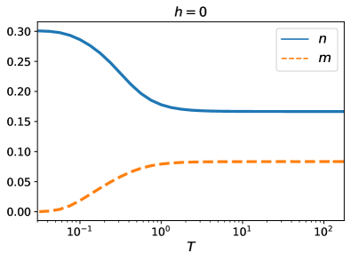
Figure 4: Thermodynamic limit of the densities $n=N/L$, $m=M/L$. The horizontal axis is the temperature $T$.

Let us continue with the $h\neq 0$ case. Let $M_{k}$ be the number of DW with length $k$. Let us the following notations

$$M =M_{2}+M_{3}+M_{4}+\dots$$ (152)

$$yL =L-2N+2-4M_{2}-5M_{3}-6M_{4}-\dots$$ (153)

Furthermore we will use $\mathbf{m}=\{m_{1},m_{2},\dots\}$ with $m_{j}=M_{j}/L$.

The degeneracy of states with these quantum numbers is

$$\frac{(yL+M)!}{(yL)!M_{2}!M_{3}!M_{4}!\dots},$$ (154)

therefore in the thermodynamic limit the DW entropy is

$$S_{DW}(n,\mathbf{m})=(y+m)\log(y+m)-y\log y\\ -m_{2}\log(m_{2})-m_{3}\log m_{3}-m_{4}\log m_{4}-\dots.$$ (155)

The free energy is

$$f[\tilde{\rho},n,\mathbf{m},\alpha]=E[\tilde{\rho},n,m]-TS_{YY}[\tilde{\rho},n,m]\\ -TS_{DW}(n,\mathbf{m})-\alpha\left[(1-n-2m)\int_{0}^{\pi}\tilde{\rho}(p)dp-n\right]\\ +h(n+2m_{2}+3m_{3}+4m_{4}+\dots).$$ (156)

We can see that the $\tilde{\rho}$ and the $\alpha$ dependent parts are the same as before with the same constraint. For the derivatives with respect to $n,m_{k}$ we obtain the following equations

$$\frac{\partial f}{\partial n}: \quad f_{0}(\alpha,n,m)=(1-2m)\alpha$$

$$+2T (1-n-2m)\log\frac{y+m}{y}+(1-n-2m)h,$$ (157)

$$\frac{\partial f}{\partial m_{k}}: \quad f_{0}(\alpha,n,m)=n\alpha$$

$$+\frac{1}{2}T(1-n-2m)\log\frac{(m+y)^{k+1}m_{k}}{y^{k+2}}$$

$$+(1-n-2m)\frac{k}{2}h.$$ (158)

Making proper subtractions we obtain

$$\alpha =\frac{T}{2}\log\frac{m_{2}}{y+m},$$ (159)

$$m_{k+1} =m_{k}\frac{y}{m+y}e^{-\beta h},$$ (160)

therefore

$$m_{k}=m_{2}q^{k-2}$$ (161)

where

$$q=\frac{y}{m+y}e^{-\beta h}.$$ (162)

The number of all DWs can be expressed as

$$m=\sum_{k=2}^{\infty}m_{k}=m_{2}\frac{1}{1-q},$$ (163)

therefore we can expressed all $m_{k}$ and $y$ as

$$m_{k}=m(1-q)q^{k-2},\quad y=1-2n-3m-\frac{1}{1-q}m.$$ (164)

At this point we only have five parameters $(\alpha,n,m,q,y)$ which satisfy the following system of equations

$$\int_{0}^{\pi}\frac{dp}{\pi}\frac{1}{e^{\beta(e(p)-\alpha)}+1}=\frac{n}{1-n-2m},$$ (165)

$$\alpha=\frac{T}{2}\log\frac{m(1-q)}{y+m},$$ (166)

$$\int_{0}^{\pi}\frac{dp}{\pi}\log(1+e^{-\beta(e(p)-\alpha)})$$

$$\qquad\qquad=-\beta\alpha+2\log\frac{y}{m+y}-\beta h,$$ (167)

$$q=\frac{y}{m+y}e^{-\beta h},$$ (168)

$$y=1-2n-3m-\frac{1}{1-q}m.\$$ (169)

Let check the $h\to 0$ limit. In this limit the equations (168,169) simplify as

$$q=\frac{y}{m+y}\quad\longrightarrow\quad 1-q=\frac{m}{m+y},\quad y=\frac{1}{2}(1-2n-4m).$$ (170)

Substituting (166) and (167) we obtain the $h=0$ equations (146),(147) exactly.

Figure 5 shows the numerical results for various $h$. The blue, orange and green curves are the values of $n$, $m$ and $(L/2-S_{z})/L$ w.r.t. the temperature. The graph on the left shows the $h=0$ case which was already plotted on Figure 4, but now we are able to calculate the total spin for the thermal states. We can see that the total spin is zero for every temperature. In the second plot we can see the $h=0.5$ case. The low temperature limit agrees with ground state analysis i.e. the ground state is characterized by a finite particle density $n_{0}\geq 0$. The third picture shows the $h=1.5$ case. Now we can see that the $n$ and the total spin goes to $0$ and $L/2$ for zero temperature as we expected from the ground state analysis. We can also see that the DW density $m$ goes to zero at $T\to 0$ and the $T\to\infty$ limit agrees for all $h$.

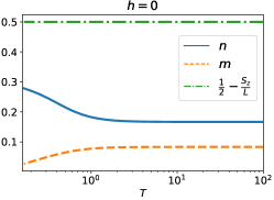
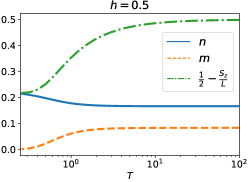
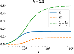
Figure 5: Finite temperature states for $h=0,0.5,1.5$. The orange, blue and green dots show the values of $m$, $n$ and $(L/2-S_{z})/L$ with respect to the temperature.

The equations are simplified again if we use only the variable $x$. Now we define it as

$$x^{2}=e^{-2\beta\alpha}=\frac{y+m}{m(1-q)}.$$ (171)

Since

$$\frac{y}{m+y}=1-\frac{x^{-2}}{1-q},$$ (172)

the equation (167) can be written as

$$\int_{0}^{\pi}\frac{dp}{\pi}\log(x+e^{-\beta e(p)})=2\log F_{h}(x),$$ (173)

where

$$F_{h}(x)=\left(x-\frac{x^{-1}}{1-q}\right)e^{-\beta h/2}.$$ (174)

The variable $q$ can be expressed from (168) which reads as

$$q=\left(1-\frac{x^{-2}}{1-q}\right)e^{-\beta h},$$ (175)

therefore

$$1-q=\frac{x\sinh\left(\frac{\beta h}{2}\right)+\sqrt{1+x^{2}\sinh^{2}\left(\frac{\beta h}{2}\right)}}{x}e^{-\beta h/2}.$$ (176)

Substituting (174) we can obtain that

$$F_{h}(x)=\frac{x^{2}-1}{\sqrt{1+x^{2}\sinh^{2}\left(\tfrac{\beta h}{2}\right)}+x\,\cosh\left(\tfrac{\beta h}{2}\right)}.$$ (177)

The free energy can be also expressed with $x$ as

$$f/T=\beta h-\log\left(x-\frac{x^{-1}}{1-q}\right)=\beta h/2-\log F_{h}(x).$$ (178)

X.2 Thermodynamics in the periodic case

An alternative way is to consider the periodic model and to derive the Thermodynamic Bethe Ansatz (TBA) equations based on the Bethe equations (61). Then we obtain a set of non-linear integral equations, as usually in the TBA framework Takahashi (1999). However, the present case is different from the situation in the XXZ chain, because the scattering kernels are constants. This leads to rather simple equations as opposed to the full XXZ problem.

In the thermodynamic limit we consider again the Bethe root and hole densities $\rho_{n}(p)$, $\rho_{\text{h},n}(p)$, but now with the usual normalization such that in volume $L$ the number of particles/holes for $n$-strings between $p$ and $p+dp$ is $L\rho_{n}(p)dp$ and $L\rho_{n,h}(p)dp$. The densities satisfy

$$\rho_{k}(p)+\rho_{\text{h},k}(p)=\delta_{k,1}\\ +\int_{-\pi}^{\pi}\frac{dp^{\prime}}{4\pi}\left(\rho_{\text{h},k-1}(p^{\prime})+\rho_{\text{h},k+1}(p^{\prime})\right).$$ (179)

This equation can be derived from (61) using the same steps that lead to similar decoupled equations in the XXZ chain for $\Delta>1$, see Takahashi (1999). We see that the total densities are constants, because the r.h.s. of these equations does not carry a $p$-dependence.

In the finite temperature situation we introduce the so-called $Y$-functions as $Y_{n}=\rho_{\text{h},n}/\rho_{n}$. They satisfy the TBA equations

$$\log Y_{n}(p)=\beta\cos(p)\delta_{n,1}\\ +\int_{-\pi}^{\pi}\frac{dp^{\prime}}{4\pi}\log(1+Y_{n-1}(p^{\prime}))(1+Y_{n+1}(p^{\prime})).$$ (180)

It is easy to see that only $Y_{1}(p)$ is a non-trivial function of $p$ all the rest of the $Y$-functions are constants. Written more explicitly, we have the set of equations

$$2\log Y_{1}(p)=2\beta\cos(p)+\log(1+Y_{2}),$$

$$2\log Y_{2}=\int_{-\pi}^{\pi}\frac{dp^{\prime}}{2\pi}\log(1+Y_{1}(p^{\prime}))+\log(1+Y_{3}),$$ (181)

$$Y_{n}^{2}=(1+Y_{n-1})(1+Y_{n+1}),\qquad n\geq 3.$$

The TBA equations can be solved when combining with the asymptotics of $Y$-functions in the large $n$ limit. For $h>0$ the asymptotics is given by

$$\lim_{n\to\infty}\frac{\log Y_{n}}{n}=\beta h.$$ (182)

This implies that for $n\to\infty$, $Y_{n}$ grows exponentially in $n$ as $Y_{n}\sim e^{\beta hn}$. At $h=0$ the asymptotics of the $Y_{n}$ for large $n$ grows polynomially in $n$. Finally, the free energy is given by

$$\frac{F}{L}=\frac{h}{2}-T\int_{-\pi}^{\pi}\frac{dp}{4\pi}\log(1+Y_{1}(p)).$$ (183)

We now discuss the solution of TBA.

Let us denote

$$\beta\alpha=-\frac{1}{2}\log(1+Y_{2}).$$ (184)

The TBA equation can be written as

$$2\log Y_{2}=\int_{-\pi}^{\pi}\frac{dp^{\prime}}{2\pi}\log\left(1+e^{\beta(\cos(p^{\prime})-\alpha)}\right)+\log(1+Y_{3}),$$ (185)

$$Y_{n}^{2}=(1+Y_{n-1})(1+Y_{n+1}),\qquad n\geq 3.$$

We first consider the second equation in (185), which is a second order difference equation. The general solution to this equation is given by

$$Y_{n}=\left(\frac{\sinh([y_{0}+n]a_{0})}{\sinh(a_{0})}\right)^{2}-1,$$ (186)

where $a_{0}$ and $y_{0}$ are two constants. Using the asymptotics (182), we can fix $a_{0}=\beta h/2$. To fix $y_{0}$, we consider (184), which can be written as

$$Y_{2}=e^{-2\beta\alpha}-1=\left(\frac{\sinh([y_{0}+n]\beta h/2)}{\sinh(\beta h/2)}\right)^{2}-1.$$ (187)

From this equation, we can solve $y_{0}$ in terms of $\alpha$. Plugging back to the first equation of (185), we obtain the following equation for the variable $x=e^{-\beta\alpha}$

$$2\log F_{h}(x)=\int_{-\pi}^{\pi}\frac{dp^{\prime}}{2\pi}\log\left(1+x\,e^{\beta\cos(p^{\prime})}\right),$$ (188)

where

$$F_{h}(x)=\frac{x^{2}-1}{\sqrt{1+x^{2}\sinh^{2}\left(\tfrac{\beta h}{2}\right)}+x\,\cosh\left(\tfrac{\beta h}{2}\right)}.$$ (189)

This result is the same as in (177). The TBA equation (188) coincides precisely with the one (173) derived in the previous section. Although (173) is derived by considering open boundary condition, the differences due to boundary conditions are negligible in the thermodynamic limit. Thus we obtained the same TBA equation as expected.

X.3 Thermodynamics in the bond picture

We can also compute the thermodynamics using the Bethe equations (98). A direct application of the TBA framework would lead to two coupled integral equations, corresponding to the two particle species. However, instead of copying the standard formulas of TBA we can also derive the result using a simple reasoning and formulas known from free theories.

Our first argument is that in the direct equations (98) we can assume that the total momentum of the particles and the DW’s is zero; the thermodynamical computations are not sensitive to this assumption. Then we are faced with quantization conditions for two free models, such that the energy is computed only from the particles but it is insensitive to the DW’s. Our strategy is similar as in the previous subsection: we compute the free energy for arbitrary overall densities $n$ and $\tilde{m}$ of the particles and DW’s and afterwards we perform a saddle point analysis. For a direct comparison with the previous formulas we will use $\tilde{m}=2m$, because in the earlier computations $M$ and $m$ denoted the total number and density of the bound states, whereas here $\tilde{m}$ stands for the total density of the DW’s. Each bound state has two domain walls at the two ends, thus the factor of 2 in the relation.

The free energy density will be a sum of the particle and DW contributions:

$$f=f_{p}+f_{DW}.$$ (190)

The computation of the free energy associated to the DW’s is rather simple: as there is no energy, the free energy contribution comes only from the entropy, which is computed easily. We find

$$\beta f_{DW}=-(1-2n-\tilde{m})\log(1-2n-\tilde{m})\\ +(1-2n-2\tilde{m})\log(1-2n-2\tilde{m})+\tilde{m}\log\tilde{m}.$$ (191)

The free energy of the particles at fixed particle number $n$ is computed using a Lagrange multiplier $\alpha$:

$$\beta f_{p}=-(1-n-\tilde{m})\int_{-\pi}^{\pi}\frac{dp}{2\pi}\log(1+e^{-\beta(e(p)-\alpha)})+\beta\alpha n.\\$$ (192)

The value of $\alpha$ is then found from

$$\frac{\partial f}{\partial\alpha}=0$$ (193)

leading to the condition

$$(1-n-\tilde{m})\int_{-\pi}^{\pi}\frac{dp}{2\pi}\frac{1}{1+e^{\beta(e(p)-\alpha)}}=n.$$ (194)

This equation is the same as (145) after the appropriate re-normalization $\tilde{m}=2m$.

XI Solvable Quench Dynamics

The model given by (1) is special because in certain cases the real time dynamics can be solved exactly, leading to exact formulas for the time dependence of local observables. The techniques to be used are completely analogous to those used in Pozsgay (2014); Pozsgay and Eisler (2016), and they were originally developed in Bogoliubov and Malyshev (2011); Bogolyubov and Malyshev (2015); Bogoliubov (2005, 2007); Bogoliubov and Timonen (2011).

Let us focus on quench problems, where we prepare the system in an initial state ${\left|\Psi_{0}\right\rangle}$ and let it evolve with the model Hamiltonian. The simplest problems are those which involve only the particle excitations and not the Domain Walls. Such a situation arises if ${\left|\Psi_{0}\right\rangle}$ has strictly zero overlap with states including DW’s. It is relatively easy to construct such initial states: the only requirement is that in the computational basis there can not be two or more spin excitations on neighbouring positions. For such initial states the overlaps can be computed as a sum over determinants using the exact wave function (19). The simplest cases are those when the initial state is an element of the computational basis, such that the overlaps are single determinants given by (19). We put forward that interesting physics arises in those cases where the bound states are also present; this is discussed in the next Section.

The simplest state with zero overlap with bound states is probably the Néel state where there is a particle excitation at every second site. Using the notation (7) the state is given by

$${\left|\Psi_{0}\right\rangle}={\left|2,4,6,\dots\right\rangle}.$$ (195)

However, in this model the Néel state is actually an eigenstate with eigenvalue 0.

The next simplest case is the period 3 state

$${\left|\Psi^{\prime}_{0}\right\rangle}={\left|3,6,9,\dots\right\rangle}.$$ (196)

Here we have $N$ particles in a volume $L=3N$. This state is not an eigenstate and the overlaps with the Bethe states are given by

$${\langle\Psi^{\prime}_{0}|{\boldsymbol{p}}\rangle}=\det_{jk}e^{ip_{j}(2k+1)}.$$ (197)

This follows from (19) after the substitution $x_{k}=3k$. We will see that the treatment of the quench from this state is very much analogous to the quench problem treated in Section 6 of Pozsgay (2014).

For simplicity we restrict ourselves to the zero momentum sector, therefore we consider the initial state

$${\left|\Psi_{0}\right\rangle}=\frac{1+U+U^{2}}{\sqrt{3}}{\left|\Psi_{0}^{\prime}\right\rangle},$$ (198)

where $U$ is the one-site cyclic shift operator.

In this case the overlaps can be expressed simply as

$$|\langle\Psi_{0}|{\boldsymbol{p}}\rangle|^{2}=\prod_{j<k}|e^{i2p_{j}}-e^{i2p_{k}}|^{-2}.$$ (199)

This overlap will be evaluated in the following.

In the zero momentum sector the Bethe equations are

$$e^{i2Np_{j}}=-1,$$ (200)

where we used $L=3N$ and we assumed an even $N$ for simplicity.

Solutions are given by

$$p_{j}=\frac{\pi(2I_{j}-1)}{2N},\qquad I_{j}=1,2,\dots 2N.$$

The zero momentum Bethe states are given by the subsets

$$\{e^{ip_{j}}\}_{L}\subset\{\omega\}_{2N},\quad\omega_{k}=e^{i\frac{\pi(2k-1)}{2N}},\quad k=1,2,\dots 2N$$

satisfying the constraint $\prod_{j}e^{ip_{j}}=1$. The numbers $\omega_{k}$ can be paired such that

$$\{\omega\}_{2L}=\{(\omega_{k},-\omega_{k})\}_{k=1\dots N}.$$

It follows from formula (199) that the overlap is non-vanishing only if exactly one rapidity is chosen from each pair. Therefore, the states with non-vanishing overlap are given by

$$a_{j}=s_{j}\omega_{j},\quad\text{where}\quad s_{j}=\pm 1,\quad j=1\dots N,$$ (201)

with the constraint that the total momentum is zero. We have

$$1=\prod_{j=1}^{N}e^{ip_{j}}=\prod_{j=1}^{N}(s_{j}\omega_{j})=e^{i\pi N/2}\prod_{j=1}^{N}s_{j}.$$ (202)

We assumed that $N$ is even and the zero momentum constraint implies that there are a total number of $2^{N-1}$ states with non-vanishing overlap.

It can then be seen that the overlaps (199) are all equal and it was shown in Pozsgay (2014) that their value is

$$|\langle\Psi_{0}|{\boldsymbol{p}}\rangle|^{2}=N^{N}.$$ (203)

Our goal is to compute the time evolution of local observables $\mathcal{O}$ using the spectral expansion

$$\left\langle\mathcal{O}(t)\right\rangle=\sum_{{\boldsymbol{p}},{\boldsymbol{k}}}\frac{{\langle\Psi_{0}|{\boldsymbol{p}}\rangle}{\left\langle{\boldsymbol{p}}\right|}\mathcal{O}{\left|{\boldsymbol{k}}\right\rangle}{\langle{\boldsymbol{k}}|\Psi_{0}\rangle}}{{\langle{\boldsymbol{p}}|{\boldsymbol{p}}\rangle}{\langle{\boldsymbol{k}}|{\boldsymbol{k}}\rangle}}e^{-i(E_{\bf k}-E_{\bf p})t}.$$ (204)

We focus on simple local observables, with our main candidates being the operators measuring the emptiness formation probability (EFP). We define the $\ell$-site local operator $\mathbb{E}_{\ell}(x)$ positioned at $x$ as

$$\mathbb{E}_{\ell}(x)=\prod_{j=1}^{\ell}\frac{1+\sigma^{z}_{x-1+j}}{2}.$$ (205)

We also define their space average:

$$\bar{\mathbb{E}}_{\ell}=\frac{1}{L}\sum_{j=1}^{L}\mathbb{E}_{\ell}(j).$$ (206)

The operators $\bar{\mathbb{E}}_{1}$ and $\bar{\mathbb{E}}_{2}$ are conserved, because they are linear combinations of the charges $Q_{1}$, $Q_{2}$ and the identity. Thus the first member of the series with non-trivial time evolution is $\bar{\mathbb{E}}_{3}$.

The matrix element of a single operator $\langle{\boldsymbol{p}}|\mathbb{E}_{\ell}(x)|{\boldsymbol{k}}\rangle$ for arbitrary $\ell$ was computed in Bogoliubov and Malyshev (2011); Bogolyubov and Malyshev (2015)

$$\langle{\boldsymbol{p}}|\mathbb{E}_{\ell}(x)|{\boldsymbol{k}}\rangle=\prod_{j\leq k}\frac{1}{\left(e^{ip_{j}}-e^{ip_{k}}\right)\left(e^{ik_{j}}-e^{ik_{k}}\right)}\det\mathcal{T},$$ (207)

where

$$\mathcal{T}_{jk}=\frac{1-e^{i(k_{j}-p_{k})(L-\ell)}e^{i\left((N-1)(p_{k}-k_{j})\right)}}{e^{ik_{j}}-e^{ip_{k}}}.$$ (208)

The norm of the Bethe states is given by (see Abarenkova and Pronko (2002))

$${\langle{\boldsymbol{p}}|{\boldsymbol{p}}\rangle}=L(L-N)^{N-1}.$$ (209)

The matrix elements of $\mathcal{T}$ can then be rewritten as

$$\mathcal{T}_{jj}=(N-L+\ell-1)e^{-2ik_{j}},\quad p_{j}=k_{k},$$ (210)

$$\mathcal{T}_{jk}=e^{i(\ell-1)(k_{j}+p_{k})}\frac{\sin\left((\ell-1)(k_{j}-p_{k})\right)}{\sin(k_{j}-p_{k})},\quad p_{j}\neq k_{k}.$$ (211)

It is easy to see that for diagonal part of $\mathcal{T}$ the rank is given by the number of coinciding elements in the sets $\boldsymbol{p}$, $\boldsymbol{k}$.

For $\ell=1$ the non-diagonal part is equal to zero, thus the only non-zero contribution to the sum (204) is the case $\boldsymbol{p}=\boldsymbol{k}$ and we obtain trivial time dependence. In the case $\ell=2$ the non-diagonal part has rank 1, thus it is possible to have a non-zero contribution to (204) in a case the diagonal part of matrix $\mathcal{T}$ has the rank at least $N-1$. This happens if there are $N-1$ rapidities $p_{j}$ coinciding with some of rapidities from set $\boldsymbol{k}$. However, due to the $P=0$ condition it is not possible to have a case where the two sets differ only by one rapidity. Thus, for $\ell=2$ case the selection rule for the form factors is again $\boldsymbol{p}=\boldsymbol{k}$ and we have only the static contribution. These findings are consistent with the fact that $\mathbb{E}_{1}$ and $\mathbb{E}_{2}$ are related to the conserved charges $Q_{1}$ and $Q_{2}$.

Finally, for $\ell=3$ the non-diagonal part of $\mathcal{T}$ has rank $2$, thus in order to have a non-zero determinant the rank of the diagonal part should be at least $N-2$. Then there is a time dependence of $\mathbb{E}_{3}(x)$ expectation value if two rapidities are different in the sets $\boldsymbol{p}$ and $\boldsymbol{k}$.

The further computation of dynamics for the case $\ell=3$ is absolutely similar to the one performed in Pozsgay (2014) for the q-boson model. Thus we omit simple details and give here the final result

$$\langle\psi(t)|\mathbb{E}_{3}(x)|\psi(t)\rangle=\frac{1}{6}-\frac{1}{6}\left(\frac{1}{N}\sum_{a}\cos(2\cos(c_{a})t)\right)^{2}\\ -\frac{1}{6}\left|\frac{1}{N}\sum_{a}\sin(2\cos(c_{a})t)e^{ic_{a}}\right|^{2},$$ (212)

where $c_{a}=\pi(2a-1)/(2N)$, $a=1,\dots,N$. In the thermodynamic limit the last expression can be presented as

$$\langle\psi(t)|\mathbb{E}_{3}(x)|\psi(t)\rangle=\frac{1}{6}-\frac{1}{6}\left(\int_{0}^{\pi}\frac{dz}{\pi}\cos(2\cos(z)t)\right)^{2}\\ -\frac{1}{6}\left|\int_{0}^{\pi}\frac{dz}{\pi}\sin(2\cos(z)t)e^{iz}\right|^{2}.$$ (213)

The only difference with the corresponding formula of Pozsgay (2014) (see eq. (6.16) of that work) is the appearance of the extra factor of $1/3$, which can be traced back to the difference in the norm (209) and an overall factor of 3 originating in the definition (198) of the initial state.

The integrals above actually describe the Bessel functions of the first kind, so we can write

$$\langle\psi(t)|\mathbb{E}_{3}(x)|\psi(t)\rangle=\frac{1}{6}\left[1-(J_{0}(2t))^{2}-(J_{1}(2t))^{2}\right].$$ (214)

The asymptotic behaviour for large $t$ is

$$\langle\psi(t)|\mathbb{E}_{3}(x)|\psi(t)\rangle=\frac{1}{6}\left[1-\frac{1}{\pi t}+\mathcal{O}(t^{-2})\right].$$ (215)

We compared (212) to results from exact diagonalization and found complete agreement.

XII Breakdown of the GGE: Persistent oscillations

The large number of degeneracies in the spectrum has an interesting consequence: it can lead to the appearance of persistent oscillations in certain quench problems. Such persistent oscillations can appear in $SU(2)$-symmetric spin chains if a magnetic field is applied, or in more complicated situations Medenjak et al. (2020b) where the degeneracies have a somewhat unexpected algebraic origin Korff (2003); Zadnik et al. (2016); Medenjak et al. (2020b). We will argue below that the present model also supports persistent oscillations. However, in contrast to the solvable quench treated in the previous Section, the treatment of the oscillations is much more involved from a theoretical point of view. At present we do not have an exact derivation of the oscillations, therefore we present their existence as a conjecture, which we support by numerical evidence.

In order to understand the effect we briefly discuss the process of equilibration in integrable models. Let us again assume that we release the model from an initial state ${\left|\Psi_{0}\right\rangle}$ and we investigate the real time dynamics of local observables $\mathcal{O}(t)$. Inserting complete sets of states ${\left|a\right\rangle}$ and ${\left|b\right\rangle}$ in finite volume we get

$$\left\langle\mathcal{O}(t)\right\rangle=\sum_{a,b}{\langle\Psi_{0}|a\rangle}{\left\langle a\right|}\mathcal{O}{\left|b\right\rangle}{\langle b|\Psi_{0}\rangle}e^{-i(E_{b}-E_{a})t}.$$ (216)

In the long time limit (or for long time averages) it is usually assumed that this double sum can be constrained to the diagonal contributions. The idea is that in the generic situation there are not too many degeneracies in the spectrum, the energy levels $E_{a}$ can be considered sufficiently independent, and for large enough times the phases of the off-diagonal contributions average out to zero. This leads to the Diagonal Ensemble (DE)

$$\lim_{T\to\infty}\frac{1}{T}\int_{t=0}^{T}dt\ \left\langle\mathcal{O}(t)\right\rangle=\sum_{a}\left|{\langle\Psi_{0}|a\rangle}\right|^{2}{\left\langle a\right|}\mathcal{O}{\left|a\right\rangle}.$$ (217)

From this expression it is then argued, that the mean values are given by the Generalized Gibbs Ensemble (GGE), which incorporates all conserved charges of the model Essler and Fagotti (2016). The derivation of the GGE is possible if the so-called Generalized Eigenstate Thermalization Hypothesis (GETH) is satisfied. If these assumptions hold then the system will equilibrate and the steady states will not support oscillations in any local observable.

The situation is different in the presence of a large number of degeneracies. Let us now denote by $E_{a}$ the energy eigenvalues, and by a further discrete index $j$ the states ${\left|a,j\right\rangle}$ in the degenerate eigenspaces. Then we have the double sum

$$\lim_{t\to\infty}\left\langle\mathcal{O}(t)\right\rangle=\sum_{a}\sum_{j,k}{\langle\Psi_{0}|a,j\rangle}{\left\langle a,j\right|}\mathcal{O}{\left|a,k\right\rangle}{\langle a,k|\Psi_{0}\rangle}.$$ (218)

In such a situation the long time limit is given not only by the mean values, but rather by a complicated sum involving many off-diagonal matrix elements. Generally we can expect the breakdown of the GGE in such a case. Furthermore, if the degeneracies can be lifted such that the energy differences remain commensurable, then we can observe persistent oscillations.

Let us consider concrete examples in our model. We perform quenches with the Hamiltonian (1), where we set $\mu=0$ for simplicity, but we consider the $h=0$ and $h\neq 0$ cases as well. The larges number of degeneracies appear at $h=0$, while some of these are broken up with fixed differences if $h$ is switched on.

For the initial state our main candidate will be the ferromagnetic state in the $x$ direction, which is given by

$${\left|\Psi_{0}\right\rangle}=\otimes_{j=1}^{L}\frac{1}{\sqrt{2}}\begin{pmatrix}1\\ 1\end{pmatrix}.$$ (219)

This is a good choice because it excites various combinations of particles and domain walls. A key property is that the state breaks the $U(1)$-symmetry of the Hamiltonian, and after the quench the system will be populated by states with different values of the $S^{z}$ global charge.

We choose local operators which also break this $U(1)$-symmetry. We look specifically at

$$D_{k}=\prod_{j=1}^{k}\sigma^{-}_{j}.$$ (220)

These operators change the global $S^{z}$ charge. Therefore their mean values in the DE (or in the GGE) are identically zero.

We conjecture that in our model these observables either tend to a finite mean value (for $h=0$) or they display oscillations (for $h\neq 0$). Both behaviour signals the breakdown of the GGE and the presence of the off-diagonal contributions in (218). The difference between the two behaviours is explained easily: if $h$ is switched on then some of degeneracies are split with fixed amounts according to the global charge $S^{z}$. The operator $\mathcal{O}=D_{k}$ changes $S^{z}$ by a fixed amount, thus every non-zero contribution in the double sum (218) will receive the same phase $e^{ihkt}$.

XII.1 Numerical results

We support our conjecture with numerical evidence, obtained from iTEBD Vidal (2003, 2004) simulations. We used the example code in Pollmann (2016) as a starting point and modified it to our purposes to simulate real-time evolution governed by a four-site Hamiltonian: the state of the system is represented as a four-site translational invariant matrix product state (MPS) Perez-Garcia et al. (2007) with four sets of matrices

$$\begin{split}{\left|\Psi\right\rangle}=\!\!\!\!\!\!\sum_{\dots,j_{k},j_{k+1},j_{k+2},j_{k+3},\dots}&\!\!\!\!\!\!\!\!\!\!\!\!\!\!\!\dots\Lambda_{0}\Gamma_{0}^{j_{k}}\Lambda_{1}\Gamma_{1}^{j_{k+1}}\Lambda_{2}\Gamma_{2}^{j_{k+2}}\Lambda_{3}\Gamma_{3}^{j_{k+3}}\dots\\ &\times{\left|\dots,j_{k},j_{k+1},j_{k+2},j_{k+3},\dots\right\rangle},\end{split}$$ (221)

where both the $\Gamma_{k}^{j}$ and $\Lambda_{k}(k=0,1,2,3)$ are $\chi\times\chi$ matrices, where $\chi$ is the so-called bond dimension. The latter are diagonal and they contain the singular values corresponding to the bi-partition of the system at the given bond. The algorithm uses a first order Suzuki-Trotter decomposition for the time evolution operator. We initialize our system in the state ${\left|\Psi_{0}\right\rangle}$ given by (219) (since it is a simple product state, it can be easily written in a form like (221)) and evolve it with a Trotter step of $\delta t=0.01$. Unfortunately the entanglement entropy grows rapidly in time, which limits the applicability of the method to short times. To check the validity of our results we use several different maximal bond dimensions $\chi_{max}$. The results are shown in Figure 6. The curves confirm the theoretical expectations in the investigated time frame.

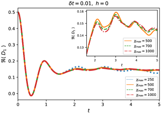
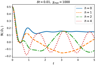
Figure 6: (a) The real part of the expectation value of $D_{1}$ for $h=0$ with different maximal bond dimensions. On the inset the same curves are magnified for $t>1.6$. The data seems to confirm a non-vanishing asymptotic value, but we believe that this evidence is not decisive. The observation of longer times would be desirable, which is not possible with our numerical implementation. (b) The real part of the expectation value of $D_{1}$ for different values of $h$. The maximal bond dimension is $\chi_{max}=1000$, the Trotter time step is $\delta t=0.01$. We observe the predicted oscillation of the expectation value with a frequency directly given by $h$.

XIII Relation with $T\bar{T}$-deformations

Here we point out an interesting relation with the so-called $T\bar{T}$-deformations of QFT’s. Such deformations can be introduced for any QFT, and for the integrable cases it is known that they preserve the integrability of the model Zamolodchikov (2004); Smirnov and Zamolodchikov (2017); Cavaglià et al. (2016). The $T\bar{T}$-deformation modifies the scattering matrix of the model, which is well understood and which we discuss below. Analogues of the $T\bar{T}$-deformation for spin chains were discussed in Pozsgay et al. (2020); Marchetto et al. (2020) pointing out that these transformations are essentially the same as a certain type of long-range deformation studied earlier in the context of the AdS/CFT correspondence Bargheer et al. (2009).

A $T\bar{T}$-like deformation can be introduced for any pair of extensive conserved quantities $Q_{\alpha}$ and $Q_{\beta}$. To first order the deformation consists in modifying the Hamiltonian $H$ of a given model as

$$H^{\prime}=H\\ +\kappa\left(J_{\alpha}(x)q_{\beta}(x)-q_{\alpha}(y)J_{\beta}(x+1)\right)+\mathcal{O}(\kappa^{2}),$$ (222)

where $q_{\alpha}(x)$ are the charge densities and $J_{\alpha}(x)$ are the current operators describing the flow of the charges Pozsgay et al. (2020); Marchetto et al. (2020). Here we gave the formula for the spin chain situation, but an analogous expression gives the corresponding perturbation in the QFT case as well Zamolodchikov (2004); Smirnov and Zamolodchikov (2017); Cavaglià et al. (2016).

If $S(p,k)=e^{i\delta(p,k)}$ is the two-particle scattering matrix of the model, then under the perturbation above it gets deformed as

$$\delta^{\prime}(p,k)=\delta(p,k)\\ +\kappa(h_{\alpha}(p)h_{\beta}(k)-h_{\alpha}(k)h_{\beta}(p))+\mathcal{O}(\kappa^{2})$$ (223)

where $h_{\alpha,\beta}$ are the one-particle eigenvalue functions of the charges $Q_{\alpha}$ and $Q_{\beta}$.

In QFT the actual $T\bar{T}$-deformation corresponds to choosing the energy and the momentum as two charges. An other important case is the so-called hard rod deformation, which corresponds to choosing the particle number and the momentum as the two charges Cardy and Doyon (2020); Jiang (2020). In this case the modification of the $S$-matrix is simply

$$S(p,k)\to S(p,k)\exp\left\{i\kappa(p-k)\right\}.$$ (224)

It is important that the parameter $\kappa$ can be varied continuously, and usually it is assumed to be small compared to some characteristic length scale.

In contrast with the QFT situation it is not possible to construct the $T\bar{T}$ and hard rod deformations on the lattice. On a technical level this happens because on the spin chain there is no momentum operator which would be an extensive local charge. On a physical level this absence comes simply from the discrete structure of the chain.

Quite interestingly, the $S$-matrices that we encountered in this paper have the structure of (224) with an integer $\kappa$ with the undeformed $S$-matrix being $\pm 1$. For example the $S$-matrix factor (15) of the particles in our model is of this form, thus it can be considered a hard rod deformation of the free $S$-matrix of the XX model with $\kappa=-1$. There are other similar examples for this in the literature. For example the $S$-matrix of the phase model (see Pozsgay (2014); Pozsgay and Eisler (2016)) is given by

$$S(p,k)=-e^{i(p-k)}.$$ (225)

This is the hard rod deformation of the XX model $S$-matrix $S(p,k)=-1$ with deformation parameter $\kappa=+1$. Similarly, the $S$-matrix of the constrained XXZ model found in Alcaraz and Bariev (1999); Karnaukhov and Ovchinnikov (2002); Alcaraz and Lazo (2007) can be considered a hard rod deformation of the scattering phases of the XXZ model.

In all of the cases mentioned above there is a non-local transformation which actually connects the deformed model with its undeformed parent model. Then the additional phase in (224) can be interpreted as the additional effect of certain displacements dictated by the non-local transformations. These displacements can be interpreted as the particles having a finite width. Thus we can interpret these models and their non-local transformations as concrete and explicit examples of the hard rod deformation discussed Cardy and Doyon (2020); Jiang (2020).

It is known that in QFT the actual $T\bar{T}$-deformation can be also be interpreted by non-local and field-dependent transformations, and that the particles can be seen as having acquired a (momentum dependent) finite width Caselle et al. (2013); Conti et al. (2019); Cardy and Doyon (2020); Jiang (2020). The examples discussed so far demonstrate such a relation in lattice systems.

Regarding the full spectrum of the present model the situation is somewhat more complicated than in the constrained XXZ model or the phase model. Now the ultimate non-local transformation that maps the interacting model to an (almost) free model concerns the Maassarani-Mathieu chain, which is a spin chain with a different local Hilbert space. Thus we have found a new type of non-local map, which nevertheless belongs to the class of hard rod deformations.

XIV Conclusions

In this work we studied the so-called folded XXZ model which appeared in the earlier works Yang et al. (2020); Zadnik and Fagotti (2021); Zadnik et al. (2021). The main new results of our work are a) the direct connection with the charges of the XXZ model; b) the various forms of the Bethe Ansatz, both with periodic and open boundary conditions; c) the three different descriptions of the thermodynamics; d) the connection with the Maassarani-Mathieu chain; e) the exact solution for a specific quantum quench problem; f) a conjecture for the presence of persistent oscillations, supported by numerical proof; g) making a connection to the $T\bar{T}$ and hard rod deformations, and also to similar models in the literature.

There are a number of interesting open questions.

First of all, it would be interesting to understand the direct algebraic origin of the present model, and how it fits into the Quantum Inverse Scattering Approach Korepin et al. (1993). Our derivation is capable of producing the charges and the eigenstates of the model, nevertheless a direct treatment with the Algebraic Bethe Ansatz is not possible. The reason for this is that the Lax operators which are used in the construction of the transfer matrix of the XXZ model do not survive the $\Delta\to\infty$ limit, or at least this does not happen in a straightforward way. In fact we can prove that the model can not be constructed using the standard way, where the Lax operator is chosen as the $R$-matrix in the fundamental representation: in such cases the charges can be constructed using the boost operator, whereas in our model $Q_{2}$ is not dynamical and a direct application of the boost will not produce the next charge $Q_{3}$; this was discussed in Section IV. Thus the model requires a different Lax operator construction, and a direct $\Delta\to\infty$ of the Lax operators of the XXZ chain will not work.

It would be interesting to consider other models with constant scattering lengths, and hard rod-like $S$-matrix factors, and to formulate the common algebraic origin of these models. So far the known models in this family are the phase model (the $q\to\infty$ limit of the $q$-boson model), the Rule 54 model, and the present one, the folded XXZ model. It would be desirable to develop a unified algebraic framework for such spin chain models. As a particular case of this problem, it would be important to uncover relations between the Rule 54 model and the quantum chains that we treated.

The exact results in these relatively simple models could be used to confirm the predictions of Generalized Hydrodynamics (GHD) in various situations. Such a highly non-trivial check was performed in the recent work Klobas and Bertini (2021) in the case of the Rule 54 model. We believe that the present spin chain and the related models are perfect candidates for such checks: they are quantum models that have genuine interactions, nevertheless they are simple enough that even the spectral sums can be evaluated in certain situations. This presents unique opportunities for exact computations.

Acknowledgments

We are grateful to Maurizio Fagotti, Frank Göhmann, Lorenzo Piroli, Tomaž Prosen, Tibor Rakovszky, Roberto Tateo, Miklós Werner, Lenart Zadnik for useful discussions. In particular we are thankful to Miklós Werner for his help regarding the iTEBD program code and discussions concerning the persistent oscillations.

References

- Caux and Mossel (2011) Jean-Sébastien Caux and Jorn Mossel, “Remarks on the notion of quantum integrability,” J. Stat. Mech. 2011, 02023 (2011), arXiv:1012.3587 [cond-mat.str-el] .
- Essler and Konik (2005) F. Essler and R. M. Konik, “Applications of massive integrable quantum field theories to problems in condensed matter physics,” From Fields to Strings: Circumnavigating Theoretical Physics , 684–830 (2005).
- Guan et al. (2013) Xi-Wen Guan, Murray T. Batchelor, and Chaohong Lee, “Fermi gases in one dimension: From bethe ansatz to experiments,” Rev. Mod. Phys. 85, 1633–1691 (2013).
- Beisert et al. (2012) Niklas Beisert, Changrim Ahn, Luis F. Alday, Zoltan Bajnok, James M. Drummond, et al., “Review of AdS/CFT Integrability: An Overview,” Lett.Math.Phys. 99, 3–32 (2012), arXiv:1012.3982 [hep-th] .
- Calabrese and Cardy (2006) P. Calabrese and J. Cardy, “Time Dependence of Correlation Functions Following a Quantum Quench,” Phys. Rev. Lett. 96, 136801 (2006), cond-mat/0601225 .
- Essler and Fagotti (2016) F. H. L. Essler and M. Fagotti, “Quench dynamics and relaxation in isolated integrable quantum spin chains,” J. Stat. Mech. 6, 064002 (2016), arXiv:1603.06452 [cond-mat.quant-gas] .
- Piroli et al. (2018) L. Piroli, B. Pozsgay, and E. Vernier, “Non-analytic behavior of the Loschmidt echo in XXZ spin chains: exact results,” Nucl. Phys. B 933, 454–481 (2018), arXiv:1803.04380 [cond-mat.stat-mech] .
- Castro-Alvaredo et al. (2016) O. A. Castro-Alvaredo, B. Doyon, and T. Yoshimura, “Emergent Hydrodynamics in Integrable Quantum Systems Out of Equilibrium,” Phys. Rev. X 6, 041065 (2016), arXiv:1605.07331 [cond-mat.stat-mech] .
- Bertini et al. (2016) B. Bertini, M. Collura, J. De Nardis, and M. Fagotti, “Transport in Out-of-Equilibrium XXZ Chains: Exact Profiles of Charges and Currents,” Phys. Rev. Lett. 117, 207201 (2016), arXiv:1605.09790 [cond-mat.stat-mech] .
- Doyon (2017) B. Doyon, “Thermalization and pseudolocality in extended quantum systems,” Comm. Math. Phys. 351, 155–200 (2017), arXiv:1512.03713 [math-ph] .
- Doyon (2020) Benjamin Doyon, “Hydrodynamic projections and the emergence of linearised Euler equations in one-dimensional isolated systems,” arXiv e-prints (2020), arXiv:2011.00611 [math-ph] .
- Borsi et al. (2021) Márton Borsi, Balázs Pozsgay, and Levente Pristyák, “Current operators in integrable models: A review,” arXiv e-prints (2021), arXiv:2103.12160 [cond-mat.stat-mech] .
- Granet and Essler (2021) Etienne Granet and Fabian H. L. Essler, “Systematic strong coupling expansion for out-of-equilibrium dynamics in the Lieb-Liniger model,” arXiv e-prints (2021), arXiv:2102.09987 [cond-mat.stat-mech] .
- Sotiriadis (2020a) Spyros Sotiriadis, “Non-Equilibrium Steady State of the Lieb-Liniger model: exact treatment of the Tonks Girardeau limit,” arXiv e-prints (2020a), arXiv:2007.12683 [cond-mat.stat-mech] .
- Sotiriadis (2020b) Spyros Sotiriadis, “Non-Equilibrium Steady State of the Lieb-Liniger model: multiple-integral representation of the time evolved many-body wave-function,” arXiv e-prints (2020b), arXiv:2010.03553 [cond-mat.stat-mech] .
- Cortés Cubero and Panfil (2020) Axel Cortés Cubero and Miłosz Panfil, “Generalized hydrodynamics regime from the thermodynamic bootstrap program,” SciPost Physics 8 (2020), 10.21468/scipostphys.8.1.004, arXiv:1909.08393 [cond-mat.stat-mech] .
- Sato et al. (2011) J. Sato, B. Aufgebauer, H. Boos, F. Göhmann, A. Klümper, M. Takahashi, and C. Trippe, “Computation of Static Heisenberg-Chain Correlators: Control over Length and Temperature Dependence,” Phys. Rev. Lett. 106, 257201 (2011), arXiv:1105.4447 [cond-mat.str-el] .
- Szecsenyi and Takacs (2012) I. M. Szecsenyi and G. Takacs, “Spectral expansion for finite temperature two-point functions and clustering,” J. Stat. Mech. 1212, P12002 (2012), arXiv:1210.0331 [hep-th] .
- Kozlowski (2015) K. K. Kozlowski, “Asymptotic analysis and quantum integrable models,” ArXiv e-prints (2015), arXiv:1508.06085 [math-ph] .
- Pozsgay and Szécsényi (2018) B. Pozsgay and I. M. Szécsényi, “LeClair-Mussardo series for two-point functions in Integrable QFT,” JHEP 5, 170 (2018), arXiv:1802.05890 [hep-th] .
- Granet and Essler (2020) Etienne Granet and Fabian Essler, “A systematic 1/c-expansion of form factor sums for dynamical correlations in the Lieb-Liniger model,” SciPost Physics 9, 082 (2020), arXiv:2007.15396 [cond-mat.stat-mech] .
- Nagamiya (1940) Takeo Nagamiya, “Statistical mechanics of one-dimensional substances i,” Proc. Phys. Math. Soc. Jpn. 22, 705 (1940).
- Rubin (1955) Robert J. Rubin, “Quantum-mechanical properties of a one-dimensional system composed of hard spheres,” J. Chem. Phys 23, 1183–1186 (1955).
- Sutherland (1971) Bill Sutherland, “Quantum many-body problem in one dimension: Thermodynamics,” J. Math. Phys. 12, 251–256 (1971).
- Boldrighini et al. (1983) C. Boldrighini, R. L. Dobrushin, and Yu. M. Sukhov, “One-dimensional hard rod caricature of hydrodynamics,” J. Stat. Phys. 31, 577–616 (1983).
- Boldrighini and Suhov (1997) C. Boldrighini and Y. M. Suhov, “One-dimensional hard-rod caricature of hydrodynamics: “Navier-Stokes correction” for Local equilibrium initial states,” Comm. Math. Phys. 189, 577–590 (1997).
- Doyon and Spohn (2017) Benjamin Doyon and Herbert Spohn, “Dynamics of hard rods with initial domain wall state,” J. Stat. Mech. 7, 073210 (2017), arXiv:1703.05971 [cond-mat.stat-mech] .
- Cardy and Doyon (2020) John Cardy and Benjamin Doyon, “ deformations and the width of fundamental particles,” arXiv e-prints (2020), arXiv:2010.15733 [hep-th] .
- Jiang (2020) Yunfeng Jiang, “-deformed 1d Bose gas,” arXiv e-prints (2020), arXiv:2011.00637 [hep-th] .
- Hansen et al. (2020) Dennis Hansen, Yunfeng Jiang, and Jiuci Xu, “Geometrizing non-relativistic bilinear deformations,” arXiv e-prints (2020), arXiv:2012.12290 [hep-th] .
- Bobenko et al. (1993) Alexander Bobenko, Martin Bordemann, Charlie Gunn, and Ulrich Pinkall, “On two integrable cellular automata,” Comm. Math. Phys. 158, 127 – 134 (1993).
- Buča et al. (2021) Berislav Buča, Katja Klobas, and Tomaž Prosen, “Rule 54: Exactly solvable model of nonequilibrium statistical mechanics,” arXiv e-prints (2021), arXiv:2103.16543 [cond-mat.stat-mech] .
- Klobas et al. (2019) Katja Klobas, Marko Medenjak, Tomaz Prosen, and Matthieu Vanicat, “Time-dependent matrix product ansatz for interacting reversible dynamics,” Comm. Math. Phys. 371, 651–688 (2019), arXiv:1807.05000 .
- Klobas et al. (2020) Katja Klobas, Bruno Bertini, and Lorenzo Piroli, “Exact thermalization dynamics in the “Rule 54” Quantum Cellular Automaton,” arXiv e-prints (2020), arXiv:2012.12256 [cond-mat.stat-mech] .
- Kos et al. (2018) Pavel Kos, Marko Ljubotina, and Tomaž Prosen, “Many-body quantum chaos: Analytic connection to random matrix theory,” Phys. Rev. X 8, 021062 (2018), arXiv:1712.02665 [nlin.CD] .
- Bertini et al. (2019) Bruno Bertini, Pavel Kos, and Tomaž Prosen, “Exact correlation functions for dual-unitary lattice models in 1+1 dimensions,” Phys. Rev. Lett. 123 (2019), 10.1103/physrevlett.123.210601, arXiv:1904.02140 [cond-mat.stat-mech] .
- Piroli et al. (2020) Lorenzo Piroli, Bruno Bertini, J. Ignacio Cirac, and Tomaž Prosen, “Exact dynamics in dual-unitary quantum circuits,” Phys. Rev. B 101, 094304 (2020), arXiv:1911.11175 [cond-mat.stat-mech] .
- Bogoliubov and Bullough (1992) N M Bogoliubov and R K Bullough, “A q-deformed completely integrable bose gas model,” Journal of Physics A: Mathematical and General 25, 4057 (1992).
- Bogoliubov and Bullough (1992) N. M. Bogoliubov and R. K. Bullough, “Completely integrable model of interacting q-bosons,” Phys. Lett. A 168, 264–269 (1992).
- Bogoliubov et al. (1993) N. M. Bogoliubov, R. K. Bullough, and G. D. Pang, “Exact solution of a q-boson hopping model,” Phys. Rev. B 47, 11495–11498 (1993).
- Bogoliubov et al. (1998) N.M. Bogoliubov, A.G. Izergin, and N.A. Kitanine, “Correlation functions for a strongly correlated boson system,” Nucl. Phys. B 516, 501 – 528 (1998).
- Shigechi and Uchiyama (2005) K. Shigechi and M. Uchiyama, “Boxed skew plane partition and integrable phase model,” J. Phys. A 38, 10287–10306 (2005), cond-mat/0508090 .
- Bogoliubov (2005) N. M. Bogoliubov, “Boxed plane partitions as an exactly solvable boson model,” J. Phys. A 38, 9415–9430 (2005), cond-mat/0503748 .
- Tsilevich (2006) N. V. Tsilevich, “Quantum inverse scattering method for the q-boson model and symmetric functions,” Funct. Anal. Its. Appl. 40, 207–217 (2006), arXiv:math-ph/0510073 [math-ph] .
- Bogoliubov (2007) N. M. Bogoliubov, “Enumeration of plane partitions and the algebraic Bethe anzatz,” Theoretical and Mathematical Physics 150, 165–174 (2007).
- Bogoliubov and Timonen (2011) Nikolay Bogoliubov and Jussi Timonen, “Correlation functions for a strongly coupled boson system and plane partitions,” Philosophical Transactions of the Royal Society of London A: Mathematical, Physical and Engineering Sciences 369, 1319–1333 (2011).
- Pozsgay (2014) B. Pozsgay, “Quantum quenches and generalized Gibbs ensemble in a Bethe Ansatz solvable lattice model of interacting bosons,” J. Stat. Mech. 10, 10045 (2014), arXiv:1407.8344 [cond-mat.stat-mech] .
- Pozsgay and Eisler (2016) B. Pozsgay and V. Eisler, “Real-time dynamics in a strongly interacting bosonic hopping model: Global quenches and mapping to the XX chain,” J. Stat. Mech. 5, 053107 (2016), arXiv:1602.03065 [cond-mat.stat-mech] .
- Medenjak et al. (2020a) Marko Medenjak, Giuseppe Policastro, and Takato Yoshimura, “Thermal transport in -deformed conformal field theories: from integrability to holography,” Phys. Rev. D 103 (2020a), 10.1103/physrevd.103.066012, arXiv:2010.15813 [cond-mat.stat-mech] .
- Yang et al. (2020) Zhi-Cheng Yang, Fangli Liu, Alexey V. Gorshkov, and Thomas Iadecola, “Hilbert-Space Fragmentation from Strict Confinement,” Phys. Rev. Lett. 124, 207602 (2020), arXiv:1912.04300 [cond-mat.str-el] .
- Zadnik and Fagotti (2021) Lenart Zadnik and Maurizio Fagotti, “The Folded Spin-1/2 XXZ Model: I. Diagonalisation, Jamming, and Ground State Properties,” SciPost Phys. Core 4, 10 (2021), arXiv:2009.04995 [cond-mat.stat-mech] .
- Zadnik et al. (2021) Lenart Zadnik, Kemal Bidzhiev, and Maurizio Fagotti, “The Folded Spin-1/2 XXZ Model: II. Thermodynamics and Hydrodynamics with a Minimal Set of Charges,” SciPost Phys. 10, 99 (2021), arXiv:2011.01159 [cond-mat.stat-mech] .
- Fagotti (2014) Maurizio Fagotti, “On conservation laws, relaxation and pre-relaxation after a quantum quench,” J. Stat. Mech. 2014, 03016 (2014), arXiv:1401.1064 [cond-mat.stat-mech] .
- Abarenkova and Pronko (2002) N.I. Abarenkova and A.G. Pronko, “Temperature correlation function in the absolutely anisotropic XXZ Heisenberg Magnet,” Theor. Math. Phys. 131, 690–703 (2002).
- Trippe et al. (2010) Christian Trippe, Frank Göhmann, and Andreas Klümper, “Thermodynamics and short-range correlations of the XXZ chain close to its triple point,” J. Stat. Mech. 2010, 01021 (2010), arXiv:0912.1739 [cond-mat.stat-mech] .
- Alcaraz and Bariev (1999) F. C. Alcaraz and R. Z. Bariev, “An Exactly Solvable Constrained XXZ Chain,” Proceedings for Statistical Physics in the Eve of the 21st Century (Series on Advances in Statistical Mechanics), M. T. Bachelor and L. T. Wille (eds.) vol. 14 Singapore (1999), arXiv:cond-mat/9904042 [cond-mat.stat-mech] .
- Karnaukhov and Ovchinnikov (2002) I. N. Karnaukhov and A. A. Ovchinnikov, “One-dimensional strongly interacting Luttinger liquid of lattice spinless fermions,” EPL (Europhysics Letters) 57, 540–545 (2002), arXiv:cond-mat/0110289 [cond-mat.str-el] .
- Alcaraz and Lazo (2007) Francisco C. Alcaraz and Matheus J. Lazo, “Exactly solvable interacting vertex models,” J. Stat. Mech. 2007, 08008 (2007), arXiv:0706.2178 [cond-mat.stat-mech] .
- Nandkishore and Hermele (2019) Rahul M. Nandkishore and Michael Hermele, “Fractons,” Ann. Rev. Cond. Matt. Phys. 10, 295–313 (2019), arXiv:1803.11196 [cond-mat.str-el] .
- Pretko et al. (2020) Michael Pretko, Xie Chen, and Yizhi You, “Fracton phases of matter,” Int. J. Mod. Phys. A 35, 2030003 (2020), arXiv:2001.01722 [cond-mat.str-el] .
- Note (1) We discovered the model independently, but later we noticed that it was already treated (also independently) in Yang et al. (2020) and in Zadnik and Fagotti (2021); Zadnik et al. (2021).
- Wigner (1955) Eugene P. Wigner, “Lower limit for the energy derivative of the scattering phase shift,” Phys. Rev. 98, 145–147 (1955).
- Tetelman (55) M. G. Tetelman, “Lorentz group for two-dimensional integrable lattice systems,” Sov. Phys. JETP 1981, 306 (55).
- Thacker (1986) H. B. Thacker, “Corner transfer matrices and Lorentz invariance on a lattice,” Physica D Nonlinear Phenomena 18, 348–359 (1986).
- Grabowski and Mathieu (1995) M.P. Grabowski and P. Mathieu, “Structure of the conservation laws in integrable spin chains with short range interactions,” Annals Phys. 243, 299–371 (1995), arXiv:hep-th/9411045 [hep-th] .
- Grabowski and Mathieu (1994) Marek P. Grabowski and Pierre Mathieu, “Quantum integrals of motion for the Heisenberg spin chain,” Mod.Phys.Lett. A9, 2197–2206 (1994), arXiv:hep-th/9403149 [hep-th] .
- Nozawa and Fukai (2020) Yuji Nozawa and Kouhei Fukai, “Explicit Construction of Local Conserved Quantities in the XYZ Spin-1/2 Chain,” Phys. Rev. Lett. 125, 090602 (2020), arXiv:2003.02856 [cond-mat.stat-mech] .
- Nienhuis and Huijgen (2021) Bernard Nienhuis and Onno Huijgen, “All local conserved quantities of the XXZ model,” arXiv e-prints (2021), arXiv:2104.01851 [math-ph] .
- Kulish (1976) P. P. Kulish, “Factorization of the classical and the quantum s matrix and conservation laws,” Theor Math Phys 26, 132 (1976).
- Takahashi (1999) Minoru Takahashi, Thermodynamics of One-Dimensional Solvable Models (Cambridge University Press, 1999).
- Pozsgay (2013) B. Pozsgay, “The generalized gibbs ensemble for heisenberg spin chains,” J. Stat. Mech. 2013, 3 (2013), arXiv:1304.5374 [cond-mat.stat-mech] .
- Bogoliubov and Malyshev (2011) N. M. Bogoliubov and C. L. Malyshev, “Ising limit of a Heisenberg XXZ magnet and some temperature correlation functions,” Theor. Math. Phys. 169, 1517–1529 (2011), arXiv:1106.5455 [cond-mat.stat-mech] .
- Bogolyubov and Malyshev (2015) N. M. Bogolyubov and C. L. Malyshev, “Integrable models and combinatorics,” Russ. Math. Surv. 70, 789–856 (2015).
- Mossel and Caux (2010) J. Mossel and J.-S. Caux, “Relaxation dynamics in the gapped XXZ spin-1/2 chain,” New Journal of Physics 12, 055028 (2010), arXiv:1002.3988 [cond-mat.str-el] .
- Sklyanin (1988) E K Sklyanin, “Boundary conditions for integrable quantum systems,” J. Phys. A 21, 2375 (1988).
- Batchelor et al. (1995) M. T. Batchelor, R. J. Baxter, M. J. O’Rourke, and C. M. Yung, “Exact solution and interfacial tension of the six-vertex model with anti-periodic boundary conditions,” J. Phys. A 28, 2759–2770 (1995), arXiv:hep-th/9502040 [hep-th] .
- Yung and Batchelor (1995) C. M. Yung and M. T. Batchelor, “Exact solution for the spin-s XXZ quantum chain with non-diagonal twists,” Nucl. Phys. B 446, 461–484 (1995), arXiv:hep-th/9502041 [hep-th] .
- Maassarani and Mathieu (1998) Z. Maassarani and P. Mathieu, “The su(N) XX model,” Nucl. Phys. B 517, 395–408 (1998), arXiv:cond-mat/9709163 [cond-mat.stat-mech] .
- Bariev (1991) R Z Bariev, “Integrable spin chain with two- and three-particle interactions,” J. Phys. A: Math. Gen. 24, L549–L553 (1991).
- Göhmann and Murakami (1998) Frank Göhmann and Shuichi Murakami, “Fermionic representations of integrable lattice systems,” J. Phys. A 31, 7729–7749 (1998), arXiv:cond-mat/9805129 [cond-mat] .
- Essler et al. (2005) Fabian H. L. Essler, Holger Frahm, Frank Göhmann, Andreas Klümper, and Vladimir E. Korepin, The One-Dimensional Hubbard Model (Cambridge University Press, Cambridge, 2005).
- Sala et al. (2020) Pablo Sala, Tibor Rakovszky, Ruben Verresen, Michael Knap, and Frank Pollmann, “Ergodicity Breaking Arising from Hilbert Space Fragmentation in Dipole-Conserving Hamiltonians,” Phys. Rev. X 10, 011047 (2020), arXiv:1904.04266 [cond-mat.str-el] .
- Khemani et al. (2020) Vedika Khemani, Michael Hermele, and Rahul Nandkishore, “Localization from Hilbert space shattering: From theory to physical realizations,” Phys. Rev. B. 101, 174204 (2020), arXiv:1910.01137 [cond-mat.stat-mech] .
- Medenjak et al. (2020b) Marko Medenjak, Berislav Buča, and Dieter Jaksch, “Isolated Heisenberg magnet as a quantum time crystal,” Phys. Rev. B 102, 041117 (2020b), arXiv:1905.08266 [cond-mat.stat-mech] .
- Korff (2003) Christian Korff, “Auxiliary matrices for the six-vertex model at qN = 1 and a geometric interpretation of its symmetries,” J. Phys. A 36, 5229–5266 (2003), arXiv:math-ph/0302002 [math-ph] .
- Zadnik et al. (2016) Lenart Zadnik, Marko Medenjak, and Tomaž Prosen, “Quasilocal conservation laws from semicyclic irreducible representations of Uq (sl2) in XXZ spin-1/2 chains,” Nucl. Phys. B 902, 339–353 (2016), arXiv:1510.08302 [math-ph] .
- Vidal (2003) G. Vidal, “Efficient Classical Simulation of Slightly Entangled Quantum Computations,” Phys. Rev. Lett. 91, 147902 (2003), quant-ph/0301063 .
- Vidal (2004) G. Vidal, “Efficient Simulation of One-Dimensional Quantum Many-Body Systems,” Phys. Rev. Lett. 93, 040502 (2004), quant-ph/0310089 .
- Pollmann (2016) Frank Pollmann, “Efficient numerical simulations using matrix-product states,” (2016).
- Perez-Garcia et al. (2007) D. Perez-Garcia, F. Verstraete, M. M. Wolf, and J. I. Cirac, “Matrix Product State Representations,” Quantum Info. Comput. 7, 401–430 (2007), quant-ph/0608197 .
- Zamolodchikov (2004) Alexander B. Zamolodchikov, “Expectation value of composite field in two-dimensional quantum field theory,” arxiv e-prints (2004), arXiv:hep-th/0401146 [hep-th] .
- Smirnov and Zamolodchikov (2017) F. A. Smirnov and A. B. Zamolodchikov, “On space of integrable quantum field theories,” Nucl. Phys. B 915, 363–383 (2017), arXiv:1608.05499 [hep-th] .
- Cavaglià et al. (2016) Andrea Cavaglià, Stefano Negro, István M. Szécsényi, and Roberto Tateo, “-deformed 2D Quantum Field Theories,” JHEP 10, 112 (2016), arXiv:1608.05534 [hep-th] .
- Pozsgay et al. (2020) Balázs Pozsgay, Yunfeng Jiang, and Gábor Takács, “-deformation and long range spin chains,” JHEP 03, 092 (2020), arXiv:1911.11118 [hep-th] .
- Marchetto et al. (2020) Enrico Marchetto, Alessandro Sfondrini, and Zhou Yang, “ deformations and integrable spin chains,” Phys. Rev. Lett. 124, 100601 (2020), arXiv:1911.12315 [hep-th] .
- Bargheer et al. (2009) Till Bargheer, Niklas Beisert, and Florian Loebbert, “Long-range deformations for integrable spin chains,” J. Phys. A 42, 285205 (2009), arXiv:0902.0956 [hep-th] .
- Caselle et al. (2013) Michele Caselle, Davide Fioravanti, Ferdinando Gliozzi, and Roberto Tateo, “Quantisation of the effective string with TBA,” JHEP 07, 071 (2013), arXiv:1305.1278 [hep-th] .
- Conti et al. (2019) Riccardo Conti, Stefano Negro, and Roberto Tateo, “The perturbation and its geometric interpretation,” JHEP 02, 085 (2019), arXiv:1809.09593 [hep-th] .
- Korepin et al. (1993) V.E. Korepin, N.M. Bogoliubov, and A.G. Izergin, Quantum inverse scattering method and correlation functions (Cambridge University Press, 1993).
- Klobas and Bertini (2021) Katja Klobas and Bruno Bertini, “Exact relaxation to Gibbs and non-equilibrium steady states in the quantum cellular automaton Rule 54,” arXiv e-prints (2021), arXiv:2104.04511 [cond-mat.stat-mech] .