Near-unit efficiency of chiral state conversion via hybrid-Liouvillian dynamics

Abstract

Following the evolution under a non-Hermitian Hamiltonian (nHH) involves significant probability loss. This makes various nHH effects impractical in the quantum realm. In contrast, Lindbladian evolution conserves probability, facilitating observation and application of exotic effects characteristic of open quantum systems. Here we are concerned with the effect of chiral state conversion: encircling an exceptional point, multiple system states are converted into a single system eigenmode. While for nHH the possible converted-into eigenmodes are pure states, for Lindbladians these are typically mixed states. We consider hybrid-Liouvillian evolution, which interpolates between a Lindbladian and a nHH and enables combining the best of the two worlds. We design adiabatic evolution protocols that give rise to chiral state conversion with pure final states, no probability loss, and high fidelity. Furthermore, extending beyond continuous adiabatic evolution, we design a protocol that facilitates conversion to pure states with fidelity 1 and, at the same time, no probability loss. Employing recently developed experimental techniques, our proposal can be implemented with superconducting qubit platforms.

Introduction.—Over the past few years, exceptional points (EPs) of non-Hermitian Hamiltonians (Kato, 1995; Berry, 2004; Heiss, 2012; Ashida et al., 2020) have become an object of intense study in a number of distinct contexts. From rather abstract studies involving $\mathcal{PT}$-symmetric nHHs (Bender and Boettcher, 1998; Bender, 2007; Christodoulidess and Yang, 2018; Bender, 2019), adiabatic nHH evolution (Mailybaev et al., 2005; Berry and Uzdin, 2011; Milburn et al., 2015; Doppler et al., 2016; Hassan et al., 2017; Pick et al., 2017; Zhang et al., 2018a; Zhong et al., 2018; Miri and Alù, 2019; Liu et al., 2021), topological manifestations (Wang et al., 2009; Lefebvre et al., 2009; Uzdin et al., 2011; Rechtsman et al., 2013; Chang et al., 2014; El-Ganainy et al., 2018), exotic band structures (Zhen et al., 2015), and properties of non-equilibrium phase transitions (Altland et al., 2020; Soriente et al., 2021) to more practically-oriented proposals of loss-induced transparency and lasing (Guo et al., 2009; Peng et al., 2014; Jing et al., 2014; Brandstetter et al., 2014; Miao et al., 2016; Zhang et al., 2018b), on-demand directional emission (Kim et al., 2014; Wiersig, 2014; Peng et al., 2016; Li et al., 2020), optimal energy transfer (Xu et al., 2016; Assawaworrarit et al., 2017), and enhanced sensing (Chen et al., 2017; Hodaei et al., 2017; Zhang et al., 2019).

One of the most striking effects emerging in the vicinity of an EP is chiral state conversion (Mailybaev et al., 2005; Berry and Uzdin, 2011; Milburn et al., 2015; Doppler et al., 2016; Hassan et al., 2017; Pick et al., 2017; Zhang et al., 2018a; Zhong et al., 2018; Miri and Alù, 2019): Under adiabatic evolution of the system along a trajectory in the parameter space such that an EP is encircled, all possible initial states of the system are converted to one final state. The final state corresponds to one of the system’s eigenmodes. The directionality of the winding around the EP (the chirality) determines which eigenmode it is. A major hindrance in employing this chiral effect for practical purposes or incorporating it in more complex manipulation protocols, are the significant losses incurred under nHH evolution. These may be acceptable in classical applications; in the quantum context, any loss of probability is highly detrimental.

While classical lossy systems are often naturally described in terms of a nHH, open quantum systems only allow for such a description in the presence of postselection, based on monitoring of the environment (Naghiloo et al., 2019; Chen et al., 2021). In the presence of a non-monitored Markovian environment, quantum system evolution is described by the Lindblad master equation (Carmichael, 1999; Gardiner and Zoller, 2004; Haroche and Raimond, 2006; Breuer and Petruccione, 2007). The physics of EPs of Lindbladian superoperators is attracting much attention (Hatano, 2019; Pick et al., 2019; Minganti et al., 2019, 2020; Arkhipov et al., 2020a, b; Gunderson et al., 2020; Kumar et al., 2021; Gulácsi and Dóra, 2021; Khandelwal et al., 2021), in particular, in the context of optimal state preparation and stabilization (Pick et al., 2019; Kumar et al., 2021; Khandelwal et al., 2021). Lindbladian evolution conserves the total probability, eliminating losses and, naively, opening the way to efficient chiral state conversion in the quantum realm. However, generically the eigenmodes involved (i.e., the potential conversion results) do not correspond to pure states, limiting the applicability of such protocols (Pick et al., 2019).

Here we investigate chiral state conversion in a system featuring a controllable degree of postselection, cf. Fig. 1(a). The dynamics is described within the hybrid-Liouvillian (hL) formalism (Minganti et al., 2020). Depending on the postselection parameter, $q$, the hL interpolates between nHH ($q=0$) and Lindbladian ($q=1$) dynamics. We show that the EPs of the hL form a rich structure within the parameter space extended by $q$. This structure continuously connects the EPs of the Lindbladian at $q=1$ to those of the corresponding nHH at $q=0$, opening the way for chiral state conversion with the degree of postselection being varied during the protocol. This way the best of the two worlds can be combined: low losses, inherent to $q\approx 1$ evolution, and pure state eigenmodes, inherent to $q=0$.

Below we show that varying $q$ during the evolution alongside the other parameters significantly reduces the probability loss, while the mode conversion fidelity (that quantifies the accuracy of mode conversion) remains almost unchanged. We note, though, that even with the protocol where $q$ is varied during the adiabatic evolution, the two desired goals: (i) perfect values of unit fidelity and (ii) no loss due to postselection, are unattainable simultaneously. To achieve these two goals together, we further employ a “hopping strategy”, developed recently in the context of nHH dynamics (Li et al., 2020): we replace parts of the adiabatic encircling trajectory by abrupt hops. We demonstrate that combining the hopping strategy with a controlled postselection parameter, $q$, facilitates achieving both goals mentioned above, cf. Fig. 3.

Model.—We study a single qubit subject to a Hamiltonian evolution and spontaneous relaxation processes, cf. Fig. 1(a). When the qubit is in an excited state, $\left|\uparrow\right\rangle$, it can relax to the ground state, $\left|\downarrow\right\rangle$, by emitting a photon. Whenever a photon is emitted, the experimental run is either interrupted and discarded from the statistics (probability $1-q$) or is allowed to proceed (probability $q$) depending on which detector clicks (Imp, ). The resulting evolution of the qubit density matrix is described by the following Liouville equation:

$$\frac{d\rho}{dt}=\mathcal{L}_{q}[\rho]=-i[H,\rho]-\frac{\gamma}{2}\left(\{L^{\dagger}L,\rho\}-2qL\rho L^{\dagger}\right),$$ (1)

with the Hamiltonian

$$H=\frac{\omega}{2}\left(\sin\theta\,\sigma_{x}+\cos\theta\,\sigma_{z}\right)\equiv\frac{\omega_{x}}{2}\sigma_{x}+\frac{\omega_{z}}{2}\sigma_{z},$$ (2)

the Lindblad jump operator $L=\left|\downarrow\right\rangle\left\langle\uparrow\right|$, and the relaxation rate $\gamma$. Note that Eq. (1) does not preserve the probability (density matrix trace) unless $q=1$, so it is not a proper Liouvillian evolution (hence the name of hybrid-Liouvillian (Minganti et al., 2020)).

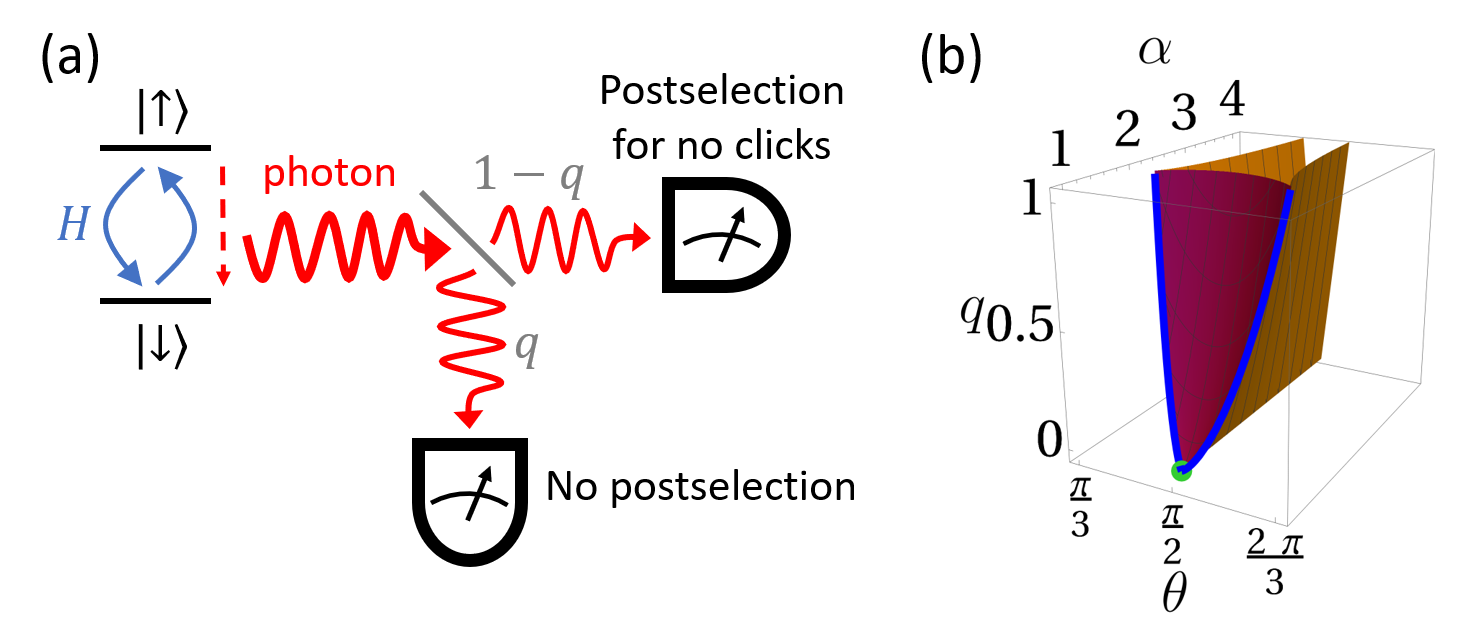
Figure 1: (a)—The setup under consideration. A qubit is subject to a Hamiltonian evolution and relaxation processes. Whenever a relaxation event takes place, the experimental run is discarded with a prescribed probability, $1-q$. (b)—The manifold of EPs of the hybrid-Liouvillian $\mathcal{L}_{q}$, cf. Eqs. (1-4), in the parameter space of $\theta$ (specifying the Hamiltonian), $q$ and $\alpha=\gamma/2\omega$ (determining the relative strength of the Hamiltonian and relaxation). The green point ($\alpha=1,\leavevmode\nobreak\ \theta=\frac{\pi}{2},\leavevmode\nobreak\ q=0$) corresponds to a 4th order degeneracy (featuring, however, only a 3rd order EP) — the hybrid-Liouvillian counterpart of the EP of the nHH $\tilde{H}$, cf. Eq. (3). At $q>0$ the degenerate manifold splits into two lines (blue) of 3rd order EPs connected by a surface of 2nd order EPs (purple). Two more surfaces of 2nd order EPs (orange) are bounded by the blue lines and continue up to $\alpha\rightarrow\infty$; their intersection at $q=0$ forms a line of 2nd order degeneracies, which are not EPs.

In the absence of postselection, $q=1$, one recovers the standard Lindblad equation (Carmichael, 1999; Gardiner and Zoller, 2004; Haroche and Raimond, 2006; Breuer and Petruccione, 2007). In the case of perfect postselection, $q=0$, the system evolution can be described in terms of a non-Hermitian Hamiltonian $\tilde{H}$:

$$\frac{d\rho}{dt}=-i\left(\tilde{H}\cdot\rho-\rho\cdot\tilde{H}^{\dagger}\right),\quad\tilde{H}=H-i\frac{\gamma}{2}\,L^{\dagger}L.$$ (3)

We consider the range of parameters to be $\omega\geq 0$ and $\theta\in[0,\pi]$. We further define a dimensionless parameter $\alpha=\frac{\gamma}{2\omega}\geq 0$.

Hybrid-Liouvillian Exceptional Points.—To model the chiral behavior marking the hL dynamics of encircling EPs in parameter space, first we need to investigate the EPs of the superoperator $\mathcal{L}_{q}$ defined in Eq. (1). The present, rather technical section, summarizes the steps taken to obtain Fig. 1(b). For that purpose, it is convenient to write the matrix representation of the superoperator:

$$\mathcal{L}_{q}=\left(\begin{array}[]{cccc}-\gamma&i\frac{\omega_{x}}{2}&-i\frac{\omega_{x}}{2}&0\\ i\frac{\omega_{x}}{2}&-\frac{\gamma}{2}-i\omega_{z}&0&-i\frac{\omega_{x}}{2}\\ -i\frac{\omega_{x}}{2}&0&-\frac{\gamma}{2}+i\omega_{z}&i\frac{\omega_{x}}{2}\\ \gamma q&-i\frac{\omega_{x}}{2}&i\frac{\omega_{x}}{2}&0\end{array}\right)$$ (4)

in the basis $\{\rho_{\uparrow\uparrow},\rho_{\uparrow\downarrow},\rho_{\downarrow\uparrow},\rho_{\downarrow\downarrow}\}$. The superoperator’s eigenvalues $\{\lambda\}$ correspond to zeros of the characteristic polynomial $\mathcal{C}_{q}(\lambda)=\text{Det}(\mathcal{L}_{q}-\lambda\mathbb{\,I})$, where $\mathbb{I}$ is the identity matrix. An $n$th order EP corresponds to an $n$th order degeneracy where $n$ eigenvectors coalesce into a single eigenvector. We first look for the set of $n$th order degeneracies by requiring $\mathcal{C}_{q}(\lambda_{d})=...=\mathcal{C}_{q}^{(n-1)}(\lambda_{d})=0$, where $\mathcal{C}_{q}^{(k)}(\lambda)$ denotes the $k$th derivative of the characteristic polynomial. We then check the number of linearly independent eigenvectors corresponding to this $\lambda_{d}$ in order to separate EPs from trivial degeneracies.

Figure 1(b) shows the resulting locations of the EPs and non-EP degeneracies in the space of protocol parameters $(\alpha,\theta,q)$ (Sup, ). We find a 4th order degeneracy located at $(1,\pi/2,0)$ (green point). At $q=0$, the system can be described by a nHH, $\tilde{H}$ in Eq. (3), which has a well-studied (Milburn et al., 2015; Doppler et al., 2016; Hassan et al., 2017; Zhang et al., 2018a; Miri and Alù, 2019; Li et al., 2020) 2nd order EP at $\alpha=1$, $\theta=\pi/2$. In the language of hL, this nHH EP becomes a 4th order degeneracy. However, it is only a 3rd order EP: only three eigenvectors of hL coalesce while the fourth remains separate. At $(\alpha>1,\pi/2,0)$, we also find a line of 2nd order degeneracies of $\mathcal{L}_{q}$, which are not EPs.

As soon as $q\neq 0$ we find a more involved spectrum of EPs. At each $q>0$, we find two EPs of 3rd order and three lines of 2nd order EPs. Taken for all $q\in(0;1]$ the structure becomes two lines of 3rd order EPs and three surfaces of 2nd order EPs, cf. Fig. 1(b).

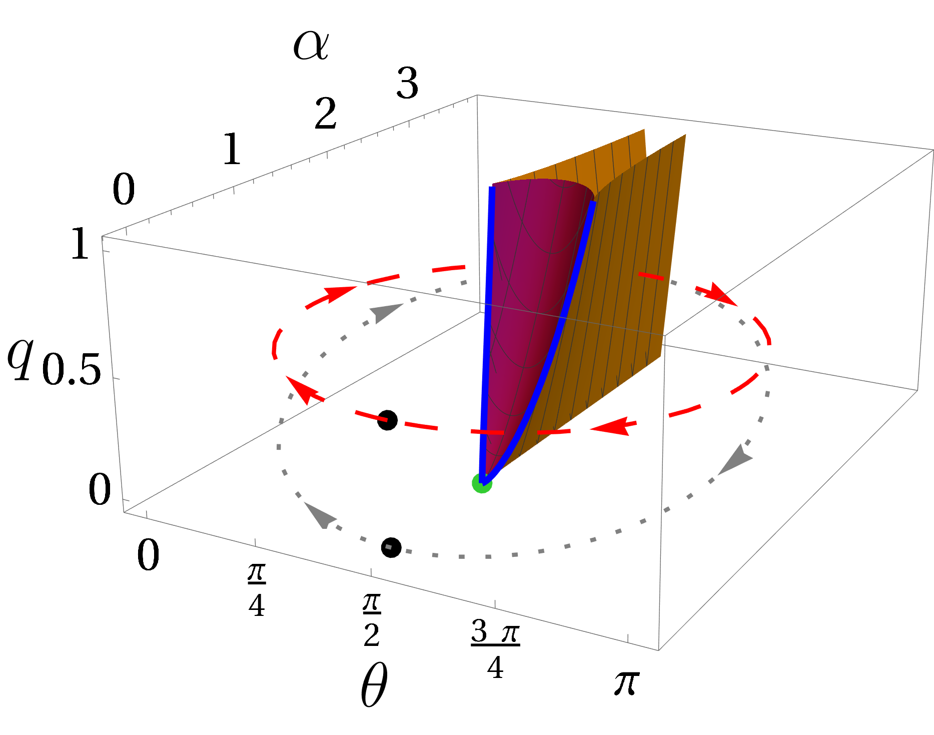
Figure 2: Trajectories encircling the central part of the EP structure. The tilted trajectories ($q\neq\text{const}$, dotted gray), defined in Eq. (5), all start at the same point $(\alpha,\theta,q)=(0,\pi/2,0)$, but can approach different values of $q_{0}$ in the middle of the closed trajectory. Flat trajectories (dashed red), defined in Eq. (6), correspond to $q=q_{0}$ plane. The black dots represent the starting (and end) point of the corresponding trajectories.

X-adiabatic encircling of the EP structure.—We are now in a position to discuss chiral state conversion in the system. We start with some abstract arguments for why it could be expected and what the caveats are. We then resort to a numerical investigation and discuss its results confirming and quantifying the expected behavior.

Consider the EP manifold in the $(\alpha,\theta,q)$ space, cf. Fig. 1(b). Let us for a moment ignore the fact that the EP manifold extends to $\alpha\rightarrow\infty$ and pretend that one can encircle it. The chirality of chiral state conversion originates in the switching of the system eigenmodes as one goes around an exceptional point (Zhong et al., 2018). The switching itself stems from the spectrum non-analiticity at the EP. Since the EP manifold is continuous as a function of $q$, the effective non-analiticity of the entire EP manifold should be the same at any given $q$. This implies that the switching of the respective eigenmodes at different $q$ obeys the same rules. Therefore, one expects the same chiral state conversion behavior at all $q$. Note, however, that the eigenmodes of the hL are $q$-dependent, i.e., the final state may depend on the value of $q$ at the beginning/end of the trajectory.

Recall now that the structure extends to $\alpha\rightarrow\infty$, so that encircling the entire structure is impossible. It follows that it is impossible to encircle even part of the structure in a completely adiabatic way. For example, trying to encircle the lines of 3rd order EPs one must cross the surfaces of 2nd order EPs, cf. Fig. 2. On that sub-manifold some of the eigenvalues coincide making it impossible to satisfy the adiabaticity condition (Adi, ). We call such evolution x-adiabatic, i.e. adiabatic everywhere except for a few points along the trajectory.

In order to investigate chiral state conversion under x-adiabatic evolution, we perform a numerical investigation for two families of closed trajectories, cf. Fig. 2. The first family comprises trajectories that start and end in the $q=0$ plane, with the postselection rate varied along the trajectory. The second family comprises trajectories with a fixed $q$, i.e. the postselection rate remains constant along the trajectory. In reference to their shape, we denote the first family tilted and the second one flat. The tilted trajectories start at $(0,\pi/2,0)$, then reach $(\alpha_{0},\pi/2,q_{0})$ at the mid-point, and finally return back to the initial point:

$$\alpha_{\textrm{tilted}}(t)=3\sin^{2}\frac{\pi t}{T},\quad q_{\textrm{tilted}}(t)=q_{0}\sin^{2}\frac{\pi t}{T},$$ (5)

$$\theta_{\textrm{tilted}}(t)=\frac{\pi}{2}-\frac{3}{2}\sin\frac{2\pi\chi t}{T},$$

where the evolution takes place within the time interval $t\in[0,T]$, and $\chi=\pm 1$ corresponds to different winding chiralities. The flat trajectories start/end at $(0,\pi/2,q_{0})$ and remain in $q=q_{0}$ plane at all intermediate times:

$$\alpha_{\textrm{flat}}(t)=3\sin^{2}\frac{\pi t}{T},\quad q_{\textrm{flat}}(t)=q_{0},$$ (6)

$$\theta_{\textrm{flat}}(t)=\frac{\pi}{2}-\frac{3}{2}\sin\frac{2\pi\chi t}{T}.$$

Consider first the tilted trajectories. The $q_{0}=0$ trajectory can be equivalently described by a nHH $\tilde{H}$, cf. Eq. (3). This problem is well studied (Milburn et al., 2015; Doppler et al., 2016; Hassan et al., 2017; Zhang et al., 2018a; Miri and Alù, 2019; Li et al., 2020). At the initial and final point, the system experiences only the Hamiltonian $H$, cf. Eq. (2), whose eigenstates are $\left|\pm\right\rangle=(\left|\uparrow\right\rangle\pm\left|\downarrow\right\rangle)/\sqrt{2}$. Adiabatically ($T\rightarrow\infty$) following this trajectory at $q_{0}=0$ in the clockwise direction ($\chi=+1$) leads to a conversion of any initial system state to $\rho_{\chi=+1}=\left|+\right\rangle\left\langle+\right|$. Following the trajectory in the opposite direction ($\chi=-1$) converts any initial state to $\rho_{\chi=-1}=\left|-\right\rangle\left\langle-\right|$. Note that in the hL language this trajectory is x-adiabatic (the trajectory crosses the line of 2nd order degeneracies at $(\alpha>1,\theta=\pi/2,q=0)$). Nevertheless, the outcome of the evolution should coincide with the prediction of the nHH formalism.

For $q_{0}\neq 0,$ we observe the same conversion behavior: any initial state is converted into $\rho_{\chi}$ corresponding to the respective direction $\chi$, as quantified by the fidelity $F=\mathrm{Tr}\,\rho(T)\rho_{\chi}$, cf. Fig. 3(a). Note that the conversion fidelity for tilted trajectories is almost independent of the value of $q_{0}$.

The protocol, however, comes with a significant probability loss. The dependence of the probability $P=\mathrm{Tr}\,\rho(T)$ of carrying out the experiment to the end, without having to discard it due to postselection, is presented in Fig. 3(b). As expected, $P$ increases with $q_{0}$: for higher $q_{0}$ less postselection is applied throughout the trajectory. Yet, even with $q_{0}=1$, $P\approx 10^{-2}$, far from being practically useful.

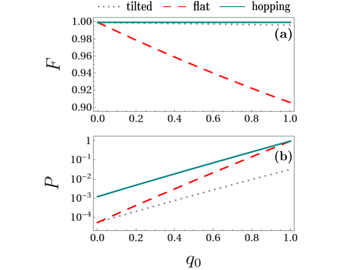
Figure 3: State conversion fidelity $F=\mathrm{Tr}\,\rho(T)\rho_{\chi}$ and postselection probability $P=\mathrm{Tr}\,\rho(T)$ for tilted (dotted gray, Eq. (5)), flat (dashed red, Eq. (6)), and hopping (solid teal, Eqs. (7-9)) trajectory as a function of the postselection parameter $q_{0}$. For all trajectories we took a maximally mixed initial state, $\rho_{i}=\frac{1}{2}\left|+\right\rangle\left\langle+\right|+\frac{1}{2}\left|-\right\rangle\left\langle-\right|$, $\omega=1\leavevmode\nobreak\ ns^{-1}$ for the Liouvillian $\mathcal{L}_{q}$ (cf. Eqs. (1–4)) and a total evolution time $T=100\leavevmode\nobreak\ ns$. For the hopping trajectory, $T_{1}=0.2T$, $T_{2}=0.6T$, $\alpha_{\mathrm{i}}=10^{-5}$, and $\alpha_{\mathrm{ii}}=10$. The values of $F$ and $P$ for clockwise ($\chi=+1$) and counterclockwise ($\chi=-1$) trajectories coincide, hence only three curves are shown.

For flat trajectories, the postselection probability can be much higher, cf. Fig. 3(b). In particular, for $q_{0}=1$ there is no probability loss (as no postselection is applied). However, this comes at the price of a significant fidelity loss. Let us briefly explain the reasons for the latter. The initial/final point of the flat trajectory is $(\alpha,\theta,q)=(0,\pi/2,q_{0})$, so that $\gamma=2\omega\alpha=0$. Therefore, the system eigenmodes at the initial/final point of the trajectory are determined by the same parameters of $H$ in Eq. (2), independintly of $q_{0}$. However, as soon as $\alpha\neq 0$ the system’s eigenmodes do depend on $q_{0}$. While for the system governed by a nHH ($q_{0}=0$) all system eigenmodes (including the one to which all the others are converted) are pure states, for a system governed by a hL these are mixed states. Yet, if one aims to obtain the pure state $\rho_{\chi}$, this is achieved with fidelity $F\gtrsim 0.9$.

Chiral state conversion with near-unit efficiency.— Recently, Ref. (Li et al., 2020) proposed employing the strategy of parameter hopping for nHH and was able to achieve chiral state conversion with $P\approx F\approx 0.9$. While this is an impressive improvement over adiabatic protocols, it is still not good enough for properly quantum applications. Here we design a protocol in which both the fidelity $F$ and the postselection probability $P$ can simultaneously have values approaching $1$ with arbitrarily high accuracy. This is achieved by combining variable postselection rate $q$ with parameter hopping.

Consider the following trajectory in parameter space:

$$(\mathrm{i})\quad t\in[0,T_{1}):\alpha_{\textrm{hopping}}(t)=\alpha_{\mathrm{i}}\rightarrow 0,\\ \theta_{\textrm{hopping}}(t)=\frac{\pi}{2}\left(1-\chi\frac{t}{T_{1}}\right),\;q_{\textrm{hopping}}(t)=0;$$ (7)

$$(\mathrm{ii})\quad t\in(T_{1},T_{1}+T_{2}):\alpha_{\textrm{hopping}}(t)=\alpha_{\mathrm{ii}}\rightarrow\infty,\\ \theta_{\textrm{hopping}}(t)=\frac{\pi}{2},\;q_{\textrm{hopping}}(t)=q_{0};$$ (8)

$$(\mathrm{iii})\quad t\in(T_{1}+T_{2},T=2T_{1}+T_{2}):\alpha_{\textrm{hopping}}(t)=\alpha_{\mathrm{i}},\\ \theta_{\textrm{hopping}}(t)=\frac{\pi}{2}\left(1-\chi\frac{t-T}{T_{1}}\right),\;q_{\textrm{hopping}}(t)=0.$$ (9)

This trajectory is depicted in Fig. 4. Note the discontinuous hops at times $T_{1}$ and $T_{1}+T_{2}$. This trajectory enables chiral state conversion through the following mechanism. For the trajectory’s initial point, $(0,\pi/2,0)$, the system’s evolution is goverened by the Hamiltonian $H$ whose eigenstates are $\left|\pm\right\rangle$. During (i) the system evolves adiabatically for time $T_{1}$ so that $\left|+\right\rangle$ and $\left|-\right\rangle$ are transformed into $\left|\uparrow\right\rangle$ and $\left|\downarrow\right\rangle$ respectively (for $\chi=+1$). During (ii) the system stays at a single point in the parameter space, and its dynamics is dominated by relaxation, so that the system eventually ends up in $\left|\downarrow\right\rangle$. During (iii) the system is again governed by $H$, so that $\left|\downarrow\right\rangle$ is adiabatically transformed into $|+\rangle$. For $\chi=-1$ the roles of $\left|+\right\rangle$ and $\left|-\right\rangle$ are interchanged.

The dependence of the conversion fidelity $F$ and postselection probability $P$ on $q_{0}$ is shown in Fig. 3. With the parameters used in the numerical simulation, $F>0.999$ for all $q_{0}$ and $P>0.999$ when $q_{0}=1$.

In principle, $F=1$ and $P=1$ can be achieved. For this, one needs: (a) $q_{0}=1$ and $\alpha_{\mathrm{i}}=0$, so that no part of the trajectory involves probability losses, (b) $\alpha_{\mathrm{ii}}\rightarrow\infty$ and $T_{2}\rightarrow\infty$ for perfect state conversion in step (ii), and (c) $T_{1}\rightarrow\infty$ for perfectly adiabatic transfer in steps (i) and (iii). We point out that the locations of hops need to be chosen carefully in order for unit efficiency to be possible.

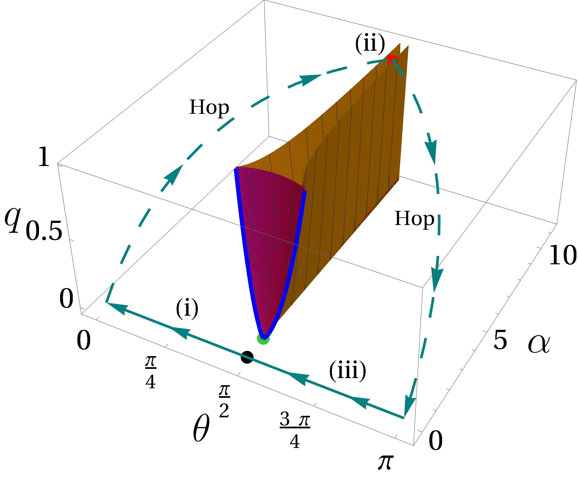
Figure 4: The hopping trajectory with $q_{0}=1$ and $\chi=+1$, cf. Eqs. (7–9), involves continuous adiabatic evolution at $q=0$ [(i), (iii)] and a relaxation-dominated evolution at $q=1$ (ii), as well as and the instantaneous hops between them. This minimizes the probability loss, while optimizing the conversion fidelity. The black dot shows the initial (and final) point of the trajectory. The entire part (ii) corresponds to the red dot ($\alpha=10,\leavevmode\nobreak\ \theta=\frac{\pi}{2},\leavevmode\nobreak\ q=1$), cf. Eq. (8).

Summary and discussion.—We have investigated the chiral state conversion under hybrid-Liouvillian dynamics. We have shown that the effect can take place in such a setting and have designed a protocol for chiral state conversion with pure target states and no probability loss.

Designing this protocol is facilitated by the fact that the EPs of a hL form a structure that continuously connects the EPs of a Lindbladian and the respective nHH. This continuity implies that the chiral state conversion effect, which is known for nHH and, separately, for Lindbladians persists even when the degree of postselection is varied during the protocol.

Our findings regarding the continuity of the EP structure are applicable to generic single-, few-, and many-body systems governed by hL. This follows from the continuous dependence of the superoperator $\mathcal{L}_{q}$ and its characteristic equation $\mathcal{C}_{q}(\lambda)$ on $q$. The EP structure continuity is a main ingredient for our near-unit-efficiency chiral state conversion protocol. Therefore, it appears likely that our protocol can be generalized to other systems as well.

With efficient many-body chiral state conversion, one might envision applying it for quantum-annealing-like computations. That is, encircling an EP structure in order to convert the system to a state that represents a solution for some problem.

The setup considered here is closely related to recent experiments investigating EPs in a superconducting qubit experiencing nHH (Naghiloo et al., 2019) and Lindbladian (Chen et al., 2021) dynamics. Continuous variation of the postselection parameter, needed for our x-adiabatic protocols, can only be done in the range $q=0.8-1$, as current efficiency of single-photon detection, which is needed for postselection, is $\lesssim 20\%$ (Minev et al., 2019). However, our hopping protocol does not suffer from this restriction and is amenable to experimental test by discontinuous switching between nHH and Lindbladian evolutions in the course of experiment.

SUPPLEMENTARY INFORMATION

I The analytical formulas for the locations of the hybrid-Liouvillian EPs

Here we present the analytical formulas for the exceptional points (EPs) of the hybrid Liouvillian $\mathcal{L}_{q}$ given in Eq. (4) of the main text.

I.1 Fourth-order degeneracies

A fourth-order degeneracy implies that the characteristic polynomial, $\mathcal{C}_{q}(\lambda)=\text{Det}(\mathcal{L}_{q}-\lambda\mathbb{\,I})$, should satisfy the following constraints: $\mathcal{C}_{q}(\lambda)=0,\,\mathcal{C}_{q}^{\prime}(\lambda)=0,\,\mathcal{C}_{q}^{\prime\prime}(\lambda)=0,\,\,\text{and}\,\,\mathcal{C}_{q}^{\prime\prime\prime}(\lambda)=0$ where ^′ denotes a derivative with respect to $\lambda$. Solving these constraints simultaneously, and denoting $\alpha=\gamma/2\omega$, we observe that there exists only one fourth-order degeneracy that is located at

$$\alpha=1,\,\theta=\frac{\pi}{2},\,q=0.$$ (10)

The Jordan decomposition of $\mathcal{L}_{q}$ at these parameters shows that this is a 3rd order EP with the fourth eigenvalue accidentally coinciding with the other three.

I.2 Third-order degeneracies

In this case, the characteristic polynomial should satisfy the following constraints: $\mathcal{C}_{q}(\lambda)=0,\,\mathcal{C}_{q}^{\prime}(\lambda)=0,\,\,\text{and}\,\,\mathcal{C}_{q}^{\prime\prime}(\lambda)=0$. Solving these three constraints simultaneously in the parameter space of $\alpha,\,\theta$ and $q$, we get two lines of third-order degeneracies, which are given by

$$\theta=\theta_{1}(\alpha),\quad q=q_{1}(\alpha),$$ (11)

and

$$\theta=\theta_{2}(\alpha)=\pi-\theta_{1}(\alpha),\quad q=q_{1}(\alpha),$$ (12)

where

$$\theta_{1}(\alpha) =\frac{1}{2}\arccos\left(\frac{\alpha^{4}-8\alpha^{2}+1}{6\alpha^{2}}\right),$$ (13)

$$q_{1}(\alpha) =-\frac{8\sqrt{6}\alpha\left(\alpha^{2}-1\right)^{3/2}}{3\left(\alpha^{4}-14\alpha^{2}+1\right)}.$$ (14)

The physical restriction on the postselection parameter, $0\leq q\leq 1$, implies that $\alpha\in[1,\sqrt{3}]$ in the above formulas. For $\alpha=1$, we have $\theta_{1}(\alpha)=\theta_{2}(\alpha)=\pi/2$ and $q_{1}(\alpha)=0$, i.e., the 3rd order degeneracy lines meet at the 4th order degeneracy, cf. Eq. (10).

Performing Jordan decomposition of $\mathcal{L}_{q}$ at the parameters corresponding to the 3rd order degeneracies, one finds that these are genuine 3rd order EPs.

I.3 Second-order degeneracies

The 2nd order degeneracies require $\mathcal{C}_{q}(\lambda)=0$ and $\mathcal{C}_{q}^{\prime}(\lambda)=0$. Solving these two constraints simultaneously in the parameter space of $\alpha,\,\theta$ and $q$, we get the surfaces parametrized as

$$q_{1}(\alpha,\theta)=\frac{\sqrt{2\eta}\left(3\left(\alpha^{2}-1\right)-\eta\right)}{3\sqrt{3}\alpha\,\sin^{2}\theta},$$ (15)

and

$$q_{2}(\alpha,\theta)=\sqrt{\frac{2}{3}}\frac{\sqrt{\left(2\left(\alpha^{2}-1\right)-\eta\right)}\left(\alpha^{2}-1+\eta\right)}{3\alpha\,\sin^{2}\theta},$$ (16)

where $\eta=\left(\alpha^{2}-1+\sqrt{\left(\alpha^{2}-1\right)^{2}-12\alpha^{2}\cos^{2}\theta}\right)$. The surface parametrized by $q_{1}(\alpha,\theta)$ is shown in purple in Fig. 1(b); the two orange surfaces in the figure are parametrized by $q_{2}(\alpha,\theta)$.

Checking the number of linearly independent eigenvectors corresponding to the degenerate eigenvalue at each of the surfaces reveals that the line $q=0$, $\theta=\pi/2$, $\alpha>1$ (i.e., $2\left(\alpha^{2}-1\right)-\eta=0$) is a trivial 2nd order degeneracy having two eigenvectors, while all the other points on the surfaces are genuine 2nd order EPs (they have only one eigenvector for the degenerate eigenvalue).