Mpemba effect in anisotropically driven inelastic Maxwell gases

Abstract

Through an exact analysis, we show the existence of Mpemba effect in an anisotropically driven inelastic Maxwell gas, a simplified model for granular gases, in two dimensions. Mpemba effect refers to the couterintuitive phenomenon of a hotter system relaxing to the steady state faster than a cooler system, when both are quenched to the same lower temperature. The Mpemba effect has been illustrated in earlier studies on isotropically driven granular gases, but its existence requires non-stationary initial states, limiting experimental realisation. In this paper, we demonstrate the existence of the Mpemba effect in anisotropically driven granular gases even when the initial states are non-equilibrium steady states. The precise conditions for the Mpemba effect, its inverse, and the stronger version, where the hotter system cools exponentially faster are derived.

1 Introduction

In recent times, there has been considerable interest in the Mpemba effect, a counterintuitive phenomenon wherein a hot system equilibrates faster than a cooler system when quenched to a low temperature. It was initially predicted for water [1, 2]. Though many reasons have been attributed to the cause of the Mpemba effect in water including convection [3], evaporation [4], dissolved gases [5], supercooling [6], hydrogen bonding [7, 8, 9] and non-equipartition of energy [10], the precise cause is still debated. One such study has even cast doubts about the existence of the Mpemba effect in water [11]. Though the Mpemba effect, as described in the case of water, involves a phase transition where the final phase is ice and the initial phase water or steam, similar Mpemba effect has been observed in other physical systems that does not involve a phase transition. The other physical systems where this effect has been demonstrated experimentally includes clathrate hydrates [12], magnetic alloys [13], polylactides [14] and more recently in colloidal systems [15, 16].

Analysis of model-based systems also shows the existence of the Mpemba effect in spin systems [17, 18, 19, 20], three state Markovian systems [21], spin glasses [22], molecular gases in contact with a thermal reservoir [23, 24, 25] and granular systems [26, 27, 28, 29, 30]. For the case of spin systems [17, 18, 19, 20] and three state Markovian systems [21], the initial probability distributions describing the hot and the cold systems correspond to their equilibrium (Boltzmann) distribution and then they are evolved to the equilibrium of the final cold temperature following the Markovian dynamics. The exact condition for the existence of the Mpemba effect is derived by analysing the distance between the probability distributions during the relaxation process. Moreover, such systems also show the existence of the inverse Mpemba effect [21] where an initially colder system can heat up faster than an initially warmer system, the strong Mpemba effect [18] where certain initial states lead to an exponentially faster cooling and also exhibit optimal heating protocols [17] in which precooling leads to faster heating. For the case of spin glasses, two systems are prepared which are in contact with different temperature thermal baths. The time evolution of their energy density (instantaneous energy per spin) is analysed to demonstrate the Mpemba effect when both the systems are quenched using a cold temperature thermal bath. For the systems of molecular gases (elastic collisions) in contact with a thermal bath [23, 24], the Mpemba effect is analysed using the mean kinetic energy of the constituent molecules. For the case of molecular gas of single species, in contact with a thermal bath [23], the Mpemba effect is due to the coupling of mean kinetic energy with the excess kurtosis of the velocity distribution function in the presence of non-linear viscous drag. On the other hand, for binary mixture of molecular gases [24, 25] in contact with a background fluid, the Mpemba effect is due to the coupling of mean kinetic energies of the individual components of the binary gas. In both cases for molecular gases, the Mpemba effect is illustrated only for non-stationary initial states.

In this paper, we focus on granular gases, a dilute composition of driven inelastic particles. Granular gases are of special interest as it is one possible area where a strong interplay between experiment and theoretical analysis for an interacting particle system is possible. At the same time, it is also an example of a system that is far from equilibrium. The Mpemba effect has been demonstrated in driven granular gases in few different contexts. To study the Mpemba effect in granular systems, two systems are prepared at two different granular temperatures (mean kinetic energy of particles). On quenching to a lower temperature (by changing the driving parameters), the Mpemba effect is said to be present if the temperatures of the two systems cross each other while relaxing to the final stationary state. For a system of smooth monodispersed particles [26], the Mpemba effect is achieved by the coupling of mean kinetic energy with the excess kurtosis of the velocity distribution function. An exact analysis was possible for the case of an inelastic Maxwell gas, wherein the rate of collision is simplified to be independent of relative velocity, and it was shown that there has to be non-trivial correlations among the initial velocities of the particles to achieve the Mpemba effect [29]. The Mpemba effect was also demonstrated for a system of rough granular gas [27], granular gas of viscoelastic particles [28] and in inertial suspensions of granular particles [31]. In all these analysis, the initial states of the systems are non-stationary for the Mpemba effect to be achieved. This is a drawback, as achieving special non-stationary states in experiments is much harder than attractive stationary states.

To achieve the Mpemba effect in a granular system with stationary initial conditions, a couple of systems have been put forward. Through an exact analysis of a driven binary granular Maxwell gases [29], it was shown that the coupling between the mean kinetic energies of the two components of the binary gas leads to the Mpemba effect, the inverse Mpemba effect and the strong Mpemba effect starting from steady state initial conditions. Here, a mechanism of driving the two types of particles differently is required, which may be difficult to achieve in practice. For a monodispersed gas in two dimensions, it was recently shown that it is possible to achieve the Mpemba effect, its inverse and the strong counterpart with initial stationary states provided the driving is anisotropic (different in the two directions) [30]. This was established based on an analysis of the Enskog-Boltzmann equation for driven granular gases with the simplifying assumption that the velocity distribution is a gaussian. By linearising the theory about the stationary states, it is shown that the Mpemba effect can be achieved by simply tuning the driving strengths, thus making it an effective system for experimental realisation of the effect. Results from event-driven simulations are consistent with the results from the linearised theory [30].

In this paper, we do an exact analysis of the system of monodispersed inelastic gas with anisotropic driving based on the inelastic Maxwell model in two dimensions. Compared to the system studied in Ref. [30] where the rate of collision is proportional to the relative velocity, in the Maxwell gas, the rate of collision is independent of the relative velocity. While this makes the Maxwell gas more unrealistic, it renders it more amenable to exact analysis, at the same time retaining the qualitative features. This advantageous feature has been exploited in obtaining more rigorous results in both freely cooling granular gas [32, 33, 34, 35] as well as in the velocity distributions of driven granular gases [36, 37, 38, 39, 40, 41, 42]. The equations for the time evolution of the relevant two point velocity correlations for the Maxwell gas form a closed set of equations [43]. We analyse these equations to determine the condition and the parameter regime for the existence of the Mpemba effect. With our exact analysis of the anisotropically driven Maxwell gas, we are able to put the results of Ref. [30], which depended on many simplifying assumptions, on a more sound footing. We show that the Mpemba and the inverse Mpemba effects exist for steady state initial conditions which can be prepared by tuning the physical parameters defining the system. In this analysis, we also demonstrate the existence of the strong Mpemba effect where for certain specific initial steady states, the equilibration rate is exponentially faster compared to any other initial steady states.

The remainder of the paper is organised as follows. Section 2 contains the definition of the model. In Sec. 3, we show that the time evolution of two point velocity-velocity correlations do not depend on higher order correlations and form a closed set of equations. This allows for an exact calculation of the steady state mean kinetic energies. In Sec. 4, we define the Mpemba effect and demonstrate its existence for an anisotropically driven granular gas. In Sec. 5, we discuss the case where driving is limited to only one direction. Section 6 contains the summary of results and discussion of their various implications.

2 The Model

Consider a monodispersed granular gas composed of $N$ identical particles. We label the particles by $i=1,\ldots,N$ and denote their two dimensional velocities by $\emph{{v}}_{\emph{{i}}}=(v_{ix},v_{iy})$. These velocities evolve in time through momentum conserving inelastic binary collisions and external driving. A pair of particles $i$ and $j$ collide at a rate $\lambda_{c}/N$. The factor $1/N$ in the collision rates ensures that the total rate of collisions between $N[N-1]/2$ pairs of particles are proportional to the system size $N$. The new velocities $\emph{{v}}^{\prime}_{\emph{{i}}}$ and $\emph{{v}}^{\prime}_{\emph{{j}}}$ are given by

$$\begin{split}\boldsymbol{v}^{\prime}_{i}=\boldsymbol{v}_{i}-\alpha[(\boldsymbol{v}_{i}-\boldsymbol{v}_{j}).\boldsymbol{\hat{e}}]\boldsymbol{\hat{e}},\\ \boldsymbol{v}^{\prime}_{j}=\boldsymbol{v}_{j}+\alpha[(\boldsymbol{v}_{i}-\boldsymbol{v}_{j}).\boldsymbol{\hat{e}}]\boldsymbol{\hat{e}},\end{split}$$ (1)

where

$$\alpha=\frac{1+r}{2},$$ (2)

$r$ being the co-efficient of restitution, and $\boldsymbol{\hat{e}}$ is the unit vector along the line joining the centres of the particles at contact. We assume that $\boldsymbol{\hat{e}}$ takes a value uniformly from $[0,2\pi)$ for each collision. In addition to collisions, the system evolves through external driving. Each particle is driven at a rate $\lambda_{d}$. During a driving event, the new velocity $\emph{{v}}^{\prime}_{\emph{{i}}}$ is given by

$$v^{\prime}_{ix}=-r_{wx}v_{ix}+\eta_{x},\quad-1<r_{wx}\leq 1,$$

$$v^{\prime}_{iy}=-r_{wy}v_{iy}+\eta_{y},\quad-1<r_{wy}\leq 1,$$ (3)

where $r_{wx}$ and $r_{wy}$ are parameters of driving and $\boldsymbol{\eta}$ is a noise taken from a fixed distribution $\Phi(\boldsymbol{\eta})$. We denote the second moment of the noise distribution by $\sigma^{2}_{x}$ and $\sigma^{2}_{y}$:

$$\sigma^{2}_{k}=\int^{\infty}_{-\infty}d\eta_{k}\eta^{2}_{k}\Phi(\boldsymbol{\eta}),\quad k=x,y.$$ (4)

Note that $\sigma^{2}_{x}\neq\sigma^{2}_{y}$ or $r_{wx}\neq r_{wy}$ corresponds to anisotropic driving and will introduce an anisotropy in the resultant velocity distribution of the particles. Such a driving scheme [Eq. (3)] leads the system to a steady state and has been used extensively in earlier studies [39, 40, 41]. The physical motivations for the form of driving may be found in Refs. [44, 43], where positive $r_{w}$’s can be identified as the coefficient of restitution of collisions between particle and a vibrating wall.

The model has two simplifying features. The spatial degrees of freedom have been neglected. This corresponds to the well-mixed limit where the spatial correlations between particles are ignored. In addition, the collision rates are independent of the relative velocity of the colliding particles. This corresponds to the so called Maxwell limit.

Let $P(\boldsymbol{v},t)$ denote the probability that a randomly chosen particle has velocity $\boldsymbol{v}$ at time $t$. Its time evolution is given by

$$\frac{d}{dt}P(\boldsymbol{v},t) =\lambda_{c}\int\int\int d\boldsymbol{\hat{e}}d\boldsymbol{v}_{1}d\boldsymbol{v}_{2}P(\boldsymbol{v}_{1},t)P(\boldsymbol{v}_{2},t)\delta(\boldsymbol{v}_{1}-\alpha[(\boldsymbol{v}_{1}-\boldsymbol{v}_{2}).\boldsymbol{\hat{e}}]\boldsymbol{\hat{e}}-\boldsymbol{v})$$

$$+\lambda_{d}\int\int d\boldsymbol{\eta}d\boldsymbol{v}_{1}\Phi(\boldsymbol{\eta})P(\boldsymbol{v}_{1},t)\delta[-r_{w}\boldsymbol{v}_{1}+\boldsymbol{\eta}-\boldsymbol{v}]-\lambda_{c}P(\boldsymbol{v},t)-\lambda_{d}P(\boldsymbol{v},t),$$ (5)

where the first and third terms on the right hand side describe the gain and loss terms due to collisions while the second and fourth terms describe the gain and loss terms due to driving.

3 Two point correlations

We are interested in the time evolution of the following two-point correlation functions:

$$E_{x}(t)=\frac{1}{N}\sum^{N}_{i=1}\langle v^{2}_{ix}(t)\rangle, C_{x}(t)=\frac{1}{N(N-1)}\sum^{N}_{i=1}\sum_{\begin{subarray}{c}j=1\\ j\neq i\end{subarray}}^{N}\langle v_{ix}(t)v_{jx}(t)\rangle,$$

$$E_{y}(t)=\frac{1}{N}\sum^{N}_{i=1}\langle v^{2}_{iy}(t)\rangle, C_{y}(t)=\frac{1}{N(N-1)}\sum^{N}_{i=1}\sum_{\begin{subarray}{c}j=1\\ j\neq i\end{subarray}}^{N}\langle v_{iy}(t)v_{jy}(t)\rangle,$$

$$E_{xy}(t)=\frac{1}{N}\sum^{N}_{i=1}\langle v_{ix}(t)v_{iy}(t)\rangle, C_{xy}(t)=\frac{1}{N(N-1)}\sum^{N}_{i=1}\sum_{\begin{subarray}{c}j=1\\ j\neq i\end{subarray}}^{N}\langle v_{ix}(t)v_{jy}(t)\rangle.$$ (6)

$E_{x}(t)$ and $E_{y}(t)$ denote the mean kinetic energies of the particles along $x$ and $y$ directions respectively. $E_{xy}(t)$ denote the correlations between $v_{x}$ and $v_{y}$ of the same particle whereas $C_{x}(t)$, $C_{y}(t)$ and $C_{xy}(t)$ denote the velocity-velocity correlations between pairs of particles. The time evolution for these correlation functions can be obtained starting from Eq. (5) [39, 40, 41, 43, 29]. These may be written compactly in a matrix form as

$$\frac{d\boldsymbol{\tilde{\Sigma}}(t)}{dt}=\boldsymbol{\tilde{R}}\boldsymbol{\tilde{\Sigma}}(t)+\boldsymbol{\tilde{D}},$$ (7)

where the column vectors $\boldsymbol{\tilde{\Sigma}}(t)$ and $\boldsymbol{\tilde{D}}$ are given by:

$$\boldsymbol{\tilde{\Sigma}}(t)=[E_{x}(t),E_{y}(t),E_{xy}(t),C_{x}(t),C_{y}(t),C_{xy}(t)]^{T},$$ (8)

$$\boldsymbol{\tilde{D}}=[\lambda_{d}\sigma^{2}_{x},\lambda_{d}\sigma^{2}_{y},0,0,0,0]^{T}.$$ (9)

While the matrix $\boldsymbol{\tilde{R}}$ can be written for any $N$, in the thermodynamic limit $N\rightarrow\infty$, it simplifies to

$$\boldsymbol{\tilde{R}}\!=\!\left[\begin{array}[]{cccccc}A_{1}+A^{xx}_{4}&A_{2}&0&-A_{1}&-A_{2}&0\\ A_{2}&A_{1}+A^{yy}_{4}&0&-A_{2}&-A_{1}&0\\ 0&0&-A_{3}+A^{xy}_{4}&0&0&A_{3}\\ 0&0&0&2A^{x}_{5}&0&0\\ 0&0&0&0&2A^{y}_{5}&0\\ 0&0&0&0&0&A^{x}_{5}+A^{y}_{5}\end{array}\right].$$ (10)

The constants $A_{1},A_{2},A_{3},A^{ij}_{4},A^{i}_{5}$ are given by:

$$\begin{split}&A_{1}=\frac{3}{4}\lambda_{c}\alpha^{4}-\lambda_{c}\alpha,\quad A_{2}=\frac{\lambda_{c}\alpha^{4}}{4},\\ &A_{3}=\lambda_{c}\alpha(1-\frac{\alpha}{2}),\quad A^{ij}_{4}=-\lambda_{d}(1-r_{wi}r_{wj}),\\ &A^{i}_{5}=-\lambda_{d}(1+r_{wi}),\quad\textnormal{where}~{}i,j\in(x,y).\end{split}$$ (11)

In the steady state, the left-hand side of Eq. (7) equals zero. After taking the thermodynamic limit ($N\rightarrow\infty$), we obtain the steady state values of the different two point correlation functions as

$$E_{x}=\frac{\lambda_{d}\big{[}\big{(}4\lambda_{d}(1-r^{2}_{wy})+\lambda_{c}\alpha(4-3\alpha)\big{)}\sigma^{2}_{x}+\alpha^{2}\lambda_{c}\sigma^{2}_{y}\big{]}}{\mathcal{F}},$$ (12)

$$E_{y}=\frac{\lambda_{d}\big{[}\big{(}4\lambda_{d}(1-r^{2}_{wx})+\lambda_{c}\alpha(4-3\alpha)\big{)}\sigma^{2}_{y}+\alpha^{2}\lambda_{c}\sigma^{2}_{x}\big{]}}{\mathcal{F}},$$ (13)

$$E_{xy}=C_{x}=C_{y}=C_{xy}=0,$$ (14)

where

$$\mathcal{F}=4\lambda_{d}^{2}(1-r^{2}_{wx})(1-r^{2}_{wy})+\alpha\lambda_{c}\lambda_{d}(4-3\alpha)(2-r^{2}_{wx}-r^{2}_{wy})+2\alpha^{2}\lambda^{2}_{c}(2-3\alpha+\alpha^{2}).$$ (15)

From the structure of $\boldsymbol{\tilde{R}}$ [see Eq. (10)], it is evident that the time evolution of velocity-velocity correlations only depend (linearly) on other velocity-velocity correlations and do not depend on the mean kinetic energies. Thus, if in the initial state, these correlations are zero, then they remain zero for all times. Since we will be considering only initial states that are stationary, the velocity-velocity correlations are initially zero [see Eq. (14)] and will continue to remain zero for all times.

We therefore set these velocity correlations to zero and write the time evolution for only the non-zero quantities, $E_{x}$ and $E_{y}$ as:

$$\frac{d\boldsymbol{\Sigma}(t)}{dt}=~{}\boldsymbol{R}\boldsymbol{\Sigma}(t)+\boldsymbol{S},$$ (16)

where

$$\boldsymbol{\Sigma}(t)=\begin{bmatrix}E_{x}(t),E_{y}(t)\end{bmatrix}^{T},$$ (17)

$$\boldsymbol{S}=\begin{bmatrix}\lambda_{d}\sigma^{2}_{x},\lambda_{d}\sigma^{2}_{y}\end{bmatrix}^{T},$$ (18)

and $\boldsymbol{R}$ is a $2\times 2$ matrix, whose entries are given by

$$\begin{split}R_{11}=&\frac{3}{4}\lambda_{c}\alpha^{2}-\lambda_{c}\alpha-\lambda_{d}(1-r^{2}_{wx}),\quad R_{12}=\frac{\lambda_{c}}{4}\alpha^{2},\\ R_{22}=&\frac{3}{4}\lambda_{c}\alpha^{2}-\lambda_{c}\alpha-\lambda_{d}(1-r^{2}_{wy}),\quad R_{21}=\frac{\lambda_{c}}{4}\alpha^{2}.\\ \end{split}$$ (19)

It is convenient to work in a different set of variables than $E_{x}(t)$ and $E_{y}(t)$. We introduce the total energy, $E_{tot}$, and the difference in energies, $E_{dif}$, as:

$$E_{tot}=E_{x}+E_{y},$$ (20)

$$E_{dif}=E_{x}-E_{y}.$$ (21)

Note that since the driving is anisotropic, $E_{dif}\neq 0$ in general.

The time evolution equations for $E_{tot}$ and $E_{dif}$ can be expressed, starting from Eq. (16), as

$$\frac{d\boldsymbol{E}(t)}{dt}=-~{}\boldsymbol{\chi}\boldsymbol{E}(t)+\boldsymbol{D},$$ (22)

where

$$\boldsymbol{E}(t)=\begin{bmatrix}E_{tot}(t),E_{dif}(t)\end{bmatrix}^{T},$$ (23)

$$\boldsymbol{D}=\begin{bmatrix}\lambda_{d}(\sigma^{2}_{x}+\sigma^{2}_{y}),\lambda_{d}(\sigma^{2}_{x}-\sigma^{2}_{y})\end{bmatrix}^{T},$$ (24)

and $\boldsymbol{\chi}$ is a $2\times 2$ matrix with the components of the matrix given by

$$\begin{split}\chi_{11}&=\frac{2\lambda_{c}\alpha(1-\alpha)+\lambda_{d}(2-r^{2}_{wx}-r^{2}_{wy})}{2},\quad\chi_{12}=\frac{\lambda_{d}(r^{2}_{wy}-r^{2}_{wx})}{2},\\ \chi_{22}&=\frac{\lambda_{c}\alpha(2-\alpha)+\lambda_{d}(2-r^{2}_{wx}-r^{2}_{wy})}{2},\quad\chi_{21}=\frac{\lambda_{d}(r^{2}_{wy}-r^{2}_{wx})}{2}.\end{split}$$ (25)

Equation (22) can be solved exactly by linear decomposition using the eigenvalues $\lambda_{\pm}$ of $\boldsymbol{\chi}$:

$$\lambda_{\pm}=\frac{1}{4}\Big{[}2\lambda_{d}(2-r^{2}_{wx}-r^{2}_{wy})+\alpha\lambda_{c}(4-3\alpha)\pm\sqrt{4\lambda^{2}_{d}(r^{2}_{wy}-r^{2}_{wx})^{2}+\alpha^{4}\lambda^{2}_{c}}\Big{]}.$$ (26)

It is straightforward to show that $\lambda_{\pm}>0$ with $\lambda_{+}>\lambda_{-}$. The solution for $E_{tot}(t)$ and $E_{dif}(t)$ is

$$\begin{split}E_{tot}(t)-\langle E_{tot}\rangle&=K_{+}e^{-\lambda_{+}t}+K_{-}e^{-\lambda_{-}t},\\ E_{dif}(t)-\langle E_{dif}\rangle&=L_{+}e^{-\lambda_{+}t}+L_{-}e^{-\lambda_{-}t},\end{split}$$ (27)

where $\langle E_{tot}\rangle$ and $\langle E_{dif}\rangle$ are steady state values of $E_{tot}(t)$ and $E_{dif}(t)$ respectively. The coefficients $K_{+},K_{-},L_{+}$ and $L_{-}$ along with $\langle E_{tot}\rangle$ and $\langle E_{dif}\rangle$ are given in Eq. (42). These coefficients depend only on the system parameters and initial conditions. Equation (27) gives the full time dependent solution for the energies, and we utilise them to demonstrate the Mpemba effect.

4 The Mpemba effect in an anisotropically driven gas

In this section, we show and determine the conditions for the existence of the Mpemba effect in the anisotropically driven monodispersed Maxwell gas based on the analysis of $E_{tot}(t)$ and $E_{dif}(t)$ [see Eq. (27)]. The Mpemba effect in granular systems has been defined as follows [26, 27, 29, 28, 30]. Consider two systems $P$ and $Q$ which have identical parameters except for the pair of driving strengths, $\sigma^{2}_{x}$ and $\sigma^{2}_{y}$. We will choose $E_{tot}$ of $P$ to be higher. Note that the systems $P$ and $Q$ are initially in steady states. We denote their steady state values for the energies by $[E^{P}_{tot}(0),E^{P}_{dif}(0)]$ and $[E^{Q}_{tot}(0),E^{Q}_{dif}(0)]$ respectively. Both the systems are then quenched to a common steady state having lower energy compared to the initial steady state energies of $P$ and $Q$. This is achieved by changing the driving strengths of $P$ and $Q$ to the common driving strengths, $\sigma^{2}_{x}$ and $\sigma^{2}_{y}$ of the final steady state, keeping all the other parameters of both the systems constant.

We say that the Mpemba effect is present if the two trajectories $E^{P}_{tot}(t)$ and $E^{Q}_{tot}(t)$ cross each other at some finite time $t=\tau$ at which

$$E^{P}_{tot}(\tau)=E^{Q}_{tot}(\tau).$$ (28)

To obtain the value of $\tau$, we equate the energies for $P$ and $Q$ from Eq. (27) to obtain

$$K^{P}_{+}e^{-\lambda_{+}\tau}+K^{P}_{-}e^{-\lambda_{-}\tau}=K^{Q}_{+}e^{-\lambda_{+}\tau}+K^{Q}_{-}e^{-\lambda_{-}\tau},$$ (29)

whose solution is

$$\tau=\frac{1}{\lambda_{+}-\lambda_{-}}\ln[\frac{K^{P}_{+}-K^{Q}_{+}}{K^{Q}_{-}-K^{P}_{-}}\Big{]}.$$ (30)

In terms of the parameters of the initial steady states, $\tau$ reduces to

$$\tau=\frac{1}{\lambda_{+}-\lambda_{-}}\ln[\frac{\chi_{12}\Delta E_{dif}-(\lambda_{-}-\chi_{11})\Delta E_{tot}}{\chi_{12}\Delta E_{dif}-(\lambda_{+}-\chi_{11})\Delta E_{tot}}\Big{]},$$ (31)

where

$$\begin{split}&\Delta E_{tot}=E^{P}_{tot}(0)-E^{Q}_{tot}(0),\\ &\Delta E_{dif}=E^{P}_{dif}(0)-E^{Q}_{dif}(0).\end{split}$$ (32)

For the Mpemba effect to be present, we require that $\tau>0$. Since $\lambda_{+}>\lambda_{-}$, the argument of logarithm in Eq. (31) should be greater than one. Simplifying, we obtain the criterion for the crossing of the two trajectories to be

$$\frac{\Delta E_{tot}}{\Delta E_{dif}}<\frac{2\lambda_{d}(r^{2}_{wy}-r^{2}_{wx})}{\lambda_{c}\alpha^{2}+\sqrt{4\lambda^{2}_{d}(r^{2}_{wy}-r^{2}_{wx})^{2}+\alpha^{4}\lambda^{2}_{c}}}.$$ (33)

The right hand side of Eq. (33) depends only on the intrinsic parameters of the system and it is always less than one (since $\alpha,\lambda_{c}>0$). On the other hand, the ratio $\Delta E_{tot}/\Delta E_{dif}$, depends on the initial steady state energies of $P$ and $Q$ [see Eq. (32)]. In the stationary state, the ratio $\Delta E_{tot}/\Delta E_{dif}$ is given by

$$\frac{\Delta E_{tot}}{\Delta E_{dif}}=\frac{\big{[}\lambda_{d}(1-r^{2}_{wy})+\alpha\lambda_{c}(2-\alpha)\big{]}\Delta\sigma^{2}_{x}+\big{[}2\lambda_{d}(1-r^{2}_{wx})+\alpha\lambda_{c}(2-\alpha)\big{]}\Delta\sigma^{2}_{y}}{2\big{[}\lambda_{d}(1-r^{2}_{wy})+\alpha\lambda_{c}(1-\alpha)\big{]}\Delta\sigma^{2}_{x}-\big{[}\lambda_{d}(1-r^{2}_{wx})+\alpha\lambda_{c}(1-\alpha)\big{]}\Delta\sigma^{2}_{y}},$$ (34)

where,

$$\Delta\sigma^{2}_{i}=(\sigma^{P}_{i})^{2}-(\sigma^{Q}_{i})^{2},\quad i\in(x,y).$$ (35)

Equation (34) shows that the ratio $\Delta E_{tot}/\Delta E_{dif}$ depends on the intrinsic parameters of the system as well as the driving strengths, $\sigma^{2}_{x}$ and $\sigma^{2}_{y}$. As a result, the driving strengths can be appropriately tuned, keeping all the other intrinsic parameters identical for both $P$ and $Q$, to prepare the initial conditions that satisfy Eq. (33). In Fig. 1(a), we consider such a situation where Eq. (33) is satisfied. Here, the systems $P$ and $Q$ have identical intrinsic parameters but the pair of driving strengths, $\sigma^{2}_{x}$ and $\sigma^{2}_{y}$, are different for the two systems. The trajectories cross at the point as predicted by Eq. (31). It is clear that though $P$ has larger initial energy than $Q$, it relaxes faster compared to the latter.

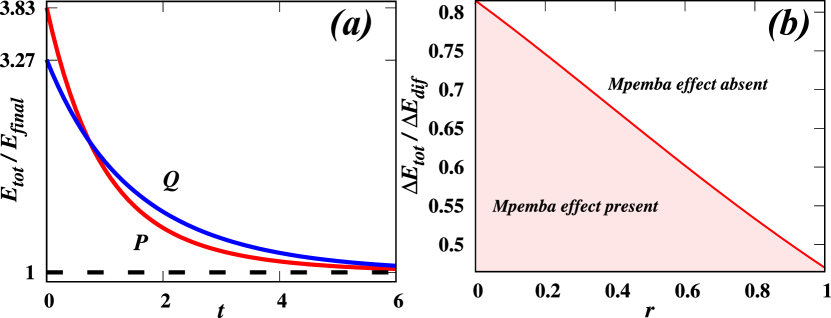
Figure 1: (a) The time evolution of the total energy, $E_{tot}(t)$ for anisotropically driven systems $P$ and $Q$ of a two dimensional inelastic Maxwell gas, driven along both the directions of the plane, with initial conditions $E^{P}_{tot}(0)$=20.27, $E^{Q}_{tot}(0)$=17.32, $E^{P}_{dif}(0)$=-7.93 and $E^{Q}_{dif}(0)$=6.26 such that $E^{P}_{tot}(0)>E^{Q}_{tot}(0)$, which satisfies the condition for the Mpemba effect as described in Eq. (33). The other parameters decribing the systems are chosen to be $r$=0.3, $r_{wx}=0.88$ and $r_{wy}=0.39$. $P$ relaxes to the steady state faster than $Q$, though its initial energy is larger. The time at which the trajectories cross each other is $\tau=0.73$ as given by Eq. (31). (b) $\Delta E_{tot}/\Delta E_{dif}$–$r$ phase diagram showing regions where the Mpemba effect is observed and $r$ is the coefficient of restitution. The line corresponds to a particular choice of the parameters $r_{wx}=0.2$, $r_{wy}=0.8$, $\lambda_{c}=1.0$ and $\lambda_{d}=1.0$. The region below the line given by Eq. (33) denotes the set of steady state initial conditions that show the Mpemba effect whereas the region on the other side of the line corresponds to initial states that do not show the Mpemba effect.

Figure 1(b) illustrates the phase space (initial conditions), based on Eq. (33), where the Mpemba effect is observable. In the figure, the line denotes the variation of right hand side of Eq. (33) with $r$, keeping all the other intrinsic parameters of the system as constant. The figure corresponds to a particular choice of the parameters $r_{wx}$, $r_{wy}$, $\lambda_{c}$ and $\lambda_{d}$. If the ratio $\Delta E_{tot}/\Delta E_{dif}$ which depends on the initial conditions of $P$ and $Q$, falls in the region below (above) the line in the phase diagram [see Fig. 1(b)], then the system exhibits (does not exhibit) the Mpemba effect.

For steady state initial conditions, the ratio $\Delta E_{tot}/\Delta E_{dif}$ is given by Eq. (34). As the ratio $\Delta E_{tot}/\Delta E_{dif}$ is a function of the driving strengths, $\sigma^{2}_{x}$ and $\sigma^{2}_{y}$ [see Eq. (34)], they can be appropriately tuned, independently for the systems $P$ and $Q$ as well as along the $x$ and $y$ directions, to access the entire region of phase space where the Mpemba effect is observable.

Note that one can introduce anisotropy in the mean kinetic energies by simply considering the case $\sigma^{2}_{x}\neq\sigma^{2}_{y}$, and keeping $r_{wx}=r_{wy}$ [see Eqs. (12) and (13)]. But in that case, the condition for the Mpemba effect reduces to $\Delta E_{tot}<0$ [see Eq. (33)] which is not possible to realise as we have assumed $\Delta E_{tot}=E^{P}_{tot}(0)-E^{Q}_{tot}(0)>0$. Therefore, to demonstrate the Mpemba effect, we restrict ourselves to the case $r_{wx}\neq r_{wy}$.

4.1 The inverse Mpemba effect

Consider now the case where a system is heated instead of being cooled unlike the direct Mpemba effect. Now if an initially colder system heats up faster than a system at an intermediate one then it is called the inverse Mpemba effect. We follow the same analysis as in the direct Mpemba effect. The condition for the inverse Mpemba effect is same as that for the direct Mpemba effect as given in Eq. (33). We prepare two systems $P$ and $Q$ such that $P$ has a higher initial total energy than $Q$ and also satisfy the condition for the inverse Mpemba effect [Eq. (33)]. We then quench both the systems to a common steady state having higher total energy compared to the initial total energies of both $P$ and $Q$. The cross-over time $\tau$ at which the trajectories $E^{P}_{tot}(t)$ and $E^{Q}_{tot}(t)$ cross is given by Eq. (31). An example is illustrated in Fig. 2.

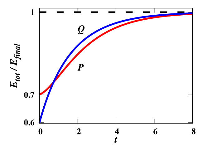
Figure 2: The time evolution of the total energy, $E_{tot}(t)$ for anisotropically driven systems $P$ and $Q$ of a two dimensional inelastic Maxwell gas, driven along both the directions of the plane, with initial conditions $E^{P}_{tot}(0)$=20.27, $E^{Q}_{tot}(0)$=17.32, $E^{P}_{dif}(0)$=-7.93 and $E^{Q}_{dif}(0)$=6.26 such that $E^{P}_{tot}(0)>E^{Q}_{tot}(0)$, which satisfies the condition for the inverse Mpemba effect as described in Eq. (33). The other parameters decribing the systems are chosen to be $r$=0.3, $r_{wx}=0.88$ and $r_{wy}=0.39$. $P$ relaxes to the steady state slower than $Q$, though its initial energy is larger. The time at which the trajectories cross each other is $\tau=0.73$ as given by Eq. (31).

The phase space of the initial steady states that satisfy the condition for the inverse Mpemba effect turns out to be the same as that for the direct Mpemba effect and is given by Eq. (34). Thus, Fig. 1(b) also illustrates the valid initial steady states given by Eq. (34) that satisfy the condition [Eq. (33)] where the inverse Mpemba effect is observable.

4.2 The strong Mpemba effect

It can be shown that there exists certain initial conditions such that the system at higher temperature relaxes to a final steady state exponentially faster compared to other initial conditions. This phenomenon is called the strong Mpemba effect. The effect may be realised when the coefficient ($K_{-}$) associated with the slower relaxation rate in the time evolution of total kinetic energy, $E_{tot}(t)$ [see Eq. (27)] vanishes.

Setting the coefficient $K_{-}$ [given by Eq. (42)] to zero, we obtain

$$E_{tot}(0)=\frac{2\lambda_{d}(r^{2}_{wy}-r^{2}_{wx})}{\lambda_{c}\alpha^{2}+\sqrt{4\lambda^{2}_{d}(r^{2}_{wy}-r^{2}_{wx})^{2}+\alpha^{4}\lambda^{2}_{c}}}E_{dif}(0)+c,$$ (36)

where

$$c=\frac{2\lambda_{d}\left[2(\sigma^{2}_{x}+\sigma^{2}_{y})+\lambda_{d}(\sigma^{2}_{x}-\sigma^{2}_{y})(r^{2}_{wx}-r^{2}_{wy})\right]}{2\lambda_{d}(2-r^{2}_{wx}-r^{2}_{wy})+\alpha\lambda_{c}(4-3\alpha)-\sqrt{4\lambda^{2}_{d}(r^{2}_{wy}-r^{2}_{wx})^{2}+\alpha^{4}\lambda^{2}_{c}}}.$$ (37)

The solution of Eq. (36) in terms of $E_{tot}(0)$ and $E_{dif}(0)$ yields the set of initial states whose relaxation is exponentially faster than the set of generic states. Among these initial states one would like to determine the ones which are steady states. The steady state ratio of $E_{tot}(0)/E_{dif}(0)$ [see Eq. (42)] for a system is given by

$$\frac{E_{tot}(0)}{E_{dif}(0)}=\frac{\begin{aligned} &\big{[}\lambda_{d}(1-r^{2}_{wy})+\alpha\lambda_{c}(2-\alpha)\big{]}\sigma^{2}_{x}+\big{[}2\lambda_{d}(1-r^{2}_{wx})+\alpha\lambda_{c}(2-\alpha)\big{]}\sigma^{2}_{y}\end{aligned}}{\begin{aligned} &2\big{[}\lambda_{d}(1-r^{2}_{wy})+\alpha\lambda_{c}(1-\alpha)\big{]}\sigma^{2}_{x}-\big{[}\lambda_{d}(1-r^{2}_{wx})+\alpha\lambda_{c}(1-\alpha)\big{]}\sigma^{2}_{y}\end{aligned}},$$ (38)

and is a function of the driving strengths, $\sigma^{2}_{x}$ and $\sigma^{2}_{y}$, as all other parameters are kept constant. One observes that the valid steady states with initial energies, $E_{tot}(0)$ and $E_{dif}(0)$ that satisfy the condition for the strong Mpemba effect [see Eq. (36)] can be obtained by appropriately tuning the driving strengths.

Thus, for a system of monodispersed Maxwell gas in two dimensions, there exists steady state initial conditions that satisfy the condition given by Eq. (36) and hence approach the final steady state exponentially faster compared to any other similar system whose initial energies lie slightly below or above the line. An example of the strong Mpemba effect is shown in Fig. 3.

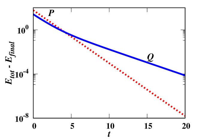
Figure 3: The time evolution of the total energy, $E_{tot}(t)$ for anisotropically driven systems $P$ and $Q$ of a two dimensional inelastic Maxwell gas, driven along both the directions of the plane, with $E^{P}_{tot}(0)=95.89$, $E^{Q}_{tot}(0)=61.57$, $E^{P}_{diff}(0)=-59.82$ and $E^{Q}_{diff}(0)=-4.26$ such that $E^{P}_{tot}(0)>E^{Q}_{tot}(0)$. These initial values satisfy both the conditions for the Mpemba effect as described in Eq. (33) as well as those for the strong Mpemba effect (for system $P$) as described in Eq. (36). The other parameters defining the system are chosen to be $r=0.2$, $r_{wx}=0.88$ and $r_{wy}=0.49$. $P$ equilibrates to the final state at an exponentially faster rate compared to $Q$ and the time at which the trajectories cross each other is $\tau=4.14$ as given by Eq. (31).

5 Special case when the driving is only in one direction

In Sec. 4, we discussed the possibility of the Mpemba effect in the case of anisotropically driven monodispersed Maxwell gas where the particles are driven along both the directions. We now consider a similar system but the driving is restricted to one direction. We follow the same analysis as in Sec. 4. Here, for the case when particles are driven only along $x$-direction (say) with driving strengths, $\sigma^{2}_{x}\neq 0$ and $\sigma^{2}_{y}=0$, the time evolution of mean kinetic energies $E_{x}$ and $E_{y}$ is

$$\begin{split}&\frac{dE_{x}(t)}{dt}=E_{x}\big{[}\lambda_{c}\alpha(\frac{3}{4}\alpha-1)-\lambda_{d}(1-r^{2}_{wx})\big{]}+E_{y}\big{[}\frac{\lambda_{c}}{4}\alpha^{2}\big{]}+\lambda_{d}\sigma^{2}_{x},\\ &\frac{dE_{y}(t)}{dt}=E_{x}\big{[}\frac{\lambda_{c}}{4}\alpha^{2}\big{]}+E_{y}\big{[}\lambda_{c}\alpha(\frac{3}{4}\alpha-1)\big{]}.\end{split}$$ (39)

The time evolution for the quantities $E_{tot}$ and $E_{dif}$ are given by Eq. (22) but now the column matrix $\boldsymbol{D}$ takes the form

$$\boldsymbol{D} =\begin{bmatrix}\lambda_{d}\sigma^{2}_{x},\lambda_{d}\sigma^{2}_{x}\end{bmatrix}^{T},$$ (40)

The solutions for $E_{tot}(t)$ and $E_{dif}(t)$ are obtained in the similar way as in Eq. (27) with the coefficients $K_{+},K_{-},L_{+}$ and $L_{-}$ along with the steady state energies $\langle E_{tot}\rangle$ and $\langle E_{dif}\rangle$ given in Eq. (43).

We now consider two systems labeled as $P$ and $Q$ with different initial conditions $[E^{P}_{tot}(0),E^{P}_{dif}(0)]$ and $[E^{Q}_{tot}(0),E^{Q}_{dif}(0)]$ where $E^{P}_{tot}(0)>E^{Q}_{tot}(0)$. Both the systems are quenched to a common steady state whose total energy is smaller than the initial total energies of $P$ and $Q$. This is achieved by changing the driving strengths of $P$ and $Q$ to the common driving strengths, $\sigma^{2}_{x}\neq 0$ and $\sigma^{2}_{y}=0$ of the final steady state, keeping all the other parameters constant for both the systems.

The condition for the Mpemba effect to be present is the same as that derived for the more general case [see Eq. (33)]. In Fig. 4(a), we consider such a situation where Eq. (33) is satisfied and hence the systems $P$ and $Q$ show the Mpemba effect. The trajectories cross at the point as predicted by Eq. (31).

In Fig. 4(b), we identify the region of phase space (initial condition) where the Mpemba effect is observable, based on Eq. (33). In the figure, the line denotes the variation of right hand side of Eq. (33) with $r$, keeping all the other intrinsic parameters of the system as constant. The figure corresponds to a particular choice of the parameters $r_{wx}$, $\lambda_{c}$ and $\lambda_{d}$. The region below the line in the phase diagram corresponds to the initial conditions $\Delta E_{tot}/\Delta E_{dif}$ [see Fig. 4(b)] that show the Mpemba effect [Eq. (33)] whereas the other region does not show the effect.

Here, we consider that the systems $P$ and $Q$ have identical intrinsic parameters once the quench is done to the common steady state. However, these intrinsic parameters that characterise the initial conditions of $P$ and $Q$ or equivalently $\Delta E_{tot}/\Delta E_{dif}$, could be different. As a result, one can tune these intrinsic parameters differently for $P$ and $Q$ to obtain initial steady states that satisfy the condition given by Eq. (33) and hence show the Mpemba effect.

However, when the intrinsic parameters other than driving strength is kept the same (both before and after the quench), the ratio $\Delta E_{tot}/\Delta E_{dif}$ for initial steady states has a simple form:

$$\frac{\Delta E_{tot}}{\Delta E_{dif}}=\frac{(2-\alpha)}{2(1-\alpha)}\geq 1.5.$$ (41)

Note that $\alpha\in[1/2,1]$ and hence the ratio in Eq. (41) is always larger than or equal to 1.5. However, we know from Eq. (33) that for the Mpemba effect to be present, $\Delta E_{tot}/\Delta E_{dif}<1$. Thus, Eq. (41) does not satisfy the required condition for the existence of the Mpemba effect. We conclude that for initial states that correspond to steady states where $P$ and $Q$ have identical intrinsic parameters except for the driving strength, the Mpemba effect is not possible when the driving is restricted to one direction.

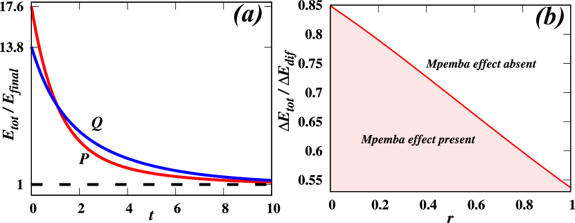
Figure 4: (a) The time evolution of the total energy, $E_{tot}(t)$ for anisotropically driven systems $P$ and $Q$ of a two dimensional inelastic Maxwell gas driven along a single direction with initial conditions $E^{P}_{tot}(0)$=28, $E^{Q}_{tot}(0)$=22, $E^{P}_{dif}(0)$=26 and $E^{Q}_{dif}(0)$=5 such that $E^{P}_{tot}(0)>E^{Q}_{tot}(0)$, which satisfies the condition for the Mpemba effect as described in Eq. (33). The other parameters decribing the systems are chosen to be $r$=0.5 and $r_{wx}=0.6$. $P$ relaxes to the steady state faster than $Q$, though its initial energy is larger. The time at which the trajectories cross each other is $\tau=1.07$ as given by Eq. (31). (b) $\Delta E_{tot}/\Delta E_{dif}$–$r$ phase diagram showing regions where the Mpemba effect is observed and $r$ is the coefficient of restitution. The line corresponds to a particular choice of the parameters $r_{wx}=0.5$, $\lambda_{c}=1.0$ and $\lambda_{d}=1.0$. The region below the line given by Eq. (33) shows the Mpemba effect whereas the region on the other side of the line does not show the Mpemba effect.

6 Summary and discussion

In this paper, we have shown an exact analysis for the existence of the Mpemba effect, the inverse Mpemba effect and the strong Mpemba effect in an anisotropically driven inelastic Maxwell gas in two dimensions. The Maxwell model for granular gases is a simplified model where the rate of collision between the granular particles is independent of their relative velocities. In addition, we assumed the well-mixed limit such that the spatial correlations were ignored. The model allows for an exact solution as the two-point velocity correlations form a coupled set of linear equations.

We show that anisotropic driving leads to the existence of the Mpemba effect starting from steady state initial conditions unlike the case of isotropic driving which required the initial conditions to be non-stationary. We considered two different cases of anisotropic driving in two dimensions: when particles are driven along one direction only and the other case where particles are driven along both the directions. In both the cases, we show that the Mpemba effect can exist for initial conditions which are valid steady states characterised by the parameters of the system. We also demonstrated the existence of the inverse Mpemba effect where a system is heated instead of being cooled. Here, an initially colder system equilibrates to a final high temperature state faster than an initially warmer system. We also derived the condition for the existence of the strong Mpemba effect where for certain initial states, a system equilibrates at an exponentially faster rate compared to any other states.

Our results place the results obtained by us in an earlier work [30] on an anisotropically driven granular gas with a more realistic velocity dependent collision rate, on a more rigorous footing. One difference between results for the two models is that in the Maxwell gas, the results depend on whether the anisotropy is applied through different driving strengths ($\sigma^{2}_{x}\neq\sigma^{2}_{y}$) or through different driving parameters ($r_{wx}\neq r_{wy}$). For the Maxwell gas, if all other parameters are kept the same, then the latter condition is necessary. This difference is due to the lack of non-linear coupling between $E_{tot}$ and $E_{dif}$ in the Maxwell model.

Appendix A Coefficients for the time evolutions of $E_{tot}$ and $E_{dif}$

In this Appendix, we solve for the time evolutions of $E_{tot}$ and $E_{dif}$ for the anisotropically driven inelastic Maxwell gas in two dimensions. We consider two cases of anisotropic driving: when the external driving is applied along both the directions with different driving strengths and another case where the driving is along one direction only as described in A.1 and A.2 respectively.

A.1 Driven along both directions of the plane

We consider an inelastic Maxwell gas in two dimensions where the particles are driven along both directions of the plane at rate $\lambda_{d}$ and with different driving strengths, $\sigma^{2}_{x}$ and $\sigma^{2}_{y}$ respectively. The time evolutions of $E_{tot}$ and $E_{dif}$ are given as in Eq. (27) where the coefficients $K_{+},K_{-},L_{+}$ and $L_{-}$ along with the steady state energies $\langle E_{tot}\rangle$ and $\langle E_{dif}\rangle$ are given by

$$K_{+} =\frac{1}{\gamma}\Big{[}-(\lambda_{-}-\chi_{11})E_{tot}(0)+\chi_{12}E_{dif}(0)-\frac{\lambda_{d}}{\lambda_{+}}\big{[}\big{(}\chi_{12}-(\lambda_{-}-\chi_{11})\big{)}\sigma^{2}_{x}-\big{(}\chi_{12}+(\lambda_{-}-\chi_{11})\big{)}\sigma^{2}_{y}\big{]}\Big{]},$$

$$K_{-} =\frac{1}{\gamma}\Big{[}(\lambda_{+}-\chi_{11})E_{tot}(0)-\chi_{12}E_{dif}(0)+\frac{\lambda_{d}}{\lambda_{-}}\big{[}\big{(}\chi_{12}-(\lambda_{+}-\chi_{11})\big{)}\sigma^{2}_{x}-\big{(}\chi_{12}+(\lambda_{+}-\chi_{11})\big{)}\sigma^{2}_{y}\big{]}\Big{]},$$

$$\langle E_{tot}\rangle =\frac{\lambda_{d}}{\gamma}\Big{[}\frac{\big{(}\chi_{12}-(\lambda_{-}-\chi_{11})\big{)}\sigma^{2}_{x}-\big{(}\chi_{12}+(\lambda_{-}-\chi_{11})\big{)}\sigma^{2}_{y}}{\lambda_{+}}-\frac{\big{(}\chi_{12}-(\lambda_{+}-\chi_{11})\big{)}\sigma^{2}_{x}-\big{(}\chi_{12}+(\lambda_{+}-\chi_{11})\big{)}\sigma^{2}_{y}}{\lambda_{-}}\Big{]},$$

$$L_{+} =\frac{1}{\gamma}\Big{[}-\frac{(\lambda_{+}-\chi_{11})(\lambda_{-}-\chi_{11})}{\chi_{12}}E_{tot}(0)+(\lambda_{+}-\chi_{11})E_{dif}(0)-\frac{\lambda_{d}}{\lambda_{+}\chi_{12}}\big{[}(\lambda_{+}-\chi_{11})(\lambda_{-}-\chi_{11})(\sigma^{2}_{x}-\sigma^{2}_{y})\big{]}\Big{]},$$

$$L_{-} =\frac{1}{\gamma}\Big{[}\frac{(\lambda_{+}-\chi_{11})(\lambda_{-}-\chi_{11})}{\chi_{12}}E_{tot}(0)-(\lambda_{+}-\chi_{11})E_{dif}(0)+\frac{\lambda_{d}}{\lambda_{-}\chi_{12}}\big{[}(\lambda_{+}-\chi_{11})(\lambda_{-}-\chi_{11})(\sigma^{2}_{x}-\sigma^{2}_{y})\big{]}\Big{]},$$

$$\langle E_{dif}\rangle =\frac{\lambda_{d}}{\chi_{12}\gamma}\Big{[}(\lambda_{+}-\chi_{11})(\lambda_{-}-\chi_{11})(\sigma^{2}_{x}-\sigma^{2}_{y})\big{(}\frac{1}{\lambda_{+}}-\frac{1}{\lambda_{-}}\big{)}\Big{]},$$

$$\gamma =\lambda_{+}-\lambda_{-}.$$ (42)

A.2 Driven along a single direction of the plane

Here, we consider an inelastic Maxwell gas in two dimensions where the particles are driven along a single direction (say along $x$ direction) at a rate $\lambda_{d}$ and with driving strengths, $\sigma^{2}_{x}\neq 0$ and $\sigma^{2}_{y}=0$. The time evolutions of $E_{tot}$ and $E_{dif}$ are given as in Eq. (27) where the coefficients $K_{+},K_{-},L_{+}$ and $L_{-}$ along with the steady state energies $\langle E_{tot}\rangle$ and $\langle E_{dif}\rangle$ are now given by

$$\begin{split}K_{+}&=\frac{1}{\gamma}\Big{[}(-\lambda_{-}+\chi_{11})E_{tot}(0)+\chi_{12}E_{dif}(0)-\frac{\chi_{12}-\lambda_{-}+\chi_{11})}{\lambda_{+}}\lambda_{d}\sigma^{2}_{x}\Big{]},\\ K_{-}&=\frac{1}{\gamma}\Big{[}(\lambda_{+}-\chi_{11})E_{tot}(0)-\chi_{12}E_{dif}(0)+\frac{\chi_{12}-\lambda_{+}+\chi_{11})}{\lambda_{-}}\lambda_{d}\sigma^{2}_{x}\Big{]},\\ \langle E_{tot}\rangle&=\frac{1}{\gamma}\Big{[}\frac{\chi_{12}-(\lambda_{-}-\chi_{11})}{\lambda_{+}}-\frac{\chi_{12}-(\lambda_{+}-\chi_{11})}{\lambda_{-}}\Big{]}\lambda_{d}\sigma^{2}_{x},\\ \langle E_{dif}\rangle&=\frac{1}{\gamma}\Big{[}\frac{(\lambda_{+}-\chi_{11})(\lambda_{-}-\chi_{11})}{\chi_{12}\lambda_{+}}-\frac{(\lambda_{+}-\chi_{11})(\lambda_{-}-\chi_{11})}{\chi_{12}\lambda_{-}}\Big{]}\lambda_{d}\sigma^{2}_{x},\\ L_{+}&=\frac{1}{\gamma}\Big{[}-\frac{(\lambda_{+}-\chi_{11})(\lambda_{-}-\chi_{11})}{\chi_{12}}E_{tot}(0)+(\lambda_{+}-\chi_{11})E_{dif}(0)-\frac{(\lambda_{+}-\chi_{11})(\lambda_{-}-\chi_{11})}{\chi_{12}\lambda_{+}}\lambda_{d}\sigma^{2}_{x}\Big{]},\\ L_{-}&=\frac{1}{\gamma}\Big{[}\frac{(\lambda_{+}-\chi_{11})(\lambda_{-}-\chi_{11})}{\chi_{12}}E_{tot}(0)-(\lambda_{-}-\chi_{11})E_{dif}(0)+\frac{(\lambda_{+}-\chi_{11})(\lambda_{-}-\chi_{11})}{\chi_{12}\lambda_{-}}\lambda_{d}\sigma^{2}_{x}\Big{]},\\ \gamma&=\lambda_{+}-\lambda_{-}.\end{split}$$ (43)

References

- [1] Lee H Meteorologica, Loeb classical library: Greek authors p.87 (Harvard University Press, Cambridge, MA, 1952)
- [2] Mpemba E B and Osborne D G 1969 Phys. Educat. 4 172–175
- [3] Vynnycky M and Kimura S 2015 Int. J. Heat Mass Transf. 80 243 – 255
- [4] Mirabedin S M and Farhadi F 2017 Int. J. Refrig. 73 219 – 225
- [5] Katz J I 2009 Am. J. Phys. 77 27–29
- [6] Auerbach D 1995 Am. J. Phys. 63 882–885
- [7] Zhang X, Huang Y, Ma Z, Zhou Y, Zhou J, Zheng W, Jiang Q and Sun C Q 2014 Phys. Chem. Chem. Phys. 16(42) 22995–23002
- [8] Tao Y, Zou W, Jia J, Li W and Cremer D 2017 J. Chem. Theory Comput. 13 55–76
- [9] Jin J and Goddard III W A 2015 J. Phys. Chem. C 119 2622–2629
- [10] Gijón A, Lasanta A and Hernández E 2019 Phys. Rev. E 100 032103
- [11] Burridge H C and Linden P F 2016 Sci. Rep. 6 37665
- [12] Ahn Y H, Kang H, Koh D Y and Lee H 2016 Korean J. Chem. Eng. 33 1903–1907
- [13] Chaddah P, Dash S, Kumar K and Banerjee A 2010 arXiv preprint arXiv:1011.3598
- [14] Hu C, Li J, Huang S, Li H, Luo C, Chen J, Jiang S and An L 2018 Cryst. Growth Des. 18 5757–5762
- [15] Kumar A and Bechhoefer J 2020 Nature 584 64–68
- [16] Kumar A, Chetrite R and Bechhoefer J 2021 arXiv preprint arXiv:2104.12899
- [17] Gal A and Raz O 2020 Phys. Rev. Lett. 124(6) 060602
- [18] Klich I, Raz O, Hirschberg O and Vucelja M 2019 Phys. Rev. X 9(2) 021060
- [19] Klich I and Vucelja M 2018 arXiv preprint arXiv:1812.11962
- [20] Das S K and Vadakkayil N 2021 Phys. Chem. Chem. Phys.
- [21] Lu Z and Raz O 2017 Proc. Natl. Acad. Sci. USA 114 5083–5088
- [22] Baity-Jesi M, Calore E, Cruz A, Fernandez L A, Gil-Narvión J M, Gordillo-Guerrero A, Iñiguez D, Lasanta A, Maiorano A, Marinari E et al. 2019 Proc. Natl. Acad. Sci. USA 116 15350–15355
- [23] Santos A and Prados A 2020 Phys. Fluids 32 072010
- [24] González R G, Khalil N and Garzó V 2020 arXiv preprint arXiv:2010.14215
- [25] González R G and Garzó V 2020 arXiv preprint arXiv:2011.13237
- [26] Lasanta A, Vega Reyes F, Prados A and Santos A 2017 Phys. Rev. Lett. 119(14) 148001
- [27] Torrente A, López-Castaño M A, Lasanta A, Reyes F V, Prados A and Santos A 2019 Phys. Rev. E 99(6) 060901
- [28] Mompó E, Castaño M, Torrente A, Reyes F V and Lasanta A 2020 arXiv preprint arXiv:2006.00241
- [29] Biswas A, Prasad V V, Raz O and Rajesh R 2020 Phys. Rev. E 102(1) 012906
- [30] Biswas A, Prasad V V and Rajesh R 2021 arXiv preprint arXiv:2104.08730
- [31] Takada S, Hayakawa H and Santos A 2021 Phys. Rev. E 103(3) 032901
- [32] Ben-Naim E and Krapivsky P L 2002 Phys. Rev. E 66(1) 011309
- [33] Baldassarri A, Marconi U M B and Puglisi A 2002 Europhys. Lett. 58 14–20
- [34] Ernst M H and Brito R 2002 Europhys. Lett. 58 182–187
- [35] Krapivsky P L and Ben-Naim E 2002 J. Phys. A 35 L147–L152
- [36] Ernst M H and Brito R 2002 Phys. Rev. E 65(4) 040301
- [37] Antal T, Droz M and Lipowski A 2002 Phys. Rev. E 66(6) 062301
- [38] Santos A and Ernst M H 2003 Phys. Rev. E 68(1) 011305
- [39] Prasad V V, Sabhapandit S and Dhar A 2014 Europhys. Lett. 104 54003
- [40] Prasad V V, Sabhapandit S and Dhar A 2014 Phys. Rev. E 90(6) 062130
- [41] Prasad V V, Das D, Sabhapandit S and Rajesh R 2017 Phys. Rev. E 95 032909
- [42] Biswas A, Prasad V V and Rajesh R 2020 J. Stat. Mech.: Theory Exp. 2020(1) 013202
- [43] Prasad V V, Das D, Sabhapandit S and Rajesh R 2019 J. Stat. Mech.: Theory Exp. 2019(6) 063201
- [44] Prasad V V and Rajesh R 2019 J. Stat. Phys. 176 1409–1433