Information theory and Electron Spin Resonance dating

Chronometric dating is becoming increasingly important in areas such as the Origin and evolution of Life on Earth and other planets, Origin and evolution of the Earth and the Solar System… Electron Spin Resonance (ESR) dating is based on exploiting effects of contamination by chemicals or ionizing radiation, on ancient matter through its absorption spectrum and lineshape. Interpreting absorption spectra as probability density functions (pdf), we use the notion of Information Theory (IT) distance allowing us to position the measured lineshape with respect to standard limiting pdf’s (Lorentzian and Gaussian). This paves the way to perform dating when several interaction patterns between unpaired spins are present in geologic, planetary, meteorite or asteroid matter namely classical-dipolar (for ancient times) and quantum-exchange-coupled (for recent times). In addition, accurate bounds to age are provided by IT from the evaluation of distances with respect to the Lorentz and Gauss distributions. Dating arbitrary periods of times  (?) and exploiting IT to introduce rigorous and accurate date values might have interesting far reaching implications not only in Geophysics, Geochronology  (?), Planetary Science but also in Mineralogy, Archaeology, Biology, Anthropology  (?), Paleoanthropology  (?, ?)…

Introduction

ESR (or EPR for Electron Paramagnetic Resonance) absorption spectroscopy is a non-interfering versatile technique that allows to explore interaction between unpaired spins and an applied magnetic field in condensed matter  (?). These unpaired spins pertain to electrons in general or electrons as well as holes in semiconducting materials. CW-ESR (Continuous wave) method measures concentrations of paramagnetic centers and free radicals by shining a sample with microwaves at a fixed frequency while simultaneously sweeping the magnetic field. Pulsed-ESR, CW-ESR successor allowed to reduce measurement time, increase sensitivity and resolution, better separate different interactions and detect different types of spin relaxation mechanisms  (?).

ESR provides precious information about local structures and dynamic processes of the paramagnetic centers within the sample under study.

Different frequencies are used such as S band (3.5 GHz), X band (9.25 GHz), K band (20 GHz), Q band (35 GHz) and W band (95 GHz). Each frequency has its own advantages and drawbacks and increasing it might increase its sensitivity. The latter is the minimal concentration of unpaired spins ESR can detect. For instance, going from the X to W band may result into a 30,000 enhancement in sensitivity. Since X band static sensitivity is around 10¹² spins/cm³ this means the detection limit is decreased to 3.33 $\times$ 10⁷ spins/cm³  (?). Other means for improving static and dynamic sensitivity (in spins/Gauss/$\sqrt{\rm Hz}$) involve reducing temperature or miniaturizing experimental parts such as the resonant cavity or even employing cQED (circuit Quantum Electrodynamics) devices such as Josephson junctions, and SQUIDS, potentially reaching single-spin sensitivity by using high quality factor superconducting micro-resonators along with Josephson Parametric Amplifiers  (?).

Importance of interest in ESR absolute dating capabilities stemmed from the fact ionizing radiation ($\alpha,\beta$ and $\gamma$) creates unpaired spins that might have extremely long lifetimes in certain materials  (?). Ionizing radiation occurs since rocks, sediments , minerals and deposits contain radioactive elements, such as potassium and isotopes produced by the ²³⁸U (Uranium), ²³⁵U (Actinium) and ²³²Th (Thorium) decay series.

Accurate dosimetry estimation is needed for radiometric dating in order to estimate how much any sample was exposed to ionizing radiation (or by extension to other processes) tying the dose absorbed by the sample to its age. More precisely, the ESR signal intensity is proportional to the paleodose $D$ (total radiation dose) given by $D=\int_{0}^{T}D_{R}(t)\,dt$ where $D_{R}(t)$ is the natural dose rate (in Grays/year) and $T$ the exposure time or estimated age  (?, ?).

Dating is important in geochronology and in Planetary Science since asteroids and meteorites contain organic materials that might provide important clues for the sources of Life on Earth  (?) and the formation of the Solar System.

It is to important to realize that ESR spectroscopy can handle radiometric dating as well as chemical dating that delivers information about various chemical processes, a mineral has been subjected to as in reference  (?).

While several other dating methodologies exist (see for instance Geyh and Schleicher  (?) or Ikeya’s book  (?)), the interest in ESR dating grew considerably after realizing its wide time range since it spans from a few thousand years to several million and even billions years which is far beyond capabilities of ¹⁴C radio-carbon dating  (?) (limited to about 50,000 years) for instance and allows to study geochronology since the formation of the Earth (about 4.5 billion years) until present time.

Historically Zeller  (?) suggested for the first time in 1968 the use of ESR for dating geological materials. In 1975 Ikeya  (?) was able to successfully date stalactite in Japanese caves with ESR and in 1978 Robins  (?) was even capable of identifying ancient heat treatment on flint artefacts with ESR.

More recently, Bourbin et al.  (?) and Gourier et al.  (?) introduced a statistical approach based on estimating an average area separating any given lineshape and the limiting Lorentz (or Breit-Wigner). This measure is a statistical correlation factor called $R_{10}$ that we show has several drawbacks and limitations. In sharp contrast, Information Theory (IT) provides distances called divergence measures that are able of tackling most of the cases a simple $R_{10}$ statistical correlation factor is unable to approach. Moreover IT provides accurate bounds to age from the evaluation of distances with respect to the limiting Lorentz and Gauss distributions.

This work is organized as follows: After describing ESR spectroscopy and spin interactions classified as dipolar or exchange, we discuss the ESR lineshapes arising in both situations then move on to the dating procedure based on the evaluation of a statistical correlation factor $R_{10}$. The latter is unable to describe several important cases (quantum exchange spin interaction or Gaussian pdf..). Thus we move on to introducing powerful IT tools based on evaluating distances (also called divergence measures or relative information entropy) between different existing pdf’s. The latter originate from the ESR lineshape by integrating it with respect to the magnetic field. Afterwards we compare these IT results to $R_{10}$ values when available. We do not address dosimetry procedures since this is beyond the goal of this work assuming that dosimetry has been tackled properly by other works.

Free Induction Decay function as a Stretched exponential

Free Induction Decay function $S(t)$ is a spin-spin correlation function yielding time-dependent interactions between magnetic moments carried by electronic spins in a material.

Since the ESR lineshape is the magnetic field derivative of $S(t)$ Fourier Transform (FT) (as explained in Supplementary Material) it is capable of of revealing these correlations.

In general, a spin system is expected to interact in two distinct ways:

1. When electrons are far apart i.e. $r\gg$ Angström (i.e. several hundred Angströms, microns and beyond) they can be considered as magnetic moments interacting in a magnetostatic fashion as $\frac{1}{r^{3}}$. This dipolar interaction  (?) is considered as classical.

2. Quantum exchange  (?) if spins are very close (typical nearest neighbor distance about a few Angströms). When electrons are close, overlap of their wavefunctions leads to short-range Slater interaction of the form $\exp(-r/r_{0})$ with $r$ the average inter-spin distance and $r_{0}$ on the order of an Angström.

Actually there is a third mixed regime called DE (Dipolar-Exchange) when inter-spin distances are intermediary between the Angström and large distances as in the classical regime. This regime  (?) which is beyond our scope is complex since it is a mixture of classical and quantum types.

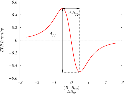
Figure 1: (Color on-line) ESR lineshape key parameters: $B_{res}$ resonance field, $A_{pp}$ peak-to-peak amplitude and corresponding linewidth $\Delta B_{pp}$.

In ESR or other resonance methods such as ferromagnetic (FMR) or nuclear magnetic resonance (NMR), there are, in general, two spin relaxation times: longitudinal $T_{1}$ (along applied external magnetic field) and transverse $T_{2}$ (perpendicular to applied external magnetic field).

In the dipolar  (?) case, Fel’dman and Lacelle  (?) have shown that spin correlation function is given by:

$$S(t)=S(0)\exp[(-t/T_{2})^{\beta(D)}]$$ (1)

with $T_{2}$ the transverse relaxation time, a measure of spin density in the sample and $\beta(D)=\frac{D}{3}$ with $D$ the dimension of geometrical spin arrangement (3 for full spatial, 2 for layers or thin films and 1 for spin chains).

In the $D=3$ dipolar case, $\beta=1$ and $S(t)=S(0)\exp[(-t/T_{2})]$ whose FT is a Lorentzian $\hat{S}(\Delta\omega)=\frac{1}{\pi}\frac{T_{2}}{[1+(\Delta\omega T_{2})^{2})]}$ where $\Delta\omega$ is frequency difference with respect to resonance frequency.

In ESR spectroscopy, the Lorentzian and the Gaussian absorption curves are considered as limiting absorption curves whose derivatives with respect to the applied field yields the ESR lineshape.

A Lorentzian appears when we have homogeneous broadening whereas a Gaussian results (in a solid) from thermal fluctuations of atomic/ionic constituents causing changes in the local magnetic field (cf Jonas review  (?)).

At lower dimensionality $D=1,2$ the rational exponent $\frac{D}{3}$ leads to a ”stretched exponential”, ”stretched Gaussian” or even ”stretched Lorentzian” (cf fig 2) dependence .

Thus ”stretched” refers to a spatial arrangement of spins in planes or layers ($D=2$) or along linear chains ($D=1$).

To summarize, $\beta=1$ yields a pure exponential with Lorentzian FT, whereas when $\beta=2$ we obtain a Gaussian with a Gaussian FT and for intermediate values $1<\beta<2$, we recover the stretched curve varieties.

Performing the FT (as detailed in Supplementary Material) using $S(t)=S(0)\exp[(-t/T_{2})^{\frac{D}{3}}]$ and $D=1,2,3,6$ to recover the stretched Lorentzian ($D=1,2$), the Lorentzian ($D=3$) and finally the Gaussian ($D=6$). In addition, one has to determine from the lineshape $A_{pp}$ and $\Delta B_{pp}$ that depend on $D,T_{2},a$ (cf. fig. 1).

ESR lineshape results displayed in fig. 2 show that we evolve from Gaussian to Lorentzian ($D=3$), to stretched Lorentzian ($D=2$) and finally stretched Lorentzian ($D=1$). Comparing to the quantum or ”spin diffusion” case (fig. 3) based on spin correlation function $S(t)=S(0)\exp[(-t/T_{2})^{\beta^{*}(D)}]$ with $\beta^{*}(D)$ function of spin arrangement dimension $D$. $\beta^{*}(1)=3/2$ in 1D (see Dietz et al.  (?)) and $\beta^{*}(2)=1$ in 2D (a simplified version of the very complex 2D case (see Richards et al.  (?)).

Classical dipolar interactions lead to spectrum broadening  (?) i.e. damping. In sharp contrast, quantum exchange among spins tends to reduce the ESR linewidth (”Exchange Narrowing” effect) and consequently, damping.

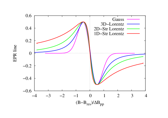
Figure 2: (Color on-line) Illustration of dipolar broadening with ESR lineshapes corresponding to spin correlation function $S(t)=S(0)\exp[(-t/T_{2})^{\frac{D}{3}}]$ for a fixed value of parameter $A_{pp}$. The Gaussian profile is the narrowest then we progress toward the broader Lorentzian ($D=3$), stretched Lorentzian ($D=2$) and finally the ($D=1$) stretched Lorentzian. Note: Str means Stretched.

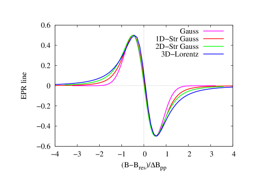
Figure 3: (Color on-line) Illustration of exchange narrowing with ESR lineshapes derived from $S(t)=S(0)\exp[(-t/T_{2})^{\beta^{*}(D)}]$ with $\beta^{*}(D)$ function of dimension $D$. Lineshapes evolve to broader (Stretched) from narrowest (Gaussian) as dimensionality increases ($D=1,2,3$) in sharp contrast with respect to the dipolar case (fig. 2). When $D=3$ the Lorentzian is recovered as in the dipolar case.

Dating with $R_{10}$ a statistical correlation measure

Characterizing the ESR lineshape around resonance, Bourbin et al.  (?) and Gourier et al.  (?) introduced a statistical method based on an average area estimation between any given lineshape and the 3D Lorentzian.

They introduced after ref.  (?, ?) functional transformations on $B$ and function $F(B)$, the derivative with respect to magnetic field of the $S(t)$) FT in order to determine age from ESR lineshape from some universal behavior.

The double scaling transformation (cf. Supplementary Material) results in a scaled magnetic field $B\rightarrow x$ and a scaled function $F(B)\rightarrow f(x)$ such that ”Lorentzian derivative” $F(B)$ corresponds to linear function $f_{L}(x)=x+3/4$ whereas ”Gaussian derivative” corresponds to $f_{G}(x)=\exp(x-1/4)$. Then a correlation factor $R_{10}$ is extracted from:

$$R_{10}=\frac{1}{10}\int_{0}^{10}[f(x)-f_{L}(x)]dx$$ (2)

meaning that the area estimation is some kind of distance measure separating the lineshape from the Lorentzian. The value 10 is the largest statistically estimated $x$ value.

When $R_{10}>0$ we have close-neighbor spins regime (quantum exchange interaction) with a mixed Gaussian-Lorentzian profile.

Finally, when $R_{10}<0$ we have distant spins (dipolar regime) in lower dimension ($D=1,2$) with a stretched Lorentzian lineshape.

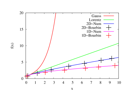
Figure 4: (Color on-line) $f(x)$ functions corresponding to the different $F(B)$. ”Lorentzian derivative” corresponds to $f_{L}(x)=x+3/4$ whereas ” Gaussian derivative” corresponds to $f_{G}(x)=\exp(x-1/4)$. Our results agree with Bourbin et al.  (?) numerical calculations.

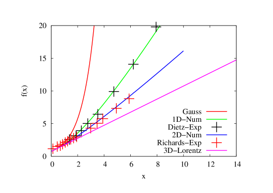
Figure 5: (Color on-line) In the quantum case $D=1,2$ curves lie between the Lorentzian and the Gaussian and our results agree with experimental data of Dietz et al.  (?) in 1D for (CH₃)₄NMnCl₃ as well as with Richards et al.  (?) in 2D for K₂MnF₄. Note: Num stands for numerical and Exp for experimental.

In the dipolar case, $x,f(x)$ diagrams (cf fig. 4) serve to identify $R_{10}>0$ region between Gaussian and Lorentzian whereas $R_{10}<0$ is below the Lorentzian.

In sharp contrast, $x,f(x)$ diagrams in the exchange case for $D=1,2$ (region $R_{10}>0$) are between the Lorentzian and the Gaussian (cf fig. 5). Thus one has to distinguish the classical dipolar from the quantum exchange case when encountering $R_{10}>0$.

Nevertheless, obtaining $R_{10}$ from ESR lineshape is interesting since it allows determination of the nature of spin interactions as quantum or classical (from $S(t)$) and their geometrical arrangement from the $D$ value as done by Bourbin et al.  (?) and Gourier et al.  (?) who considered only the classical dipolar case $D=1,2$, thus the need to examine the quantum picture (cf fig. 3).

In the intermediate dipolar case (lower dimensionality) $D=1,2$ lines are under the Lorentzian, whereas in the intermediate exchange  (?, ?) case $D=1,2$ lines are between the Gaussian and the Lorentzian.

This is important in order to obtain a reliable and precise dating assessment of rocks and sediments along the lines of Bourbin et al.  (?) and Gourier et al.  (?) who derived two different sets of age formulae from the $R_{10}$ factor.

Information theory distance measures

Introducing a measure based on Information Theory  (?) helps to discriminate between the classical and quantum pictures.

There are several divergence or distance measures between probability densities such as the Kullback-Leibler  (?, ?), squared Hellinger, $\alpha$-divergence, Jensen-Shannon, total variation  (?, ?)…(see Supplementary Material).

We choose the Cauchy-Schwarz divergence (CSD) measure  (?, ?) defined between two probability distributions $P,Q$ as:

$$D(P||Q)=-\ln\left(\int_{x\in{\mathcal{X}}}dx\;p(x)q(x)\right)+$$

$$\frac{1}{2}\ln\left(\int_{x\in{\mathcal{X}}}dx\;p^{2}(x)\right)+\frac{1}{2}\ln\left(\int_{x\in{\mathcal{X}}}dx\;q^{2}(x)\right)$$ (3)

where ${\mathcal{X}}$ is the set of values taken by continuous probability densities (pdf) $p(x),q(x),~{}x~{}\in~{}{\mathcal{X}}$.

CSD obeys several axioms of distance (see Supplementary Material) such as positivity $D(P||Q)\geq 0$, and triangle inequality: $D(P||R)\leq D(P||Q)+D(Q||R)$. It obeys also symmetry $D(P||Q)=D(Q||P)$ unlike the Kullback-Leibler (KL) measure  (?, ?) defined by:

$$D_{KL}(P||Q)=\int_{x\in{\mathcal{X}}}dx\;p(x)\ln\frac{p(x)}{q(x)}$$ (4)

Moreover CSD does not suffer from singularities whereas KL does.

The pdf are obtained from the ESR lineshape by integrating it with respect to the magnetic field (Detailed procedure is described in Supplementary Material).

In Table 1 we display CSD distances between a unit Lorentzian pdf and a set of Dipolar and Exchange pdf along with the $R_{10}$ factor and corresponding ages.

In Table 2 we display CSD distances between a unit Gaussian and a set of Dipolar and Exchange pdf along with the $R^{*}_{10}$ factor and corresponding ages that would correspond to formula:

$$R^{*}_{10}=\frac{1}{10}\int_{0}^{10}[f(x)-f_{G}(x)]dx,\,f_{G}(x)=\exp(x-1/4)$$ (5)

Actually, we did not use the above formula and rather extrapolated the Lorentzian $R_{10}$ values to estimate the age by modifying Bourbin  et al. coefficient $\alpha_{B}$. In addition we provide an experimental method (in Supplementary Material) to determine age and evaluate its bounds based on (CSD) distances $d_{L}$ and $d_{G}$ with respect to unit Lorentzian and Gaussian distributions labeled as $p(x)$ as well as from $\sigma_{q}$ the standard deviation of $q(x)$ corresponding to the measured ESR spectrum. Finally, age is expressed with the formula $10^{A_{L,G}}$ where $A_{L,G}=d_{L,G}^{\xi}\sigma_{q}^{\eta}$ with exponents $(\xi,\eta)$ determined by optimization (procedure detailed in Supplementary Material).

Lorentzian $P$	$D(P||Q)$	$R_{10}$	Age (Gyr)
Dipolar pdf $Q$
$D=1$ Str Lorentz	0.21	-2.94	3.54
$D=2$ Str Lorentz	2.50 $\times 10^{-2}$	-1.94	2.74
$D=3$ Lorentz	1.19 $\times 10^{-6}$	0.0	1.67
Gauss	2.55 $\times 10^{-2}$	1.71 $\times 10^{3}$	Undefined
Exchange pdf $Q$
$D=1$ Str Gauss	1.14 $\times 10^{-2}$	6.78	0.29
$D=2$ Str Gauss	4.12 $\times 10^{-3}$	2.30	0.93
$D=3$ Lorentz	1.19 $\times 10^{-6}$	0.0	1.67
Gauss	2.55 $\times 10^{-2}$	1.71 $\times 10^{3}$	Undefined

Table 1: Cauchy-Schwarz distances separating a unit width $P$ Lorentzian and $Q$ distributions (Dipolar and Exchange) with corresponding $R_{10}$ factor yielding age in Gyr (Giga or billion years). Age in years is deduced from Bourbin  et al.  (?) formula $10^{\left(\frac{R_{10}-\beta_{B}}{\alpha_{B}}\right)}$ with $\alpha_{B}=-9.$ and $\beta_{B}=83.$. Note that Skrzypczak  et al.  (?) define another set of coefficients: $\alpha_{S}=-5.3$ and $\beta_{S}=48.9$ (Other examples are detailed in Supplementary Material).

Gaussian $P$	$D(P||Q)$	$R^{*}_{10}$	Age (Myr)
Dipolar pdf $Q$
$D=1$ Str Lorentz	0.25	-2.94	90.59
$D=2$ Str Lorentz	5.11 $\times 10^{-2}$	-2.89	89.61
$D=3$ Lorentz	1.51 $\times 10^{-2}$	2.73	27.09
Gauss	0.0	0.0	48.44
Exchange pdf $Q$
$D=1$ Str Gauss	1.86 $\times 10^{-2}$	-5.02 $\times 10^{-2}$	48.96
$D=2$ Str Gauss	1.44 $\times 10^{-2}$	3.51	22.91
$D=3$ Lorentz	1.51 $\times 10^{-2}$	2.73	27.09
Gauss	0.0	0.0	48.44

Table 2: Cauchy-Schwarz distances separating a unit standard deviation $P$ Gaussian and $Q$ distributions (Dipolar and Exchange). The corresponding $R^{*}_{10}$ factor is obtained from extrapolating the above Lorentzian $R_{10}$ value and the age obtained in Myr (Mega or million years) is deduced from altering the Bourbin  et al. coefficient $\alpha_{B}$ (Other examples are detailed in Supplementary Material).

In this work we developed an ESR lineshape based chronometric dating methodology handling both Dipolar (classical) and Exchange (quantum) interactions between unpaired spins.

It is based on evaluating IT distances (divergence measures) between a Lorentzian or a Gaussian (analytical) pdf’s and an experimental pdf obtained from the measured ESR lineshape integrated over the applied magnetic field.

From the ESR detection point of view, ancient material age is extracted with FT of a spin-correlation function $S(t)$ pertaining to unpaired interacting spins that might have extremely long lifetimes and originate from ($\alpha,\beta$ and $\gamma$) ionizing radiation.

$S(t)$ is of a stretched exponential form with a characteristic exponent $\beta(D)$ that depends on unpaired spin arrangement dimension $D$.

In the dipolar interaction case, $\beta(D)=\frac{D}{3}$ according to Fel’dman  et al.  (?) whereas in the exchange interaction case, Dietz  et al.  (?) and Richards  et al.  (?) found $\beta^{*}(D=1)=3/2$ and $\beta^{*}(D=2)=1$ respectively (in the ”spin diffusion” case).

Considering aging as an evolutionary IT distance (or relative information entropy) between pdf’s stemming from ESR lineshapes integrated with respect to the applied magnetic field brings a major paradigm shift to chronometric dating.

IT provides an alternate look at dating based on using distances (with respect to Gaussian, Lorentzian…) as well as arbitrary coupling between spins (dipolar, exchange…) paving the way to cover any period of time with the proviso of having performed previously an appropriate dosimetry analysis. IT approach might be further extended to the intermediary Dipolar-Exchange regime where classical and quantum interactions are intertwined.

Supplementary Materials

Materials and Methods

ESR absorption spectroscopy reveals time-dependent interactions between electronic spins carrying magnetic moments in a material as reflected in the correlation function $S(t)$ also called Free Induction Decay function.

The ESR lineshape is the field derivative of $S(t)$ Fourier Transform (FT). An example is shown in the case of the Lorentzian in fig. S1.

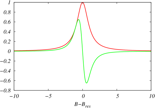
Figure S1: (Color on-line) absorption line (in red) and its field derivative the ESR lineshape (in green) in the Lorentzian case.

Magnetic resonance at a field $B_{res}$ is such that frequency $\omega=\gamma B$ where $\gamma$ is gyromagnetic ratio given by $\gamma=\mu_{0}g_{L}e\hbar/2m_{e}$ ($\mu_{0}$= vacuum permeability, $g_{L}=$ Landé factor, $e,m_{e}=$ charge and electron mass). This implies $\Delta\omega\propto B-B_{res}$ with $B$ (applied field) and resonance field $B_{res}$.

When $S(t)=S(0)\exp[(-t/T_{2})]$ its FT is a Lorentzian in $B$ such that: $\hat{S}(B)=\frac{1}{\pi}\frac{1}{\left[1+\left(\frac{B-B_{res}}{\Delta B_{pp}}\right)^{2}\right]}$.

In the general case, ESR lineshape is obtained by taking the derivative with respect to applied field $B$) of $\hat{S}(B)$ such that $F(B)=\frac{d\hat{S}(B)}{dB}$. Note that $\hat{S}(B)$ is often denoted as the ESR power absorption, the imaginary part of the generalized susceptibility $\chi"(B)$.

$S(t)$ FT is written as $\hat{S}(\omega)=\int_{0}^{+\infty}e^{-i\omega t}S(t)dt$.

In ESR, $\omega$ is proportional to the applied magnetic field allowing us to replace $\omega$ by $B-B_{res}$ resulting in $\hat{S}(B-B_{res})=\int_{0}^{+\infty}e^{-ia(B-B_{res})t}S(t)dt$ with $a=g_{L}\mu_{B}/\hbar$, $g_{L}$ the Landé factor, $\mu_{B}$ Bohr magneton and $\hbar$ Planck constant.

ESR lineshape $F(B)$ is obtained from the derivative with respect to $B$ of $\hat{S}(B-B_{res})$ yielding:

$$F(B) = Re\left[\int_{0}^{+\infty}\frac{d}{dB}e^{-ia(B-B_{res})t}S(t)dt\right]$$ (S1)

$$= -a\int_{0}^{+\infty}t\sin[a(B-B_{res})t]S(t)dt$$

Hence it suffices to evaluate the above integral using $S(t)=S(0)\exp[(-t/T_{2})^{\frac{D}{3}}]$ and $D=1,2,3,6$ to recover the stretched Lorentzian ($D=1,2$), the Lorentzian ($D=3$) and finally the Gaussian ($D=6$).

Integrating requires special methods to reduce errors resulting from large number of oscillations emanating from the term $\sin[a(B-B_{res})t]$. We have used a number of numerical algorithms  (?) in order to obtain accurate and reliable results  (?, ?, ?).

In order to characterize the ESR lineshape around resonance, Bourbin et al.  (?) and Gourier et al.  (?) introduced a statistical method based on an average area estimation between any given lineshape and the 3D Lorentzian.

They introduced after ref.  (?, ?) a double scaling transformation acting on the magnetic field $B$ and the ESR lineshape $F(B)$ such that:

$$x = \left(\frac{B-B_{res}}{\Delta B_{pp}}\right)^{2},$$

$$y = f(x)=\sqrt{\frac{A_{pp}}{|F(B-B_{res})|}\frac{|B-B_{res}|}{\Delta B_{pp}}}$$ (S2)

For example, ”Lorentzian derivative” $F(B)$ corresponds to linear function $f_{L}(x)=x+3/4$ whereas ”Gaussian derivative” corresponds to $f_{G}(x)=\exp(x-1/4)$.

Dating is based on a statistical correlation factor $R_{x_{m}}$ extracted from the integral:

$$R_{x_{m}}=\frac{1}{x_{m}}\int_{0}^{x_{m}}[f(x)-f_{L}(x)]dx$$ (S3)

where $x_{m}$ is some assumed large $x$ value such that the area estimated lying between $f(x)$ and $f_{L}(x)]$ is a distance measure separating the ESR lineshape from the Lorentzian.

Note that it is possible to determine another statistical correlation factor $R^{*}_{x_{m}}$ extracted from the integral:

$$R^{*}_{x_{m}}=\frac{1}{x_{m}}\int_{0}^{x_{m}}[f(x)-f_{G}(x)]dx$$ (S4)

where the area value indicates how much the ESR lineshape differs from the Gaussian.

Information theory effective distance measure

Information Theory (IT) provides an effective distance  (?) or a divergence measure separating two functions (in this case probability density functions or pdf) to enable their comparison not only from the geometrical shape point of view but also from the information content as well.

Going from a distance connecting two points to one linking two functions helps determine how much the functions are dissimilar in several ways (analytical, geometrical and informational). That is why $D(P||Q)$ is also called relative information entropy that does not behave as a metric but rather as the square of the Euclidian one  (?).

Several examples of $D(P||Q)$ are displayed in Table S1.

Distance $D(P||Q)$	Definition
Squared Hellinger	$\int_{x\in{\mathcal{X}}}dx\;(\sqrt{p(x)}-\sqrt{q(x)})^{2}$
Squared triangular	$\int_{x\in{\mathcal{X}}}dx\;\frac{(q(x)-p(x))^{2}}{p(x)+q(x)}$
Squared perimeter	$\int_{x\in{\mathcal{X}}}dx\;\sqrt{p^{2}(x)+q^{2}(x)}-\sqrt{2}$
$\alpha$-divergence	$\frac{4}{1-\alpha^{2}}\left(1-\int_{x\in{\mathcal{X}}}dx\;p^{\frac{1-\alpha}{2}}(x)q^{1+\alpha}(x)\right)$
Jensen-Shannon	$\frac{1}{2}\int_{x\in{\mathcal{X}}}dx\;\left(p(x)\ln\frac{2p(x)}{p(x)+q(x)}+q(x)\ln\frac{2q(x)}{p(x)+q(x)}\right)$
Pearson $\chi^{2}_{P}$	$\int_{x\in{\mathcal{X}}}dx\;\frac{(q(x)-p(x))^{2}}{p(x)}$
Neyman $\chi^{2}_{N}$	$\int_{x\in{\mathcal{X}}}dx\;\frac{(q(x)-p(x))^{2}}{q(x)}$
Total variation (metric)	$\frac{1}{2}\int_{x\in{\mathcal{X}}}dx\;|p(x)-q(x)|$

Table S1: Examples of Information Theory distances between two pdf $p(x),q(x)$. Note that $\alpha$-divergence, Pearson $\chi^{2}_{P}$ and Neyman $\chi^{2}_{N}$ do not satisfy the axiomatic symmetry requirement of a distance $D(P||Q)=D(Q||P)$.

The Cauchy-Schwarz distance (CSD) measure  (?, ?) is convenient since it obeys the axioms of distance and is free of singularities (see main article).

ESR absorption spectra when interpreted as a pdf (see fig. S1 for the Lorentzian case), is considered as modified by aging due to time-dependent interactions between electronic spins in an archaeological material.

The time correlation function $S(t)$ (Free Induction Decay function) yields the ESR lineshape $F(B)$ since it is the field derivative of its Fourier Transform (FT).

Thus an IT distance could be used as a measure of aging induced by ionizing radiation and this supplement details and illustrates the procedure for carrying the dating method.

Experimental protocols for dating with IT distance

Experimentally, two procedures are possible:

1. Direct treatment of the absorption spectra considered as a pdf and evaluating the IT distance with respect to a given reference (Lorentzian, Gaussian…).

2. Extraction of the absorption spectra from the measured ESR lineshape $F(B)$ by integrating it with respect to the applied field $B$ and afterwards evaluating the IT distance.

The extraction of the absorption spectrum from ESR lineshape $F(B)$ entails several steps:

1. Spline interpolation of the ESR lineshape $F(B)$.

2. Symmetrization of the ESR lineshape using shifting by $\delta$ such that $\int F(B)dB=\delta\int dB$.

3. Field integration of the symmetrized ESR lineshape to get the absorption spectrum.

4. Filtering (smoothing) of the absorption spectrum.

5. Normalization of the absorption spectrum and transformation into a pdf $p(x)$ with $x=\left(\frac{B-B_{res}}{\Delta B_{pp}}\right)$.

After transformation of the ESR lineshape into a pdf, the evaluation of the CSD measure  (?, ?) can be undertaken to determine the age from the evaluation of the CSD measure taken between the different probability distributions  (?, ?, ?) corresponding to the ESR spectrum and the Lorentzian or Gaussian considered as limiting distributions.

Age is determined from (CSD) distances $d_{L}$ and $d_{G}$ with respect to unit Lorentzian and Gaussian distributions labeled as $p(x)$ as well as from $\sigma_{q}$ the standard deviation of $q(x)$ corresponding to the measured ESR spectrum. Age is evaluated with the formula $10^{A_{L,G}}$ where $A_{L,G}=d_{L,G}^{\xi}\sigma_{q}^{\eta}$ for the Gyr (Giga or billion year), Myr (Mega or million year) cases whereas it is given by $A_{L,G}=d_{L,G}^{\zeta}\sigma_{q}^{\eta}$ for the Kyr (thousand year) cases with $d=d_{L}$ in the Lorentz or $d=d_{G}$ in the Gaussian case. Exponents $\xi$=-1.28, $\eta=2.74\times 10^{-2}$, $\zeta=$-0.32 are determined by optimization (see Table S2).

Sample	$d_{L}$	$d_{G}$	$\sigma_{q}$	Lorentz Age	Gauss Age
Gunflint  (?)	0.18	0.23	8.17	2.34 Gyr	8.91 $\times 10^{-3}$ Gyr
B4  (?)	0.21	0.21	0.77	8.51 Myr	11.78 Myr
Enamel  (?)	1.49 $\times 10^{-2}$	1.17 $\times 10^{-2}$	1.60	7.29 Kyr	14.47 Kyr

Table S2: Age is evaluated with the formula $10^{A_{L,G}}$ where $A_{L,G}=d_{L,G}^{\xi}\sigma_{q}^{\eta}$ for the Gyr, Myr cases whereas it is given by $A_{L,G}=d_{L,G}^{\zeta}\sigma_{q}^{\eta}$ for the Kyr cases with $d=d_{L}$ for the Lorentz case or $d=d_{G}$ for the Gaussian case.

We illustrate the Information Theory dating procedure with a first example pertaining to Gunflint from Schreiber beach locality (Port Arthur Homocline) in Ontario Canada.

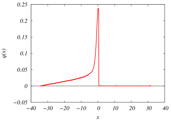
Figure S2: (Color on-line) Absorption line obtained from the ESR lineshape Gunflint sample taken from Skrzypczak PhD thesis  (?) fig.II.25

After extracting the absorption spectrum from the ESR lineshape, we find the CSD between Skrzypczak Gunflint  (?) $q(x)$ and a unit Lorentzian $p(x)$ as 0.18 whereas it is 0.23 between $q(x)$ and a unit Gaussian $p(x)$.

In order to extract the age based on the $R_{10}$ evaluation as explained in the main work, we find: $R_{10}$= -1.765 with age=2.62 Gyr. Lorentz and Gauss CSD ages are 2.34 Gyr and 8.91 $\times 10^{-3}$ Gyr respectively (cf. Table S2) whereas Skrzypczak-Bonduelle estimated it to be about 1.88 Gyr (Gyr) in her PhD thesis  (?).

Another example is a latosol sediment called B4 drawn from Balan et al.  (?) fig.2 and extracted from 100 cm depth at a site 60 km North of the city of Manaus capital of Amazonas state in North-Western Brazil.

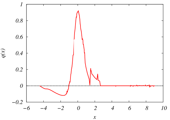
Figure S3: (Color on-line) Absorption line obtained from the ESR lineshape B4 latosol sediment of Balan et al.  (?) fig.2. The negative wing of the pdf is taken care of by upward shifting of the curve.

The age is determined from the $R_{10}$ evaluation obtained as $R_{10}$= -0.575 with age=1.932 Gyr Using the extrapolated procedure outlined in the main text, we get an age= 54.75 Mega-years (Myr). Lorentz and Gauss CSD ages are 8.51 Myr and 11.78 Myr respectively (cf. Table S2) whereas Balan et al.  (?) estimated it around 23.9 Myr.

The third example is drawn from Jonas  (?) who worked extensively on fossil tooth enamel dating (spanning several hundred thousand years up to 2 Myr).

From the ESR lineshape (calibrated spectrum of fig.7), we extract the absorption line according to the above protocol with the result displayed in fig. S4.

Figure S4: (Color on-line) absorption line obtained from the fossil tooth enamel ESR lineshape of Jonas  (?) fig.7. The negative part of the pdf is treated as in the B4 sediment case.

We find the CSD between a Lorentzian (resp. Gaussian) $p(x)$ and Jonas  (?) based $q(x)$ as 1.49 $\times 10^{-2}$ and 1.17 $\times 10^{-2}$ yielding respective ages 7.29 Kyr and 14.47 Kyr.

For the sake of comparison, if we use the $R_{10}$= -3.26 value (not to be used for the tooth enamel era but for ancient carbonaceous matter as in Bourbin  et al.  (?)), we get an age of 3.84 Gyr, a value larger than 3.5 Gyr the maximum accepted age of organic matter. On the other hand, if we use the interpolation method we get 97.08 Myr which is beyond the 2 Myr limiting age of fossil tooth enamel.

References

- 1. R. S. Anderson, S. P. Anderson, Dating methods, and establishing timing in the landscape (Cambridge University Press, 2010).
- 2. J.-J. Bahain, et al., Quaternaire 18, 175 (2007).
- 3. M. J. Aitken, C. B. Stringer, P. A. M. (ed), The Origin of Modern Humans and the Impact of Chronometric Dating (Princeton University Press, (Princeton, NJ), 1993).
- 4. R. A. Taylor, Analytical Chemistry 59, 317A (1987).
- 5. D. Richter, G. A. Wagner, Chronometric Methods in Palaeoanthropology (Springer-Verlag, Berlin, 2014).
- 6. M. J. Aitken, Reports on Progress in Physics 62, 1333 (1999).
- 7. A. Schweiger, Angewandte Chemie International Edition in English 30, 265 (1991).
- 8. N. Chen, Y. Pan, J. A. Weil, M. J. Nilges, American Mineralogist 87, 47 (2002).
- 9. S. Probst, et al., Applied Physics Letters 111, 202604 (2017).
- 10. A. R. Skinner, Applied Radiation and Isotopes 52, 1311 (2000).
- 11. E. J. Rhodes, Annual Review of Earth and Planetary Sciences 39, 461 (2011).
- 12. M. Ikeya, New Applications of Electron Spin Resonance-Dating, Dosimetry and Microscopy (World Scientific, 1993).
- 13. M. Jonas, Radiation Measurements 27, 943 (1997).
- 14. G. A. Wagner, et al., PNAS 107, 19726 (2010).
- 15. M. A. Geyh, H. Schleicher, Absolute Age Determination Physical and Chemical Dating Methods and Their Application (Springer-Verlag, Berlin, 1990).
- 16. I. Galli, et al., Physical Review Letters 107 (2011).
- 17. E. Zeller, Thermoluminescence of Geological Materials (Academic, London, 1968).
- 18. G. V. Robins, N. J. Seely, D. A. C. McNeil, M. R. C. Symons, Nature 276, 703 (1978).
- 19. M. Bourbin, et al., Astrobiology 13, 151 (2013).
- 20. A. Skrzypczak-Bonduelle, et al., Applied Magnetic Resonance 33, 371 (2008).
- 21. J. V. Vleck, Physical Review 74, 1168 (1948).
- 22. A. Bencini, D. Gatteschi, Exchange narrowing in lower dimensional systems (Springer-Verlag, Berlin, 1990).
- 23. B. A. Kalinikos, A. N. Slavin, Journal of Physics C: Solid State Physics 19, 7013 (1986).
- 24. E. B. Fel’dman, S. Lacelle, The Journal of Chemical Physics 104, 2000 (1996).
- 25. R. E. Dietz, et al., Physical Review Letters 26, 1186 (1971).
- 26. P. M. Richards, M. B. Salamon, Physical Review B 9, 32 (1974).
- 27. C. Kittel, E. Abrahams, Physical Review 90, 238 (1953).
- 28. T. M. Cover, J. A. Thomas, Elements of Information Theory (John Wiley and Sons, 1991).
- 29. W. H. Press, S. A. Teukolsky, W. T. Vetterling, B. P. Flannery, Numerical Recipes: The Art of Scientific Computing (Cambridge University Press, USA, 2007), third edn.
- 30. D. Morales, E. L. Pardo, M. Salicrù, M. L. Menéndez, J. Stat. Plann. Inference 38, 201 (1994).
- 31. A. Skrzypczak-Bonduelle, Les premières traces de vie sur terre : une approche spectroscopique et mimétique du problème, Ph.D. thesis, Université Paris VI (2005).
- 32. E. Balan, et al., Geochimica et Cosmochimica Acta 69, 2193 (2005).
- 33. E. Helfand, Journal of Chemical Physics 78, 1931 (1983).
- 34. E. W. Montroll, J. T. Bendler, Journal of Statistical Physics 34, 129 (1984).
- 35. J. Wuttke, arXiv.org pp. 1–11 (2009).