TOI-220 $b$: a warm sub-Neptune discovered by TESS

Abstract

In this paper we report the discovery of TOI-220 $b$, a new sub-Neptune detected by the Transiting Exoplanet Survey Satellite (TESS) and confirmed by radial velocity follow-up observations with the HARPS spectrograph. Based on the combined analysis of TESS transit photometry and high precision radial velocity measurements we estimate a planetary mass of 13.8 $\pm$ 1.0 M_⊕ and radius of 3.03 $\pm$ 0.15 R_⊕, implying a bulk density of 2.73 $\pm$ 0.47 $\textrm{g\,cm}^{-3}$. TOI-220 $b$ orbits a relative bright (V=10.4) and old (10.1$\pm$1.4 Gyr) K dwarf star with a period of $\sim$10.69 d. Thus, TOI-220 $b$ is a new warm sub-Neptunes with very precise mass and radius determinations. A Bayesian analysis of the TOI-220 $b$ internal structure indicates that due to the strong irradiation it receives, the low density of this planet could be explained with a steam atmosphere in radiative-convective equilibrium and a supercritical water layer on top of a differentiated interior made of a silicate mantle and a small iron core.

1 Introduction

Launched in April 2018, the Transiting Exoplanet Survey Satellite (TESS) space mission (Ricker et al., 2015) has discovered about 98 confirmed new exoplanets and more than 2450 candidates. Among all the confirmed exoplanets, one class of particular interest are the small-sized planets (R $<$ 5 R_⊕) orbiting bright stars (V $<$ 11 mag) with periods shorter than 10 days. Within this parameter space there is the so-called Neptunian desert (Szabó & Kiss, 2011; Mazeh et al., 2016), which is a region that presents a significant paucity of hot/highly irradiated planets with respect to the overall planet population. This deficit could be seen as evidence of photoevaporation and/or tidal disruptions (Owen & Lai, 2018) or of core-powered atmospheric mass loss mechanism (Ginzburg et al., 2018; Gupta & Schlichting, 2019). Currently, of all the known planets in the Neptunian desert only a very small number have precisely measured masses (e.g. West et al., 2019; Armstrong et al., 2020; Jenkins et al., 2020), preventing a comprehensive understanding of the formation history of these objects. On the other side, there is a population of sub-Neptune size planets exposed to a milder stellar irradiation that usually present a gas-rich envelope with equilibrium temperatures below 1000 K (e.g. Morley et al., 2015; Crossfield & Kreidberg, 2017; Gao et al., 2020). In this paper we present the discovery and confirmation of TOI-220 $b$, a sub-Neptune orbiting TYC 8897-01263-1, an old (10.1 Gyr) K0 V high proper motion southern star with a magnitude of 9.69 in the TESS bandpass (V=10.47). The brightness of the star, therefore, enabled a precise high SNR radial velocity (RV) follow-up campaign with the High Accuracy Radial velocity Planet Searcher (HARPS, Pepe et al., 2002) spectrograph mounted at the ESO La Silla 3.6 m telescope, in the framework of the NCORES (e.g., Nielsen et al., 2020; Armstrong et al., 2020) and KESPRINT (e.g., Gandolfi et al., 2018; Carleo et al., 2020) collaborations. The confirmation of the planetary nature of TOI-220 $b$ is based on the simultaneous analysis of the TESS photometry and HARPS RV measurements.

The rest of the paper is organized as follows. The gathered observations of the TOI-220 system are described in Sect. 2. The stellar analysis, the combined modelling and the timing analysis of the transits are presented in Sect. 3. In Sect. 4 we describe the Bayesian analysis of the internal structure of TOI-220 $b$ and the final discussion is presented in Sect. 5.

2 Observations

2.1 TESS observations

During TESS Southern ecliptic hemisphere observations, TOI-220 was observed through sectors 1–12 with the exception of sector 3. By the end of the writing of this work, the sectors 27 and 28 light curves were released, as part of the TESS extended survey in the Southern hemisphere. These data were included in the timing analysis (Sect. 3.4) and in the search for transits of the hypothetical planet $c$ (Appendix C). The transit signals of TOI-220.01 (aka TOI-220 $b$) were detected by the TESS Science Processing Operations Center (SPOC, Jenkins et al., 2016) transit search pipeline (Jenkins, 2002; Jenkins et al., 2010; Li et al., 2019). The transit detection threshold crossing event, with a periodicity of 10.695 d, a depth of $\sim$900 ppm, and a SNR$\sim$28, subsequently passed all SPOC data validation diagnostic tests (Twicken et al., 2018) and was promoted to TESS Object of Interest (TOI) status as a planet candidate (Guerrero et al., submitted). For each TESS sector, the light curve of the target was retrieved from the Mikulski Archive for Space Telescopes (MAST) archive. In this work, the two-minute cadence Presearch Data Conditioning Simple Aperture Photometry (PDCSAP) light curves (Stumpe et al., 2012; Stumpe et al., 2014; Smith et al., 2012) detrended with the SPOC algorithms were used. Two or three transits of TOI-220 $b$ were identified using a simple Box Least Squares (BLS) analysis on per-Sector light curves. After a first inspection of the flux time series of each sector some transits of TOI-220 $b$ were discarded due to SNR considerations and/or due to large systematics in the flux time series. This was the case for the full light curve of Sector 11. A few transits with poor coverage (incomplete transits) were also discarded. Therefore, only one or two transits per TESS Sector were finally extracted. A total of 17 out of the 24 transits of TOI-220 $b$ observed by TESS were considered for further analysis. After a first estimation of the individual time of transits using the period obtained from the BLS analysis, we extracted the photometric light curves around 0.4 days before/after the transit central time, when possible. The TESS sector, central time, and the 2 min RMS of each transit used in this work are reported in Table 1 and the light curves are shown in Fig. 1.

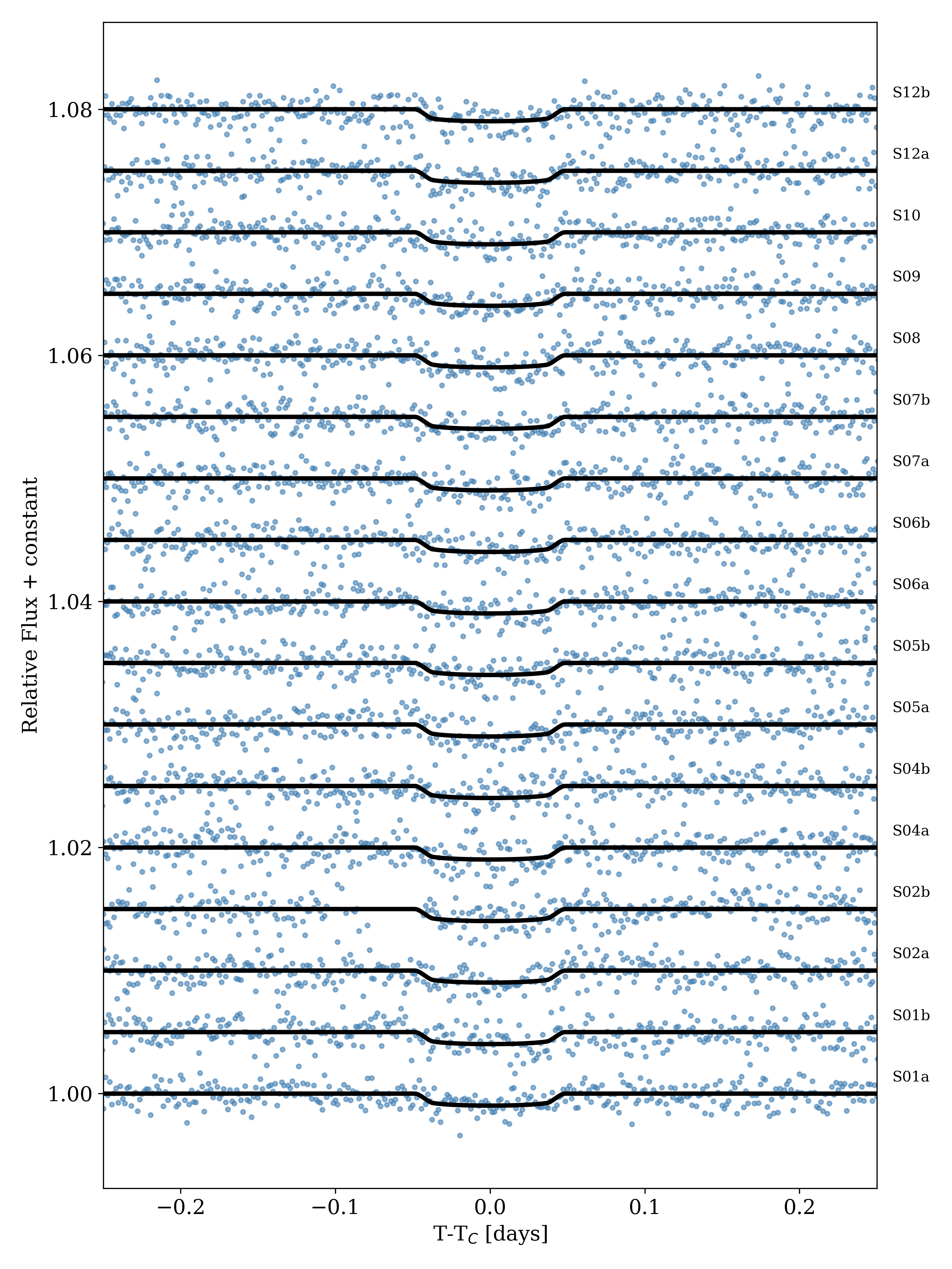
Figure 1: TOI-220 $b$ transit light curves extracted from the TESS data. The black solid line represents the best transit model (Sect. 3.3). The labels indicate the corresponding TESS sector.

Table 1: Summary of TOI-220 $b$ transits extracted from the TESS data.

TESS	transit mid-time	RMS(2 min)
Sector	[BJD_TDB]	[ppm]
S01	2458335.9024	890
S01	2458346.5976	941
S02	2458357.2928	897
S02	2458378.6832	903
S04	2458421.4640	979
S04	2458432.1592	909
S05	2458442.8544	942
S05	2458453.5496	949
S06	2458474.9400	952
S06	2458485.6352	882
S07	2458496.3304	908
S07	2458507.0257	929
S08	2458528.4161	924
S09	2458549.8065	911
S10	2458592.5873	833
S12	2458635.3681	961
S12	2458646.0633	938

2.2 HARPS follow-up

We obtained radial velocity measurements of TOI-220 with the HARPS spectrograph (Mayor et al., 2003) mounted on the 3.6 m telescope at ESO’s La Silla Observatory. HARPS is a stabilized high-resolution spectrograph with resolving power of R $\approx$ 115000, capable of sub m s^-1 RV precision. In total 101 observations were taken between 18 November 2018 and 11 October 2019 in high accuracy mode, of which 91 were used in the combined fit. Observations were performed under programmes 1102.C-0923 (PI: Gandolfi), 1102.C-0249 (PI: Armstrong), 0102.C-0584 (PI: De Medeiros), 60.A-9700 and 60.A-9709 (technical time). A typical exposure time of 1800 s was used, on occasion adjusted between 1500 s and 2100 s depending on sky condition and observing schedule. We achieved a typical signal-to-noise per pixel of 60 and an RV precision of 1.0 m s^-1.

Eight observations acquired on the nights between 25 and 27 November 2018 were excluded. On these dates the ThAr lamp used for wavelength calibration of HARPS was deteriorating and was subsequently exchanged on 28 November 2018. The changing flux ratio between the thorium and argon emission lines of the dying ThAr lamp induced a 2 m s${}^{-1}\,$d^-1 drift in the wavelength solution of the instrument over 5 d. The problematic data were confirmed by comparing unpublished data from the HARPS-N solar telescope (Dumusque et al., 2015; Collier Cameron et al., 2019) and those of the Helios program on HARPS, which also observes the Sun daily. Another observation done on the night of the 19 January 2019 was excluded due to an earthquake on that night. Finally, one observation on the night of the 17 April 2019 was excluded due to its very low signal-to-noise ratio. This gives 91 useful spectra.

The data were reduced with the HARPS data reduction software (DRS; Lovis & Pepe, 2007). Radial velocity measurements were derived using the weighted cross-correlation function (CCF) method using a K0 numerical mask (Pepe et al., 2002). For each spectrum, the DRS provides also the contrast, the full width at half maximum (FWHM), and the bisector inverse slope (BIS) of the cross-correlation function, as well as the Ca ii H & K lines activity indicator ($\log$ R${}^{\prime}_{\mathrm{HK}}$). We also extracted additional activity indexes and spectral diagnostics, namely, H$\alpha$, Na D, chromaticity (CRX), and differential line width (dLW), using the code SERVAL (Zechmeister et al., 2018). The 91 DRS and SERVAL RV measurements and activity indicators are listed in Tables 10 and 12. Time stamps are given in Barycentric Julian Dates in Barycentric Dynamical Time (BJD_TDB). The RV time series along with the best fitting model (Sect. 3.3) are shown in Fig. 7. We found an RV jitter below 2 m s^-1, consistent with the low activity level of the star (see Sect. 3.1 and 3.3).

2.3 High resolution imaging

To search for contaminating stars in the TESS photometric aperture, TOI-220 was observed on 9 January 2020 with the Zorro speckle instrument at Gemini South telescope. Zorro provides simultaneous speckle imaging in two bands, 562 nm and 832 nm, with output data products including a reconstructed image, and robust limits on companion detections (Howell et al., 2011). The contrast curve for the 832 nm is shown in Fig. 2. We also calculated from our high-resolution images the probability of contamination from blended and undetectable sources in the TESS aperture. We call this the blended source confidence (BSC) and the steps for estimating this probability are fully described in Lillo-Box et al. (2014). We used a python implementation of this technique (bsc, by J. Lillo-Box) which uses the trilegal galactic model (version 1.6; Girardi et al., 2012) to retrieve a simulated source population of the region around the corresponding target. From this simulated population, the density of stars around the target position (radius r=1^∘) was derived with the associated probability of chance-alignment at a given contrast magnitude and separation. We used the default parameters for the bulge, halo, thin/thick disks, and the lognormal initial mass function from Chabrier (2001). The Zorro contrast curve was then used to constrain this parameter space and estimate the final probability of undetected potentially contaminant sources. We considered as potentially contaminant sources those with a maximum contrast magnitude of $\Delta m_{\rm max}=-2.5\log{\delta}$, with $\delta$ being the transit depth of the candidate planet in the TESS band. This represents the maximum magnitude that a blended star can have to mimic this transit depth. We converted the depth in the TESS passband to the Zorro filters by using simple conversions using the TIC catalogue magnitudes and linking the 562 nm filter to the SDSSr band and the 832 nm filter to the SDSSz band. The corresponding conversions imply $\Delta m_{\rm 562\,nm}=0.954\Delta m_{\rm TESS}$ and $\Delta m_{\rm 832\,nm}=0.920\Delta m_{\rm TESS}$.

We applied this technique to TOI-220 using the two contrast curves available from the Gemini/Zorro instrument. The result provides a very low probability for an undetected source capable of mimicking the transit signal of 0.055 % for the 562 nm image and 0.015 % for the 832 nm image. We underline that using high-resolution images allowed us to significaly improve these probabilities by 26 % and 81 % for the 562 nm and 832 nm images, respectively, when comparing to the raw probabilities (i.e, without high-resolution images). As an example, we show in Fig. 2 the contrast curve and the results of the BSC analysis. In addition, by using the tpfplotter code (Aller et al., 2020) we ruled out the presence of contaminant sources within the TESS photometric aperture down to a $\Delta{\rm mag}=8$ mag in the Gaia DR2 catalogue (see Fig. 3).

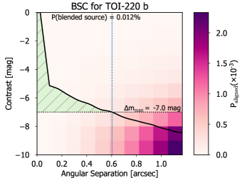
Figure 2: Contrast curve from the Gemini/Zorro instrument for the 832 nm filter (solid black line). The color on each angular separation and contrast bin represents the probability of a chance-aligned source with these properties at the location of the target, based on TRILEGAL model (see Sect. 2.3 within the main text). The maximum contrast of a blended binary capable of mimicking the planet transit depth is shown as a dotted horizontal line. The green-shaded region represents the non-explored regime by the high-spatial resolution image. The BSC corresponds to the integration of $P_{\rm aligned}$ over this shaded region.

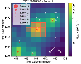
Figure 3: Target Pixel File of the TESS frame for TOI-220 corresponding to Sector 1 and computed with tpfplotter (Aller et al., 2020). The SPOC pipeline aperture is highlighted as red squares and the Gaia DR2 catalogue is over plotted with symbol sizes proportional to the magnitude contrast with the target.

2.4 Ground based photometric follow-up

We observed transit ingresses of TOI-220 $b$ in Pan-STARRS $z$-short band on 13 February 2019 and 21 December 2019 from the LCOGT (Brown et al., 2013) 1.0 m network node at South Africa Astronomical Observatory. We used the TESS Transit Finder, which is a customized version of the Tapir software package (Jensen, 2013), to schedule our transit observations. The $4096\times 4096$ LCOGT SINISTRO cameras have an image scale of 0.389$\arcsec$ per pixel, resulting in a $26\arcmin\times 26\arcmin$ field of view. The images were calibrated by the standard LCOGT banzai pipeline, and photometric data were extracted with AstroImageJ (Collins et al., 2017). The 13 February 2019 images were focused and have typical stellar point-spread-functions with a FWHM of $1\aas@@fstack{\prime\prime}9$, and circular apertures with radius $4\aas@@fstack{\prime\prime}3$ were used to extract the differential photometry. The 21 December 2019 images were defocused and have typical stellar point-spread-functions with a FWHM of $5\aas@@fstack{\prime\prime}2$, and circular apertures with radius $7\aas@@fstack{\prime\prime}8$ were used to extract the differential photometry. The light curves are presented in Appendix 14.

3 Data analysis

3.1 Stellar parameters

We derived the spectroscopic parameters and chemical abundance of TOI-220 from the co-added spectrum, which has an S/N per pixel at 5500 Å of $\sim$600. We used ares+moog, and followed the methodology described in Santos et al. (2013) and Sousa (2014) to derive the stellar atmospheric parameters (T_eff, $\log g$, microturbulence, [Fe/H]), and their respective uncertainties. We first measured equivalent widths (EW) of iron lines on the combined HARPS spectrum of TOI-220 using the ares v2 code (Sousa et al., 2015). Then we used a minimization process where we assume ionization and excitation equilibrium to converge in the best set of spectroscopic parameters. This process makes use of a grid of Kurucz model atmospheres (Kurucz, 1993) and the radiative transfer code MOOG (Sneden, 1973). Stellar abundances of the elements were derived using the classical curve-of-growth analysis method assuming local thermodynamic equilibrium (e.g. Adibekyan et al., 2012; Adibekyan et al., 2015; Delgado Mena et al., 2014; Delgado Mena et al., 2017). Abundances of the volatile elements, C and O, were derived following the method of Delgado Mena et al. (2010); Bertran de Lis et al. (2015). Since the two analysed spectral lines of oxygen (6158.17Å and 6300.3Å) are usually weak and the 6300.3Å line is blended with a Ni line (see e.g. Bertran de Lis et al., 2015), the EWs of these lines were manually measured with the task splot in IRAF. All the [X/H] ratios are obtained by doing a differential analysis with respect to a high S/N solar spectrum from HARPS, obtained from archival observations of the asteroid Vesta.

The stellar parameters and abundances of the elements are presented in Table 3. These results are in agreement with the values obtained from the Bayesian analysis described in Sect. 3.3. We found that the [X/Fe] ratios of $\alpha$ elements are slightly above solar. This fact together with a metallicity of -0.22 dex indicate that TOI-220 is probably an old star from the thin disk (e.g. Delgado Mena et al., 2019). Moreover, we used the chemical abundances of some elements to derive ages through the so-called chemical clocks (i.e. certain chemical abundance ratios which have a strong correlation for age). We applied the 3D formulas described in Table 10 of Delgado Mena et al. (2019), which also consider the variation in age produced by the effective temperature and iron abundance. We used the chemical clocks [Y/Mg], [Y/Zn], [Y/Ti], [Y/Si], [Y/Al], [Sr/Ti], [Sr/Mg] and [Sr/Si] from which we obtain a weighted average age of 10.1 $\pm$ 1.4 Gyr. This age is in agreement (within their uncertainties) with the age obtained from the Bayesian analysis described in the Sect. 3.3.

Following Johnson & Soderblom (1987) we calculated the space velocity components (UVW) with respect to the local standard of rest, adopting the standard solar motion (U_⊙, V_⊙, W_⊙) = (11.1, 12.24, 7.25) km s^-1 of Schönrich et al. (2010). Then, following Bensby et al. (2003) we calculated the probability of the star belonging to different stellar populations. For more details about the calculations of the kinematic properties of the stars see Adibekyan et al. (2012). Our calculations suggest that TOI-220 belongs to the galactic thin disk with a 98 % probability, in agreement with the chemical classification.

Finally, Canto Martins et al. (2020) studied TOI-220 in their recent study of 1000 TOIs and found no evidence of a coherent rotation period in the photometry, indicative of a low activity level. With a mean value of the Ca ii H & K lines activity index of $\log$ R${}^{\prime}_{\mathrm{HK}}$ = $-5.07\pm 0.05$, TOI-220 is magnetically less active than the Sun whose $\log$ R${}^{\prime}_{\mathrm{HK}}$ ranges from $-$4.86 to $-$4.95 from solar maximum to minimum (Hall et al., 2007).

3.2 Periodogram analysis of the HARPS measurements

We performed a frequency analysis of the HARPS RVs and spectral diagnostics to search for the Doppler reflex motion induced by TOI-220 $b$ and unveil the presence of additional signals that might be associated to stellar activity and/or arise from the orbital motion of other planets in the system.

The generalized Lomb-Scargle (GLS) periodogram (Zechmeister & Kürster, 2009) of the HARPS DRS RVs (Fig. 4, upper panel) shows a significant peak at f_b = 0.093 d^-1, i.e., the orbital frequency of the transiting planet detected in the TESS light curve. We estimated its false-alarm probability (FAP) using the bootstrap method described in Murdoch et al. (1993). Briefly, we computed the periodogram of 10⁶ mock time-series obtained by shuffling the RV measurements and their uncertainties, while keeping the time-stamps fixed. We defined the FAP as the fraction of those periodograms whose highest power exceeds the observed power of f_b in the periodogram of the original HARPS data at any frequency. We found no false positives out of our 10⁶ trials, implying that f_b has a FAP $<$ 10^-6. Moreover, the peak at f_b does not appear in any of the periodograms of the activity indicators (Fig. 4), confirming that the Doppler signal is induced by the presence of a bona fide planet, namely, TOI-220 $b$.

We subtracted the Doppler signal of the transiting planet TOI-220 b from the HARPS RVs by fitting a circular model,fixing the period and T₀ to the values derived from the modelling of the TESS light curves (with T₀ being equal to the mid-time of the first TESS transit), while allowing for the systemic velocity and RV semi-amplitude to vary. The GLS periodogram of the RV residuals displays significant (FAP $\,<\,$ 0.1 %) power at frequencies lower than $\sim$0.008 d^-1 (125 d), with a peak at about 0.0032 d^-1 (309 d) (Fig. 4, second panel). Despite this peak being undetected in the periodograms of the activity indicators and line asymmetry diagnostics (Fig. 4) – suggesting the presence of an additional outer companion – we note that its period is poorly constrained, being comparable to the temporal baseline of our observations (327 d). Moreover, the position of this peak depends on the last poorly-sampled measurements. Therefore, as discussed in Sect. 3.3.2, the exact nature of this long period signal can not be firmly constrained with the currently available RV data.

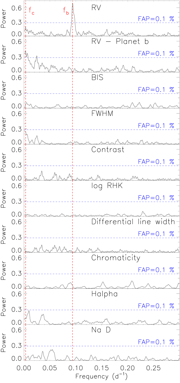
Figure 4: From top to bottom: Generalized Lomb-Scargle periodograms of the HARPS RV measurements (upper panel); the RV residuals following the subtraction of the signal of the transiting planet (second panel); the activity indicators of TOI-220 (remaining panels). The 0.1 % false alarm probability (FAP) estimated using the bootstrap method is shown with horizontal dashed lines. The vertical red lines mark the orbital frequencies the transiting planet TOI-220 $b$ (f_b = 0.093 d^-1) and of the additional Doppler signal we found in the HARPS RVs ($f_{\mathrm{c}}$ = 0.0032 d^-1).

3.3 PASTIS analysis

The Planet Analysis and Small Transit Investigation Software (Díaz et al., 2014; Santerne et al., 2015), pastis, was used for the joint analysis of the transit light curves, the radial velocities and the spectral energy distribution of TOI-220. The pastis package implements a fully Bayesian analysis of the data and uses the Markov Chain Monte Carlo (MCMC) method to sample the posterior distribution of the resulting parameters (see e.g. Santerne et al., 2019; Lopez et al., 2019, and references therein). We draw the posterior distributions of all free parameters after merging the best MCMC chains, i.e. those with the largest model likelihood ($\log$ L) from a sample of 30 chains with $10^{6}$ steps each. The convergence of these chains is checked by a Kologorov-Smirnov (K-S) test after the burn-in period (BI) of each chain has been removed. Here, the BI phase corresponds to the initial portion of each chain with a $\log$ L mean and variance 2 $\sigma$ away from the corresponding values of the last 10 % of the chain. Then, after removing the BI phase, the selected chains correspond to those with a median $\log$ L within 2 $\sigma$ of the best chain (i.e. the chain with the largest median $\log$ L) and with a K-S test p-value above 10^-30.

As mentioned in Sect. 2, 17 individual transits of TOI-220 $b$ were extracted from the TESS light curves and input to pastis. Additionally, a nightly binning was applied to the RV data in order to minimize the jitter induced by stellar activity and/or granulation, ending up thus with 69 points out of the total 91 RV measurements. The transits were modelled using jktebop software (Southworth, 2008) and the RV data using keplerian orbits.

3.3.1 Stellar SED analysis

pastis also models the host star by fitting the spectral energy distribution (SED) to the BT-Settl atmosphere models (Allard et al., 2012), Dartmouth evolutionary tracks (Dotter et al., 2008) and the quadratic limb darkening coefficients for TESS bandpass based on the tables from Claret & Bloemen (2011).

After a preliminary analysis using all the available magnitudes of TOI-220 (Table 2) we obtained a very poor fit of the visual magnitudes, in particular in the V band. We attributed this result to inconsistencies with the magnitude zero point used or with unreliable V magnitude estimations due to saturation of stars brighter than V=10 mag in the case of the APASS catalogue (Henden et al., 2015). As pastis does not implement the use of Gaia magnitudes by the time of this analysis, we decided to use only 2MASS (Skrutskie et al., 2006) and AllWISE (Cutri et al., 2013) magnitudes for the bayesian analysis. For this, we took TOI-220’s NIR magnitudes as reported in the TESS Input Catalogue (TICv8, Stassun et al., 2019). The host star was modelled for the effective temperature, T${}_{\text{eff}}$; surface gravity, $\log$ $g$; metallicity, [M/H]; distance, d; color excess, E(B$-$V); the systemic radial velocity, v₀, using as priors either normal or uniform distributions as presented in Table 6. The SED and best stellar model obtained with pastis are displayed in Fig. 5 and the fitted and derived stellar parameters are listed in Table 3. The resulting stellar parameters are consistent within their uncertainties with the values obtained independently from the spectral analysis described in Sect. 3.1.

Figure 5: Top panel: spectral energy distribution of TOI-220 with the best stellar atmosphere model from the BT-SETTL library obtained with pastis (blue solid line). Residuals are shown in the bottom panel (error bars include the fitted jitter from the analysis).

In order to corroborate the TOI-220’s effective temperature obtained with pastis and to discard any bias we could have introduced by using only NIR magnitudes, the observed and theoretical SEDs for TOI-220 were compared using the Virtual Observatory Spectral Analyzer (VOSA, Bayo et al., 2008). The observed SED was constructed using the four IR bands W1-W4 from allWISE, the J, H, and Ks bands from 2MASS (Skrutskie et al., 2006), and also including the 3 bands from Gaia (Gaia Collaboration et al., 2018). As before, the theoretical fluxes were computed from the grids of theoretical stellar spectra BT-Settl (AGSS2009, Allard et al., 2012). A best fit with the observed data was computed by $\chi^{2}$ minimization by testing effective temperature values ranging from 1000–7000 K with steps of 100 K. We also adopted the estimation of interstellar extinction provided in the TESS input catalog (Stassun et al., 2019), then computing the reddening according to Fitzpatrick (1999) and Schlafly & Finkbeiner (2011). The SED and the fitted stellar model are shown in Fig. 13. This independent analysis provides an effective temperature of 5300 $\pm$ 50 K, in very good agreement with the result from pastis. This analysis also shows no IR-excess, suggesting the absence of circumstellar material around TOI-220, at least in the WISE infrared bands.

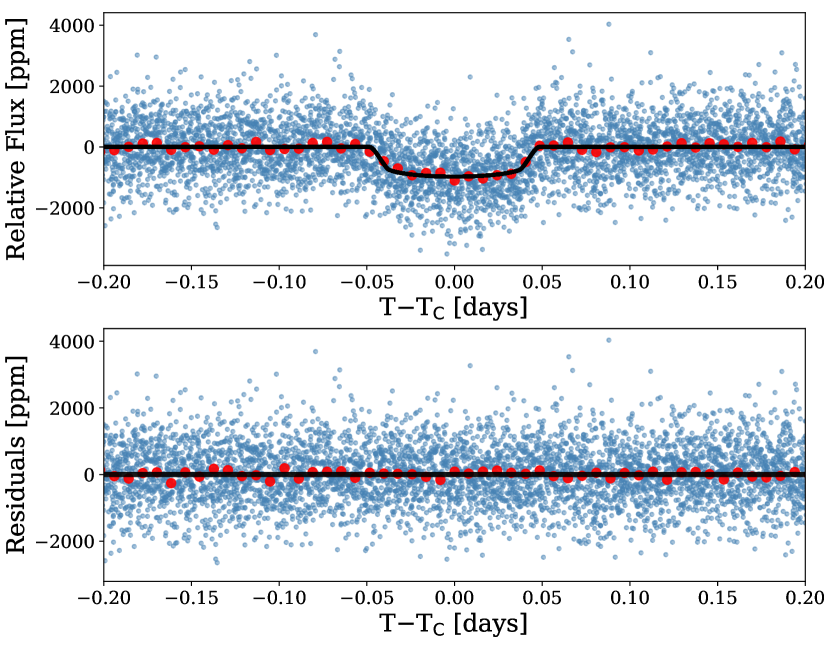
Figure 6: Top: TOI-220 $b$ transit light curve built by joining the 17 TESS transits used in this work (blue points and 12 min bins in red) together with the best model (solid curve) obtained with pastis analysis. The residuals are shown in the bottom panel.

3.3.2 Planetary analysis

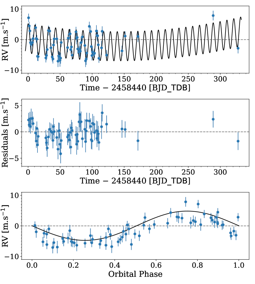
Figure 7: Radial velocity time series with the best fitted model superimposed with the corresponding residuals are shown in the top and middle panel, respectively. The phased radial velocity measurements are shown in the bottom panel. The error bars include the fitted jitter for each case. Additional, a fitted quadratic long-term is represented by a solid red curve in the middle pannel (see Sect 3.3.2 for details).

Based on the periodograms presented in Sect. 3.2, the data analysis of the TOI-220 system was performed taking into account the presence of a single planet in the system to probe the 10.69 d periodic signal. Additionally, we also included a quadratic, long-term RV trend in the modelling.

For the single planet scenario we modelled the planetary orbital period, P; the reference transit epoch, T₀; the star-planet radius ratio, $R_{\text{s}}/R_{\text{p}}$; the radial velocity semi-amplitude, K; and the inclination, eccentricity and argument of the periastron of the orbit: $i$, $e$ and $\omega$, respectively. The prior distribution used for each parameter is reported in Table 6. The posterior distribution of all the free parameters was drawn from the best 15 MCMC chains after removing the burn-in (BI) time (7–22 % of the chain). The full list of fitted and derived parameters of the system together with its respective 68.3 % confidence interval are given in Table 3 and 4 for the star and planet, respectively. Despite the good fit of the keplerian model, it seems that a structure is still present in the RV residuals (see e.g. Fig. 4, second panel). To better assess the significance of this trend, we applied the Anderson-Darling (A-D) test (Stephens, 1974) to the RV residuals (Table 7). The A-D test is a modification of the K-S test to evaluate whether a data sample comes from a specific distribution; in our case we tested the RV residuals against a Normal distribution. The test’s result is compared then to a set of critical values in a range of significance levels. In particular, the A-D test statistic (see Table 7) of the RV residuals is greater than the critical value at 15 % significance, 0.580 > 0.547 ($\alpha=0.15$), therefore the normality hypothesis of the RV residuals is rejected evidencing that they may contain astrophysical information not included in our single planet model.

Therefore, we also explored the effect of including a radial velocity quadratic trend in the RV modelling. For this, we used the same initial setup as before but adding two extra terms to account for a quadratic drift in the stellar radial velocity. We set a wide uniform distribution as a prior for the amplitude of the drift coefficients (Table 6). Here, we selected the best 20 MCMC chains after removing the BI (7–27 % of the chain) to draw the posterior distributions of the fitted parameters. The fitted drift coefficients are reported in Table 3 and the RV drift together with the 1-planet model are shown in Fig. 7. Despite the amplitude of the residuals being smaller when compared to the single planet scenario, the structure in the first epochs (t < 2458440.20 BJD) in the RV residuals seems to remain. But in this case, the normality of the residuals is not rejected by the A-D test. We show in Table 7 the result of this and other statistical tests which favour the inclusion of the RV drift in the modelling. Notably, the TOI-220 $b$ parameters are not affected by including this RV long term drift (Table 4). In Appendix E we show the mass constraints of a hypothetical second orbital body based on the estimated RV drift. Finally, we also checked the results when including a second planet in the modelling with a wide prior in the orbital period around the peak observed in the RV residual periodogram (300$\pm$100 d). We found that the RMS of the RV residuals are reduced, however, the resulting parameters for the second planet are poorly constrained. Based on this together with the fact that all the obtained parameters of TOI-220 $b$ remain fully compatible between models (see Table 4); and specially considering the baseline of the RV monitoring (only 327 d compared with the periodogram peak of the RV residuals of $\sim$309 d) and that the location of this peak strongly depends on the data points considered to calculate the periodogram; we adopt the values derived using the 1-planet with the quadratic RV long term drift shown in Tables 3 and 4 for the star and planet, respectively. We obtained for TOI-220 $b$ a planetary mass and radius of M${}_{\text{p}}$=13.8$\pm$1.0 M_⊕ and R${}_{\text{p}}$=3.03$\pm$0.15 R_⊕. The fitted orbital period and reference epoch are P=10.695264(86) d and T₀=2458335.9020(14) [BJD_TDB], respectively. The best model for each individual transit is shown in Fig. 1 and in Fig. 6 for the complete folded light curve of the 17 TESS transits. The best RV model including the RV quadratic drift and its residuals are displayed in Fig. 7. As a sanity check, we performed an independent joint analysis of the transit photometry and HARPS Doppler measurements using the code pyaneti (Barragán et al., 2019). We adopted the same PASTIS RV models and found consistent results well within the nominal error bars, corroborating the results of our analysis.

3.4 Transit Timing Variations

We performed the timing analysis of TOI-220 $b$ using the 17 TESS transits from sectors 1-12, the 4 transits of sectors 27-28; and the 2 transit observations obtained with the LCOGT telescopes. For this, we fixed all the transit parameters to the values obtained from pastis analysis in Sect. 3.3.2 except for the T${}_{\text{c}}$, R${}_{\text{p}}$/R${}_{\text{s}}$ and the inclination which were let free to vary. As the two LCOGT transits have a relative lower quality in terms of photometric precision and sampling; and owing to the fact that they cover only the ingress of the transit (see Fig. 14) we fixed also the inclination to i=87.88 $\deg$ for the modelling of these light curves. For the mid-times of the TESS transits, we used as priors a normal distribution with a 0.4 d width centred in the values obtained from the BLS analysis (Table 1). For each transit fit we used 20 MCMC chains of 10⁵ iterations. The obtained values for R${}_{\text{p}}$/R${}_{\text{s}}$ and inclination are consistent within the uncertainties in all the transits. The resulting transit mid-times are reported in Table 9. The average uncertainty of the transit mid-times is around 7 min. The first LCOGT transit has an uncertainty larger than 30 min in comparison with the 6 min of second LCOGT transit. As this light curve has a very poor photometric quality and transit coverage, we removed it from the analysis. With the obtained mid-times and the ephemeris equation:

$$\text{T}_{\text{c}}(n)=2458335.9021(14)[\text{BJD\_TBD}]+n\times 10.695264(86),$$ (1)

where P and T₀ are from Sect. 3.3.2; we estimated the timing residuals of TOI-220 $b$ as presented in Fig. 8 and Table 9. All the transit times are consistent within the uncertainties with a constant orbital period; the RMS of the O$-$C points is around 4.7 min. In addition, the statistical A-D test supports the hypothesis that the timing residuals are drawn from a normal distribution, discarding thus, orbital perturbations induced by a possible close companion.

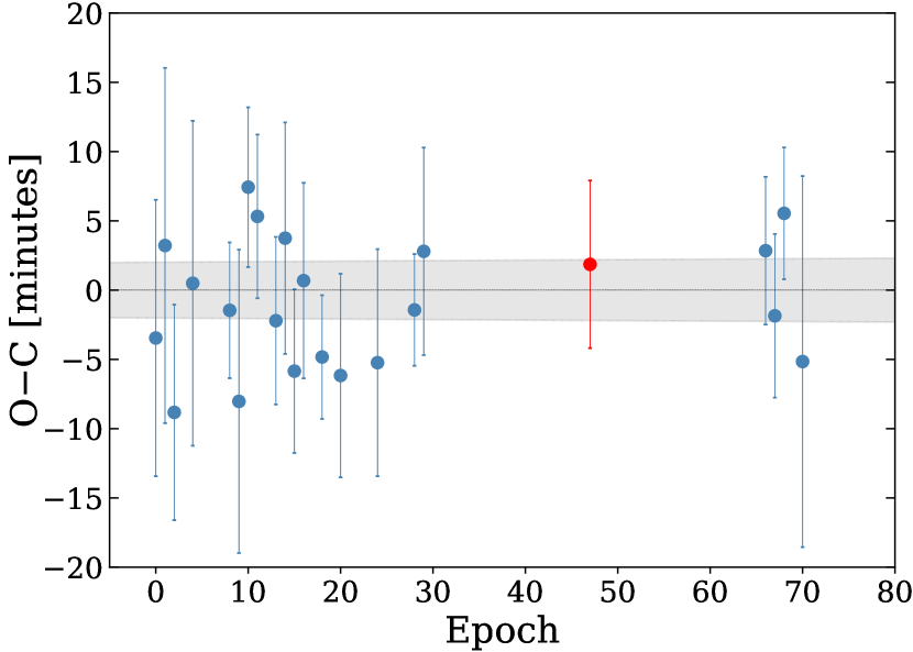
Figure 8: Observed minus Calculated diagram of the transit mid-times of TOI-220 $b$. Blue symbols correspond to TESS transits while the red symbol correspond to the second LCOGT transit observation. The shaded region represents the projected 1$\sigma$ uncertainties of ephemeris equation of TOI-220 $b$ (Sect. 3.4).

Table 2: TOI-220 main IDs, celestial coordinates and magnitudes.

Parameter	value	reference
TIC	150098860	(1)
TOI	220	(2)
TYC	8897-01263-1	(1)
APASS	29859752	(3)
2MASS	J06071197-6159487	(4)
WISE	J060711.93-615949.5	(5)
Gaia DR2	5481210874877547904	(6)
RA (J2000)	06:07:11.967	(1)
DEC (J2000)	-61:59:48.895	(1)
$\mu_{\text{RA}}$ [mas yr-1]	-17.815 $\pm$ 0.046	(6)
$\mu_{\text{DEC}}$ [mas yr-1]	-68.361 $\pm$ 0.042	(6)
Band	value	reference
TESS	$9.688\pm 0.006$	(1)
Johnson-V	$10.416\pm 0.263$	(3)
Johnson-B	$11.152\pm 0.032$	(3)
2MASS-J	$9.030\pm 0.024$	(4)
2MASS-H	$8.631\pm 0.031$	(4)
2MASS-Ks	$8.542\pm 0.025$	(4)
WISE-W1	$8.476\pm 0.023$	(5)
WISE-W2	$8.525\pm 0.020$	(5)
WISE-W3	$8.381\pm 0.021$	(5)
WISE-W4	$8.526\pm 0.167$	(5)
Gaia G	10.1897 $\pm$ 0.003	(6)
Gaia Bp	10.6078 $\pm$ 0.0012	(6)
Gaia Rp	9.6408 $\pm$ 0.0007	(6)
(1) TIC v8 (Stassun et al., 2019).
(2) TOI Catalogue (Guerrero et al. Submitted).
(3) AAVSO Photometric All-Sky Survey (Henden et al., 2015).
(4) Two Micron All Sky survey (Skrutskie et al., 2006).
(5) AllWISE Catalogue (Cutri et al., 2013).
(6) Gaia DR2 (Gaia Collaboration et al., 2018).

Table 3: Stellar properties of TOI-220.

Parameter	Value	Ref.
T${}_{\text{eff}}$ [K]	5273 $\pm$ 115	(1)
T${}_{\text{eff}}$ [K] (adopted)	5298 $\pm$ 65	(2)
T${}_{\text{eff}}$ [K]	$5384\pm 77$	(3)
T${}_{\text{eff}}$ [K]	$5182\pm 45$	(4)
$\log$ $g$ [cgs] (adopted)	4.37 $\pm$ 0.11	(2)
$\log$ $g$ [cgs]	4.25 $\pm$ 0.07	(4)
$\log$ $g$ [cgs]	4.49 $\pm$ 0.03	(3)
V${}_{\text{turb}}$ [km s-1]	0.694 $\pm$ 0.058	(2)
[Fe/H] [dex]	-0.217 $\pm$ 0.044	(2)
[M/H] [dex]	-0.19 $\pm$ 0.05	(3)
[Fe/H] [dex]	-0.2 $\pm$ 0.07	(4)
[Mg/H] [dex]	-0.10 $\pm$ 0.05	(2)
[Si/H] [dex]	-0.14 $\pm$ 0.04	(2)
[O/H] [dex]	-0.031 $\pm$ 0.072	(2)
[C/H] [dex]	-0.214 $\pm$ 0.045	(2)
[Cu/H] [dex]	-0.176 $\pm$ 0.044	(2)
[Zn/H] [dex]	-0.172 $\pm$ 0.027	(2)
[Sr/H] [dex]	-0.156 $\pm$ 0.077	(2)
[Y/H] [dex]	-0.293 $\pm$ 0.094	(2)
[Zr/H] [dex]	-0.236 $\pm$ 0.071	(2)
[Ba/H] [dex]	-0.237 $\pm$ 0.025	(2)
[Ce/H] [dex]	-0.166 $\pm$ 0.045	(2)
[Nd/H] [dex]	-0.100 $\pm$ 0.039	(2)
$v$ sin $i$ [km s-1]	2.90 $\pm$ 0.35	(4)
V${}_{\text{mac}}$ [km s-1]	0.9 $\pm$ 0.4	(4)
V${}_{\text{mic}}$ [km s-1]	0.85 $\pm$ 0.10	(4)
Age [Gyr] (adopted)	10.1 $\pm$ 1.4	(2)
Age [Gyr]	10.7${}^{+2.1}_{-3.1}$	(3)
Distance [pc]	89 $\pm$ 4	(3)
E(B$-$V) [mag]	0.163 $\pm$ 0.087	(3)
Systemic RV, v0 [m s-1]	26.45827 $\pm$ 0.00037	(3)
RV drift lin. coeff. [m s-1 d-1]	-0.0379(80)	(3)
RV drift quad. coeff. [m s-1 d-2]	0.000149(31)	(3)
Radius [R☉]	0.858 $\pm$ 0.032	(3)
Mass [M☉]	0.825 $\pm$ 0.028	(3)
Density [$\rho_{\sun}$]	1.31 $\pm$ 0.15	(3)
Limb darkening coeff. u${}_{\text{a}}^{\text{\tiny{TESS}}}$	0.352 $\pm$ 0.014	(3)
Limb darkening coeff. u${}_{\text{b}}^{\text{\tiny{TESS}}}$	0.2475 $\pm$ 0.0077	(3)
(1) TIC v8 (Stassun et al., 2019).
(2) From spectral analysis (Sect.3.1). Values correspond to weighted
average and the standard deviation.
(3) From pastis analysis (Sect. 3.3). Derived values assume
R☉=695 508 km and M☉= 1.98842 $\times$ 1030 kg.
(4) From spectral analysis validation (Appendix A)   .

Table 4: Results on the planetary parameters obtained from pastis simultaneous analysis of the data assuming a single planet system and by including a long term quadratic drift in the RVs. Derived values assume M_⊕ = 5.9736$\times$10²⁴ kg, R_⊕ = 6 378 137 m, AU = 149 597 870.7 km and zero albedo for the equilibrium temperature.

Parameter (fitted)	1 Planet	1 Planet + RV drift (adopted)
Orbital period, P [d]	10.695264(87)	10.695264(86)
Reference transit time, T0 [BJD$\_$TDB]	2458335.9021(14)	2458335.9020(14)
Planet-to-star radius ratio, R${}_{\text{p}}$/R${}_{\text{s}}$	0.03227 $\pm$ 0.00078	0.03235 $\pm$ 0.00076
Orbital inclination, $i$ [$\degr$]	$87.86\pm 0.14$	$87.88\pm 0.12$
RV semi-amplitude, K [m s-1]	4.47 $\pm$ 0.36	4.56 $\pm$ 0.32
Orbital eccentricity, $e$	$0.029^{\tiny{+0.034}}_{-0.021}$	$0.032^{+0.038}_{-0.023}$
Argument of periastron, $\omega$ [$\degr$]	159 $\pm$ 150	$248^{+66}_{-190}$
Parameter (derived)
Mass [M⊕]	$13.6\pm 1.2$	$13.8\pm 1.0$
Radius [R⊕]	$3.02\pm 0.17$	$3.03\pm 0.15$
bulk density, $\rho_{\text{p}}$ [g cm-3]	2.69 $\pm$ 0.55	2.73 $\pm$ 0.47
System scale, a/R${}_{\text{s}}$	22.3 $\pm$ 1.0	22.33 $\pm$ 0.80
Impact parameter, $b$	$0.832\pm 0.026$	$0.836\pm 0.022$
Transit duration, T14 [h]	2.231 $\pm$ 0.054	2.239 $\pm$ 0.055
orbital semi-major axis, a [AU]	0.08920 $\pm$ 0.0010	0.08911 $\pm$ 0.0010
Mean equilibrium temperature, T${}_{\text{eq}}$ [K]	806 $\pm$ 25	805 $\pm$ 21
Instrument-related parameters
HARPS jitter [m s-1]	1.71000 $\pm$ 0.00021	1.35000 $\pm$ 0.00024
SED jitter [mag]	0.048 $\pm$ 0.025	0.049 $\pm$ 0.026
TESS jitter [ppm]	111$\pm$74	111$\pm$ 74
TESS out-of-transit flux	1.000093(30)	1.000093(30)

4 Planetary Structure

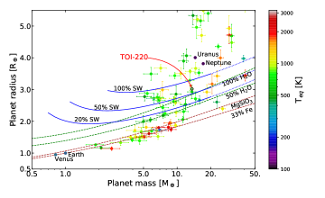
Figure 9: Mass-Radius diagram of the confirmed exoplanets with mass and radius measurements better than 20 % and 10 %, respectively. The symbol’s color scales with the equilibrium temperature of the planet. TOI-220 $b$ location in the diagram is highlighted with the red arrow and black circle. Solar System planets are also shown for reference. Composition models from Zeng et al. (2019) are displayed with dash brown and green lines. Those for a planet at 800 K with an Earth-like composition topped with various proportion of a steam and supercritical water layer (Mousis et al., 2020) are displayed with blue solid lines.

Table 5: Output parameters retrieved by the MCMC interior and atmosphere modeling.

Parameter	Value
Total mass, M${}_{\text{p}}$ [M⊕]	13.8$\pm$0.7
Total radius, R${}_{\text{p}}$ [R⊕]	3.06$\pm$0.12
Total density, $\rho_{\text{p}}$ [g cm-3]	2.65$\pm$0.28
Core mass fraction, CMF	0.08$\pm$0.03
Water mass fraction, WMF	0.62$\pm$0.10
Fe/Si mole ratio	0.64$\pm$0.11
Mg/Si mole ratio	1.16$\pm$0.10
Mg number, # Mg	0.85-1.0
Temperature at 300 bar, T${}_{\text{surf}}$ [K]	3536$\pm$203
Planetary albedo, $a_{\text{p}}$	0.230$\pm$0.001
Atmospheric thickness, z [km]	1111$\pm$99
Atmospheric mass, M${}_{\text{atm}}$ [M${}_{\oplus}\ 10^{-3}$]	1.31$\pm$0.16
Core+Mantle radius, [R${}_{\text{p}}$ units]	0.47$\pm$0.05

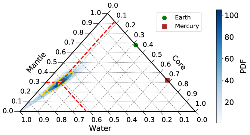
Figure 10: Sampled 2D marginal posterior distribution function for the CMF and WMF of TOI-220 $b$ (blue region). The PDF mean and the 1$\sigma$ confidence interval is marked by the yellow cross and curve, respectively. TOI-220 $b$ is consistent with a water rich planet (WMF=0.62$\pm$0.10) with a very small core (CMF=0.08$\pm$0.03). Earth and Mercury values are presented for comparison.

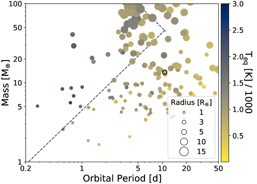
Figure 11: Mass-Period diagram of the confirmed exoplanets to date with masses and periods below 100 M_⊕ and 50 d, respectively (same planets sample as Fig. 9). The symbols size represents the radius of the planet while its equilibrium temperature is coded by the color of the symbol. TOI-220 $b$ is outlined with a black circle. The dashed lines mark the edges of the Neptune-desert from Mazeh et al. (2016).

Figure 9 shows the mass-radius diagram of all the confirmed exoplanets to date, with a precision better than 20 % and 10 % in their mass and radius, respectively. TOI-220 $b$ is well located in a domain of the sub-Neptune size planets. We investigate the interior of TOI-220 $b$ in order to get some insights into its composition. To that purpose we used the model of internal structure developed by Brugger et al. (2017) and recently updated by Mousis et al. (2020) to include a steam and supercritical water layer for the special case of highly-irradiated planets. When the pressure and temperature are above the critical point of water, water is in supercritical phase. To describe this water layer, we use the Equation of State (EOS) of Mazevet et al. (2019), which includes experimental and theoretical data of water at pressures and temperatures higher than the critical point of water. TOI-220 $b$ being strongly irradiated with an equilibrium temperature of 806 K, the model allows to address how its composition could differ from that of a Neptune-like planet with a large gaseous envelope overlying a rocky core. We followed the method described in Lillo-Box et al. (2020) and Acuña et al. (2021) exploring the core mass fraction (CMF, the ratio of the mass of the core and the total planetary mass) and the water mass fraction (WMF, the ratio of the mass of the water layer -steam and supercritical- and the total mass) of the planet as free parameters in an MCMC Bayesian framework adapted from Dorn et al. (2015).

We use as input parameters the planetary mass and radius, and the Fe/Si and Mg/Si mole ratios. The latter are calculated with the stellar abundances in Table 3 as Fe/Si = 0.65$\pm$0.09 and Mg/Si = 1.17$\pm$0.17. The code allows to explore the posterior distribution functions of three compositional parameters: CMF, WMF, and the Mg number ($\#$ Mg), which is a proxy for the level of differentiation of the planet as described by Sotin et al. (2007) and Brugger et al. (2017). If most of the Mg is located in the mantle and Fe in the core, the planet is highly differentiated and $\#$ Mg is close to one (0.9 for the case of Earth). On the contrary, if Mg and Fe are mixed in the mantle, $\#$ Mg will have lower values ($\simeq$ 0.6). In the MCMC algorithm, we assume uniform prior distributions of the CMF, WMF and the Mg number.

Table 5 shows the retrieved values of the three free compositional parameters, in addition to the observables (mass, radius and mole ratios), and the atmospheric variables. The posterior distributions of the CMF and WMF are also shown in Fig. 10. We used an MCMC algorithm to obtain samples of the posterior distribution of all our observable parameters: mass, radius, Fe/Si and Mg/Si. Convergence is achieved when the output parameters of the model reproduce the observed values within the 1$\sigma$ confidence intervals. Our results indicate that a planetary structure composed of a core rich in Fe, a silicate mantle and a supercritical water layer topped by a steam atmosphere in radiative-convective equilibrium is a likely scenario for TOI-220 $b$.

Since its host star is less enriched in Fe than the Sun and Earth (Fe/Si = 0.93), its CMF is significantly lower ($0.08\pm 0.03$) than the terrestrial value, 0.32. As can be seen in Table 5, the large $\#$ Mg obtained (0.85–1.0) is indicative of a highly-differentiated core and mantle configuration such as the Earth ($\#$ Mg=0.9). Furthermore, as shown in Fig. 10, TOI-220 $b$ could be a water-rich planet with a minimum WMF of 52%, which is compatible with the composition derived for water-rich satellites in the Solar System, such as Titan, and a maximum WMF of 72%, which is below the average water proportion found in comets (see Fig. 12 of McKay et al., 2019). Moreover, most of the water mass would be under pressure and temperature conditions beyond the supercritical point, forming a supercritical and steam water layer that would constitute 47% of the total radius.

5 Discussion

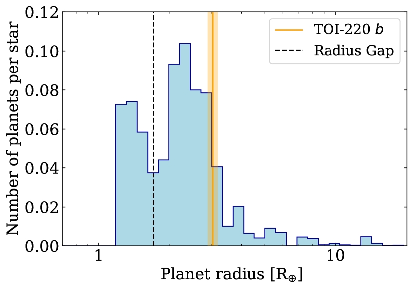
Figure 12: Histogram of the planetary radius for planets with periods below 100 d as presented in Fulton & Petigura (2018). The location of the radius gap and the size of TOI-220 $b$ ($\pm$1 $\sigma$) are shown with the black-dashed and orange-shaded lines, respectively.

The combined analysis of the photometric and spectroscopic data has fully confirmed the planetary nature of the TOI-220 $b$ transiting candidate. We noted the presence of a structure in the RV residuals on the exact nature of which, instrumental or planetary, we could not conclude with the data currently available. Therefore, any further investigation of the long-period signals would requires additional RVs. Thus, we adopt the values derived using a single planet model in the system and including a quadratic long term trend in the RVs. In Fig. 11 we show the mass-period diagram of all the confirmed exoplanets including TOI-220 $b$ (same sample as Fig. 9). The symbol size scales with the radii of planets while the color represents the planet’s equilibrium temperature. TOI-220 $b$ is located in the region of the warm sub-Neptunes class of exoplanets (T${}_{\text{eq}}$<1000 K) with a relatively large size (3 R_⊕).

A paucity of exoplanets has been reported in the planet size distribution around 1.5-2.0 R_⊕ (e.g. Fulton et al., 2017; Fulton & Petigura, 2018; Van Eylen et al., 2018), in particular for a M${}_{\star}\sim$ 0.8 M_☉ the gap is around 1.6 R_⊕. It is suggested that this gap is driven by photoevaporation mass-loss which acts shifting planets with gaseous envelopes towards a rocky Super-Earth population (R<1.7 R_⊕). TOI-220 $b$ lies above the gap in the Fulton’s diagram (see Fig. 12) in the not so populated high end of the size distribution of planets (R$\gtrsim$3 R_⊕) orbiting low mass stars (M_⋆<0.97 M_☉), as can be seen in Fig. 8 and 9 in Fulton & Petigura (2018). The atmospheric composition of TOI-220 $b$, either with a thick H/He layer or water rich content, suggests a formation in the protoplanetary disk past the snow line followed by slow migration. The host’s age of $\sim$10 Gyr points to a very evolved system and the large planet’s radius suggests the planet was massive enough to keep its atmosphere despite the large irradiation received by its host star. To get a first estimate of the atmospheric escape of TOI-220 $b$, we used equations of Aguichine et al. (Submitted). We found that the mass lost by Jeans’ escape is negilible even for light species (H/He) due to the surface gravity of the planet. Only $\sim$0.1 M_⊕ could be removed by XUV photo-evaporation along its 10.1 Gyr of life. This picture is consistent with the idea that the fate of warm sub-Neptunes located above the gap in the Fulton’s diagram (Fig. 12) is not to end their evolution as naked cores (see Deleuil et al., 2020; Bean et al., 2021, and references therein). Precise measurements of physical parameters of planets and its host stars, like the ones presented in this work, are key to shape the knowledge of the formation and evolution processes that sculpt the planet population in this region of parameter space.

Complementarily, we have performed an interior structure and atmosphere analysis within a Bayesian framework to constrain the composition of TOI-220 $b$ given its density and the stellar abundances of the host star. The low density of this strongly irradiated planet could be explained with a water-rich atmosphere that reaches the supercritical phase at its base, with a silicate mantle and an iron core as its bulk. As an alternative the planet might have a solid core surrounded by a thick H/He atmosphere. Future work should explore this possibility but also a composition with a well-mixed water and H/He atmosphere, since these are the most common volatiles that can form low-mass planets. The confirmation of the water-rich atmosphere scenario would also require conducting atmospheric characterisation to search for water spectral features. Following Kempton et al. (2018) we thus calculate TOI-220 $b$ transmission spectroscopy metric to check whether the planet would be amenable to such a characterization by JWST or the ELT. We obtained a value of 45, which is well below the threshold of 84 for planets in this range of size, making of TOI-220 $b$ atmosphere likely out of reach for the next decade.

6 Data Availability

The TESS photometric data used in this work is available via Mikulski Archive for Space Telescopes (MAST) archive and TFOP program. Radial velocity measurements and the derived stellar activity indicators are provided in Tables 10 and 12, respectively.

Appendix A Validation of stellar parameters

In addition to what has been presented in Sect. 3.1, as an independent validation, we also derived the main stellar parameters by applying the Spectroscopy Made Easy package (SME, Valenti & Piskunov, 1996; Piskunov & Valenti, 2017) to the co-added high signal-to-noise HARPS spectrum. SME uses grids of 1-D LTE stellar models to iteratively calculate synthetic spectra where by following a minimizing strategy each synthetic spectrum is compared to the normalized co-added spectrum observed data. The process is repeated by changing input parameters until we obtain a match for the line profiles of individual diagnostic lines, leading to values for T_eff, $\log$ $g$, metallicity, and $v$ sin $i$. The turbulent velocities are calculated according to the empirical relations of Bruntt et al. (2010) and Doyle et al. (2014) and are held fixed in the determination of the other parameters. We refer to Fridlund et al. (2020) for more details and references. With this, we found a slightly cooler T${}_{\text{eff}}$ = 5182 $\pm$ 45 K, while the rest of the calculated values $\log$ $g$ = 4.25 $\pm$ 0.07, Fe/H = $-$0.2 $\pm$ 0.07, $v$ sin $i$ = 2.9 $\pm$ 0.35 km s^-1, V_mic = 0.85 $\pm$ 0.1 km s^-1 (fixed) and V_mac = 0.9 $\pm$ 0.4 km s^-1, are in good agreement with the respective results of Sect. 3.1 presented in Table 3. Finally, the result of the independent SED fitting of TOI-220 described in Sect. 3.3.1 is shown in Fig. 13.

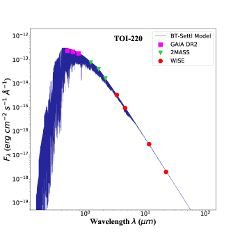
Figure 13: Independent SED fitting of TOI-220 using Gaia (magenta squares), 2MASS (green triangles) and WISE magnitudes (red circles). The blue solid line represents the fitted theoretical stellar model. See Sect.3.3 for details.

Appendix B Priors of the Bayesian analysis

In Table 6 we present the list of the prior distributions used for each parameter fitted with pastis code in Sect. 3.3.

Table 6: List of the prior distributions used in pastis analysis: $\mathcal{N}(\mu,\sigma^{2})$: Normal with mean $\mu$ and width $\sigma$; $\mathcal{U}(a,b)$: Uniform dist. between $a$ and $b$; $\mathcal{T}(\mu,\sigma^{2},a,b)$: Truncated normal distribution with mean $\mu$, width $\sigma$ between $a$ and $b$; and $\mathcal{S}(a,b)$: Sine dist. between $a$ and $b$. (*): parameters included in the RV drift modelling.

Stellar parameters	distribution
Effective Temperature, T${}_{\text{eff}}$ [K]	$\mathcal{N}(5300,100)$
Surface gravity, $\log$ $g$ [cgs]	$\mathcal{N}(4.5,0.1)$
Metallicity, [M/H] [dex]	$\mathcal{N}(-0.2,0.05)$
Distance, d [pc]	$\mathcal{N}(90.54,5)$
E(B$-$V) [mag]	$\mathcal{U}(0,1)$
Systemic RV, v0 [m s-1]	$\mathcal{U}(20,30)$
Reference Time RV [BJD_TDB] (*)	2458450
RV drift lin. coeff. [m s-1 d-1] (*)	$\mathcal{U}(-50,50)$
RV drift quad. coeff. [m s-1 d-2] (*)	$\mathcal{U}(-50,50)$
Planetary parameters
Orbital period, P [d]	$\mathcal{N}(10.6,0.5)$
Reference transit time, T0 [BJD_TDB]	$\mathcal{N}(2458335.9026,0.1)$
Planet-to-star radius ratio, R${}_{\text{p}}$/R${}_{\text{s}}$	$\mathcal{U}(0.029,0.04)$
RV semi-amplitude, K [m s-1]	$\mathcal{U}(0,10)$
Orbital inclination, $i$ [°]	$\mathcal{S}(85,90)$
Orbital eccentricity, $e$	$\mathcal{T}(0,0.32,0,1)$
Argument of periastron, $\omega$ [$\degr$]	$\mathcal{U}(0,360)$
Instrument parameters
TESS contamination [%]	$\mathcal{T}(0,0.005,0,1)$
TESS jitter [ppm]	$\mathcal{U}(0.0,0.1)$
TESS out-of-trasit flux	$\mathcal{U}(0.99,1.01)$
HARPS jitter [km s-1]	$\mathcal{U}(0.0,0.1)$
SED jitter [mag]	$\mathcal{U}(0,1)$

Appendix C Search for transits of planet-c in TESS light curve

As mentioned in Sect. 2, by the end of the writing of this manuscript two new sectors (27 and 28) from the second pass of TESS in the Southern hemisphere became available. These new data extend the photometric baseline for additional 43 days to the initial 311 days of the first sectors (after a gap of 395 days), allowing for a search of evidence of transits of additional planet in longer orbital periods. For this, we used the Box Least Squares (BLS) periodogram method over the TOI-220 full TESS light curve, i.e. the photometric time series containing the data of all the available sectors. We identified and masked the transits of TOI-220 $b$ at the orbital period of 10.69 d before conducting a wide search of transit-like features in a wide range of periods and durations adopting the minimun number of events in the light curve as two. It is worth mentioning that a photometric feature at BTJD$\sim$1417 was consistently identified as the first event by the BLS method. We confirmed that this event correspond to a known systematic spike reported in the TESS data release notes of the sector 4. After removing it, we found no significant peaks in the BLS. All the TESS light curves were also visually inspected searching for individual transits but only very low SNR features were identified. Therefore, there is no significant evidence of transits of an additional planet in the TESS data.

Appendix D Statistics and RV residuals of the 2 fitted models

In Table 7 we reported different statistical metrics we used to compare the models analyzed in Sect. 3.3.2: the single planet model with and without a radial velocity drift. We show the likelihood of each model and the $\Delta$AIC (which favours the inclusion of the RV drift) as well as the RMS of the radial velocity residuals and the Anderson-Darling test to check for the normality of the residuals. See detailed discussion in Sect. 3.3.2.

Table 7: Statistical comparison of the 2 models explored in this work.

Parameter	1 planet	1 planet + RV drift
$\log$ L	55474	55484
$\Delta$AIC	15	0
RV residuals RMS [m s-1]	1.93	1.69
A-D test	0.580	0.294
$\log$ L: log of the model likelihood.
AIC: Akaike information criterion.
A-D: Anderson-Darling test, to be compared with a critical value of
0.547, corresponding to a 15 % significance for normality rejection.

Appendix E Mass constraints of a hypothetical companion based on the RV drift

We note that the RV drift defined by the linear and quadratic coefficients of Table 3, which had been defined against the epoch of the first RV point (2458440.752469 BJD), can be replaced by a purely quadratic expression, given by $RV_{dr}=c_{2}(t-T_{0,dr})^{2}+k$, where $c_{2}$ is the quadratic coefficient of Table 3, $k$ is an offset without physical implications, and $T_{0,dr}$ defines the ’vertex’ of the parabolic function. With $c_{1}$ being the linear coefficient of the RV drift, the time of the vertex relative to the first RV-point is given by: $t_{v}=-c_{1}/(2c_{2})=127.18$ d, which results in an absolute value of $T_{0,dr}=2458567.933677$ BJD. This conversion permits us to describe the RV drift as a consequence of a hypothetical circular Keplerian orbit, with the drift given by:

$$y=-K\cos{\frac{2\pi t}{P}},$$ (2)

where $K$, $P$ and $t$ are the RV-amplitude, the period, and the time relative to $T_{0,dr}$. Considering that the second order Taylor expansion of $y=a\ \cos{bx}$ is given by $y=a-\frac{1}{2}x^{2}(ab^{2})+O(x^{4})$, the RVs of the Keplerian orbit can be approximated to second order by:

$$y^{\prime}=-K+[\frac{2\pi^{2}K}{P^{2}}]t^{2},$$ (3)

where the term in brackets corresponds now to the RV-drift’s quadratic coefficient of Table 3. Hence:

$$c_{2}=\frac{2\pi^{2}K}{P^{2}}=0.000149(31)\,[\text{m}\,\text{s}^{-1}\,\text{d}^{-2}]$$ (4)

For a given value of $P$, we may now solve this for $K$, and – using the stellar mass indicated in Table 3 – derive the mass of the hypothetical orbiter. This leads to the mass limits shown in Table 8. A lower limit of 750 days has been set, which is given by the validity of the Taylor approximation, which gets worse for shorter orbital periods. We note that only periods of less then $\approx$10000 d or 30 years lead to realistic masses, since longer periods correspond to stellar mass components that would have been detected by other means; e.g. through the SED of the target.

Table 8: Mass constraints based on the quadratic RV drift. $K$, $Kmin$ and $Kmax$ are the RV amplitudes corresponding to equation 4 solved for $K$, with the lower and upper errors set by the errors of $c_{2}$. M_pl is the orbiting object’s mass in units of Jupiter masses, based on the central $K$ value and a stellar mass of 0.828 M_☉.

P [d]	$K_{min}$ [m s-1]	$K$ [m s-1]	$K_{max}$ [m s-1]	Mpl [MJup]
750	3.36	4.25	5.13	0.17
1000	5.98	7.55	9.12	0.33
3000	53.80	67.94	82.07	4.25
10000	597.80	754.84	911.90	70.5
30000	5380.16	6793.59	8207.02	916

Appendix F Timing analysis of TOI-220 $b$

In Table 9 we reported the fitted transit time for each of the transits analyzed in Sect. 3.4. The transit ID is the same used in Table 1. The results of the two LCO transits (Fig. 14) are also shown. We reported the difference between these transit times and the estimated TOI-220 $b$ ephemeris equation (Eq. 1) which are presented in Fig. 8.

Transit ID	T${}_{\text{C}}$ [BJD_TBD]	+$\sigma$	-$\sigma$	O$-$C [min]
S01a	2458335.8997	0.0052	0.0083	-3.46
S01b	2458346.5996	0.0089	0.0089	3.22
S02a	2458357.2865	0.0054	0.0054	-8.82
S02b	2458378.6835	0.0057	0.0100	0.50
S04a	2458421.4632	0.0034	0.0034	-1.46
S04b	2458432.1539	0.0076	0.0076	-8.03
S05a	2458442.8599	0.0040	0.0040	7.43
S05b	2458453.5537	0.0041	0.0041	5.32
S06a	2458474.9390	0.0042	0.0042	-2.21
S06b	2458485.6384	0.0058	0.0058	3.75
S07a	2458496.3270	0.0041	0.0041	-5.85
S07b	2458507.0268	0.0049	0.0049	0.69
S08	2458528.4135	0.0031	0.0031	-4.83
S09	2458549.8031	0.0051	0.0051	-6.16
S10	2458592.5848	0.0066	0.0046	-5.24
S12a	2458635.3685	0.0028	0.0028	-1.43
S12b	2458646.0667	0.0052	0.0052	2.80
LCO1	2458528.420	0.024	0.024	4.53
LCO2	2458838.5808	0.0042	0.0042	1.86
S27a	2459041.7915	0.0037	0.0037	2.85
S27b	2459052.4835	0.0041	0.0041	-1.86
S28a	2459063.1839	0.0033	0.0033	5.54
S28b	2459084.5670	0.0093	0.0093	-5.16

Table 9: Transit mid-times obtained from individual fitting and their respective timing residuals (Sect. 3.4) using P=10.695264(87) d and T₀=2458335.9021(14) [BJD_TBD] (Sect.3.3.2).

Figure 14: Two transits of TOI-220 $b$ obtained with telescopes of the LCOGT network. The solid curves correspond to the fitted model of the timing analysis of the system (Sect 3.4) and are labelled with the corresponding ID of Table 9.

Appendix G Radial velocity data

In Tables 10 and 12 we report the radial velocity measurements together with the stellar activity indicators used in these work derived from the HARPS DRS and SERVAL, respectively (see Sect. 2.2).

Table 10: HARPS DRS radial velocity measurements and activity indicators of TOI-220. Exposure time and signal-to-noise ratio per pixel at 550 nm are given in the last two columns.

BJD_TDB	RV	$\sigma_{\text{RV}}$	BIS	FWHM	CCF	$\log$ R${}^{\prime}_{\mathrm{HK}}$	$\sigma_{\text{$\log$\,R${}^{\prime}_{\mathrm{HK}}$}}$	EXPTIME	SNR (550 nm)
$[$d]	[km s-1]	[km s-1]	[km s-1]	[km s-1]	CONTRAST			[s]	per pixel
2458440.708866	26.4650	0.0010	-0.0273	6.1504	40.3215	-5.0453	0.0102	1800	74.8
2458440.800232	26.4658	0.0010	-0.0233	6.1550	40.3239	-5.0352	0.0114	1800	73.4
2458441.758120	26.4637	0.0010	-0.0211	6.1550	40.2942	-5.0432	0.0111	1800	73.8
2458441.778259	26.4620	0.0009	-0.0253	6.1559	40.2737	-5.0481	0.0080	1800	83.0
2458442.807269	26.4601	0.0009	-0.0254	6.1487	40.3025	-5.0262	0.0104	1800	80.2
2458442.828449	26.4621	0.0010	-0.0260	6.1543	40.3186	-5.0557	0.0122	1800	79.9
2458443.686568	26.4573	0.0009	-0.0256	6.1541	40.2811	-5.0555	0.0101	1800	78.1
2458443.775781	26.4572	0.0010	-0.0267	6.1510	40.2879	-5.0614	0.0119	1800	71.4
2458444.809444	26.4567	0.0015	-0.0265	6.1551	40.2335	-5.0456	0.0181	1800	50.3
2458446.782081	26.4577	0.0008	-0.0211	6.1489	40.2909	-5.0626	0.0092	1800	90.4
2458446.830311	26.4568	0.0009	-0.0252	6.1547	40.2613	-5.0637	0.0111	1800	89.9
2458447.738845	26.4586	0.0008	-0.0237	6.1512	40.2769	-5.0318	0.0082	1800	87.4
2458447.834355	26.4585	0.0009	-0.0277	6.1535	40.2766	-5.0801	0.0114	1800	81.7
2458451.730670	26.4629	0.0008	-0.0270	6.1515	40.3034	-5.0619	0.0086	1800	92.5
2458451.805994	26.4611	0.0009	-0.0250	6.1557	40.2822	-5.0528	0.0118	1800	83.3
2458452.702375	26.4586	0.0008	-0.0249	6.1487	40.3235	-5.0401	0.0081	1500	88.2
2458452.782399	26.4587	0.0008	-0.0268	6.1491	40.3037	-5.0383	0.0098	1800	90.7
2458453.631164	26.4596	0.0009	-0.0255	6.1596	40.2811	-5.0500	0.0090	1800	83.5
2458453.773665	26.4572	0.0009	-0.0216	6.1523	40.3094	-5.0261	0.0093	1500	83.5
2458454.627488	26.4527	0.0012	-0.0228	6.1487	40.3376	-5.0787	0.0169	1500	61.2
2458454.750359	26.4528	0.0014	-0.0269	6.1542	40.2969	-5.0989	0.0200	1800	53.3
2458455.673973	26.4538	0.0012	-0.0219	6.1500	40.3438	-5.0740	0.0158	1500	60.4
2458455.790907	26.4516	0.0012	-0.0247	6.1566	40.3110	-5.0154	0.0146	1800	62.2
2458467.755644	26.4523	0.0009	-0.0251	6.1536	40.3024	-5.0391	0.0109	1500	80.6
2458468.701619	26.4530	0.0010	-0.0242	6.1563	40.3013	-5.0400	0.0101	1500	76.3
2458469.796343	26.4550	0.0012	-0.0271	6.1548	40.2970	-5.0806	0.0184	1500	65.4
2458471.743546	26.4612	0.0011	-0.0286	6.1537	40.3077	-5.0479	0.0144	1500	69.9
2458473.769591	26.4618	0.0008	-0.0210	6.1545	40.2550	-5.0396	0.0090	1800	91.0
2458473.790575	26.4602	0.0008	-0.0206	6.1549	40.2674	-5.0433	0.0103	1800	90.8
2458475.700867	26.4556	0.0010	-0.0263	6.1564	40.2620	-5.0359	0.0112	1500	75.3
2458477.683346	26.4526	0.0010	-0.0214	6.1553	40.2887	-5.0420	0.0107	1800	78.4
2458478.764436	26.4519	0.0010	-0.0224	6.1545	40.2691	-5.0313	0.0123	1800	81.5
2458479.671230	26.4565	0.0011	-0.0252	6.1502	40.2764	-5.0191	0.0115	1800	66.7
2458480.721428	26.4585	0.0008	-0.0259	6.1560	40.2723	-5.0374	0.0088	1800	90.2
2458484.774635	26.4585	0.0010	-0.0226	6.1556	40.2878	-4.9952	0.0122	1500	74.8
2458486.707656	26.4512	0.0015	-0.0257	6.1485	40.3665	-5.0866	0.0265	1500	52.9
2458487.719322	26.4529	0.0011	-0.0192	6.1580	40.2910	-5.0331	0.0144	1500	69.9
2458488.654032	26.4539	0.0012	-0.0229	6.1566	40.3144	-5.0545	0.0145	1500	60.1
2458488.794703	26.4516	0.0012	-0.0229	6.1561	40.3274	-5.0834	0.0222	1500	68.0
2458489.695779	26.4506	0.0025	-0.0164	6.1595	40.3359	-5.1050	0.0572	1500	34.6
2458489.817157	26.4522	0.0024	-0.0165	6.1478	40.3351	-5.2218	0.0715	1500	36.1
2458490.775790	26.4522	0.0014	-0.0237	6.1567	40.3240	-5.1718	0.0303	1500	58.0
2458491.667815	26.4571	0.0013	-0.0252	6.1522	40.2983	-4.9942	0.0147	1500	60.4
2458491.787386	26.4577	0.0017	-0.0199	6.1502	40.2760	-5.0854	0.0313	1500	48.0
2458501.597810	26.4573	0.0013	-0.0258	6.1493	40.2993	-5.0926	0.0183	1500	56.1
2458501.714141	26.4537	0.0014	-0.0271	6.1552	40.2865	-5.0426	0.0208	1500	54.5
2458502.585805	26.4593	0.0011	-0.0274	6.1552	40.2717	-5.0338	0.0130	1500	65.8
2458502.714208	26.4582	0.0011	-0.0206	6.1536	40.3083	-5.0889	0.0159	1500	73.2
2458504.675128	26.4600	0.0012	-0.0258	6.1602	40.2833	-5.0751	0.0170	1500	65.3
2458505.654443	26.4601	0.0010	-0.0212	6.1560	40.2635	-5.0220	0.0109	1500	72.6
2458506.564996	26.4558	0.0009	-0.0261	6.1547	40.2964	-5.0245	0.0083	1500	83.5
2458506.726419	26.4538	0.0011	-0.0222	6.1567	40.2421	-5.1025	0.0181	1500	75.1
2458507.570571	26.4557	0.0014	-0.0259	6.1586	40.3063	-5.0686	0.0203	1500	55.0
2458507.729911	26.4560	0.0014	-0.0248	6.1560	40.2585	-5.1037	0.0263	1500	58.5
2458508.653091	26.4533	0.0015	-0.0202	6.1525	40.3208	-5.0814	0.0274	1800	54.4
2458508.673450	26.4530	0.0015	-0.0162	6.1554	40.2769	-5.0783	0.0275	1800	55.3
2458514.784388	26.4608	0.0012	-0.0229	6.1629	40.2459	-5.0436	0.0185	1800	69.8
2458515.753041	26.4586	0.0016	-0.0213	6.1576	40.2386	-5.0440	0.0302	1240	50.8
2458516.577968	26.4592	0.0010	-0.0270	6.1551	40.3106	-5.0600	0.0126	1500	79.0
2458516.748836	26.4584	0.0015	-0.0263	6.1649	40.2796	-5.1390	0.0314	1500	55.9
2458517.578103	26.4552	0.0011	-0.0230	6.1566	40.3041	-5.0307	0.0140	1500	69.1
Continued

Table 11: continued

HARPS DRS radial velocity measurements and activity indicators of TOI-220. Exposure time and signal-to-noise ratio per pixel at 550 nm are given in the last two columns. BJD_TDB RV $\sigma_{\text{RV}}$ BIS FWHM CCF $\log$ R${}^{\prime}_{\mathrm{HK}}$ $\sigma_{\text{$\log$\,R${}^{\prime}_{\mathrm{HK}}$}}$ EXPTIME SNR (550 nm) $[$d] [km s^-1] [km s^-1] [km s^-1] [km s^-1] CONTRAST [s] per pixel 2458519.545756 26.4548 0.0015 -0.0236 6.1538 40.3182 -5.0835 0.0255 1500 52.5 2458519.730269 26.4523 0.0029 -0.0186 6.1508 40.2656 -5.2730 0.1117 1500 31.6 2458520.745206 26.4550 0.0021 -0.0245 6.1680 40.2821 -5.1150 0.0508 1500 41.5 2458521.549624 26.4544 0.0013 -0.0215 6.1534 40.3222 -5.0607 0.0192 1500 59.9 2458522.730498 26.4573 0.0016 -0.0215 6.1522 40.3176 -5.1530 0.0509 1500 55.9 2458524.738624 26.4591 0.0012 -0.0232 6.1538 40.3246 -5.0988 0.0283 1500 69.5 2458528.634749 26.4563 0.0015 -0.0292 6.1511 40.3093 -5.1221 0.0343 1500 53.7 2458529.725206 26.4513 0.0017 -0.0294 6.1658 40.1514 -4.9232 0.0266 1500 51.2 2458530.732839 26.4519 0.0016 -0.0271 6.1521 40.3033 -5.2255 0.0526 1500 54.9 2458531.549651 26.4538 0.0009 -0.0238 6.1536 40.3071 -5.0648 0.0120 1800 80.7 2458535.589291 26.4626 0.0010 -0.0252 6.1534 40.2066 -4.9657 0.0097 1800 79.7 2458537.672021 26.4609 0.0010 -0.0262 6.1585 40.2762 -5.0910 0.0222 1800 82.0 2458538.689271 26.4560 0.0013 -0.0312 6.1611 40.2935 -5.1449 0.0319 1800 66.9 2458539.678801 26.4530 0.0011 -0.0244 6.1564 40.2975 -5.0551 0.0220 1800 76.0 2458540.700230 26.4541 0.0014 -0.0254 6.1546 40.3270 -5.1352 0.0364 1800 63.8 2458542.669892 26.4534 0.0011 -0.0263 6.1511 40.3212 -5.1218 0.0237 1800 80.4 2458543.677293 26.4538 0.0010 -0.0270 6.1592 40.3075 -5.1119 0.0218 1800 89.6 2458546.690397 26.4611 0.0015 -0.0279 6.1612 40.3362 -5.1225 0.0379 1800 57.7 2458547.561096 26.4596 0.0012 -0.0283 6.1577 40.3057 -5.0859 0.0208 1800 70.5 2458548.556934 26.4595 0.0015 -0.0190 6.1614 40.2781 -5.0799 0.0259 1800 55.3 2458549.552540 26.4565 0.0009 -0.0240 6.1554 40.3031 -5.0554 0.0135 1800 88.0 2458550.576618 26.4521 0.0009 -0.0246 6.1621 40.2942 -5.0500 0.0152 1800 88.9 2458554.664806 26.4555 0.0020 -0.0280 6.1579 40.3187 -5.0843 0.0476 1800 44.5 2458555.650955 26.4610 0.0011 -0.0202 6.1623 40.3268 -5.1202 0.0256 1800 75.4 2458562.535601 26.4532 0.0012 -0.0251 6.1541 40.1392 -5.0067 0.0142 1800 69.5 2458586.560780 26.4545 0.0012 -0.0288 6.1560 40.3136 -5.0919 0.0252 1800 72.1 2458591.490221 26.4594 0.0010 -0.0267 6.1569 40.2479 -5.0704 0.0163 1800 84.4 2458611.494962 26.4593 0.0015 -0.0273 6.1592 40.2856 -5.0685 0.0292 1800 60.8 2458728.879893 26.4661 0.0011 -0.0235 6.1538 40.2937 -5.0360 0.0131 1800 76.9 2458767.767044 26.4554 0.0012 -0.0270 6.1482 40.1839 -5.0234 0.0118 2100 65.9

Table 12: HARPS SERVAL activity indicators of TOI-220.

BJD_TDB	dLW	$\sigma_{\text{dLW}}$	CRX	$\sigma_{\text{CRX}}$	H$\alpha$	$\sigma_{\text{H$\alpha$}}$	Na D	$\sigma_{\text{Na D}}$
$[$d]			[m s-1]	[m s-1]
2458440.708866	-0.2623	1.4290	-5.8768	11.5422	0.4656	0.0010	0.2665	0.0012
2458440.800232	-4.9625	1.5490	6.7761	11.0373	0.4668	0.0010	0.2670	0.0012
2458441.758120	-0.3565	1.3821	-1.7498	10.5452	0.4678	0.0011	0.2648	0.0012
2458441.778259	1.3307	1.1907	7.7788	9.8335	0.4675	0.0010	0.2669	0.0011
2458442.807269	-0.7192	1.3148	13.7782	9.0388	0.4691	0.0010	0.2604	0.0011
2458442.828449	-2.5532	1.2666	20.1963	9.1391	0.4644	0.0009	0.2596	0.0011
2458443.686568	2.2460	1.3634	-7.9982	10.3545	0.4654	0.0010	0.2678	0.0011
2458443.775781	2.9989	1.3117	-4.4235	11.2185	0.4667	0.0011	0.2664	0.0012
2458444.809444	3.6119	2.0043	2.4141	13.7423	0.4705	0.0016	0.2609	0.0018
2458446.782081	0.0413	1.0744	0.8902	9.4182	0.4691	0.0008	0.2610	0.0010
2458446.830311	3.3628	1.2715	-7.4150	10.0903	0.4681	0.0008	0.2610	0.0010
2458447.738845	0.6403	1.1213	0.1112	11.5124	0.4648	0.0009	0.2603	0.0010
2458447.834355	0.6680	1.4356	-2.1942	11.0709	0.4663	0.0009	0.2604	0.0011
2458451.730670	-0.0467	1.1565	6.0690	8.4936	0.4657	0.0008	0.2607	0.0009
2458451.805994	1.0959	1.3075	10.4416	9.3948	0.4649	0.0009	0.2611	0.0010
2458452.702375	-4.0832	1.2065	-13.0851	7.1234	0.4647	0.0009	0.2615	0.0010
2458452.782399	-2.7432	1.2199	-4.6426	6.7290	0.4642	0.0008	0.2597	0.0009
2458453.631164	-0.7047	1.0873	-2.9315	8.2828	0.4656	0.0009	0.2620	0.0011
2458453.773665	-1.1784	1.1849	-11.5157	8.6985	0.4646	0.0009	0.2622	0.0010
2458454.627488	-6.1300	1.7282	13.0497	9.5861	0.4664	0.0012	0.2596	0.0014
2458454.750359	-1.1140	2.5133	10.3401	13.2155	0.4679	0.0014	0.2617	0.0017
2458455.673973	-4.3860	1.6552	0.0656	9.5256	0.4649	0.0013	0.2591	0.0015
2458455.790907	-0.4042	1.7392	8.1142	10.3294	0.4678	0.0012	0.2686	0.0014
2458467.755644	0.0746	1.2988	0.2065	8.0561	0.4688	0.0009	0.2618	0.0011
2458468.701619	-1.4562	1.3661	11.2744	9.5247	0.4670	0.0010	0.2618	0.0012
2458469.796343	-1.7262	1.4104	-5.0228	10.2855	0.4640	0.0011	0.2618	0.0013
2458471.743546	-0.8041	1.4308	-4.8355	10.5433	0.4666	0.0011	0.2586	0.0012
2458473.769591	2.2120	0.9652	-11.8209	8.3775	0.4665	0.0008	0.2613	0.0010
2458473.790575	1.0648	1.2348	-21.6860	8.0858	0.4656	0.0008	0.2668	0.0009
2458475.700867	4.6992	1.3896	8.9426	9.7111	0.4637	0.0010	0.2592	0.0012
2458477.683346	1.4648	1.2915	7.2851	7.8859	0.4664	0.0010	0.2667	0.0011
2458478.764436	-0.6453	1.4899	-4.9377	8.2332	0.4655	0.0009	0.2686	0.0011
2458479.671230	-0.8130	1.7958	4.7311	10.6195	0.4703	0.0012	0.2661	0.0013
2458480.721428	2.7656	1.0797	-13.2663	8.3028	0.4663	0.0008	0.2659	0.0010
2458484.774635	0.3673	1.5322	0.8046	9.6450	0.4645	0.0010	0.2612	0.0012
2458486.707656	-3.1221	1.8534	-14.3388	11.9351	0.4633	0.0014	0.2587	0.0017
2458487.719322	1.1626	1.6061	8.9141	9.9225	0.4673	0.0011	0.2610	0.0013
2458488.654032	-2.4478	1.6747	5.4204	9.9891	0.4653	0.0013	0.2635	0.0015
2458488.794703	-3.6027	1.6175	-3.4279	8.9609	0.4658	0.0011	0.2627	0.0013
2458489.695779	-4.0812	3.2346	8.1978	20.4807	0.4661	0.0021	0.2585	0.0027
2458489.817157	1.4793	3.1791	35.1790	16.5534	0.4573	0.0020	0.2648	0.0026
2458490.775790	-1.9411	1.9919	7.9932	11.3483	0.4641	0.0012	0.2607	0.0015
2458491.667815	-1.8741	1.9072	-27.1674	10.1383	0.4719	0.0012	0.2612	0.0015
2458491.787386	-1.3321	2.4345	-0.3721	13.7161	0.4666	0.0015	0.2677	0.0018
2458501.597810	-2.3896	1.7019	-19.7716	12.1489	0.4692	0.0014	0.2673	0.0016
2458501.714141	0.0764	1.8841	-3.7394	10.5970	0.4663	0.0014	0.2596	0.0016
2458502.585805	-0.1945	1.7044	-6.8271	9.7077	0.4652	0.0012	0.2662	0.0013
2458502.714208	-1.9466	1.5951	-1.6920	8.8068	0.4656	0.0010	0.2603	0.0012
2458504.675128	-3.1907	1.5990	-9.1703	10.9906	0.4645	0.0012	0.2599	0.0014
2458505.654443	1.9881	1.5946	-6.0949	8.9858	0.4649	0.0011	0.2605	0.0012
2458506.564996	-0.4999	1.2270	-4.2423	8.2120	0.4657	0.0009	0.2584	0.0011
2458506.726419	2.2123	1.6614	-19.0888	9.1581	0.4646	0.0010	0.2610	0.0012
2458507.570571	-0.8163	2.1560	10.4649	15.1414	0.4643	0.0015	0.2610	0.0017
2458507.729911	4.2407	2.0254	-7.7070	10.3599	0.4634	0.0013	0.2596	0.0015
2458508.653091	0.6389	1.9808	35.3264	12.6350	0.4602	0.0014	0.2590	0.0017
2458508.673450	1.6420	1.9984	22.2776	14.2334	0.4580	0.0014	0.2585	0.0016
2458514.784388	7.0675	1.4771	-0.6879	10.9105	0.4560	0.0010	0.2667	0.0013
2458515.753041	8.4969	2.3699	-13.9389	13.3166	0.4573	0.0015	0.2661	0.0018
2458516.577968	-2.3914	1.5421	-24.5056	9.4269	0.4591	0.0010	0.2653	0.0011
2458516.748836	3.8234	2.0109	-4.3809	12.7091	0.4593	0.0014	0.2638	0.0016
2458517.578103	-2.6623	1.2879	-18.1996	9.1335	0.4581	0.0011	0.2682	0.0013
Continued

Table 13: continued

HARPS SERVAL activity indicators of TOI-220. BJD_TDB dLW $\sigma_{\text{dLW}}$ CRX $\sigma_{\text{CRX}}$ H$\alpha$ $\sigma_{\text{H$\alpha$}}$ Na D $\sigma_{\text{Na D}}$ $[$d] [m s^-1] [m s^-1] 2458519.545756 -2.7058 1.7916 -0.4067 11.4625 0.4669 0.0015 0.2652 0.0017 2458519.730269 2.1747 4.0675 -18.2779 19.2282 0.4634 0.0024 0.2696 0.0031 2458520.745206 1.2080 2.5333 -13.1655 15.8645 0.4589 0.0017 0.2636 0.0022 2458521.549624 -0.3015 1.6485 -5.2641 10.4197 0.4608 0.0013 0.2682 0.0015 2458522.730498 -0.9532 2.2842 27.7059 13.1662 0.4589 0.0013 0.2598 0.0016 2458524.738624 -1.2092 1.7960 -10.3374 11.4734 0.4593 0.0011 0.2622 0.0013 2458528.634749 -1.0433 1.9821 -8.1356 10.8765 0.4671 0.0014 0.2639 0.0017 2458529.725206 5.8613 2.6058 -5.5268 13.0208 0.4623 0.0015 0.2629 0.0018 2458530.732839 3.2712 2.0613 -26.2329 13.9351 0.4638 0.0014 0.2629 0.0016 2458531.549651 1.3428 1.2768 -6.5268 9.4249 0.4632 0.0010 0.2630 0.0011 2458535.589291 9.7591 1.3480 -3.8071 8.7267 0.4649 0.0010 0.2609 0.0011 2458537.672021 1.5254 1.2464 -3.3699 9.7638 0.4674 0.0009 0.2659 0.0011 2458538.689271 -0.6371 1.9865 15.3358 10.8076 0.4588 0.0012 0.2667 0.0013 2458539.678801 -0.8648 1.6380 -8.4122 10.2376 0.4589 0.0010 0.2644 0.0012 2458540.700230 -3.6376 1.8298 -11.8585 11.4789 0.4622 0.0012 0.2636 0.0014 2458542.669892 -2.4210 1.4654 6.2483 9.7577 0.4602 0.0010 0.2644 0.0011 2458543.677293 -1.3194 1.3547 -10.0779 10.2875 0.4590 0.0009 0.2672 0.0010 2458546.690397 -3.4933 2.0798 -16.0068 13.8284 0.4601 0.0013 0.2658 0.0016 2458547.561096 -2.6385 1.7150 18.2028 12.7411 0.4627 0.0011 0.2661 0.0013 2458548.556934 -1.0987 1.8158 6.1270 12.1296 0.4673 0.0015 0.2676 0.0017 2458549.552540 -0.2272 1.2355 -9.1661 8.6772 0.4652 0.0009 0.2668 0.0010 2458550.576618 -0.8848 1.3658 -3.7954 9.2115 0.4648 0.0009 0.2675 0.0010 2458554.664806 -1.0631 2.8411 26.3565 16.8388 0.4660 0.0018 0.2629 0.0021 2458555.650955 -2.6379 1.6708 -3.0134 12.1884 0.4660 0.0010 0.2617 0.0012 2458562.535601 11.6500 1.7232 2.8796 8.4236 0.4655 0.0012 0.2603 0.0013 2458586.560780 -2.4692 1.5497 1.8631 10.8953 0.4670 0.0011 0.2604 0.0012 2458591.490221 2.5875 1.5793 -6.1143 8.8415 0.4663 0.0010 0.2578 0.0010 2458611.494962 0.6165 2.0178 -8.6563 11.9310 0.4648 0.0013 0.2675 0.0015 2458728.879893 0.9451 1.7133 -8.4924 10.5144 0.4646 0.0011 0.2620 0.0012 2458767.767044 10.1703 1.7910 -0.4932 11.3817 0.4690 0.0013 0.2663 0.0014

Appendix H Affiliations

¹ Aix Marseille Univ, CNRS, CNES, LAM, Marseille, France.
² Dipartimento di Fisica, Universita degli Studi di Torino, via Pietro Giuria 1, I-10125, Torino, Italy.
³ Centre for Exoplanets and Habitability, University of Warwick, Gibbet Hill Road, Coventry, CV4 7AL, UK.
⁴ Department of Physics, University of Warwick, Gibbet Hill Road, Coventry CV4 7AL, UK.
⁵ Departamento de Física Teórica e Experimental, Universidade Federal do Rio Grande do Norte, Campus Universitário, Natal, RN, 59072-970, Brazil.
⁶ Centro de Astrobiología (CAB, CSIC-INTA), Depto. de Astrofísica, ESAC campus 28692 Villanueva de la Cañada (Madrid).
⁷ Instituto de Astrofísica e Ciências do Espaço, Universidade do Porto, CAUP, Rua das Estrelas, 4150-762 Porto, Portugal.
⁸ Departamento de Física e Astronomia, Faculdade de Ciências, Universidade do Porto, Rua do Campo Alegre, 4169-007 Porto, Portugal.
⁹ Leiden Observatory, Leiden University, 2333CA Leiden, The Netherlands.
¹⁰ Department of Space, Earth and Environment, Chalmers University of Technology, Onsala Space Observatory, 439 92 Onsala, Sweden.
¹¹ Center for Astrophysics | Harvard & Smithsonian, 60 Garden Street, Cambridge, MA 02138, USA.
¹² NASA Ames Research Center, Moffett Field, CA 94035, USA.
¹³ Instituto de Astrofísica de Canarias, 38205 La Laguna, Tenerife, Spain.
¹⁴ Departamento de Astrofísica, Universidad de La Laguna, 38206 La Laguna, Tenerife, Spain.
¹⁵ Sub-department of Astrophysics, Department of Physics, University of Oxford, Oxford, OX1 3RH, UK.
¹⁶ George Mason University, 4400 University Drive, Fairfax, VA, 22030 USA.
¹⁷ International Center for Advanced Studies (ICAS) and ICIFI (CONICET), ECyT-UNSAM, Campus Miguelete, 25 de Mayo y Francia, (1650) Buenos Aires, Argentina.
¹⁸ Thüringer Landessternwarte Tautenburg, Sternwarte 5, 07778 Tautenburg, Germany.
¹⁹ NASA Exoplanet Science Institute, Caltech/IPAC, Mail Code 100-22, 1200 E. California Blvd., Pasadena, CA 91125, USA.
²⁰ Dept. of Physics & Astronomy, Swarthmore College, Swarthmore PA 19081, USA.
²¹ U.S. Naval Observatory, 3450 Massachusetts Avenue NW, Washington, D.C. 20392, USA.
²² Observatoire de l’Université de Genève, Chemin des Maillettes 51, 1290 Versoix, Switzerland.
²³ University of Zürich, Institute for Computational Science, Winterthurerstrasse 190, 8057 Zürich, Switzerland
²⁴ European Southern Observatory, Alonso de Cordova 3107,Vitacura, Santiago, Chile.
²⁵ Department of Physics and Kavli Institute for Astrophysics and Space Research, Massachusetts Institute of Technology, Cambridge, MA 02139, USA
²⁶Department of Earth, Atmospheric and Planetary Sciences, Massachusetts Institute of Technology, Cambridge, MA 02139, USA
²⁷Department of Aeronautics and Astronautics, MIT, 77 Massachusetts Avenue, Cambridge, MA 02139, USA
²⁸ Hazelwood Observatory, Australia.
²⁹ Mullard Space Science Laboratory, University College London, Holmbury St. Mary, Dorking, Surrey, RH5 6NT, UK.
³⁰ Department of Astrophysical Sciences, Princeton University, 4 Ivy Lane, Princeton, NJ 08544, USA.
³¹ Univ. Grenoble Alpes, CNRS, IPAG, F-38000 Grenoble, France
³² Astrophysics Science Division, NASA Goddard Space Flight Center, Greenbelt, MD 20771, USA
³³ Deutsches Zentrum für Luft- und Raumfahrt, Institut für Planetenforschung, 12489 Berlin, Rutherfordstrasse 2., Germany.
³⁴ Center for Planetary Systems Habitability and McDonald Observatory, The University of Texas at Austin, Austin, TX 78730, USA.
³⁵ Noqsi Aerospace Ltd., 15 Blanchard Avenue, Billerica, MA 01821, USA
³⁶ Rheinisches Institut für Umweltforschung an der Universität zu Köln, Aachener Strasse 209, 50931 Köln, Germany.
³⁷ Astronomical Institute of the Czech Academy of Sciences, Fričova 298, Ondřejov 25168, Czech Republic
³⁸ Stellar Astrophysics Centre, Department of Physics and Astronomy, Aarhus University, Ny Munkegade 120,DK-8000 Aarhus C, Denmark
³⁹ Department of Astronomy, University of Tokyo, 7-3-1 Hongo, Bunkyo-ku, Tokyo 113-0033, Japan.
⁴⁰ Mikulski Archive for Space Telescopes.
⁴¹ NCCR/PlanetS, Centre for Space & Habitability, University of Bern, Bern, Switzerland.
⁴² Astronomy Department and Van Vleck Observatory, Wesleyan University, Middletown, CT 06459, USA
⁴³ SETI Institute, Mountain View, CA 94043, USA.
⁴⁴ Department of Astronomy, Columbia University, 550 W 120th Street, New York NY 10027, USA

References

- Acuña et al. (2021) Acuña L., Deleuil M., Mousis O., Marcq E., Levesque M., Aguichine A., 2021, A&A, 647, A53
- Adibekyan et al. (2012) Adibekyan V. Z., Sousa S. G., Santos N. C., Delgado Mena E., González Hernández J. I., Israelian G., Mayor M., Khachatryan G., 2012, A&A, 545, A32
- Adibekyan et al. (2015) Adibekyan V., et al., 2015, A&A, 583, A94
- Akeson et al. (2013) Akeson R. L., et al., 2013, PASP, 125, 989
- Allard et al. (2012) Allard F., Homeier D., Freytag B., 2012, Philosophical Transactions of the Royal Society of London Series A, 370, 2765
- Aller et al. (2020) Aller A., Lillo-Box J., Jones D., Miranda L. F., Barceló Forteza S., 2020, A&A, 635, A128
- Armstrong et al. (2020) Armstrong D. J., et al., 2020, Nature, 583, 39
- Astropy Collaboration et al. (2013) Astropy Collaboration et al., 2013, A&A, 558, A33
- Barragán et al. (2019) Barragán O., Gandolfi D., Antoniciello G., 2019, MNRAS, 482, 1017
- Bayo et al. (2008) Bayo A., Rodrigo C., Barrado Y Navascués D., Solano E., Gutiérrez R., Morales-Calderón M., Allard F., 2008, A&A, 492, 277
- Bean et al. (2021) Bean J. L., Raymond S. N., Owen J. E., 2021, Journal of Geophysical Research (Planets), 126, e06639
- Bensby et al. (2003) Bensby T., Feltzing S., Lundström I., 2003, A&A, 410, 527
- Bertran de Lis et al. (2015) Bertran de Lis S., Delgado Mena E., Adibekyan V. Z., Santos N. C., Sousa S. G., 2015, A&A, 576, A89
- Bhatti et al. (2020) Bhatti W., Bouma L., Joshua John Price-Whelan A., 2020, waqasbhatti/astrobase: astrobase v0.5.0, doi:10.5281/zenodo.3723832, https://doi.org/10.5281/zenodo.3723832
- Brown et al. (2013) Brown T. M., et al., 2013, Publications of the Astronomical Society of the Pacific, 125, 1031
- Brugger et al. (2017) Brugger B., Mousis O., Deleuil M., Deschamps F., 2017, ApJ, 850, 93
- Bruntt et al. (2010) Bruntt H., et al., 2010, A&A, 519, A51
- Canto Martins et al. (2020) Canto Martins B. L., et al., 2020, arXiv e-prints, p. arXiv:2007.03079
- Carleo et al. (2020) Carleo I., et al., 2020, arXiv e-prints, p. arXiv:2004.10095
- Chabrier (2001) Chabrier G., 2001, ApJ, 554, 1274
- Claret & Bloemen (2011) Claret A., Bloemen S., 2011, A&A, 529, A75
- Collier Cameron et al. (2019) Collier Cameron A., et al., 2019, MNRAS, 487, 1082
- Collins et al. (2017) Collins K. A., Kielkopf J. F., Stassun K. G., Hessman F. V., 2017, AJ, 153, 77
- Crossfield & Kreidberg (2017) Crossfield I. J. M., Kreidberg L., 2017, AJ, 154, 261
- Cutri et al. (2013) Cutri R. M., et al., 2013, Explanatory Supplement to the AllWISE Data Release Products, Explanatory Supplement to the AllWISE Data Release Products
- Deleuil et al. (2020) Deleuil M., Pollacco D., Baruteau C., Rauer H., Blanc M., 2020, Space Sci. Rev., 216, 105
- Delgado Mena et al. (2010) Delgado Mena E., Israelian G., González Hernández J. I., Bond J. C., Santos N. C., Udry S., Mayor M., 2010, ApJ, 725, 2349
- Delgado Mena et al. (2014) Delgado Mena E., et al., 2014, A&A, 562, A92
- Delgado Mena et al. (2017) Delgado Mena E., Tsantaki M., Adibekyan V. Z., Sousa S. G., Santos N. C., González Hernández J. I., Israelian G., 2017, A&A, 606, A94
- Delgado Mena et al. (2019) Delgado Mena E., et al., 2019, A&A, 624, A78
- Díaz et al. (2014) Díaz R. F., Almenara J. M., Santerne A., Moutou C., Lethuillier A., Deleuil M., 2014, MNRAS, 441, 983
- Dorn et al. (2015) Dorn C., Khan A., Heng K., Connolly J. A. D., Alibert Y., Benz W., Tackley P., 2015, A&A, 577, A83
- Dotter et al. (2008) Dotter A., Chaboyer B., Jevremović D., Kostov V., Baron E., Ferguson J. W., 2008, ApJS, 178, 89
- Doyle et al. (2014) Doyle A. P., Davies G. R., Smalley B., Chaplin W. J., Elsworth Y., 2014, MNRAS, 444, 3592
- Dumusque et al. (2015) Dumusque X., et al., 2015, ApJ, 814, L21
- Fitzpatrick (1999) Fitzpatrick E. L., 1999, PASP, 111, 63
- Fridlund et al. (2020) Fridlund M., et al., 2020, arXiv e-prints, p. arXiv:2008.12535
- Fulton & Petigura (2018) Fulton B. J., Petigura E. A., 2018, AJ, 156, 264
- Fulton et al. (2017) Fulton B. J., et al., 2017, AJ, 154, 109
- Gaia Collaboration et al. (2018) Gaia Collaboration et al., 2018, A&A, 616, A1
- Gandolfi et al. (2018) Gandolfi D., et al., 2018, A&A, 619, L10
- Gao et al. (2020) Gao P., et al., 2020, Nature Astronomy, 4, 951
- Ginzburg et al. (2018) Ginzburg S., Schlichting H. E., Sari R., 2018, MNRAS, 476, 759
- Girardi et al. (2012) Girardi L., et al., 2012, Astrophysics and Space Science Proceedings, 26, 165
- Gupta & Schlichting (2019) Gupta A., Schlichting H. E., 2019, MNRAS, 487, 24
- Hall et al. (2007) Hall J. C., Lockwood G. W., Skiff B. A., 2007, AJ, 133, 862
- Henden et al. (2015) Henden A. A., Levine S., Terrell D., Welch D. L., 2015, in American Astronomical Society Meeting Abstracts #225. p. 336.16
- Howell et al. (2011) Howell S. B., Everett M. E., Sherry W., Horch E., Ciardi D. R., 2011, AJ, 142, 19
- Hunter (2007) Hunter J. D., 2007, Computing in Science and Engineering, 9, 90
- Jenkins (2002) Jenkins J. M., 2002, ApJ, 575, 493
- Jenkins et al. (2010) Jenkins J. M., et al., 2010, in Software and Cyberinfrastructure for Astronomy. p. 77400D, doi:10.1117/12.856764
- Jenkins et al. (2016) Jenkins J. M., et al., 2016, in Proc. SPIE. p. 99133E, doi:10.1117/12.2233418
- Jenkins et al. (2020) Jenkins J. S., et al., 2020, Nature Astronomy, 4, 1148
- Jensen (2013) Jensen E., 2013, Tapir: A web interface for transit/eclipse observability, Astrophysics Source Code Library (ascl:1306.007)
- Johnson & Soderblom (1987) Johnson D. R. H., Soderblom D. R., 1987, AJ, 93, 864
- Jones et al. (2001) Jones E., Oliphant T., Peterson P., et al., 2001, SciPy: Open source scientific tools for Python, http://www.scipy.org/
- Kempton et al. (2018) Kempton E. M. R., et al., 2018, PASP, 130, 114401
- Kluyver et al. (2016) Kluyver T., et al., 2016, in Loizides F., Schmidt B., eds, Positioning and Power in Academic Publishing: Players, Agents and Agendas. pp 87 – 90
- Kurucz (1993) Kurucz R. L., 1993, VizieR Online Data Catalog, p. VI/39
- Li et al. (2019) Li J., Tenenbaum P., Twicken J. D., Burke C. J., Jenkins J. M., Quintana E. V., Rowe J. F., Seader S. E., 2019, PASP, 131, 024506
- Lillo-Box et al. (2014) Lillo-Box J., Barrado D., Bouy H., 2014, A&A, 566, A103
- Lillo-Box et al. (2020) Lillo-Box J., et al., 2020, A&A, 640, A48
- Lopez et al. (2019) Lopez T. A., et al., 2019, A&A, 631, A90
- Lovis & Pepe (2007) Lovis C., Pepe F., 2007, A&A, 468, 1115
- Mayor et al. (2003) Mayor M., et al., 2003, The Messenger, 114, 20
- Mazeh et al. (2016) Mazeh T., Holczer T., Faigler S., 2016, A&A, 589, A75
- Mazevet et al. (2019) Mazevet S., Licari A., Chabrier G., Potekhin A. Y., 2019, A&A, 621, A128
- McKay et al. (2019) McKay A. J., et al., 2019, AJ, 158, 128
- McKinney (2010) McKinney W., 2010, in van der Walt S., Millman J., eds, Proceedings of the 9th Python in Science Conference. pp 51 – 56
- Morley et al. (2015) Morley C. V., Fortney J. J., Marley M. S., Zahnle K., Line M., Kempton E., Lewis N., Cahoy K., 2015, ApJ, 815, 110
- Mousis et al. (2020) Mousis O., Deleuil M., Aguichine A., Marcq E., Naar J., Aguirre L. A., Brugger B., Gonçalves T., 2020, The Astrophysical Journal, 896, L22
- Murdoch et al. (1993) Murdoch K. A., Hearnshaw J. B., Clark M., 1993, ApJ, 413, 349
- Nielsen et al. (2020) Nielsen L. D., et al., 2020, MNRAS, 492, 5399
- Owen & Lai (2018) Owen J. E., Lai D., 2018, MNRAS, 479, 5012
- Pandas development team. (2020) Pandas development team. 2020, pandas-dev/pandas: Pandas, doi:10.5281/zenodo.3509134, https://doi.org/10.5281/zenodo.3509134
- Pepe et al. (2002) Pepe F., et al., 2002, The Messenger, 110, 9
- Pérez & Granger (2007) Pérez F., Granger B. E., 2007, Computing in Science and Engineering, 9, 21
- Piskunov & Valenti (2017) Piskunov N., Valenti J. A., 2017, A&A, 597, A16
- Price-Whelan et al. (2018) Price-Whelan A. M., et al., 2018, AJ, 156, 123
- Ricker et al. (2015) Ricker G. R., et al., 2015, Journal of Astronomical Telescopes, Instruments, and Systems, 1, 014003
- Santerne et al. (2015) Santerne A., et al., 2015, MNRAS, 451, 2337
- Santerne et al. (2019) Santerne A., et al., 2019, arXiv e-prints, p. arXiv:1911.07355
- Santos et al. (2013) Santos N. C., et al., 2013, A&A, 556, A150
- Schlafly & Finkbeiner (2011) Schlafly E. F., Finkbeiner D. P., 2011, ApJ, 737, 103
- Schönrich et al. (2010) Schönrich R., Binney J., Dehnen W., 2010, MNRAS, 403, 1829
- Skrutskie et al. (2006) Skrutskie M. F., et al., 2006, AJ, 131, 1163
- Smith et al. (2012) Smith J. C., et al., 2012, PASP, 124, 1000
- Sneden (1973) Sneden C. A., 1973, PhD thesis, THE UNIVERSITY OF TEXAS AT AUSTIN.
- Sotin et al. (2007) Sotin C., Grasset O., Mocquet A., 2007, Icarus, 191, 337
- Sousa (2014) Sousa S. G., 2014, [arXiv:1407.5817],
- Sousa et al. (2015) Sousa S. G., Santos N. C., Adibekyan V., Delgado-Mena E., Israelian G., 2015, A&A, 577, A67
- Southworth (2008) Southworth J., 2008, MNRAS, 386, 1644
- Stassun et al. (2019) Stassun K. G., et al., 2019, AJ, 158, 138
- Stephens (1974) Stephens M. A., 1974, Journal of the American Statistical Association, 69, 730
- Stumpe et al. (2012) Stumpe M. C., et al., 2012, PASP, 124, 985
- Stumpe et al. (2014) Stumpe M. C., Smith J. C., Catanzarite J. H., Van Cleve J. E., Jenkins J. M., Twicken J. D., Girouard F. R., 2014, PASP, 126, 100
- Szabó & Kiss (2011) Szabó G. M., Kiss L. L., 2011, ApJ, 727, L44
- Twicken et al. (2018) Twicken J. D., et al., 2018, PASP, 130, 064502
- Valenti & Piskunov (1996) Valenti J. A., Piskunov N., 1996, A&AS, 118, 595
- Van Der Walt et al. (2011) Van Der Walt S., Colbert S. C., Varoquaux G., 2011, preprint, (arXiv:1102.1523)
- Van Eylen et al. (2018) Van Eylen V., Agentoft C., Lundkvist M. S., Kjeldsen H., Owen J. E., Fulton B. J., Petigura E., Snellen I., 2018, MNRAS, 479, 4786
- West et al. (2019) West R. G., et al., 2019, MNRAS, 486, 5094
- Zechmeister & Kürster (2009) Zechmeister M., Kürster M., 2009, A&A, 496, 577
- Zechmeister et al. (2018) Zechmeister M., et al., 2018, A&A, 609, A12
- Zeng et al. (2019) Zeng L., et al., 2019, Proceedings of the National Academy of Science, 116, 9723