NANOGrav signal and LIGO-Virgo Primordial Black Holes from the Higgs field
Abstract
We show that the NANOGrav signal can come from the Higgs field with a noncanonical kinetic term in terms of the scalar induced gravitational waves. The scalar induced gravitational waves generated in our model are also detectable by space-based gravitational wave observatories. Primordial black holes with stellar masses that can explain LIGO-Virgo events are also produced. Therefore, the NANOGrav signal and the BHs in LIGO-Virgo events may both originate from the Higgs field.
1 Introduction
The North American Nanohertz Observatory for Gravitational Wave (NANOGrav) Collaboration has recently published an analysis of the yrs pulsar timing array (PTA) data, where strong evidence of a stochastic process with a common amplitude and a common spectral slope across pulsars was found [1]. Although this process lacks quadrupolar spatial correlations, which should exist for gravitational wave (GW) signals, it is worthwhile to be interpreted as a stochastic GW signal. The GW signal with the amplitude of the energy density at a reference frequency of Hz has a flat power spectrum with from to at confidence level.
The scalar induced gravitational waves (SIGWs) associated with the formation of primordial black holes (PBHs) are the natural sources to explain the NANOGrav signal [2, 3, 4, 5, 6, 7, 8]. (For other explanations for the sources of the NANOGrav signal, see Ref. [9, 10, 11, 12, 13, 14, 15, 16, 17, 18, 19, 20, 21, 22, 23, 24].) The nanohertz frequencies of SIGWs constrain the masses of PBHs to stellar mass, and these stellar mass PBHs, on the other hand, may be the sources of the GWs detected by the Laser Interferometer Gravitational Wave Observatory (LIGO) Scientific Collaboration and the Virgo Collaboration [25, 26, 27, 28, 29, 30, 31, 32, 33, 34, 35, 36, 37, 38]. Therefore, PBHs with stellar mass can be related to both the LIGO-Virgo events and the NANOGrav signal. The PBHs are also proposed to account for the dark matter (DM) [39, 40, 41, 42, 43, 44, 45, 46, 47, 48, 49, 50] and explain the Planet 9 which is a hypothetical astrophysical object in the outer solar system used to interpret the anomalous orbits of trans-Neptunian objects [51].
PBHs will be formed from the gravitational collapse if the density contrasts of overdense regions exceed the threshold value at the horizon reentry during radiation domination [52, 53]. The initial conditions for the overdense regions are from the inflation. Enough abundance of PBHs needs the amplitude of the power spectrum of the primordial curvature perturbations reach at small scales, and this condition is also required to explain the NANOGrav signal if it is regarded as a SIGW. The constraint on the amplitude of the power spectrum at large scales from the cosmic microwave background (CMB) anisotropy measurements is [54]. Therefore, to produce enough abundance of PBH DM, the amplitude of the power spectrum should be enhanced at least seven orders of magnitude to reach the threshold at small scales [55, 56, 57].
The traditional slow-roll inflation is unable to enhance the power spectrum to produce PBHs while keeping the model consistent with the CMB constraints. To overcome this, the ultra-slow-roll inflation [58, 59, 60] is then considered [61, 62, 63, 64, 55, 65, 66, 67, 68, 69, 70, 71, 72, 73, 74, 75, 76, 77]. Among them, the inflation model with a noncanonical kinetic term can successfully enhance the power spectra, produce PBHs, and generate SIGWs [78, 79, 80]. In this mechanism, there are no restrictions on the potential, both sharp and broad peaks in the power spectrum can be generate, the masses of the PBHs and the frequencies of the SIGWs can be adjusted as we want. Although any potential can be applied in this mechanism, the most natural potential to drive the inflation may be the Higgs field, as it is the only scalar field in the standard model of particle physics and has been detected by the Large Hadron Collider [81, 82, 83]. In this paper, we will show that under this mechanism, the NANOGrav signal and the BHs in the LIGO-Virgo events can both come from the Higgs field.
The paper is organized as follows. In Sec. 2, we give a brief review of the PBHs and SIGWs. We introduce our model and produce PBHs with stellar mass and generate SIGWs consistent with the NANOGrav signal in Sec. 3, We conclude the paper in Sec. 4.
2 The PBHs and scalar induced GWs
If the energy density contrast of overdensity regions is large enough during the radiation domination, the PBHs will be formed from gravitational collapse, and the seed of the overdensity regions is from the primordial curvature perturbations generated during inflation. The mass fraction of the Universe that collapses to form PBHs at formation is
| (2.1) |
where is the energy density of the background and is the energy density of the PBHs at formation, which can be obtained by the peak theory[84, 85, 86, 87, 88, 89],
| (2.2) |
where the number density of the PBHs at formation is
| (2.3) |
and is the threshold for the formation of PBHs, is the variance of the smoothed density contrast and is the moment of the smoothed density power spectrum with the definition,
| (2.4) |
The relation between the power spectrum of the density contrast and the power spectrum of primordial curvature perturbations is
| (2.5) |
with the state equation during the radiation domination. The window function we choose in this paper is the real space top-hat window function
| (2.6) |
with the smoothed scale . The threshold is dependent on the choice of the window function and the shape of the density perturbation [88, 90, 87]. For the real space top-hat window function, we choose the threshold as [91, 90]. During radiation domination with constant degrees of freedom, the transfer function is
| (2.7) |
The masses of the PBHs obey the critical scaling law [92, 93, 94],
| (2.8) |
with for the real space top-hat window function and in the radiation domination [92, 93]. The horizon mass related to the horizon scale is
| (2.9) |
where is the number of relativistic degrees of freedom at the formation. The density parameter of the PBHs expressed by the is [95]
| (2.10) |
where we use the relation and during radiation domination, and is the horizon mass at the matter-radiation equality. Because of at the condition or , for the sake of simplicity, we choose the interval of the integration as and . The fraction of the PBHs in the dark matter is
| (2.11) |
where the definition of the PBHs mass function is
| (2.12) |
Combining Eq. (2.10) and Eq. (2.12) and using the relation (2.8), the mass function becomes [95]
| (2.13) |
where and we have used .
Associating with the formation of PBHs, the large scalar perturbations induce the gravitational waves during radiation domination. These SIGWs belonging to the stochastic background can account for the NANOGrav signal with frequencies around Hz [4, 2, 3] and can also be detected by the space-based GW detectors like LISA [96, 97], Taiji [98] and TianQin [99] with frequencies around Hz in the future. In the cosmological background and the Newtonian gauge and neglecting the anisotropic stress, the perturbed metric is
| (2.14) |
where is the conformal time, is the Bardeen potential. In the Fourier space, the tensor perturbations can be expressed as
| (2.15) |
where and are the plus and cross polarization tensors,
| (2.16) | |||
| (2.17) |
with . Focusing on the source at second order from the linear scalar perturbations, the tensor perturbations in the Fourier space with either polarization satisfy [100, 101]
| (2.18) |
where a prime denotes the derivative with respect to the conformal time, , and is the conformal Hubble parameter. The second order source from the linear scalar perturbations is
| (2.19) |
where is Bardeen potential in Fourier space, and related to the primordial curvature perturbation by the transfer function,
| (2.20) |
The power spectrum for the SIGWs is
| (2.21) |
which is found to be [101, 100, 102, 103]
| (2.22) |
where , , and the integral kernel is
| (2.23) |
The energy density of the SIGWs is [103, 56]
| (2.24) |
where is the oscillation time average of the integral kernel. After formation, the SIGWs behave like radiation, so the energy density of the SIGWs at present is
| (2.25) |
where is the energy density of radiation at present, and [4, 2]
| (2.26) |
3 The model and results
To obtain enough abundance of PBH DM and induce secondary GWs with large energy density, the amplitude of the power spectrum of the primordial curvature perturbations should be enhanced about seven order of magnitude at small scales. In this section, we present our model and show that the PBHs that account for LIGO-Virgo events and the SIGWs which are consistent with the NANOGrav signal may come from the Higgs field with the form
| (3.1) |
where is the SM Higgs boson, is the self-coupling constant, and the vacuum expectation value . For the unitary gauge , in the inflation epoch , the potential (3.1) becomes
| (3.2) |
The model that can enhance the power spectrum is
| (3.3) |
where and we take the convention . The noncanonical coupling function , which may arise from scalar-tensor theory of gravity, G inflation [104] or k inflation [105, 106], is expressed as follows:
| (3.4) |
Function is related to the potential and used to make the model consistent with the observational data. Function has a high peak used to enhance the power spectrum, in this paper it is [78]
| (3.5) |
where gives the amplitude of the peak, determines the position of the peak in the power spectrum, and controls the shape of the peak.
The background equations are
| (3.6) | |||
| (3.7) | |||
| (3.8) |
where and . The quadratic action for the curvature perturbation is [105, 104]
| (3.9) |
where the prime represents derivative with respect to the conformal time and , . Since the sound speed for the scalar mode is , so there is no problem with ghost and gradient instabilities in this mechanism [71]. The equation for the curvature perturbation is
| (3.10) |
where and . Solving Eq. (3.10), we can obtain the power spectrum for the curvature perturbation. Under the slow-roll conditions, we get
| (3.11) |
With the help of the peak function , the scalar power spectrum can be enhanced easily.
In our model, away from the peak, the peak function can be neglected and the function dominates, we can use the slow-roll conditions to obtain the scalar tilt and tensor-to-scalar ratio,
| (3.12) | |||
| (3.13) |
where the slow-roll parameters are
| (3.14) |
To analyze the scalar tilt and tensor-to-scalar ratio, we can take the transformation
| (3.15) |
changing the scalar field to the new field with the new potential . In the new field and potential, the scalar tilt (3.12) and tensor-to-scalar ratio (3.13) become the standard form,
| (3.16) | |||
| (3.17) |
where the new slow-roll parameters are
| (3.18) |
The -folding numbers are
| (3.19) |
where the first term is the -folding numbers from the standard slow-roll inflation and the second term [78] is from the peak function. Since the peak function contributes to about -folding number, the effective -folding number of the standard equations (3.16) and (3.17) is reduced to .
For , to satisfy the observational data, a suitable parameterization for the scalar tilt is
| (3.20) |
By the method of potential reconstruction [107], the reconstructed potential from the parameteriztion (3.20) is
| (3.21) |
which gives
| (3.22) |
Combining equations (3.20) and (3.22), for the effective -folding number , the potential (3.21) gives
| (3.23) |
which are consistent with the CMB observational constraints at large scales [54].
Combining the transformation (3.15) and potential (3.21), we can obtain
| (3.24) |
Substituting the Higgs potential (3.2) into the relation (3.24), we have
| (3.25) |
where we take for simplicity. At the lower energy scales , the non-minimal coupling function is neglected and the model reduces to the standard case with the canonical kinetic term and Higgs potential (3.2). For other potential , such as the E-model [78] and natural inflation [80], we can also find the corresponding function and give the same potential . Therefore, the inflationary potential does not have any restriction in our mechanism. Combining potential (3.21) and the transformation (3.15), we can obtain the scalar field at the horizon cross,
| (3.26) |
Guided by equation (3.11), we take to satisfy the observational constraint [54]. To produce SIGWs with the peak around the nanohertz frequencies, we take and in the peak function (3.5). For the index in the peak function (3.5), we take , so that the SIGWs generated in our models can be also detected by the future space-based GW detectors.
We can also take the transformation
| (3.27) |
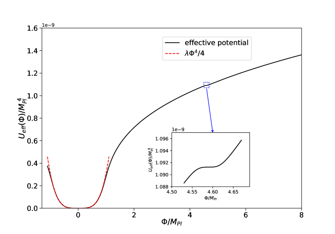
to change the non-canonical field to be the canonical field and get the effective potential for the model (3.3). In general, it is hard to get the analytical relation between the non-canonical field and the canonical field and to obtain the expression for the effective potential . However, we can use the numerical method to obtain the effective potential. For the only undetermined parameter in the peak function (3.5), we take
| (3.28) |
as an example to numerically obtain the effective potential which is shown in Figure 1. There is an inflection point in the effective potential and the existence of the inflection point in the effective potential is the reason why our model can enhance the power spectrum.
3.1 The results of the PBHs
In this section, we present the numerical results about the PBHs with the parameter taking the value in the equation (3.28).
The numerical solutions for the scalar tilt and the tensor-to-scalar ratio are
| (3.29) |
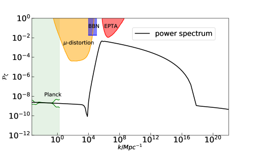
which are compatible with the Planck 2018 constraints [54] and the theoretic result (3.23), and the -folds before the end of inflation at the horizon exit for the pivotal scale are . The numerical solution for the primordial power spectrum is displayed in Figure 2, which is consistent with the constraints from the PTA observations [108], the effect on the ratio between neutron and proton during the big bang nucleosynthesis (BBN) [109] and -distortion of CMB [110]. The power spectrum at the peak and the peak scale are
| (3.30) |
By using the numerical results of the power spectrum of the primordial curvature perturbations, we obtain the PBHs mass function shown in Fig. 3.
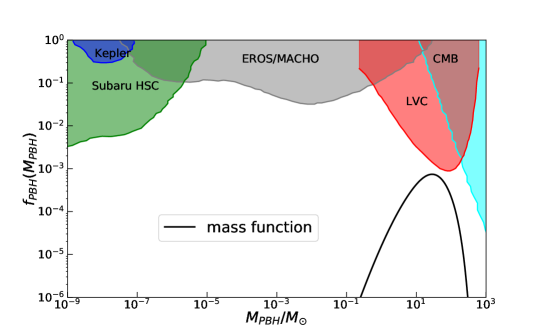
The PBHs mass and the mass function at the peak are
| (3.31) |
and the fraction of the PBHs in dark matter is
| (3.32) |
Therefore, for the case (3.28), we successfully produce the PBHs which can account for the LIGO-Virgo events, and the mass function is consistent with all the observational constraints.
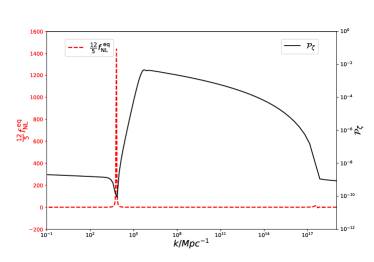
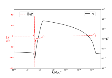
There may be some concern that the large enhancement on the power spectrum causes large non-Gaussianities which affect the formation of PBH DM. The non-Gaussianity parameter is
| (3.33) |
where and the definition of the bispectrum is
| (3.34) |
with being the quantum operator of the curvature perturbation . The influence of the non-Gaussianities on the abundance of PBHs can be characterized by the parameter
| (3.35) |
If , the effect of non-Gaussianities of the curvature perturbation on PBH abundance can be negligible. The numerical results for the non-Gaussianity parameter are shown in Figure 4. At the peak of the power spectrum, the non-Gaussianity parameter is small, so the effect of non-Gaussianities in our model is negligible.
3.2 The NANOGrav constraints and SIGWs
In this section, we apply the NANOGrav experimental results to obtain the constraints on the only undetermined parameter in the peak function (3.5). The results from the NANOGrav 12.5yrs data [1] are expressed in terms of the characteristic strain in the narrow frequency range with the power-law form
| (3.36) |
which can be related to the energy density of the GWs by
| (3.37) |
By combining equations (3.36) and (3.37), the predicted energy density of SIGWs in our model can be expanded as
| (3.38) |
with nHz [4] and
| (3.39) |
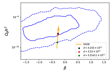
Using equation (3.39), we can transfer the experimental results of and to the constraints on the amplitude of SIGWs and the power index , which are shown in the left panel of Figure 5. The solid and dashed blue contours show the and constraints on the amplitude (nHz) [4] and power index indicated by the NANOGrav results [1], respectively. The orange line is the results of the SIGWs amplitude and power index from our model where the parameter increases along the arrow direction. The lower limit of satisfying the NANOGrav results is and marked by the green dot; the case (3.28) is marked by the red dot; the upper limit, from the constraints on the PBHs mass function, is and marked by the black dot. Therefore, the NANOGrav signal and the constraints on the PBHs require
| (3.40) |
The black dashed line in the right panel of Figure 5 denotes the PBHs mass function at the peak and satisfies , the black solid line denotes the fraction of the PBHs in dark matter and satisfies . For the allowed parameter region (3.40), the masses of the PBHs at the peak are around , the scalar tilt and tensor-to-scalar ratio are the same with equation (3.29), and the -folding numbers satisfy .
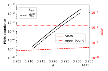
During BBN epoch, the SIGWs contribute to the total energy of extra relativistic species, and the energy density of the SIGWs should satisfy the following constraints [122]
| (3.41) |
where [123] is the upper bound on the effective number of relativistic degrees of freedom. The lower limit of the integral Hz [122] is the frequency of the mode entering the horizon at the BBN epoch, the upper limit of the integral Hz [124] is determined by the Hubble parameter at the end of inflation. The contributions to the total energy of extra relativistic species from the SIGWs of our model are shown in the right panel of the Figure 5 and denoted by the red dashed line which is consistent with the BBN constraints (3.41) denoted by the red dotted line.
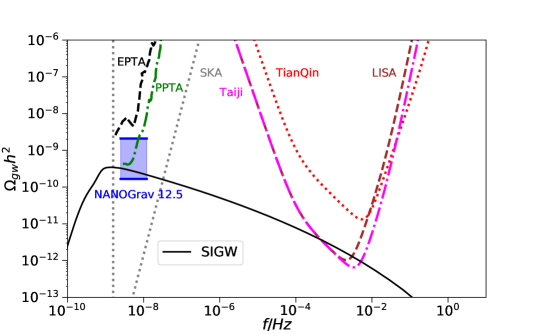
For the case (3.28), we display the energy density of the SIGWs as a function of the frequency in Figure 6. The frequencies of the SIGWs cover from nanohertz to millihertz. Around the nanohertz, the energy density of the SIGWs is consistent with the region of the NANOGrav signal; around the millihertz, the SIGWs can be detected by space-based GW detectors such as Taiji and LISA. This means that the NANOGrav signal may originate from the Higgs field and may also be detected by space-based GW detectors in the future.
4 Conclusion
The NANOGrav signal can be explained by the gravitational waves induced from large scalar perturbations at small scales during the radiation dominated epoch. By introducing a noncanonical kinetic term with a high peak in inflation models, the amplitude of the power spectrum of the primordial curvature perturbations can be enhanced to generate SIGWs and produce PBHs at small scales while keeping small to satisfy the Planck 2018 observational data at large scales. With this mechanism, the Higgs field successfully produces PBHs accounting for the LIGO-Virgo events and generates the SIGWs explaining the NANOGrav signal.
The PBHs observational constraints and the NANOGrav 12.5yrs experimental results require the parameter in the peak function to satisfy . Within this parameter range, the masses of the PBHs at the peak are around , the total fraction of the PBHs in dark matter satisfies . The scalar tilt and tensor-to-scalar ratio among these models are almost the same, which is and , and consistent with Planck 2018 observational data, the -folds for the pivot scale satisfy . The energy densities of the corresponding SIGWs are consistent with the region of the NANOGrav signal, and these SIGWs can be also detected by the future space-based GW detectors such as Taiji and LISA.
In conclusion, the NANOGrav signal and the BHs in LIGO-Virgo events can both originate from the Higgs field, and the NANOGrav signal may also be detected by the space-based GW detectors in the future.
Acknowledgments
This work is supported by the National Natural Science Foundation of China under Grants Nos. 11633001, 11920101003 and 12021003, the Strategic Priority Research Program of the Chinese Academy of Sciences, Grant No. XDB23000000 and the Interdiscipline Research Funds of Beijing Normal University. Z. Y. thanks Fengge Zhang for the useful discussion.
References
- [1] NANOGrav collaboration, The nanograv 12.5 yr data set: Search for an isotropic stochastic gravitational-wave background, Astrophys. J. Lett. 905 (2020) L34 [2009.04496].
- [2] V. De Luca, G. Franciolini and A. Riotto, Nanograv data hints at primordial black holes as dark matter, Phys. Rev. Lett. 126 (2021) 041303 [2009.08268].
- [3] K. Inomata, M. Kawasaki, K. Mukaida and T.T. Yanagida, Nanograv results and ligo-virgo primordial black holes in axionlike curvaton models, Phys. Rev. Lett. 126 (2021) 131301 [2011.01270].
- [4] V. Vaskonen and H. Veermäe, Did nanograv see a signal from primordial black hole formation?, Phys. Rev. Lett. 126 (2021) 051303 [2009.07832].
- [5] K. Kohri and T. Terada, Solar-mass primordial black holes explain nanograv hint of gravitational waves, Phys. Lett. B 813 (2021) 136040 [2009.11853].
- [6] G. Domènech and S. Pi, Nanograv hints on planet-mass primordial black holes, 2010.03976.
- [7] S. Vagnozzi, Implications of the nanograv results for inflation, Mon. Not. Roy. Astron. Soc. 502 (2021) L11 [2009.13432].
- [8] M. Kawasaki and H. Nakatsuka, Gravitational waves from type II axion-like curvaton model and its implication for NANOGrav result, JCAP 05 (2021) 023 [2101.11244].
- [9] S. Blasi, V. Brdar and K. Schmitz, Has nanograv found first evidence for cosmic strings?, Phys. Rev. Lett. 126 (2021) 041305 [2009.06607].
- [10] J. Ellis and M. Lewicki, Cosmic string interpretation of nanograv pulsar timing data, Phys. Rev. Lett. 126 (2021) 041304 [2009.06555].
- [11] S.-L. Li, L. Shao, P. Wu and H. Yu, NANOGrav signal from first-order confinement-deconfinement phase transition in different QCD-matter scenarios, Phys. Rev. D 104 (2021) 043510 [2101.08012].
- [12] V. Atal, A. Sanglas and N. Triantafyllou, NANOGrav signal as mergers of Stupendously Large Primordial Black Holes, JCAP 06 (2021) 022 [2012.14721].
- [13] Z.-C. Chen, C. Yuan and Q.-G. Huang, Non-tensorial gravitational wave background in NANOGrav 12.5-year data set, Sci. China Phys. Mech. Astron. 64 (2021) 120412 [2101.06869].
- [14] N. Ramberg and L. Visinelli, Qcd axion and gravitational waves in light of nanograv results, Phys. Rev. D 103 (2021) 063031 [2012.06882].
- [15] H. Middleton, A. Sesana, S. Chen, A. Vecchio, W. Del Pozzo and P.A. Rosado, Massive black hole binary systems and the nanograv 12.5 year results, Mon. Not. Roy. Astron. Soc. 502 (2021) L99 [2011.01246].
- [16] H.-H. Li, G. Ye and Y.-S. Piao, Is the nanograv signal a hint of ds decay during inflation?, Phys. Lett. B 816 (2021) 136211 [2009.14663].
- [17] Y. Cai and Y.-S. Piao, Intermittent null energy condition violations during inflation and primordial gravitational waves, Phys. Rev. D 103 (2021) 083521 [2012.11304].
- [18] S. Bhattacharya, S. Mohanty and P. Parashari, Implications of the nanograv result on primordial gravitational waves in nonstandard cosmologies, Phys. Rev. D 103 (2021) 063532 [2010.05071].
- [19] A.K. Pandey, Gravitational waves in neutrino plasma and NANOGrav signal, Eur. Phys. J. C 81 (2021) 399 [2011.05821].
- [20] L. Bian, R.-G. Cai, J. Liu, X.-Y. Yang and R. Zhou, Evidence for different gravitational-wave sources in the nanograv dataset, Phys. Rev. D 103 (2021) L081301.
- [21] R. Sharma, Constraining models of inflationary magnetogenesis with nanograv, 2102.09358.
- [22] S. Kuroyanagi, T. Takahashi and S. Yokoyama, Blue-tilted inflationary tensor spectrum and reheating in the light of nanograv results, JCAP 01 (2021) 071 [2011.03323].
- [23] W. Ratzinger and P. Schwaller, Whispers from the dark side: Confronting light new physics with nanograv data, SciPost Phys. 10 (2021) 047 [2009.11875].
- [24] R. Samanta and S. Datta, Gravitational wave complementarity and impact of NANOGrav data on gravitational leptogenesis: cosmic strings, 2009.13452.
- [25] S. Bird, I. Cholis, J.B. Muñoz, Y. Ali-Haïmoud, M. Kamionkowski, E.D. Kovetz et al., Did LIGO detect dark matter?, Phys. Rev. Lett. 116 (2016) 201301 [1603.00464].
- [26] M. Sasaki, T. Suyama, T. Tanaka and S. Yokoyama, Primordial Black Hole Scenario for the Gravitational-Wave Event GW150914, Phys. Rev. Lett. 117 (2016) 061101 [1603.08338].
- [27] LIGO Scientific, Virgo collaboration, Observation of Gravitational Waves from a Binary Black Hole Merger, Phys. Rev. Lett. 116 (2016) 061102 [1602.03837].
- [28] LIGO Scientific, Virgo collaboration, GW151226: Observation of Gravitational Waves from a 22-Solar-Mass Binary Black Hole Coalescence, Phys. Rev. Lett. 116 (2016) 241103 [1606.04855].
- [29] LIGO Scientific, VIRGO collaboration, GW170104: Observation of a 50-Solar-Mass Binary Black Hole Coalescence at Redshift 0.2, Phys. Rev. Lett. 118 (2017) 221101 [1706.01812].
- [30] LIGO Scientific, Virgo collaboration, GW170814: A Three-Detector Observation of Gravitational Waves from a Binary Black Hole Coalescence, Phys. Rev. Lett. 119 (2017) 141101 [1709.09660].
- [31] LIGO Scientific, Virgo collaboration, GW170817: Observation of Gravitational Waves from a Binary Neutron Star Inspiral, Phys. Rev. Lett. 119 (2017) 161101 [1710.05832].
- [32] LIGO Scientific, Virgo collaboration, GW170608: Observation of a 19-solar-mass Binary Black Hole Coalescence, Astrophys. J. 851 (2017) L35 [1711.05578].
- [33] LIGO Scientific, Virgo collaboration, GWTC-1: A Gravitational-Wave Transient Catalog of Compact Binary Mergers Observed by LIGO and Virgo during the First and Second Observing Runs, Phys. Rev. X 9 (2019) 031040 [1811.12907].
- [34] LIGO Scientific, Virgo collaboration, Gw190425: Observation of a compact binary coalescence with total mass , Astrophys. J. Lett. 892 (2020) L3 [2001.01761].
- [35] LIGO Scientific, Virgo collaboration, Gw190412: Observation of a binary-black-hole coalescence with asymmetric masses, Phys. Rev. D 102 (2020) 043015 [2004.08342].
- [36] LIGO Scientific, Virgo collaboration, Gw190814: Gravitational waves from the coalescence of a 23 solar mass black hole with a 2.6 solar mass compact object, Astrophys. J. Lett. 896 (2020) L44 [2006.12611].
- [37] LIGO Scientific, Virgo collaboration, Gw190521: A binary black hole merger with a total mass of , Phys. Rev. Lett. 125 (2020) 101102 [2009.01075].
- [38] LIGO Scientific, Virgo collaboration, GWTC-2: Compact Binary Coalescences Observed by LIGO and Virgo During the First Half of the Third Observing Run, Phys. Rev. X 11 (2021) 021053 [2010.14527].
- [39] P. Ivanov, P. Naselsky and I. Novikov, Inflation and primordial black holes as dark matter, Phys. Rev. D 50 (1994) 7173.
- [40] P.H. Frampton, M. Kawasaki, F. Takahashi and T.T. Yanagida, Primordial Black Holes as All Dark Matter, JCAP 04 (2010) 023 [1001.2308].
- [41] K. Belotsky, A. Dmitriev, E. Esipova, V. Gani, A. Grobov, M.Y. Khlopov et al., Signatures of primordial black hole dark matter, Mod. Phys. Lett. A 29 (2014) 1440005 [1410.0203].
- [42] M.Y. Khlopov, S.G. Rubin and A.S. Sakharov, Primordial structure of massive black hole clusters, Astropart. Phys. 23 (2005) 265 [astro-ph/0401532].
- [43] S. Clesse and J. García-Bellido, Massive Primordial Black Holes from Hybrid Inflation as Dark Matter and the seeds of Galaxies, Phys. Rev. D 92 (2015) 023524 [1501.07565].
- [44] B. Carr, F. Kuhnel and M. Sandstad, Primordial black holes as dark matter, Phys. Rev. D 94 (2016) 083504 [1607.06077].
- [45] K. Inomata, M. Kawasaki, K. Mukaida, Y. Tada and T.T. Yanagida, Inflationary Primordial Black Holes as All Dark Matter, Phys. Rev. D 96 (2017) 043504 [1701.02544].
- [46] J. García-Bellido, Massive Primordial Black Holes as Dark Matter and their detection with Gravitational Waves, J. Phys. Conf. Ser. 840 (2017) 012032 [1702.08275].
- [47] E.D. Kovetz, Probing Primordial-Black-Hole Dark Matter with Gravitational Waves, Phys. Rev. Lett. 119 (2017) 131301 [1705.09182].
- [48] S. Pi, Y.-l. Zhang, Q.-G. Huang and M. Sasaki, Scalaron from -gravity as a heavy field, JCAP 05 (2018) 042 [1712.09896].
- [49] R.-g. Cai, S. Pi and M. Sasaki, Gravitational Waves Induced by non-Gaussian Scalar Perturbations, Phys. Rev. Lett. 122 (2019) 201101 [1810.11000].
- [50] B. Carr and F. Kuhnel, Primordial black holes as dark matter: Recent developments, Ann. Rev. Nucl. Part. Sci. 70 (2020) 355 [2006.02838].
- [51] J. Scholtz and J. Unwin, What if Planet 9 is a Primordial Black Hole?, Phys. Rev. Lett. 125 (2020) 051103 [1909.11090].
- [52] B.J. Carr and S.W. Hawking, Black holes in the early Universe, Mon. Not. Roy. Astron. Soc. 168 (1974) 399.
- [53] S. Hawking, Gravitationally collapsed objects of very low mass, Mon. Not. Roy. Astron. Soc. 152 (1971) 75.
- [54] Planck collaboration, Planck 2018 results. X. Constraints on inflation, Astron. Astrophys. 641 (2020) A10 [1807.06211].
- [55] H. Di and Y. Gong, Primordial black holes and second order gravitational waves from ultra-slow-roll inflation, JCAP 1807 (2018) 007 [1707.09578].
- [56] Y. Lu, Y. Gong, Z. Yi and F. Zhang, Constraints on primordial curvature perturbations from primordial black hole dark matter and secondary gravitational waves, JCAP 12 (2019) 031 [1907.11896].
- [57] G. Sato-Polito, E.D. Kovetz and M. Kamionkowski, Constraints on the primordial curvature power spectrum from primordial black holes, Phys. Rev. D 100 (2019) 063521 [1904.10971].
- [58] J. Martin, H. Motohashi and T. Suyama, Ultra Slow-Roll Inflation and the non-Gaussianity Consistency Relation, Phys. Rev. D 87 (2013) 023514 [1211.0083].
- [59] H. Motohashi, A.A. Starobinsky and J. Yokoyama, Inflation with a constant rate of roll, JCAP 1509 (2015) 018 [1411.5021].
- [60] Z. Yi and Y. Gong, On the constant-roll inflation, JCAP 1803 (2018) 052 [1712.07478].
- [61] J. Garcia-Bellido and E. Ruiz Morales, Primordial black holes from single field models of inflation, Phys. Dark Univ. 18 (2017) 47 [1702.03901].
- [62] C. Germani and T. Prokopec, On primordial black holes from an inflection point, Phys. Dark Univ. 18 (2017) 6 [1706.04226].
- [63] H. Motohashi and W. Hu, Primordial black holes and slow-roll violation, Phys. Rev. D 96 (2017) 063503 [1706.06784].
- [64] J.M. Ezquiaga, J. Garcia-Bellido and E. Ruiz Morales, Primordial Black Hole production in Critical Higgs Inflation, Phys. Lett. B 776 (2018) 345 [1705.04861].
- [65] G. Ballesteros, J. Beltran Jimenez and M. Pieroni, Black hole formation from a general quadratic action for inflationary primordial fluctuations, JCAP 1906 (2019) 016 [1811.03065].
- [66] I. Dalianis, A. Kehagias and G. Tringas, Primordial black holes from -attractors, JCAP 01 (2019) 037 [1805.09483].
- [67] A.Y. Kamenshchik, A. Tronconi, T. Vardanyan and G. Venturi, Non-Canonical Inflation and Primordial Black Holes Production, Phys. Lett. B 791 (2019) 201 [1812.02547].
- [68] C. Fu, P. Wu and H. Yu, Primordial Black Holes from Inflation with Nonminimal Derivative Coupling, Phys. Rev. D 100 (2019) 063532 [1907.05042].
- [69] C. Fu, P. Wu and H. Yu, Scalar induced gravitational waves in inflation with gravitationally enhanced friction, Phys. Rev. D 101 (2020) 023529 [1912.05927].
- [70] I. Dalianis, S. Karydas and E. Papantonopoulos, Generalized non-minimal derivative coupling: Application to inflation and primordial black hole production, JCAP 06 (2020) 040 [1910.00622].
- [71] J. Lin, Q. Gao, Y. Gong, Y. Lu, C. Zhang and F. Zhang, Primordial black holes and secondary gravitational waves from and inflation, Phys. Rev. D 101 (2020) 103515 [2001.05909].
- [72] M. Braglia, D.K. Hazra, F. Finelli, G.F. Smoot, L. Sriramkumar and A.A. Starobinsky, Generating pbhs and small-scale gws in two-field models of inflation, JCAP 08 (2020) 001 [2005.02895].
- [73] A. Gundhi and C.F. Steinwachs, Scalaron–Higgs inflation reloaded: Higgs-dependent scalaron mass and primordial black hole dark matter, Eur. Phys. J. C 81 (2021) 460 [2011.09485].
- [74] D.Y. Cheong, S.M. Lee and S.C. Park, Primordial black holes in Higgs- inflation as the whole of dark matter, JCAP 01 (2021) 032 [1912.12032].
- [75] Q. Gao, Primordial black holes and secondary gravitational waves from chaotic inflation, Sci. China Phys. Mech. Astron. 64 (2021) 280411 [2102.07369].
- [76] J. Lin, S. Gao, Y. Gong, Y. Lu, Z. Wang and F. Zhang, Primordial black holes and scalar induced secondary gravitational waves from higgs inflation with non-canonical kinetic term, 2111.01362.
- [77] F. Zhang, Primordial black holes and scalar induced gravitational waves from the E model with a Gauss-Bonnet term, Phys. Rev. D 105 (2022) 063539 [2112.10516].
- [78] Z. Yi, Q. Gao, Y. Gong and Z.-H. Zhu, Primordial black holes and scalar-induced secondary gravitational waves from inflationary models with a noncanonical kinetic term, Phys. Rev. D 103 (2021) 063534 [2011.10606].
- [79] Z. Yi, Y. Gong, B. Wang and Z.-H. Zhu, Primordial black holes and secondary gravitational waves from the higgs field, Phys. Rev. D 103 (2021) 063535 [2007.09957].
- [80] Q. Gao, Y. Gong and Z. Yi, Primordial black holes and secondary gravitational waves from natural inflation, Nucl. Phys. B 969 (2021) 115480 [2012.03856].
- [81] ATLAS collaboration, Observation of a new particle in the search for the standard model higgs boson with the atlas detector at the lhc, Phys. Lett. B 716 (2012) 1 [1207.7214].
- [82] CMS collaboration, Observation of a new boson at a mass of 125 gev with the cms experiment at the lhc, Phys. Lett. B 716 (2012) 30 [1207.7235].
- [83] Particle Data Group collaboration, Review of particle physics, Phys. Rev. D 98 (2018) 030001.
- [84] J.M. Bardeen, J.R. Bond, N. Kaiser and A.S. Szalay, The Statistics of Peaks of Gaussian Random Fields, Astrophys. J. 304 (1986) 15.
- [85] A.M. Green, A.R. Liddle, K.A. Malik and M. Sasaki, A New calculation of the mass fraction of primordial black holes, Phys. Rev. D 70 (2004) 041502 [astro-ph/0403181].
- [86] S. Young, C.T. Byrnes and M. Sasaki, Calculating the mass fraction of primordial black holes, JCAP 07 (2014) 045 [1405.7023].
- [87] C. Germani and I. Musco, The abundance of primordial black holes depends on the shape of the inflationary power spectrum, Phys. Rev. Lett. 122 (2019) 141302 [1805.04087].
- [88] S. Young and M. Musso, Application of peaks theory to the abundance of primordial black holes, JCAP 11 (2020) 022 [2001.06469].
- [89] A.D. Gow, C.T. Byrnes, P.S. Cole and S. Young, The power spectrum on small scales: Robust constraints and comparing pbh methodologies, JCAP 02 (2021) 002 [2008.03289].
- [90] I. Musco, Threshold for primordial black holes: Dependence on the shape of the cosmological perturbations, Phys. Rev. D 100 (2019) 123524 [1809.02127].
- [91] S. Young, The primordial black hole formation criterion re-examined: Parametrisation, timing and the choice of window function, Int. J. Mod. Phys. D 29 (2019) 2030002 [1905.01230].
- [92] M.W. Choptuik, Universality and scaling in gravitational collapse of a massless scalar field, Phys. Rev. Lett. 70 (1993) 9.
- [93] C.R. Evans and J.S. Coleman, Observation of critical phenomena and selfsimilarity in the gravitational collapse of radiation fluid, Phys. Rev. Lett. 72 (1994) 1782 [gr-qc/9402041].
- [94] J.C. Niemeyer and K. Jedamzik, Near-critical gravitational collapse and the initial mass function of primordial black holes, Phys. Rev. Lett. 80 (1998) 5481 [astro-ph/9709072].
- [95] C.T. Byrnes, M. Hindmarsh, S. Young and M.R.S. Hawkins, Primordial black holes with an accurate qcd equation of state, JCAP 08 (2018) 041 [1801.06138].
- [96] K. Danzmann, Lisa: An esa cornerstone mission for a gravitational wave observatory, Class. Quant. Grav. 14 (1997) 1399.
- [97] H. Audley et al., Laser Interferometer Space Antenna, 1702.00786.
- [98] W.-R. Hu and Y.-L. Wu, The taiji program in space for gravitational wave physics and the nature of gravity, Natl. Sci. Rev. 4 (2017) 685.
- [99] TianQin collaboration, TianQin: a space-borne gravitational wave detector, Class. Quant. Grav. 33 (2016) 035010 [1512.02076].
- [100] K.N. Ananda, C. Clarkson and D. Wands, The Cosmological gravitational wave background from primordial density perturbations, Phys. Rev. D 75 (2007) 123518 [gr-qc/0612013].
- [101] D. Baumann, P.J. Steinhardt, K. Takahashi and K. Ichiki, Gravitational Wave Spectrum Induced by Primordial Scalar Perturbations, Phys. Rev. D 76 (2007) 084019 [hep-th/0703290].
- [102] K. Kohri and T. Terada, Semianalytic calculation of gravitational wave spectrum nonlinearly induced from primordial curvature perturbations, Phys. Rev. D 97 (2018) 123532 [1804.08577].
- [103] J.R. Espinosa, D. Racco and A. Riotto, A Cosmological Signature of the SM Higgs Instability: Gravitational Waves, JCAP 1809 (2018) 012 [1804.07732].
- [104] T. Kobayashi, M. Yamaguchi and J. Yokoyama, G-inflation: Inflation driven by the Galileon field, Phys. Rev. Lett. 105 (2010) 231302 [1008.0603].
- [105] J. Garriga and V.F. Mukhanov, Perturbations in k-inflation, Phys. Lett. B 458 (1999) 219 [hep-th/9904176].
- [106] C. Armendariz-Picon, T. Damour and V.F. Mukhanov, k - inflation, Phys. Lett. B 458 (1999) 209 [hep-th/9904075].
- [107] J. Lin, Q. Gao and Y. Gong, The reconstruction of inflationary potentials, Mon. Not. Roy. Astron. Soc. 459 (2016) 4029 [1508.07145].
- [108] K. Inomata and T. Nakama, Gravitational waves induced by scalar perturbations as probes of the small-scale primordial spectrum, Phys. Rev. D 99 (2019) 043511 [1812.00674].
- [109] K. Inomata, M. Kawasaki and Y. Tada, Revisiting constraints on small scale perturbations from big-bang nucleosynthesis, Phys. Rev. D 94 (2016) 043527 [1605.04646].
- [110] D.J. Fixsen, E.S. Cheng, J.M. Gales, J.C. Mather, R.A. Shafer and E.L. Wright, The Cosmic Microwave Background spectrum from the full COBE FIRAS data set, Astrophys. J. 473 (1996) 576 [astro-ph/9605054].
- [111] Y. Ali-Haïmoud and M. Kamionkowski, Cosmic microwave background limits on accreting primordial black holes, Phys. Rev. D 95 (2017) 043534 [1612.05644].
- [112] V. Poulin, P.D. Serpico, F. Calore, S. Clesse and K. Kohri, Cmb bounds on disk-accreting massive primordial black holes, Phys. Rev. D 96 (2017) 083524 [1707.04206].
- [113] Y. Ali-Haïmoud, E.D. Kovetz and M. Kamionkowski, Merger rate of primordial black-hole binaries, Phys. Rev. D 96 (2017) 123523 [1709.06576].
- [114] M. Raidal, C. Spethmann, V. Vaskonen and H. Veermäe, Formation and evolution of primordial black hole binaries in the early universe, JCAP 02 (2019) 018 [1812.01930].
- [115] V. Vaskonen and H. Veermäe, Lower bound on the primordial black hole merger rate, Phys. Rev. D 101 (2020) 043015 [1908.09752].
- [116] V. De Luca, G. Franciolini, P. Pani and A. Riotto, Primordial black holes confront ligo/virgo data: Current situation, JCAP 06 (2020) 044 [2005.05641].
- [117] K.W.K. Wong, G. Franciolini, V. De Luca, V. Baibhav, E. Berti, P. Pani et al., Constraining the primordial black hole scenario with bayesian inference and machine learning: the gwtc-2 gravitational wave catalog, Phys. Rev. D 103 (2021) 023026 [2011.01865].
- [118] G. Hütsi, M. Raidal, V. Vaskonen and H. Veermäe, Two populations of ligo-virgo black holes, JCAP 03 (2021) 068 [2012.02786].
- [119] EROS-2 collaboration, Limits on the Macho Content of the Galactic Halo from the EROS-2 Survey of the Magellanic Clouds, Astron. Astrophys. 469 (2007) 387 [astro-ph/0607207].
- [120] H. Niikura et al., Microlensing constraints on primordial black holes with Subaru/HSC Andromeda observations, Nat. Astron. 3 (2019) 524 [1701.02151].
- [121] K. Griest, A.M. Cieplak and M.J. Lehner, New Limits on Primordial Black Hole Dark Matter from an Analysis of Kepler Source Microlensing Data, Phys. Rev. Lett. 111 (2013) 181302.
- [122] S. Kuroyanagi, T. Takahashi and S. Yokoyama, Blue-tilted inflationary tensor spectrum and reheating in the light of NANOGrav results, .
- [123] R.H. Cyburt, B.D. Fields, K.A. Olive and T.-H. Yeh, Big bang nucleosynthesis: Present status, .
- [124] S. Kuroyanagi, T. Takahashi and S. Yokoyama, Blue-tilted tensor spectrum and thermal history of the Universe, .
- [125] R. Ferdman et al., The european pulsar timing array: current efforts and a leap toward the future, Class. Quant. Grav. 27 (2010) 084014 [1003.3405].
- [126] G. Hobbs et al., The international pulsar timing array project: using pulsars as a gravitational wave detector, Class. Quant. Grav. 27 (2010) 084013 [0911.5206].
- [127] M.A. McLaughlin, The north american nanohertz observatory for gravitational waves, Class. Quant. Grav. 30 (2013) 224008 [1310.0758].
- [128] G. Hobbs, The parkes pulsar timing array, Class. Quant. Grav. 30 (2013) 224007 [1307.2629].
- [129] L. Lentati et al., European pulsar timing array limits on an isotropic stochastic gravitational-wave background, Mon. Not. Roy. Astron. Soc. 453 (2015) 2576 [1504.03692].
- [130] R.M. Shannon et al., Gravitational waves from binary supermassive black holes missing in pulsar observations, Science 349 (2015) 1522 [1509.07320].
- [131] C. Moore, R. Cole and C. Berry, Gravitational-wave sensitivity curves, Class. Quant. Grav. 32 (2015) 015014 [1408.0740].