MaNGA galaxy properties – I. An extensive optical, mid-infrared photometric, and environmental catalogue

Abstract

We present an extensive catalogueue of non-parametric structural properties derived from optical and mid-infrared imaging for 4585 galaxies from the MaNGA survey. DESI and Wide-field Infrared Survey (WISE) imaging are used to extract surface brightness profiles in the $g,r,z,{\it W1},W2$ photometric bands. Our optical photometry takes advantage of the automated algorithm AUTOPROF and probes surface brightnesses that typically reach below 29 ${{{{\rm mag}~{}{\rm arcsec}}^{-2}}}$ in the $r$ band, while our WISE photometry achieves 28 ${{{{\rm mag}~{}{\rm arcsec}}^{-2}}}$ in the ${\it W1}$ band. Neighbour density measures and central/satellite classifications are also provided for a large subsample of the MaNGA galaxies. Highlights of our analysis of galaxy light profiles include (i) an extensive comparison of galaxian structural properties that illustrates the robustness of non-parametric extraction of light profiles over parametric methods; (ii) the ubiquity of bimodal structural properties, suggesting the existence of galaxy families in multiple dimensions; and (iii) an appreciation that structural properties measured relative to total light, regardless of the fractional level, are uncertain. We study galaxy scaling relations based on photometric parameters, and present detailed comparisons with literature and theory. Salient features of this analysis include the near-constancy of the slope and scatter of the size–luminosity and size–stellar mass relations for late-type galaxies with wavelength, and the saturation of the central surface density, measured within 1 kpc, for elliptical galaxies with $M_{*}>10.7\,M_{\odot}$ (corresponding to $\Sigma_{1}\simeq 10^{10}\,M_{\odot}\,{\rm kpc}^{-2}$). The multiband photometry, environmental parameters, and structural scaling relations presented are useful constraints for stellar population and galaxy formation models.

1 Introduction

A comprehensive picture of galaxy formation and evolution, as well as reliable data-model comparisons, requires access to large homogeneous photometric and spectroscopic samples of galaxies covering a broad range of morphologies, stellar and dynamical masses, star formation histories, environmental conditions, and more. Previously, such measurements have been extracted from large imaging and spectroscopic wide-field surveys such as 2MASS (Jarrett et al., 2000), SDSS (York et al., 2000), GAMA (Driver et al., 2009), and others. More recently, large-scale acquisition of spatially resolved structural properties of galaxies has been achieved with integral-field spectroscopy. The latter is especially valuable in this context since it allows the synchronous collection of global and spatially resolved chemical and dynamical properties such as stellar mass surface density, age, metallicities, star formation rates, circular velocity, velocity dispersion and more, across a broad wavelength range. Pioneering integral-field spectroscopy surveys of galaxies such as SAURON (Bacon et al., 2001), ATLAS^3D (Cappellari et al., 2011), CALIFA (Walcher et al., 2014), and SAMI (Allen et al., 2015), provide such properties, although for relatively small samples.

With its spatially resolved optical spectroscopic data for ${\sim}10000$ nearby galaxies ($z{\sim}0.15$), the SDSS-IV survey “Mapping Nearby Galaxy at Apache point observatory" (MaNGA; Bundy et al., 2015; Wake et al., 2017) has heralded a new era of large-scale galaxy studies with integral field units (IFUs). MaNGA uses a 127-fiber IFU to provide high-quality spatially resolved kinematic and chemical information for galaxies by collecting spectra at each pixel out to a maximum of 1.5/2.5 effective radii ($R_{\rm eff}$) for 85/15 percent of the MaNGA sample (Cano-Díaz et al., 2016; Sánchez et al., 2016, 2018; Graham et al., 2018; Méndez-Abreu et al., 2018). The MaNGA galaxies were selected from the NSA catalogue with no inclination or size selection cuts. For more details about the MaNGA sample, see Bundy et al. (2015) and Wake et al. (2017).

Large-scale IFU surveys, such as MaNGA and CALIFA (Walcher et al., 2014), open an avenue for the exploration of spatially resolved counterparts to global structural drivers and scaling relations in galaxies. For instance, the MaNGA survey has already yielded new insights about evolutionary mechanisms such as star formation quenching; finding it to be regulated on global galaxy scales while star formation density is controlled locally (Bluck et al., 2020). Using the Pipe3D (Sánchez et al., 2018) output for MaNGA, Sánchez-Menguiano et al. (2020) have also explored the relation between the average stellar age and gas-phase metallicity for star-forming systems. While this relation had been observed globally (Lian et al., 2015), the spatially resolved nature of the MaNGA data also revealed a local correlation.

In addition to the published spatially resolved spectroscopic MaNGA data, a comprehensive understanding of MaNGA galaxies requires a full suite of structural and environmental galaxy properties. A catalogue of model-dependent MaNGA galaxy structural parameters (effective sizes, total magnitudes, Sérsic indices, ellipticities, position angles) already exists (Fischer et al., 2019, hereafter F19). The MaNGA PYMORPH Photometric Value Added Catalogue (MPP-VAC) provides structural parameters for MaNGA galaxies extracted through Sérsic and Sérsic+Exponential fits to 2D surface brightness profiles. However, model-dependent assumptions about the light distribution of galaxies severely bias and limit any investigations of galaxy structure and evolution, as shown below. Providing galaxy structural parameters in non-parametric fashion is the main goal of this study.

In this paper, we present an extensive compilation of model-independent galaxian structural parameters based on optical and mid-infrared (MIR) imaging of all MaNGA galaxies extracted respectively from the Dark Energy Sky Instrument Legacy Imaging Survey (DESI Collaboration et al., 2016; Dey et al., 2019) and Wide-field Infrared Survey Explorer (WISE) surveys. The combination of optical and MIR bands is especially sensitive to the evolved stellar population, sites of star formation, and distribution of dust within galaxies. Broader multiband coverage for MaNGA galaxies is also being developed elsewhere; major imaging campaigns of MaNGA galaxies at radio (Masters et al., 2019) and ultraviolet wavelengths (Molina et al., 2020) are either in place or in progress. These will expand our understanding of MaNGA galaxies with clearer views of processes such as star formation on small spatial/time scales and the distribution of neutral hydrogen within galaxies, the fuel for star formation.

The surface brightness (surface brightness) profiles extracted from the DESI and WISE imaging surveys for the MaNGA galaxies allow us to extract numerous non-parametric structural properties representing various measures of galaxy size, surface brightness, luminosity, stellar mass, and stellar mass surface density. Along with the structural parameters for MaNGA galaxies, environmental demographics are also provided below. Our compilation supplements fifth nearest-neighbour density measurements for MaNGA galaxies (see Argudo-Fernández et al., 2015; Etherington & Thomas, 2015, for details), with important information about the gravitational dominance of a galaxy (i.e. central and satellite designation) within its own halo. These considerations motivate the assembly of a catalogue of environmental properties for a large subsample of MaNGA galaxies, in addition to the photometric catalogues. The environmental catalogue that we present below includes measures of neighbour densities and classification of these galaxies as a central or satellite.

A natural outcome of such an extensive data compilation is the construction and study of galaxy scaling relations. The slope, zero-point, and scatter of such empirical scaling relations present evidence of the underlying physics that dictates structure formation and evolution of galaxies (Mo et al., 1998; Courteau et al., 2007; Dutton et al., 2007; Brook et al., 2012; Hall et al., 2012; Lange et al., 2015). The MaNGA non-parametric data sets produced in this study allow for an analysis of various galaxy scaling relations in different photometric bands. Among others, the size–stellar mass ($R-M_{*}$) relation and the stellar surface density ($\Sigma_{1}$ measured within 1 kpc) - stellar mass relations ($\Sigma_{1}-M_{*}$) are presented. As discussed below, these relations enable constraints of the gas accretion and merger history as well as quenching and feedback models in galaxies (Chiosi & Carraro, 2002; Shen et al., 2003; Franx et al., 2008; Saglia et al., 2010; Fang et al., 2013; Woo & Ellison, 2019).

This paper is organized as follows: in Section 2, we describe the procedures used to extract surface brightness profiles in optical and MIR bands. The extraction and correction of non-parametric galaxy structural properties are also discussed and presented in tabular format. The environmental catalogue is presented in Section 2.2.5. With our catalogue in place, we provide in Section 3 a broad overview of the DESI and WISE parameters for our MaNGA Public sample. Unimodal and bimodal structural distributions are also highlighted. In Section 4, we compare our model-independent structural parameters for MaNGA galaxies, such as size, apparent magnitude, and stellar mass, with literature values. Our MIR photometry and derived structural properties are compared to optical structural properties in Section 5. With our optical and MIR photometry validated, we combine these data sets in Section 6 to infer structural galaxy scaling relations of MaNGA galaxies with a focus on the size–stellar mass, $R-M_{*}$, relation in Section 6.1, and the central surface density–stellar mass, $\Sigma_{1}-M_{*}$, relation in Section 6.3. We conclude in Section 7.

2 Light Profile Extraction

Our galaxy sample consists of 4585 galaxies from the public release of the MaNGA survey. The full MaNGA galaxy survey will yield $\sim$10 000 objects with a uniform distribution of stellar mass $M_{*}>10^{9}{\rm M_{\odot}}$, with no inclination or size selections.

For our optical photometry, we have cross-correlated the public MaNGA data release with the DESI (DESI Collaboration et al., 2016) and extracted $\rm 10\times 10\,{arcmin^{2}}$ images in the g, r, and z bands for 4585 matching galaxies. The large galaxy images ensure that the background sky level can be robustly characterized and subtracted. We use our fully automated ‘AUTOPROF ’ code (Section 2.1) to extract azimuthally averaged surface brightness profiles from DESI g-,r- and z- band images, with the solution fit to the r band for its minimal dust extinction and high signal-to-noise ratio (S/N; and for consistency with the parallel Photometry and Rotation Curve Observations from Extragalactic Surveys, or “PROBES”, investigation by Stone & Courteau 2019 and Stone et al. 2021). The $r$-band isophotal solution is applied to the $g$ and $z$ images for uniformity of the position angles, ellipticities, fluxes and color gradients. Unless otherwise stated, all band-dependent structural parameters refer to the $z$ band photometry. The automation of AUTOPROF is well suited to large surveys like DESI, where interactive surface brightness extraction methods, such as those based on the XVISTA data reduction package, become prohibitive (see Courteau, 1996; McDonald et al., 2011; Hall et al., 2012; Gilhuly & Courteau, 2018, for more details).

Our MIR surface brightness profiles are derived from the WISE Large Galaxy Atlas and the Extended Source catalogue (WXSC; Jarrett et al. 2019), which features custom image mosaic construction to produce native angular resolution products that include both WISE and NEOWISE imaging to improve the sensitivity; complete details of image construction are provided in Jarrett et al. (2012). Here we use the W1 (3.4$\rm\mu$m) and W2 (4.6$\rm\mu$m) mosaics with 5.9$\scriptscriptstyle\prime$ $\scriptscriptstyle\prime$ and 6.5$\scriptscriptstyle\prime$ $\scriptscriptstyle\prime$ spatial resolution, respectively. These bands are sensitive to the evolved stellar populations (Jarrett et al., 2013), and hence the stellar mass content and distribution for the target galaxies. We have extracted from the WISE surface brightness profiles the same structural properties as those measured from the DESI optical photometry, except for the stellar surface density within 1 kpc which is not resolved for many WISE profiles. The robustness of our WISE derived structural properties is demonstrated in Section 5. Among others, the W1 and W2 band passes are especially sensitive to older, more mass dominant stellar populations resulting in robust stellar mass measurements. The comparison of stellar masses from our DESI and WISE photometry is presented in Section 5. In what follows, all surface brightnesses used and reported are in the AB magnitude system.

In Appendix A, we provide Table 8 and 9 to present the output format of the public multiband surface brightness profiles.

2.1 AUTOPROF

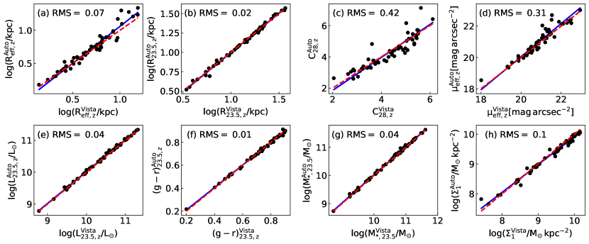
Figure 1: Comparison of photometrically derived non-parametric quantities from XVISTA interactive routines and AUTOPROF with: (panel a) effective radius [$R_{\rm eff}$], (panel b) isophotal radius [$R_{\rm 23.5}$], (panel c) concentration index [$C_{\rm 28}$], (panel d) effective surface brightness [$\mu_{eff}$], (panel e) luminosity within $R_{\rm 23.5}$ [$L_{\rm 23.5}$], (panel f) colour within $R_{\rm 23.5}$ [$(g-r)_{\rm 23.5}$], (panel g) stellar mass within $R_{\rm 23.5}$ [$M_{*}$], and (panel h) stellar mass surface density within 1 kpc [$\Sigma_{1}$]. The blue solid line shows the best orthogonal linear fit and the red dashed line shows the one-to-one line. All measurements are from DESI z-band photometry. The text in the top left-hand panel presents root mean square (rms) of the residuals for the one-to-one line.

The automated surface brightness profile extraction algorithm, “AUTOPROF ” works on a combination of standard and machine learning based numerical techniques. A complete description of the AUTOPROF pipeline is presented in Stone et al (in preparation). What follows is a brief outline.

The AUTOPROF pipeline first computes basic image parameters such as the background sky level, PSF, and galaxy centre. The background is determined as the mode of the pixel flux distribution. The PSF is determined uniquely for each image with circular apertures placed on a set of 50 non-saturated stars found using an edge detection convolutional filter. The galaxy centre is found by starting at the centre of the image and iteratively moving to brighter regions until a peak is found. The centre finding iterative step works by following the direction of increasing brightness as determined by the first FFT coefficient phase (FFT: Cooley & Tukey, 1965) of the flux values around a circular aperture. On the sky subtracted and centred image, a global position angle and ellipticity is fit to the galaxy at the outer region of the galaxy (at approximately 3$\sigma$ above the sky noise). The global fit is performed by minimizing the power in the second FFT coefficient of the flux values along the isophote. An elliptical isophote solution is fit to the sky-subtracted and centred image by simultaneously minimizing the second Fourier coefficient and a regularization term (Shalev-Shwartz & Ben-David, 2014). The regularization term is the $l_{1}$ norm of the difference in ellipticity and position angle between adjacent isophotes. The use of a regularization term is borrowed from machine learning; other automated surface brightness profile extraction techniques take advantage of machine learning for all steps (Tuccillo et al., 2018; Smith et al., 2021).

A surface brightness profile is extracted at incremental radii corresponding to the median flux along each isophote. For isophotes at larger radii, AUTOPROF extracts a non-overlapping “band” of pixel flux values from the image, thus yielding a higher S/N for each isophote. A curve of growth is then calculated by integrating the surface brightness profile appropriately. The surface brightness uncertainty is computed from the 68.3% quartile range of the sampled flux along each isophote; this uncertainty is also propagated to the curve of growth.

Other surface brightness profile extraction techniques exist, such as the interactive package PROFILE in XVISTA (Courteau, 1996; McDonald et al., 2011; Hall et al., 2012; Gilhuly & Courteau, 2018). Figure 1 shows a comparison of several (uncorrected) structural properties defined in Section 2.2 for $\sim$50 MaNGA galaxies extracted using XVISTA and AUTOPROF . A good match between the two methods is found for $R_{\rm 23.5}$, $L_{23.5}$, $g-r$, and $M_{*}$. Other quantities in Figure 1, such as $R_{\rm eff}$, $C_{28}$ (see equation 1), and $\mu_{\rm eff}$ (measured at $R_{\rm eff}$), do not match as well. The effective radius comparison has a scatter of 0.07 dex, which matches the $R_{\rm eff}$ comparison of SDSS imaging parameters in Gilhuly & Courteau (2018, hereafter GC18) (0.06 dex) with the photometry of Walcher et al. (2014) for CALIFA galaxies. An equally poor match for $R_{\rm eff}$ relative to SDSS Petrosian radii is shown in fig. 9 of Hall et al. (2012). We also find a large rms of 0.42 dex comparing $C_{28}$ estimates which reflects the large uncertainties involved in measuring outer radii based on total light (Graham et al., 2001; Trujillo et al., 2001). Likewise, a large rms of 0.42 dex is found for comparisons of $C_{28}$ estimates, reflecting the large uncertainties involved in measuring outer radii based on total light (Graham et al., 2001; Trujillo et al., 2001). We argue in Section 4 that the poor reproducibility of $\mu_{\rm eff}$, $R_{\rm eff}$, and $C_{\rm 28}$, results largely from the ambiguous definition of total integrated luminosity in a photometric band, which these quantities all depend on. Still, we include these quantities in our tables for comparison with the literature.

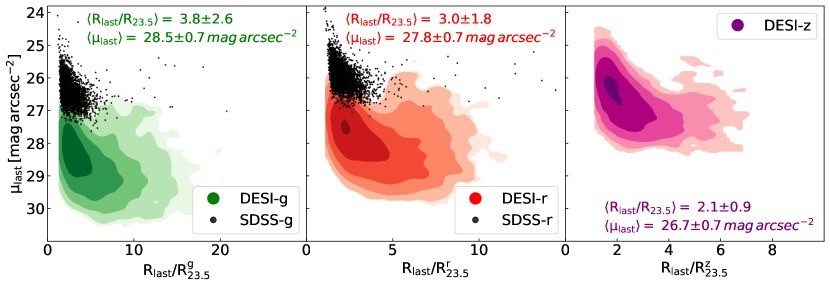
Figure 2: Lowest surface brightness levels and maximal radial extents of DESI surface brightness profiles in the g (left-hand panel), r (center panel) and z-bands (right-hand panel) with coloured contours in log density versus similar quantities for SDSS surface brightness profiles (black dots in the $g$ and $r$ bands; the $z$ band is unavailable) for the same MaNGA galaxies. The radial axis shows the extent of the last point in each surface brightness profile scaled in units of R_23.5. The text within each panel indicates the average depth of our DESI photometry in the radius and surface brightness.

Figure 2 offers a visualization of the greater depth of the DESI imaging (coloured contours) relative to SDSS (black dots for the $g$ and $r$ bands). The photometric depth is chosen as the point at which a profile reaches an surface brightness error threshold of 0.22 mag arcsec^-2 . As a result, the surface brightness levels are typically $\sim$2 mag arcsec^-2 deeper where $\sim$1.5 mag arcsec^-2 is attributed to the deeper DESI imaging (over SDSS) and $\sim$0.5 mag arcsec^-2 is attributed to the isophote sampling method in AUTOPROF (over XVISTA)

The coloured contours show the surface brightness levels and radial extents at which the surface brightness truncation occurs in the three DESI-grz bands. On average, the DESI photometric solutions extend radially beyond $2(z)-3.8(g)~{}R_{\rm 23.5}$ (greater radial extent at bluer wavelengths) and can reach surface brightness levels as low as 26.7(z) to 28.5(g) ${{{{\rm mag}~{}{\rm arcsec}}^{-2}}}$, with some profiles going down to 30 mag arcsec^-2 . Comparison with the SDSS data (extracted by ourselves using XVISTA procedures) shows that the combination of DESI images and the AUTOPROF surface brightness extraction yields profiles that reach typically ${\sim}2~{}{{{{\rm mag}~{}{\rm arcsec}}^{-2}}}$ deeper than SDSS analysed with XVISTA given the same surface brightness uncertainty.

2.2 Parameter Extraction

We briefly describe the parameters inferred from optical and MIR imaging presented in the photometric and environment catalogues. A complete listing of our extracted parameters and their units is given in Table 3 and 4.

2.2.1 Sizes

Some galaxy sizes are calculated relative to total light or measured at different isophotal levels. Relative sizes are calculated at 20, 50, and 80 per cent of the total light. The errors on these sizes are calculated by standard error propagation from the curve of growth (COG). Isophotal sizes are measured at the $\rm 22.5$, $\rm 23.5$ and $\rm 25\,{{{{\rm mag}~{}{\rm arcsec}}^{-2}}}$ isophotes from the surface brightness profiles in their respective band. Errors on isophotal sizes are calculated by standard error propagation from the surface brightness profile. While surface brightness errors tend to be larger than COG errors, the relative slope of the profiles results in larger errors for the sizes based on the COG.

The projected sizes $(R)$ extracted from our photometry can be transformed into 3D physical radii ($r$), i.e., $r(R)$, by modelling projection effects. For flat discy stellar systems, the physical and projected radii are interchangeable (e.g. $r(R)\approx R$). For trixial systems, models suggest that $r(R)\approx(4/3)R$ (Hernquist, 1990; Ciotti, 1991; Ouellette et al., 2017). In Section 6, we review the impact of this transformation on galaxy scaling relations such as the size–mass relation.

2.2.2 Brightness, luminosities, and colours

Total apparent magnitudes and total luminosities enclosed within the $R_{\rm 23.5}$ and $R_{\rm 25}$ radii are presented. The colour terms $g-r$, $g-z$ and $r-z$ are evaluated at $R_{\rm 23.5}$ and $R_{\rm 25}$ in the z band.

The ellipticity of the last measured isophote of a galaxy is used as the representative ellipticity of that galaxy on the sky.

These quantities are all calculated using linear interpolations of consecutive surface brightness profile or curve of growth data. If an interpolation is not possible, the last 25 percent of the profile is used to extrapolate up to that point using a linear fit. A flag for each structural parameter indicates an interpolation or extrapolation.

2.2.3 Concentration

The concentration of light, $C_{\rm 28}$, is a ratio of radii that enclose 20 per cent and 80 per cent of the total light:

$$C_{28}=5\log(R_{80}/R_{20}).$$ (1)

A second measure of concentration, $C_{\rm 25}$, is also presented. Its use of $R_{\rm 20}$ and $R_{\rm 50}$ is operationally similar to Eq. (1). $\rm R_{\rm 50}$ is the effective radius, equivalent to $R_{\rm eff}$.

2.2.4 Stellar mass and surface stellar density

Stellar masses can be inferred from observed colours using stellar mass-to-light colour relations (MLCRs;Courteau et al. 2014). We use five different stellar mass estimates from the MLCRs presented in Roediger & Courteau (2015, hereafter RC15), Zhang et al. (2017, hereafter Z17), and García-Benito et al. (2019, hereafter B19). These MLCRs differ in their choice of stellar population synthesis model, adopted galactic extinctions, and input data used to calibrate the MLCR (global vs. resolved SED fits ). Our stellar mass estimates use $g-r$ and $g-z$ colours measured at R_23.5 in the DESI-z band. The use of multiple colours yields better constraints on mass-to-light ratios (RC15, Z17, Gilhuly & Courteau 2018). The mass-to-light ratios ($\rm\Upsilon_{*}$) calculated from these colours are multiplied by the luminosity in the g, r, and z bands measured at R_23.5, which itself is inferred in the DESI-z band. This results in 30 stellar mass estimates that are averaged to provide a stellar mass estimate used throughout this study. The error in the stellar mass is the standard deviation of the 30 stellar mass measurements. MLCRs in RC15 and Z17 have only been calibrated for late-type systems and are exclusively applied to those systems. The stellar mass measurements for ETGs are thus measured using the MLCR presented in B19.

The stellar $\rm\Upsilon_{*}$ enable the direct conversion of COGs into stellar surface density profiles. We calculate the stellar surface density within 1 kpc ($\Sigma_{1}=M_{\rm*,1kpc}/\pi$) and the effective radius ($\Sigma_{\rm eff}=M_{*}/\pi R_{\rm eff}^{2}$) where $M_{*}$ is the total stellar mass of the galaxy and $\rm M_{\rm*,1kpc}$ is the stellar mass within the 1 kpc aperture.

The MIR stellar masses derived from ${\it W1}-W2$ colours and the MLCR of Cluver et al. (2014) are shown as follows:

$$\log(M_{*}/L_{{\it W1}})=-0.17-2.54\times({\it W1}-W2),$$ (2)

where $L_{{\it W1}}=10^{-0.4(M_{{\it W1}}-M_{\odot,{\it W1}})}$ is the luminosity, $M_{{\it W1}}$ is the absolute magnitude in the ${\it W1}$ filter, and $M_{\odot,{\it W1}}=3.24$ is the absolute magnitude of the Sun in ${\it W1}$ band. The same expression is used to get the luminosity for the WISE $W2$ photometric band, except that $M_{\odot,W2}=3.27$.

These MLCRs use a Chabrier IMF, star formation and AGN activity, dust content, old stellar content, along with detailed stellar mass calibrations (Taylor et al., 2011). The colour in eq. (2) is limited to the range $-0.05\leq({\it W1}-W2)\leq 0.2$ as redder (bluer) sources may be contaminated by AGN or starburst activity (Jarrett et al., 2013).

2.2.5 Environmental parameters

Various environmental properties for 3207 MaNGA galaxies are presented in Table 4. The number of neighbours is extracted from the modified catalogue of Wilman et al. (2010) based on SDSS-DR7 (Abazajian et al., 2009). Galaxies are counted as neighbours if they fall within projected circular apertures of varying radii (0.25-3.0 Mpc) and their heliocentric Hubble flow velocities are within $\pm$1500 km s^-1 of each other.

Central and satellite galaxies are identified via a stellar mass rank with a cylindrical aperture. The radius of the cylindrical aperture depends on the stellar mass of the galaxy and the depth of the cylinder is taken to be $\pm$ 2000 km s^-1. A galaxy with a stellar mass rank of 1 is identified as a central galaxy, whereas a mass rank greater than 1 is associated with a satellite galaxy. See Fossati et al. (2015) and Arora et al. (2019) for a description of the stellar mass rank scheme to identify centrals and satellites. We have also cross-correlated the SDSS and MaNGA catalogues to compute the probability a galaxy being central or satellite according to the scheme of Fossati et al. (2017).

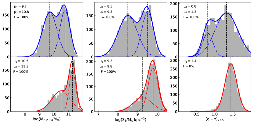
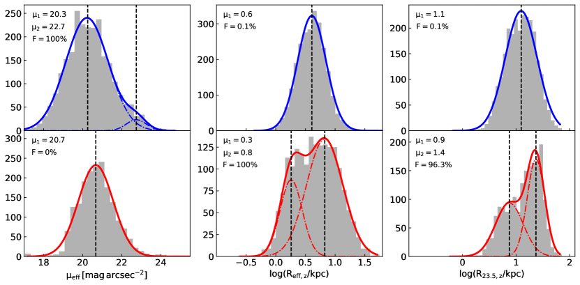
Figure 3: Distribution of MaNGA galaxy properties separated by galaxy morphology; LTGs in blue and ETGs in red. Shown are the stellar mass ($M_{*,23.5}$), stellar mass surface density within 1 kpc ($\Sigma_{1}$), colour measured within $R_{\rm 23.5}$ ($(g-z)_{23.5}$), effective surface brightness ($\mu_{\rm eff}$), effective radius ($R_{\rm eff}$), and isophotal radius at 23.5 mag arcsec^-2 ($R_{\rm 23.5}$). The grey histogram in each panel shows the underlying data distribution. Each LTG/ETG property is fit with a double or single Gaussian; the optimal distribution is determined via the F-test (see the text for details). The data in each panel give the Gaussian mean(s) of the unimodal (bimodal) distributions and the F-test confidence for a single vs. double Gaussian distribution.

2.3 Parameter corrections

Our apparent magnitudes are corrected for Galactic extinction ($A_{\rm g}$), geometric projections ($\gamma$), internal extinction ($A_{\rm i}$), and k-correction ($A_{\rm k}$). Using the following transformation in each band:

$$m_{{\rm corr},\lambda}=m_{{\rm obs},\lambda}-A_{{\rm g},\lambda}-A_{\gamma,\lambda}-A_{{\rm k},\lambda},$$ (3)

the Galactic extinction ($A_{\rm g}$) is obtained from the NSA-Sloan Atlas (NSA; Blanton et al., 2011), which are themselves taken from Schlegel et al. (1998). The cosmological k-correction ($A_{\rm k}$) uses the template from Blanton & Roweis (2007).

Correcting for internal extinction and geometric projections is more challenging, and depends on morphological type. Note that the discussion below applies to late-type galaxies (LTGs); ETGs are assumed dust-free and trixial and no such corrections are applied. MaNGA LTGs are identified via the MaNGA Deep Learning Morphological VAC (MDLM-VAC; Domínguez Sánchez et al., 2018). The effects of projection on the sky bias the measurement of intrinsic properties, hence our attempt to recover face-on equivalent measures with a simple model (Holmberg, 1958; Stone et al., 2021). A common correction for the deprojection of structural parameters involves a linear fit between the desired projected variable and the log of the cosine of the inclination (Giovanelli et al., 1994). This method is expressed in Eq. (4):

$$\log X_{0}=\log X_{i}+\gamma\log(\cos(i)),$$ (4)

where $X_{0}$ is the variable corrected to face-on, $X_{i}$ is the observed measurement, $i$ is the inclination of the galaxy on the sky corrected for the stellar disc thickness and calculated using eq. (5), and $\gamma$ is the fitted correction factor:

$$\cos^{2}i=\frac{(b/a)^{2}-q_{0}^{2}}{1-q_{0}^{2}};\quad(q_{0}=0.13).$$ (5)

These corrections can be performed on a complete sample (Masters et al., 2010) or applied to subsamples based on galaxy properties for which inclination corrections are robust and known such as HI line widths (Tully et al., 1998), galaxy morphology (Maller et al., 2009; Masters et al., 2010), or total infrared luminosity (Devour & Bell, 2019). The correction factor, $\gamma$, encompasses effects due to geometry (line-of-sight projection), stellar populations, and dust extinction as a function of inclination.

T-Type	N	$R_{23.5,g}$	$R_{23.5,r}$	$R_{23.5,z}$	$L_{23.5,g}$	$L_{23.5,r}$	$L_{23.5,z}$	$(g-r)_{23.5}$	$(g-z)_{23.5}$	$\log\Sigma_{1}$
(1)	(2)	(3)	(4)	(5)	(6)	(7)	(8)	(9)	(10)	(11)
0–10	1907	$0.28\pm 0.03$	$0.25\pm 0.03$	$0.23\pm 0.03$	$-0.34\pm 0.08$	$-0.24\pm 0.09$	$-0.12\pm 0.09$	$0.22\pm 0.02$	$0.51\pm 0.04$	$\phantom{-}0.01\pm 0.08$
0–3	829	$0.38\pm 0.05$	$0.37\pm 0.05$	$0.35\pm 0.05$	$-0.05\pm 0.11$	$\phantom{-}0.10\pm 0.12$	$\phantom{-}0.25\pm 0.12$	$0.34\pm 0.03$	$0.72\pm 0.04$	$\phantom{-}0.43\pm 0.11$
4–5	958	$0.21\pm 0.04$	$0.19\pm 0.04$	$0.18\pm 0.04$	$-0.42\pm 0.11$	$-0.28\pm 0.11$	$-0.15\pm 0.11$	$0.26\pm 0.02$	$0.62\pm 0.04$	$\phantom{-}0.05\pm 0.11$
6–10	164	$0.31\pm 0.08$	$0.26\pm 0.08$	$0.22\pm 0.08$	$-0.28\pm 0.23$	$-0.28\pm 0.24$	$-0.08\pm 0.24$	$0.01\pm 0.03$	$0.09\pm 0.08$	$-0.25\pm 0.18$

Table 1: Inclination correction terms, $\gamma$, for various galaxy structural parameters in different photometry bands. Column (1) shows the T-Type bins used for the correction; column (2) presents the number of data points used for the fitting; and columns (3)–(11) show the correction factors for different structural properties. The first row gives $\gamma$ for all galaxies; the next three rows give $\gamma$ for specific morphological bins.

We solve Eq. (4) for $\gamma$ with a forward least-squares fit between the desired variable and $\cos(i)$ in log space. For the fitting, we restrict the sample to an inclination range of $30^{\circ}<i<80^{\circ}$ and assume an intrinsic thickness of $q_{0}=0.13$ to convert the ellipticity to inclination (Hall et al., 2012; Ouellette et al., 2017). Errors on $\gamma$ are calculated using bootstrap sampling. Table 1 tabulates the correction factor, $\gamma$, for various galaxy structural properties of the MaNGA LTG sample in the grz bands. We present $\gamma$ for the full sample (first row of Table 1) and split into three morphological bins done using the MLDM-VAC (last three rows of Table 1).

The absolute value of these correction factors differ from those presented in Masters et al. (2010) and Stone et al. (2021). However, in all cases, the correction factors are small. For example, the correction factor for an isophotal radius in the transparent case is $\gamma\approx 2.3$ (Giovanelli et al., 1994), compared to our correction factor of $\rm{\sim}0.25\pm 0.02$.

Scaling relation	Uncorrected		Corrected T–Types 1-10		Corrected 3 T-Type bins
	m	$\sigma$	m	$\sigma$	m	$\sigma$
(1)	(2)	(3)	(4)	(5)	(6)	(7)
$\Sigma_{1}$–$M_{\rm*,23.5}$	$0.96\pm 0.01$	$0.24\pm 0.01$	$0.96\pm 0.01$	$0.23\pm 0.01$	$0.96\pm 0.01$	$0.23\pm 0.01$
$R_{23.5,z}$–$M_{*,23.5}$	$0.34\pm 0.01$	$0.11\pm 0.01$	$0.34\pm 0.01$	$0.11\pm 0.01$	$0.35\pm 0.01$	$0.10\pm 0.01$
$R_{23.5,z}$–$\Sigma_{1}$	$0.30\pm 0.01$	$0.17\pm 0.01$	$0.29\pm 0.01$	$0.16\pm 0.01$	$0.30\pm 0.01$	$0.17\pm 0.01$
$R_{23.5,z}$–$L_{23.5,z}$	$0.41\pm 0.01$	$0.08\pm 0.01$	$0.41\pm 0.01$	$0.09\pm 0.01$	$0.41\pm 0.01$	$0.09\pm 0.01$
$\Sigma_{1}$–$L_{23.5,z}$	$0.94\pm 0.01$	$0.30\pm 0.01$	$0.95\pm 0.01$	$0.30\pm 0.01$	$0.93\pm 0.01$	$0.29\pm 0.01$
$(g-z)_{23.5}$–$L_{23.5,z}$	$0.24\pm 0.01$	$0.24\pm 0.01$	$0.25\pm 0.01$	$0.22\pm 0.01$	$0.22\pm 0.01$	$0.21\pm 0.01$

Table 2: Variation of slopes and scatters of galaxy structural scaling relations due to inclination corrections. Column (1) indicates the scaling relation; columns (2) and (3) give the uncorrected slope and scatter; columns (4) and (5) give the slope and scatter with a single full-sample correction (all T-Types); columns (6) and (7) give the slopes and scatter with corrections applied to three morphological bins.

Ideally, an accurate inclination correction model should yield a reduction of the observed scatter in various galaxy scaling relations. This concept is tested in Table 2, which presents the variation of the slopes and scatter for a suite of structural galaxy scaling relations with inclination corrections. The slopes and scatter are found to be robust against inclination corrections for nearly all scaling relations presented. A significant variation in the scatter of the $(g-z)_{23.5}--L_{23.5,z}$ relation is found for both inclination correction models, with or without binning by morphology. In light of the null variation in the slopes and scatter of galaxy scaling relations, we apply inclination corrections to our photometry without reducing our sample into various morphological bins.

Column name	Description	Unit	Data yype
MANGA-ID	MaNGA Identification	–	string
PlateIFU	MaNGA Plate-IFU	–	string
ObjID	SDSS-DR15 photometric identification number	–	long int
RA	Object Right Ascension (J2000)	∘	float
DEC	Object Declination (J2000)	∘	float
Z	NSA or SDSS redshift	–	float
TTYPE	Morphological T-Type (from MDLM-VAC)	–	float
GAL_EXTINCTION	Galactic extinction (DESI grz only)	mag	float
KCORRECTION	Cosmological K-Corrections (DESI grz only)	mag	float
R20	Radius where 20 per cent of the total light is integrated	arcsec	float
R20_E	Error in R20	arcsec	float
Reff	Effective radius	arcsec	float
Reff_E	Error in effective radius	arcsec	float
R80	Radius where 80 per cent of the total light is integrated	arcsec	float
R80_E	Error in R80	arcsec	float
R22.5	Isophotal radius calculated at $\rm 22.5\,{{{{\rm mag}~{}{\rm arcsec}}^{-2}}}$	arcsec	float
R22.5_E	Error in R22.5	arcsec	float
R22.5_FLAG	Method of calculation: interpolation (0) and extrapolation (1)	boolean	int
R23.5	Isophotal radius calculated at $\rm 23.5\,{{{{\rm mag}~{}{\rm arcsec}}^{-2}}}$	arcsec	float
R23.5_E	Error in R23.5	arcsec	float
R23.5_FLAG	Method of calculation: interpolation (0) and extrapolation (1)	boolean	int
R25	Isophotal radius calculated at $\rm 25\,{{{{\rm mag}~{}{\rm arcsec}}^{-2}}}$	arcsec	float
R25_E	Error in R25	arcsec	float
R25_FLAG	Method of calculation: interpolation (0) and extrapolation (1)	boolean	int
C25	Concentration index measured using R20 and Reff	–	float
C28	Concentration index measured using R20 and R80	–	float
MU_20	Surface brightness at R20	${{{{\rm mag}~{}{\rm arcsec}}^{-2}}}$	float
MU_20_E	Error in Mu_20	${{{{\rm mag}~{}{\rm arcsec}}^{-2}}}$	float
MU_20_FLAG	Method of calculation: interpolation (0) and extrapolation (1)	boolean	int
MU_EFF	Surface brightness at the effective radius	${{{{\rm mag}~{}{\rm arcsec}}^{-2}}}$	float
MU_EFF_E	Error in effective surface brightness	${{{{\rm mag}~{}{\rm arcsec}}^{-2}}}$	float
Mu_EFF_FLAG	Method of calculation: interpolation (0) and extrapolation (1)	boolean	int
MU_80	Surface brightness at R80	${{{{\rm mag}~{}{\rm arcsec}}^{-2}}}$	float
MU_80_FLAG	Error in Mu_80	${{{{\rm mag}~{}{\rm arcsec}}^{-2}}}$	float
MU_80_FLAG	Method of calculation: interpolation (0) and extrapolation (1)	boolean	int
MAG23.5	Total apparent magnitude within R23.5	mag	float
MAG23.5_E	Error in total apparent magnitude within R23.5	mag	float
MAG23.5_FLAG	Method of calculation: interpolation (0) and extrapolation (1)	boolean	int
MAG25	Total apparent magnitude within R25	mag	float
MAG25_E	Error in total apparent magnitude within R25	mag	float
MAG25_FLAG	Method of calculation: interpolation (0) and extrapolation (1)	boolean	int
L23.5	Total luminosity within R23.5	$L_{\odot}$	float
L25	Total luminosity within R25	$L_{\odot}$	float
ELLIPTICITY	Ellipticity of the last isophote; $1-(b/a)$	–	float
PA	Position angle of the last isophote measured from north to east (DESI grz only)	∘	float
MSTAR_235	Stellar mass measured at the z-band R23.5 (z & W1 band only)	$\rm M_{\odot}$	float
MSTAR_235_E	Error in stellar mass estimates measured at z band R23.5 (z band only)	$\rm M_{\odot}$	float
MSTAR_25	Stellar Mass measured at the z-band R25 (z band only)	$\rm M_{\odot}$	float
MSTAR_25_E	Error in stellar mass estimates measured at z-band R25 (z band only)	$\rm M_{\odot}$	float
SIGMA1	Stellar mass surface density within 1 kpc (z band only)	$\rm M_{\odot}\,kpc^{-2}$	float
SIGMA1_E	Error in SIGMA1 (z band only)	$\rm M_{\odot}\,kpc^{-2}$	float
SIGMA_EFF	Stellar mass surface density within Reff (z band only)	$\rm M_{\odot}\,kpc^{-2}$	float
SIGMA1_EFF_E	Error in SIGMA_EFF (z band only)	$\rm M_{\odot}\,kpc^{-2}$	float
COLOR	$g-r$ and $g-z$ measured at z-band R23.5 and R25 (z band only)	mag	float

Table 3: Photometric quantities for the MaNGA DESI photometric catalogue. The table includes calculated parameters along with the units and the data types. All parameters presented are uncorrected for Galactic extinction, inclination and cosmology. These parameters are available in three separate files for the DESI grz bands. The three full tables are presented as supplementary material.

Column Name	Description	Unit	Data type
MANGA-ID	MaNGA Identification	–	string
PlateIFU	MaNGA Plate-IFU	–	string
ObjID	SDSS-DR15 photometric identification number	–	long int
RA	Object Right Ascension (J2000)	∘	float
DEC	Object Declination (J2000)	∘	float
Z	NSA or SDSS redshift	count	float
Dens_01	Number of neighbours within a 0.1-Mpc aperture	count	int
Dens_02	Number of neighbours within a 0.2-Mpc aperture	count	int
Dens_05	Number of neighbours within a 0.5-Mpc aperture	count	int
Dens_1	Number of neighbours within a 1-Mpc aperture	count	int
Dens_2	Number of neighbours within a 2-Mpc aperture	count	int
Dens_3	Number of neighbours within a 3-Mpc aperture	count	int
Mrank_AA	Identification of central or satellite galaxy; central (1) and satellite (>1)	rank	int
P_CEN	Probability of the galaxy being the central member in the halo	rank	float
P_SAT	Probability of the galaxy being a satellite in the halo	–	float

Table 4: Environmental properties for the MaNGA galaxies. The table includes each parameter along with the units and data types. The full table is presented as supplementary material.

3 Parameters Distributions

This section provides an overview of some important MaNGA galaxy properties and their range. Figure 3 offers a broad appreciation of the distribution of structural properties for galaxies in the MaNGA public release. For instance, if dwarf galaxies are defined as having a stellar mass $\log(M_{*}/M_{\odot})\leq 9.5$ (Woo et al., 2008; Ouellette et al., 2017), only 11 percent of our galaxies are dwarfs. Our results in this section clearly highlight the presence of distinct populations in each of the LTG and ETG categories. The latter is made clear through the unimodal and bimodal trends displayed by some structural and dynamical parameters (Tully & Verheijen, 1997; McDonald et al., 2009; Sorce et al., 2013; Ouellette et al., 2017). We define a unimodal distribution as one described by a normal distribution. The figure of merit to distinguish a bimodal from a unimodal distribution is the F-test that gives the probability that the observed distributions originate from two distinct Gaussian populations rather than a single one. These populations are represented by single or double Gaussian fits in Figure 3. F-test confidence results for a double vs a single Gaussian distribution and the fitted means for the double/single population(s) are indicated in each panel. Unimodal distributions are found for LTG sizes (effective and isophotal) and ETG effective surface brightnesses and colour.

The following properties for LTGs show bimodal signatures; stellar mass (top left-hand panel), stellar surface density with 1 kpc (middle panel), effective surface brightness (bottom left-hand) and colour (top right-hand) measured at 23.5 mag arcsec^-2 . The notion of surface brightness bimodalities has been addressed at some length in (Ouellette et al., 2017, and references therein). Surface brightness bimodalities in LTGs are especially conspicuous at dust-insensitive wavelengths such as the z band (Sorce et al., 2013).

For ETGs, stellar mass, stellar surface density within 1 kpc, isophotal radius at 23.5 mag arcsec^-2 , and effective radius show bimodal signatures. A bimodality in the galaxian properties shown here reflects environmental influences, varying merger and star formation histories, and different radial dark matter fractions, which all play a key role in galaxy evolution. The coupling of these structural bimodalities with bimodal dynamical properties (if any) would greatly enhance galaxy formation scenarios.

The detailed investigation of bimodal trends in scaling relations, and the identification of galaxy subclasses, will be presented elsewhere. For now, we appreciate the need to consider one or two populations in fitting scaling relations over a range of galaxian properties.

4 Literature Comparisons

The following section presents comparisons of our galaxy structural parameters with similar values found in the literature. We first present a multifaceted comparison of the 1D surface brightness profiles generated using model-independent (e.g. AUTOPROF , XVISTA) and model-dependent (e.g. GALFIT, PYMORPH ) methods. Effective (half-light), isophotal radii and apparent magnitudes from the MPP-VAC of F19 are also compared with our photometry. This comparison recognizes that the MPP-VAC reports parameters from circularized light profiles. We caution that this operation is especially uncertain in light of unknown dust distributions, non-axisymmetric feature and disc thicknesses, and the vagaries of 2D image decompositions (Gilhuly & Courteau, 2018). Total magnitudes, and effective radii, should be the least model-biased parameters from F19, and hence our comparison below. Stellar masses are also compared with a PCA-based stellar mass estimation technique from Pace et al. (2019, hereafter P19). For the sake of comparison, parameters presented in this section are not corrected for Galactic extinction, inclination, and cosmology.

4.1 Surface brightness profile comparisons

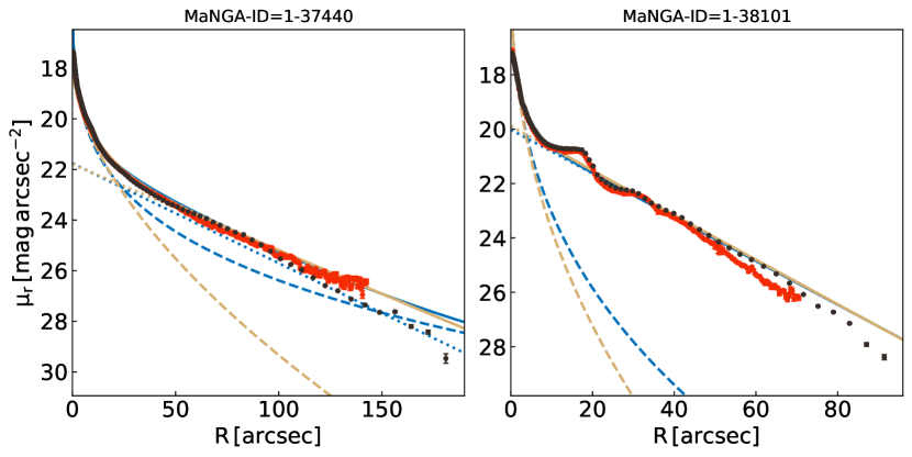
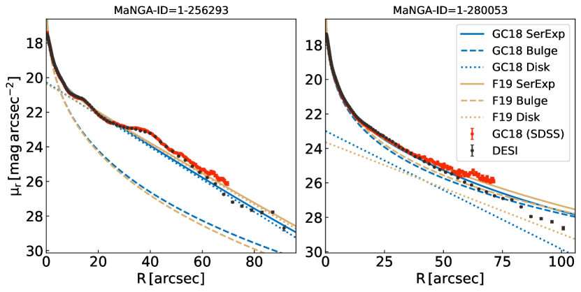
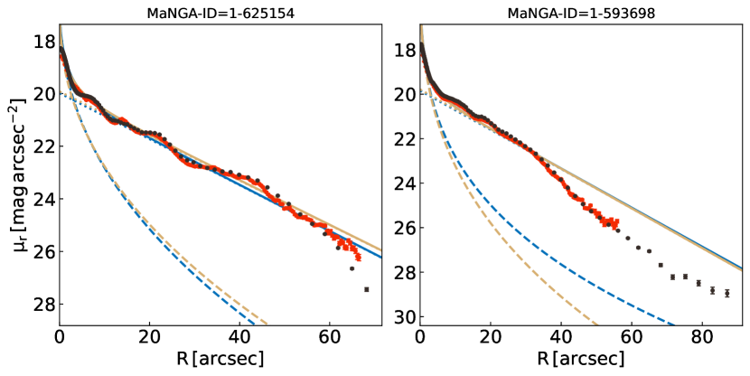
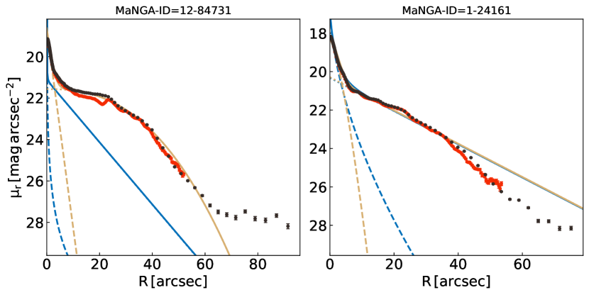
Figure 4: Comparison of our DESI-based 1D r-band surface brightness profile (black dots) with the SDSS-based surface brightness profile (red dot) of GC18. Also compared are the 2D Sérsic + Exponential decompositions using GALFIT by GC18 (cyan solid lines) and F19 (gold solid line). The Sérsic + Exponential decompositions are separated by their respective bulge (dashed line) and disc (solid line) contributions. Missing coloured lines represent failed fits by the original authors.

Figure 4 compares 1D r-band surface brightness profiles extracted from DESI images (black points) by us and from SDSS images by GC18 (red points). The excellent agreement between those profiles results from quality DESI/SDSS imaging and the robust non-parametric surface brightness profile extraction with XVISTA and AUTOPROF . Figs. 1 and 4 compare various global properties between XVISTA and AUTOPROF , showing that both codes reproduce local variations in 1D surface brightness profiles with high fidelity.

Our catalogue also overlaps with F19 and GC18. The latter two studies used the 2D image fitting algorithm GALFIT to obtain Bulge-Disc decompositions for their samples based on the MaNGA and CALIFA samples, respectively. A total of 16 galaxies overlap between the MaNGA (us and F19) and CALIFA (GC18) samples. These overlapping galaxies enable a comparison of our independent results.

In Figure 4, the blue and gold solid line show the Sérsic + Exponential decompositions by Gilhuly & Courteau (2018) and F19 respectively, for eight galaxies using GALFIT. We caution that the MPP-VAC (F19) present total apparent magnitudes in the circularized plane of the galaxy, i.e. corrected to face-on based on the simplest assumptions of a dust-free, infinitesimally-thin disc. The recovery of total apparent magnitudes ($m$) from the MPP-VAC in the plane of the sky must therefore be made with the equation $(m_{r}^{\prime}=m_{r}+2.5\log(b/a))$ for the bulge and disc components, where $b/a$ is the axis ratio of the galaxy.

The appreciation of more complex disc systems, with their triaxial bulges, thicker mid-planes, and sporadic dust extinction, calls for a more extensive modelling. Stone et al. (2021) performed an extensive analysis of inclination corrections for disc galaxies. While some correction models showed a scatter reduction of various galaxy scaling relations, little agreement between different correction models was found.

For six out of the eight galaxies, the two independent GALFIT decompositions return Sérsic + Exponential models that can differ by as much as ${\sim}0.4\,{{{{\rm mag}~{}{\rm arcsec}}^{-2}}}$, demonstrating the great subjectivity between these model-dependent solutions while our non-parametric comparison only show differences on the order of ${\sim}0.09\,{{{{\rm mag}~{}{\rm arcsec}}^{-2}}}$. In some cases, only one user can find a valid solution for the GALFIT decomposition. Where both fits converge, they often find different bulge to disc ratios with a difference of ${\sim}0.3$ dex. Similar caveats for Bulge-Disc decompositions for the same galaxies using two different image fitters (GALFIT and IMFIT (Erwin, 2015)) by GC18 showed discrepant results as well.

The large variations between the solutions of GC18 and F19, as well as the analysis presented in GC18, remind us that generic parametric solutions are especially fragile and inconclusive. For these reasons, an analysis of galaxy structure or scaling relation should rely on the non-parametric characterization of surface brightness profiles.

4.2 Effective sizes

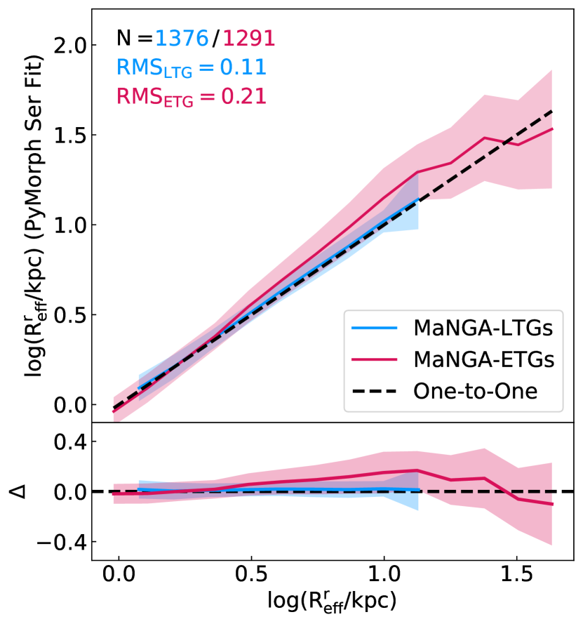
Figure 5: Comparison of our model-independent effective radii from DESI r-band surface brightness profiles with those from a single Sérsic fit from F19. The solid lines show the median for MaNGA-LTGs (blue) and MaNGA-ETGs (red) and the shaded region shows the scatter within a bin of size 0.12 dex. The dashed line shows the one-to-one line. The inset text shows the number of data points and root mean square (rms) for the LTG and ETG populations. The bottom panel shows the residual $\Delta=\log(R^{r}_{\rm eff}[PYMORPH]/R^{r}_{\rm eff})$.

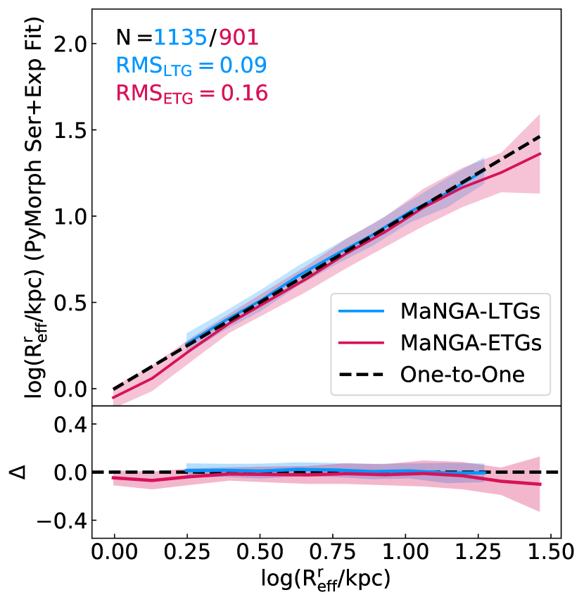
Figure 6: Same as Figure 5 but the y-axis uses effective radii from Sérsic and exponential fits by F19.

Figure 5 compares our non-parametric $R_{\rm eff}$, measured in the DESI r band, with those found in F19 for a single Sérsic fit with PyMorph. We have used the MDLM-VAC to divide our sample into LTG and ETG categories. Size measurements are taken in the $r$-band to enable a direct comparison with PyMorph results. PYMORPH and AUTOPROF agree well at small radii; at larger radii AUTOPROF yields smaller sizes than PYMORPH .

This behaviour is expected as a single Sérsic fit does not capture all the light from the outer regions of a galaxy, with low S/N, yielding a larger estimate for $R_{\rm eff}$. The effect is amplified for larger PYMORPH $R_{\rm eff}$ and for the ETG sample due to their higher light concentration relative to LTGs. For the complete population, a single Sérsic fit from F19 results in larger effective radii by 0.21 dex compared to our results.

The agreement between our methods improves with the two-component fits from F19. Figure 6 shows a comparison between our non-parametric effective radii and those extracted from two-component Sérsic exponential fits. Both ETGs and LTGs are in agreement, though at large radii the scatter increases.

While the PYMORPH two-component fit improves the overall agreement with AUTOPROF , there remains significant random variations, especially with quantities determined relative to the total light of the galaxy, like the effective radius, $R_{\rm eff}$. The latter suffered from poor reproducibility, largely due to the uncertain definition of total apparent magnitude of a galaxy. In a similar vein, Hall et al. (2012) found that the scatter of velocity–radius–luminosity (VRL) scaling relations is reduced with isophotal radii and Trujillo et al. (2020) found that a stellar mass density radius reduces scatter in the size–mass relation. Similar impressions were echoed by GC18 who found differences as large as 0.16 dex (45%) between non-parametric and model-dependent measures of $R_{\rm eff}$ for CALIFA galaxies (Walcher et al., 2014). González-Samaniego et al. (2017) also used the FIRE simulations to point out the same pathology about $R_{\rm eff}$. For the size-dependent analyses that follow (Section 6), we limit our use of effective radii and pay special attention to isophotal size metrics. The scatter in the size–mass relation is discussed in Section 6.

4.3 Isophotal sizes

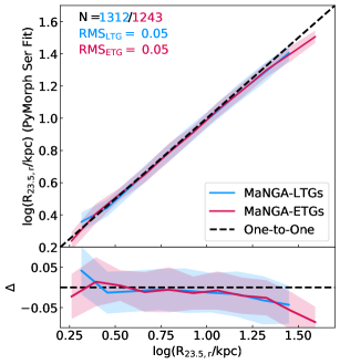
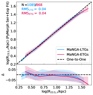
Figure 7: Comparison of our model-independent isophotal radius measured at $23.5$ mag arcsec^-2 from DESI r-band surface brightness profiles with model-dependent PYMORPH decomposition from F19. The solid lines show the median for MaNGA-LTGs (blue) and MaNGA-ETGs (red), and the shaded region shows the scatter in a bin of width 0.12 dex. The dashed line is the one-to-one line. The legend shows the number of data points and rms for the LTG and ETG populations. The left- and right-hand panels show the Sérsic and Sérsic+Exponential fits, respectively. The bottom panels show the residual $\Delta=\log(R^{r}_{23.5}[PYMORPH]/R^{r}_{23.5})$.

The parameters from the MPP-VAC can be used to construct de-projected surface brightness profiles in order to infer the isophotal radii measured at $23.5$ mag arcsec^-2 . These are compared with matching size measurements from the DESI photometry in Figure 7. Disagreements in isophotal sizes are larger for galaxies with preferred Sérsic model (${\sim}0.05\,$dex) compared to galaxies with preferred Sérsic+Exponential model (${\sim}0.04\,$dex). This reaffirms the results from Section 4.2 that simple Sérsic models cannot account for all of the galaxy light.

The comparison of model-independent isophotal radii measured with XVISTA and AUTOPROF in Figure 1 showed more consistency ($0.02\,$dex), indicating that non-parametric modelling of galaxies is more reproducible. The larger rms ($\sim$0.05 dex) is explained by the vagaries in parametric modelling from GALFIT. Comparing Figure 7 and Figure 6 demonstrates that that isophotal sizes ($R_{\rm 23.5}$) are more consistent than sizes based on fraction of total light even while comparing non-parametric with model-dependent sizes.

4.4 Apparent magnitudes

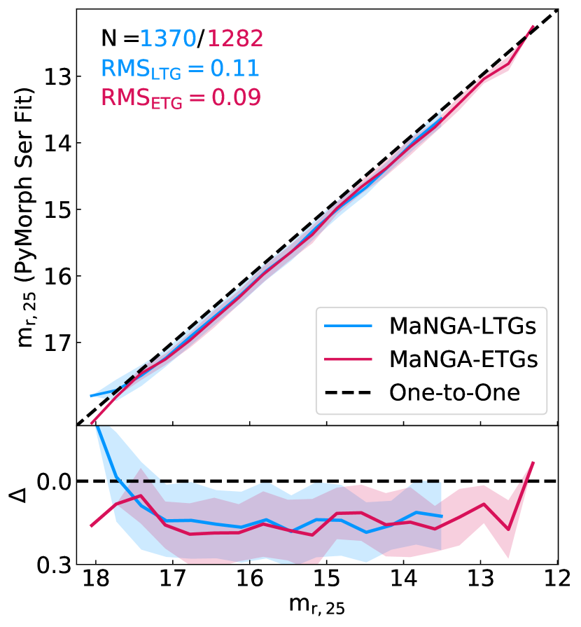
Figure 8: Comparison of our model-independent apparent magnitudes from DESI r-band surface brightness profiles with those from a single Sérsic fit from F19. For both methods, the total apparent magnitude is measured within the $25\,{{{{\rm mag}~{}{\rm arcsec}}^{-2}}}$ isophote. The bottom panel shows the residual.

Next, total apparent magnitudes extracted from DESI photometry are compared with MPP-VAC magnitudes from F19. The total apparent magnitudes are both calculated within $25\,{{{{\rm mag}~{}{\rm arcsec}}^{-2}}}$ and are not corrected for cosmology, Galactic and inclination extinctions. While total magnitudes are here mostly reported at the $23.5\,{{{{\rm mag}~{}{\rm arcsec}}^{-2}}}$ levels to maximize comparisons with literature values, the current comparisons (Figure 8 and 9) at the $25\,{{{{\rm mag}~{}{\rm arcsec}}^{-2}}}$ isophotal level takes advantage of the superior DESI imaging depth. Once again, the F19 total apparent magnitudes are deprojected according to the expression, $m^{\prime}=m+2.5\log(b/a)$. Figure 8 compares apparent r-band magnitudes from our DESI surface brightness profiles with Sérsic fit magnitudes from F19, in various galaxy morphological bins. The rms values are given in dex (magnitude divided by 2.5). For both ETGs and LTGS, the DESI surface brightness profiles from AUTOPROF are $\sim 0.10$ dex brighter than those from PYMORPH with a Sérsic fit. This further highlights that a single Sérsic fit fails to capture all the light from the object, leading to disagreements in effective galaxy sizes (Section 4.2).

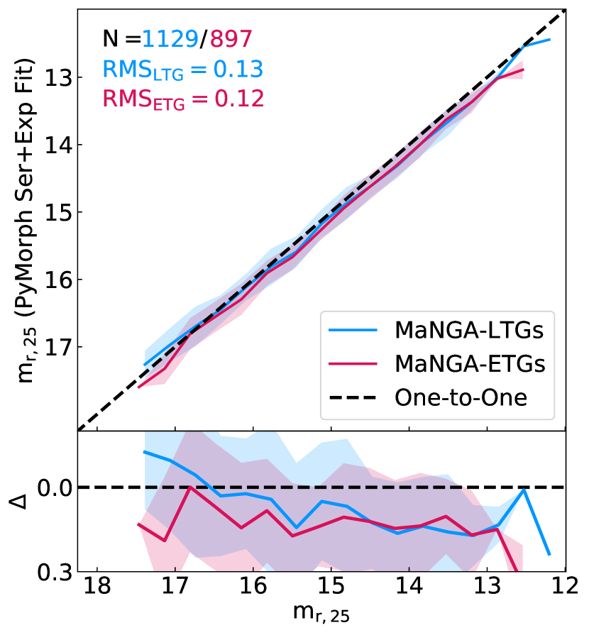
Figure 9: Same as Figure 8 with apparent magnitude on the y-axis for a double Sérsic and exponential fit from F19.

.

Surprisingly, the addition of a second, exponential, component in PYMORPH for MaNGA galaxies results in poorer fits (Figure 9). While random variations between PYMORPH and AUTOPROF for LTGs are reduced with an additional component, PyMorph still underestimates the total light (calculated using the analytic Sérsic function) relative to our analysis. The shaded regions for both LTGs and ETGs in Figure 9 represent the inter-quartile range of the residuals. With our large sample, we can estimate the random error (as $1/\sqrt{N}\sim 0.03\,$dex) to be very small, and the rms errors are thus largely systematic. Indeed, disagreements with our apparent magnitudes emerge largely from the model-dependent nature of the F19 photometric analysis that do not account for non-axisymmetric features such as bars, rings and spiral arms. Features unaccounted for by PYMORPH will systematically yield fainter total magnitudes relative to non-parametric estimates. Along with the surface brightness profile comparison in Section 4.1, the size and apparent magnitude comparisons further reinforce the benefits of using model-independent technique for measuring galaxy structural properties.

4.5 Stellar masses

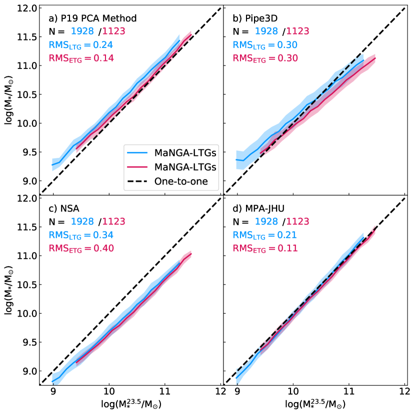
Figure 10: Comparisons of our stellar mass estimates from DESI photometry measured within $\rm R_{23.5,z}$ shown on the x-axis versus those from various literature sources. The y-axes compare stellar mass estimates from panel (a): P19; panel (b): Pipe3D (Sánchez et al., 2016); panel (c): NSA photometry (Blanton & Roweis, 2007); and panel (d) the MPA-JHU catalogue (Kauffmann et al., 2003; Brinchmann et al., 2004). The colour scheme matches that of Figure 5. The solid line shows the median trends and the shaded regions represent the scatter within a bin. The top left inset gives the number of LTG (blue) and ETG (red) galaxies, as well as the rms for the respective stellar mass differences.

Figure 10 presents a comparison of our stellar mass estimates on the x-axis versus various literature sources on the y-axis. Our stellar masses are an amalgam of 30 variants derived from optical MLCRs (RC15; Z17; B19). These MLCRs use stellar population synthesis (SPS) models from Bruzual & Charlot (2003, hereafter BC03) and Conroy & Gunn (2010). The MLCRs presented in B19 apply to all galaxy morphologies, while RC15 and Z17 were only calibrated for LTGs and are here only used for those systems. The stellar masses from P19 in panel (a) were derived using $\Upsilon_{*}$ ratios calculated with a principal component analysis (PCA) that finds the best-fitting synthetic spectra for each MaNGA spaxel observation. Our stellar masses are measured within $R_{\rm 23.5}$ in the z band, while those from P19 are calculated using the footprint of the MaNGA IFU with aperture correction performed using NSA excess fluxes.

The aperture-corrected stellar masses from P19 appear to be systematically larger than our estimates, especially for MaNGA LTGs (panel a of Figure 10). The comparison yields an rms offset of 0.25 (0.14) dex and a scatter of 0.09 (0.08) for the LTG (ETG) populations. These systematic differences are likely due to the adopted star formation histories (SFHs). P19 adopted smooth SFH templates; the omission of bursts in SFHs can bias the $\Upsilon_{*}$ high (RC15), resulting in larger stellar mass estimates. These systematic effects are more pronounced for LTGs as these systems have more bursty and active star formation histories. However, the reported rms offsets for this comparison are well within the systematic errors expected for MLCRs. Panel (b) compares our stellar masses against those calculated from Pipe3D (Sánchez et al., 2016); these are integrated within the FOV of the MaNGA IFU. We find an even larger rms offset and scatter range than our comparison with P19. The Pipe3D comparison shows a large rms difference of 0.30 dex and a scatter of 0.16 (0.1) dex for the LTGs (ETGs). For both LTGs/ETGs, our stellar mass estimates at the low (high) mass end are smaller (larger) than Pipe3D. The difference between our respective stellar mass estimates may arise from $\Upsilon_{*}$ calculation, which is done pixel by pixel for Pipe3D whereas our $\Upsilon_{*}$ is calculated using a global colour.

Panel (c) in Figure 10 compares stellar mass estimates inferred via K-corrected elliptical Petrosian photometry from the NSA (Blanton & Roweis, 2007). In our stellar mass comparisons, NSA estimates present the largest discrepancy with the our photometry. Sources for this offset include (i) missing flux in the NSA photometry, (ii) adoption of simple stellar populations (SSPs) for the $\Upsilon_{*}$ conversions, and/or (iii) the use of Petrosian magnitudes. The NSA elliptical-Petrosian photometry has been shown to yield bluer colors $(\Delta(g-r)=0.046\pm 0.008)$ that the SDSS photometry for the complete MaNGA sample P19, thus causing systematic differences in stellar mass estimates.

Finally, Panel (d) compares our stellar mass estimates with those from the MPA-JHU catalogue (Brinchmann et al., 2004). Their stellar mass estimates are calculated using the $z$-band stellar $\Upsilon_{*}$ ratio obtained using the SDSS spectra that best model the H$\,\delta$ and D4000 absorption features applied to $z$ band luminosities. The comparison in Panel (d) shows a superb match between the MPA-JHU and our photometry with a median across all bins lying close to the 1:1 line and an rms of 0.23 (0.12) dex for the LTGs (ETGs). Comparing all stellar mass estimates presented in Figure 10, MPA-JHU has the best agreement for both morphological types.

5 MIR Structural Parameters

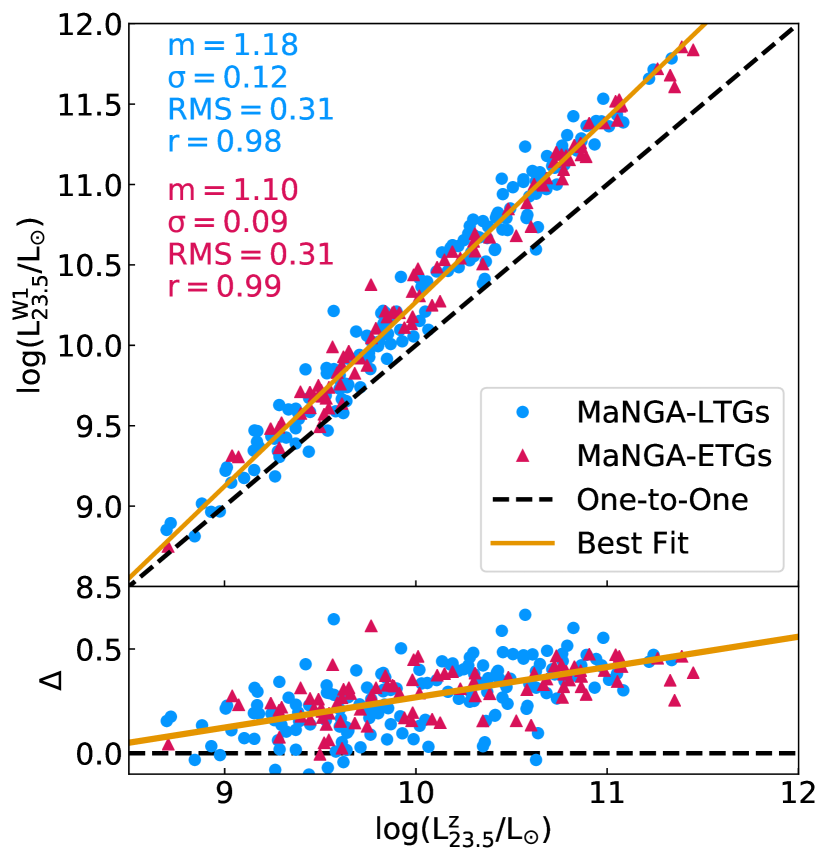
Figure 11: Comparison of total integrated luminosity inferred from DESI and W1 images measured at $R_{23.5,z}$. The blue circles present the MaNGA-LTGs, and red triangles present MaNGA-ETGs. The orange line shows the best fit for the complete population and inset text presents statistics for the two populations.

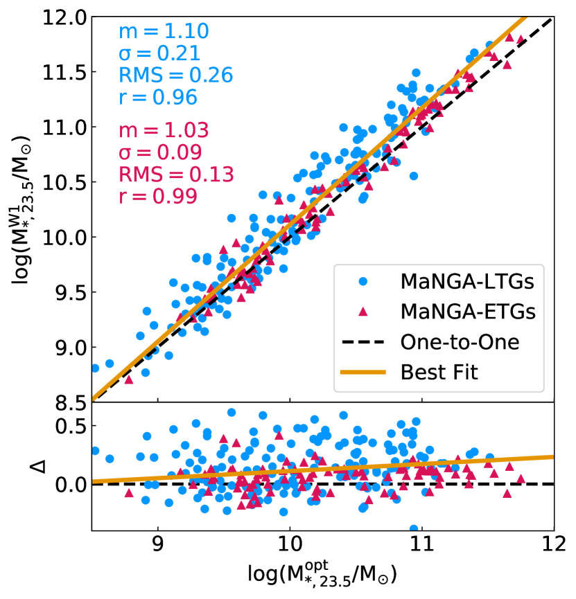
Figure 12: Comparison of stellar masses inferred from DESI and W1 images measured at $R_{23.5,z}$. The format is the same as Figure 11. For LTGs, "opt" stellar masses are an average of five MLCRs presented in Section 2.2.4. For ETGs, "opt" stellar masses are measured using the MLCR of B19.

This section presents a comparison of galaxy structural parameters extracted from our optical and MIR photometry. We first caution that surface brightnesses sampled with different pixel resolutions, as is the case here with the DESI and WISE data, cannot be compared directly unless profiles are all sampled (degraded) to the lowest resolution. Therefore, only integrated quantities between DESI and WISE data are compared below.

Figure 11 shows the W1 and DESI z-band luminosities measured at $R_{23.5,z}$. For the complete sample, W1 luminosities are typically larger than z-band luminosities by $\sim$0.3 dex, as a result of a greater sensitivity of the W1 bandpass to the dominant low mass (older) stellar population and lesser dust extinction in the W1 band. Furthermore, the W1-$z$ colour term grows significantly with luminosity, as seen in the residual panel of Figure 11. The scatter between DESI z and W1 luminosities is tighter for the MaNGA-ETGs (than LTGs) largely due to their star formation activity being quenched (Cluver et al., 2014). The larger scatter for the LTGs population is also indicative of a more diverse stellar population and larger dust content.

Finally, Figure 12 compares stellar masses inferred from optical and MIR photometry measured at $R_{23.5,z}$. As discussed in Section 2.2.4, we used the average of five different MLCRs with $g-r$ and $g-z$ colours to calculate optical stellar masses. Mass estimates of a stellar population should not depend on the flux tracer, however dust extinction in optical bands could lead to systematic offsets, especially in late-type systems. While a systematic offset of 0.21 dex is detected in Figure 12, with W1 stellar masses being larger than optical, the latter is within the bounds of typical MLCRs systematic variations of 0.2-0.3 dex (Taylor et al., 2011; Courteau et al., 2014; Roediger & Courteau, 2015). Our optical and MIR stellar mass measurements are thus in good agreement RC15. This reaffirms the conclusion that optical colours are robust tracers of the stellar mass (Taylor et al., 2011).

The differences in luminosity, and stellar mass (11 and 12 respectively) at different wavelengths can serve as calibrators for stellar population models and numerical models of galaxy formation (MacArthur et al., 2004; Renzini, 2006; Zheng et al., 2020).

6 Galaxy Scaling Relations

In the previous sections, we have demonstrated the robustness of our optical and MIR photometry. We have also shown that our DESI optical photometry is $\sim$1.5 mag arcsec^-2 deeper than nominal SDSS imaging, and we have used the MLDL-VAC to define our MaNGA LTG and ETG subsamples.

We now present, in Table 5, a variety of scaling relations in DESI (g, r, z) and WISE (W1, W2) band passes for our MaNGA data. The scaling relations are all presented as orthogonal linear regressions (Virtanen et al., 2020, SCIPY). This treatment facilitates comparisons with matching studies in the literature, though we note that subtle differences in choice of fitting method and parameter definition can affect the final scaling relation parameters (see Table 6). As discussed in Section 3 and Figure 3 some distributions may call for more complex modelling, such as that characterized by a slowly varying slope or a piece-wise function. We revisit these complexities below.

Below we focus on two popular scaling relations drawn from our DESI and WISE photometric investigations of MaNGA LTGs and ETGs, namely the size–stellar mass ($R-M_{*}$) and $\Sigma_{1}$–stellar mass ($\Sigma_{1}$-M_∗) relations. In the following sections, all structural parameters are measured at R_23.5 in the $z$ band unless otherwise stated.

Scaling relation	Band	$y$	$x$	Type	Slope	Zero-point	Scatter	N
(1)	(2)	(3)	(4)	(5)	(6)	(7)	(8)	(9)
Projected size–luminosity	g	$\log R_{23.5}^{g}$	$\log L_{23.5}^{g}$	LTGs	$0.44\pm 0.01$	$-3.55\pm 0.03$	$0.08\pm 0.01$	2411
				ETGs	$0.49\pm 0.01$	$-4.05\pm 0.04$	$0.06\pm 0.01$	1796
				All	$0.42\pm 0.01$	$-3.32\pm 0.03$	$0.10\pm 0.01$	4215
Projected size–luminosity	r	$\log R_{23.5}^{r}$	$\log L_{23.5}^{r}$	LTGs	$0.43\pm 0.01$	$-3.40\pm 0.03$	$0.08\pm 0.01$	2426
				ETGs	$0.52\pm 0.01$	$-4.37\pm 0.04$	$0.06\pm 0.01$	1801
				All	$0.44\pm 0.01$	$-3.40\pm 0.03$	$0.10\pm 0.01$	4236
Projected size–luminosity	z	$\log R_{23.5}^{z}$	$\log L_{23.5}^{z}$	LTGs	$0.41\pm 0.01$	$-3.21\pm 0.03$	$0.08\pm 0.01$	2456
				ETGs	$0.54\pm 0.01$	$-4.56\pm 0.05$	$0.07\pm 0.01$	1790
				All	$0.44\pm 0.01$	$-3.41\pm 0.03$	$0.10\pm 0.01$	4254
Projected size–luminosity	W1	$\log R_{23.5}^{{\it W1}}$	$\log L_{23.5}^{{\it W1}}$	LTGs	$0.36\pm 0.01$	$-2.49\pm 0.12$	$0.10\pm 0.01$	168
				ETGs	$0.46\pm 0.02$	$-3.59\pm 0.17$	$0.09\pm 0.01$	97
				All	$0.40\pm 0.01$	$-2.98\pm 0.11$	$0.11\pm 0.01$	265
Projected size–luminosity	W2	$\log R_{23.5}^{W2}$	$\log L_{23.5}^{W2}$	LTGs	$0.34\pm 0.02$	$-2.32\pm 0.22$	$0.10\pm 0.02$	67
				ETGs	$0.42\pm 0.03$	$-3.19\pm 0.32$	$0.08\pm 0.02$	32
				All	$0.37\pm 0.02$	$-2.63\pm 0.17$	$0.10\pm 0.01$	99
Projected size–stellar mass	g	$\log R_{23.5}^{g}$	$\log M_{*,23.5}$	LTGs	$0.34\pm 0.01$	$-2.61\pm 0.03$	$0.12\pm 0.01$	2408
				ETGs	$0.40\pm 0.01$	$-3.39\pm 0.04$	$0.07\pm 0.01$	1790
				All	$0.30\pm 0.01$	$-2.22\pm 0.03$	$0.14\pm 0.01$	4206
Projected size–stellar mass	r	$\log R_{23.5}^{r}$	$\log M_{*,23.5}$	LTGs	$0.34\pm 0.01$	$-2.57\pm 0.03$	$0.10\pm 0.01$	2408
				ETGs	$0.46\pm 0.01$	$-3.88\pm 0.04$	$0.07\pm 0.01$	1790
				All	$0.34\pm 0.01$	$-2.53\pm 0.03$	$0.12\pm 0.01$	4206
Projected size–stellar mass	z	$\log R_{23.5}^{z}$	$\log M_{*,23.5}$	LTGs	$0.35\pm 0.01$	$-2.57\pm 0.03$	$0.10\pm 0.01$	2408
				ETGs	$0.49\pm 0.01$	$-4.17\pm 0.05$	$0.07\pm 0.01$	1790
				All	$0.37\pm 0.01$	$-2.73\pm 0.03$	$0.12\pm 0.01$	4206
Projected size–stellar mass	W1	$\log R_{23.5}$	$\log M_{*,23.5}$	LTGs	$0.34\pm 0.01$	$-2.51\pm 0.13$	$0.11\pm 0.01$	168
				ETGs	$0.46\pm 0.02$	$-3.59\pm 0.16$	$0.10\pm 0.01$	97
				All	$0.41\pm 0.01$	$-2.98\pm 0.11$	$0.12\pm 0.01$	265
Projected size–stellar mass	W2	$\log R_{23.5}$	$\log M_{*,23.5}$	LTGs	$0.40\pm 0.02$	$-2.80\pm 0.21$	$0.10\pm 0.01$	67
				ETGs	$0.44\pm 0.02$	$-3.38\pm 0.35$	$0.10\pm 0.02$	32
				All	$0.42\pm 0.02$	$-3.04\pm 0.19$	$0.11\pm 0.01$	99
Physical size–stellar mass	z	$\log r_{23.5}$	$\log M_{*,23.5}$	LTGs	$0.36\pm 0.01$	$-2.83\pm 0.04$	$0.11\pm 0.01$	2433
				ETGs	$0.50\pm 0.01$	$-4.07\pm 0.03$	$0.07\pm 0.01$	1839
				All	$0.42\pm 0.01$	$-3.26\pm 0.03$	$0.10\pm 0.01$	4274
Physical size–stellar mass	W1	$\log r_{23.5}$	$\log M_{*,23.5}$	LTGs	$0.36\pm 0.01$	$-2.51\pm 0.12$	$0.11\pm 0.01$	168
				ETGs	$0.46\pm 0.02$	$-3.45\pm 0.16$	$0.10\pm 0.01$	97
				All	$0.41\pm 0.01$	$-3.02\pm 0.12$	$0.12\pm 0.01$	265
$\Sigma_{1}$–stellar mass	grz	$\log\Sigma_{1}$	$\log M_{*,23.5}$	LTGs	$0.96\pm 0.01$	$-0.86\pm 0.08$	$0.24\pm 0.01$	2408
				ETGs	$0.66\pm 0.01$	$\phantom{-}2.43\pm 0.11$	$0.26\pm 0.01$	1790
				All	$0.91\pm 0.01$	$-0.31\pm 0.07$	$0.29\pm 0.01$	4206
$\Sigma_{\rm eff}$-stellar mass	grz	$\log\Sigma_{\rm eff}$	$\log M_{*,23.5}$	LTGs	$0.70\pm 0.01$	$\phantom{-}1.16\pm 0.13$	$0.36\pm 0.01$	2408
				ETGs	$-0.01\pm 0.03$	$\phantom{-}8.85\pm 0.29$	$0.33\pm 0.01$	1790
				All	$0.62\pm 0.01$	$\phantom{-}2.06\pm 0.12$	$0.43\pm 0.01$	4206

Table 5: MaNGA Photometric Galaxy Scaling Relations in the $g,r,z,$ W1, and W2 bands, with orthogonal linear fit results. Columns (1) and (2) give the scaling relation and the relevant photometric band(s); columns (3) and (4) give the variables on the y and x axis coordinates for the scaling relation; column (5) gives the morphological type used for the fit; columns (6)–(8) give the slope (m), zero-point (zp), and scatter ($\rm\sigma$) for our linear orthogonal distance regression; and column (9) gives the number of data points used in each fit.

Scaling relation	Source	Sample	Type	Band	N	Slope	Scatter	Size metric
(1)	(2)	(3)	(4)	(5)	(6)	(7)	(8)	(9)
$R-M_{*}$	This Work	MaNGA	LTGs	z	2408	$0.35\pm 0.01$	$0.10\pm 0.01$	$R_{\rm 23.5}$
	Shen et al. (2003)	SDSS	LTGs	z	99 786	$0.40$	$0.15$	$R_{\rm eff}$
	Pizagno et al. (2005)	SDSS	LTGs	i	81	$0.242\pm 0.030$	n/a	$R_{\rm d}$
	Lange et al. (2015)	GAMA	LTGs	z	6151	$0.21\pm 0.02$	n/a	$R_{\rm eff}$
	Ouellette et al. (2017)	SHIVir	LTGs	i	69	$0.34\pm 0.02$	$0.15$	$R_{\rm 23.5}$
	Stone et al. (2021)	PROBES	LTGs	z	1152	$0.334^{0.009}_{0.004}$	$0.099^{0.002}_{0.003}$	$R_{\rm 23.5}$
	Trujillo et al. (2020)	IAC Stripe82	LTGs	i	464	$0.318\pm 0.014$	$0.087\pm 0.05$	$R_{\rm 23.5}$
$R-M_{*}$	This Work	MaNGA	ETGs	z	1790	$0.49\pm 0.01$	$0.07\pm 0.01$	$R_{\rm 23.5}$
	Shen et al. (2003)	SDSS	ETGs	z	99 786	$0.56$	$0.15$	$R_{\rm eff}$
	Lange et al. (2015)	SDSS	ETGs	z	2248	$0.46\pm 0.02$	n/a	$R_{\rm eff}$
	Ouellette et al. (2017)	SHIVir	ETGs	i	121	$0.35\pm 0.04$	$0.12$	$R_{\rm 23.5}$
	Trujillo et al. (2020)	IAC Stripe82	ETGs	i	279	$0.453\pm 0.011$	$0.042\pm 0.004$	$R_{\rm 23.5}$
$\Sigma_{1}-M_{*}$	This Work	MaNGA	LTGs	grz	2408	$0.96\pm 0.01$	$0.24\pm 0.01$	$R_{\rm 23.5}$
	Barro et al. (2017)	CANDELS	LTGs	–	1328	$0.89\pm 0.03$	$0.25$	n/a
	Woo & Ellison (2019)	MaNGA	LTGs	i	$\sim$41 000	0.86	0.24	n/a
	Stone et al. (2021)	PROBES	LTGs	z	1152	$1.004^{0.021}_{0.035}$	$0.231^{0.005}_{0.006}$	$R_{\rm 23.5}$
$\Sigma_{1}-M_{*}$	This Work	MaNGA	ETGs	grz	1790	$0.66\pm 0.01$	$0.25\pm 0.01$	$R_{\rm 23.5}$
	Barro et al. (2017)	CANDELS	ETGs	–	151	0.65	0.14	n/a
	Woo & Ellison (2019)	MaNGA	ETGs	i	$\sim$15 000	0.75	0.17	n/a
	Fang et al. (2013)	GALEX/SDSS	ETGs	i	1247	0.64	0.16	n/a

Table 6: Literature comparisons for scaling relation from our photometry. Column (1) shows the scaling relation; column (2) presents the literature source; column (3) shows the sample used for the scaling relation; column(4) presents the morphological type; column (5) lists the photometric band used for the analysis; columns (6), (7) and (8) present the number of data points, slope and scatter for the best fit line; finally column (9) presents the size metric used for constructing the scaling relation. "n/a" are shown where the data are not available.

6.1 Size–stellar mass ($R-M_{*}$) relation

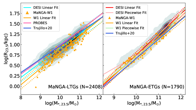
Figure 13: Size–stellar mass relation for LTGs (left-hand panel) and ETGs (right-hand panel). In each panel, grey filled contours represent the distribution of our DESI photometric data; the cyan (LTGs) and red (ETGs) lines are the orthogonal best fit for the corresponding populations. The orange triangles and solid line represent the same structural parameters measured with the WISE (W1) data. The dotted lines in each panel correspond to the 1$\sigma$ scatter about the best-fitting line. In the left-hand panel, the $R-M_{*}$ relation for ${\sim}$1100 PROBES galaxies is presented as a pink line (Stone et al., 2021). Both panels show the $R-M_{*}$ relation of Trujillo et al. (2020) based on ${\sim}$1000 galaxies. Piece-wise linear fits to the DESI and WISE data are also shown for the ETGs (see the text for details.)

Figure 13 shows the $R-M_{*}$ relation for LTG and ETG populations measured from our DESI and WISE photometry. The parameter distributions are shown as density contours, while the cyan (red) lines represent the orthogonal best fits to the LTG (ETG) data. The pink solid line shows the best-fitting relation from Stone et al. (2021) who used a compilation of LTG surveys with DESI imaging for $\sim$1100 spiral galaxies. The photometric analyses for our MaNGA and PROBES samples use the same methods (DESI photometry, AUTOPROF , surface brightness profile treatments, photometric band). It is therefore not surprising that our linear regression should match the PROBES fit so well. Stone et al. (2021) also report a scatter of $0.099^{+0.002}_{-0.003}$ which is in perfect agreement with the observed scatter of our MaNGA galaxies. Overall, the MaNGA and PROBES LTGs have matching $R-M_{*}$ properties measured from a distinct sample of galaxies (though matching analysis routines).

The left-hand panel of Figure 13 (blue solid line) also presents a comparison with the linear $R-M_{*}$ relation from Trujillo et al. (2020) who reported a slope of $0.318\pm 0.014$ and a scatter of $0.087\pm 0.005$, based on SDSS-i band imaging and using isophotal sizes at 23.5 mag arcsec^-2 . The different photometric band used in our respective analysis may explain the slight slope and scatter mismatch for our respective $R-M_{*}$ relations.

For LTGs, the slope of the $R-M_{*}$ relation is independent of wavelength (Table 5). This agrees with Lange et al. (2015) who showed minimal variations in the slope of the $R-M_{*}$ relation for 8400 GAMA galaxies (Driver et al., 2009) across the ugrizZYJHK photometric bands modulo random variations (see Table 6). The actual value of our respective slopes differ on account of our respective size metric choices (effective vs. isophotal radius).

The density map and the red solid line in the right-hand panel of Figure 13 represent the $R-M_{*}$ relation for our ETG sample. The single linear $R-M_{*}$ relation for ETGs is steeper (larger slope) and tighter (smaller scatter) than for LTGs. The slope and scatter of the ETGs $R-M_{*}$ relation is likely controlled by their formation via repeated mergers on high impact parameter orbits (Shen et al., 2003). Dry (gas-less) mergers are the most plausible explanation for the steep size growth of the ETGs From $z\sim 1$ to now (Huertas-Company et al., 2013).

Our linear $R-M_{*}$ relation is in general agreement with (Trujillo et al., 2020), who found a slope of $0.453\pm 0.011$ and an observed scatter of $0.042\pm 0.004$ for 280 galaxies. The differences in best-fitting parameters are a result of the choice photometric band (SDSS-i) and least-square linear regression. Lange et al. (2015) found a range of $R-M_{*}$ relation slopes of $0.46-0.56$ (scatter not reported) for GAMA galaxies (Driver et al., 2009) in the SDSS-z band. They also used effective radii as the size metric making comparisons challenging. The exact value of the slope in Lange et al. (2015) depends largely on their morphological assignments of ETGs as guided by Seŕsic index, dust-corrected optical colour, and visual classification. We find a general trend that the $R-M_{*}$ relation for ETGs is steeper (shallower) if effective (isophotal) radii are used.

Figure 13 also presents the linear $R-M_{*}$ relation for our WISE W1 photometry with the orange line and triangles for the LTGs/ETGs in the left-/right-hand panels. This relation (slope and scatter) is essentially the same as that inferred from DESI $z$-band images for our LTGs, further highlighting our conclusions in Table 5 that the slope and scatter for LTG $R-M_{*}$ relation is independent of the wavelength. The scatter and slope of the ETG WISE $R-M_{*}$ relation differ slightly from their $z$-band counterpart. This result is similar to that of Lange et al. (2015), who found large random variations in the slope of $R-M_{*}$ relation for ETGs.

Along with the projected $R-M_{*}$ relation (Table 5), we can calculate this relation with physical radii (see Section 2.2.1). Table 5 presents the physical $r_{23.5}-M_{*}$ relation for the DESI z and W1 photometric bands. The projected and physical $r-M_{*}$ relations for LTGs are equal by definition. For ETGs physical sizes increase by 4/3 relative to projected values (Hernquist, 1990; Chiosi & Carraro, 2002), resulting in a predictable change in zero-points (by 0.125 dex) of the best-fitting relation. The best linear fits to physical relations are presented in Table 5.

Band	N	M∗ limit	Piece-wise fits
(1)	(2)	(3)	(4)
DESI-z	1854	$\rm\log M_{*}\leq 10.20$	$\rm 0.31(\log M_{*}-10.20)+0.80$
		$\rm\log M_{*}>10.20$	$\rm 0.55(\log M_{*}-10.20)+0.80$
W1	97	$\rm\log M_{*}\leq 10.81$	$\rm 0.41(\log M_{*}-10.81)+1.05$
		$\rm\log M_{*}>10.81$	$\rm 0.52(\log M_{*}-10.81)+1.05$

Table 7: Linear piece-wise $R-M_{*}$ relations for MaNGA-ETGs. columns (1) and (2) give the photometric band and number of data points used for the fit; column (3) shows the stellar mass limit for the change in slope; and column (4) presents the piece-wise fits.

Given the bimodalities in stellar mass and sizes for ETGs seen in Figure 3, we also model the $R-M_{*}$ relation based on DESI and WISE imaging with a double piece-wise linear fit (see Table 7). It is found that the slopes of our $R-M_{*}$ relations for LTGs and ETGs based on DESI and WISE data agree closely with the theoretical expectations. For LTGs, it can be shown that $R_{opt}\propto M_{*}^{0.33}$ for virialized galaxy discs and assuming constant $\Upsilon_{*}$ per galaxy (Courteau et al., 2007). Various scaling arguments connecting structure formation to primordial density fluctuations (Blumenthal et al., 1984) also suggest that massive ETGs ($\log(M_{*}/M_{\odot})\geq 10$) have $R\propto M_{*}^{0.53}$ (Burstein et al., 1997; Chiosi & Carraro, 2002; D’Onofrio et al., 2020). The slope for lower mass ETGs is predicted to be shallower with $R\propto M_{*}^{0.33}$; closer to that of LTGs in the same mass range (Chiosi & Carraro, 2002; Woo et al., 2008). The piece-wise linear fit slopes for ETGs (Table 7), with a low and high mass transition at $\log(M_{*}/M_{\odot})\sim 10.2$ matches theoretical expectations (0.33/0.53) in the same stellar mass bins quite closely (Blumenthal et al., 1984; Chiosi & Carraro, 2002). The same statement holds for the WISE data with stellar mass transition being larger than the optical data. However, this larger stellar mass transition could be attributed to small statistics for low-mass WISE ETGs.

The agreement between the observed and predicted $R-M_{*}$ slopes is certainly encouraging. However, a complete data-model investigation should also match the zero-points, and scatters of observed scaling relations. Our MaNGA data base serves as a stepping stone for such a comparison with theoretical and numerical models of galaxy formation and structure.

In the next section, we explore other size metrics and their effects on slopes and scatters of the $R-M_{*}$ relation.

6.2 Slope and scatter variations of the $R-M_{*}$ relation

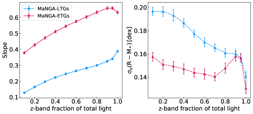
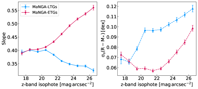
Figure 14: Variations of the slope and orthogonal scatter of the $R-M_{*}$ relation of LTGs (blue) and ETGs (red) for different size measurements. The top panels show size measurements at various fractions of total light. Isophotal size measurements are presented in the bottom panels. $R-M_{*}$ slopes are presented in the left-hand panels with connected squares. Observed orthogonal scatter measurements are presented in the right-hand panels with connected triangles. The error bars on all points correspond to bootstrap uncertainties.

The spatially-resolved nature of our photometric solutions enables a detailed study of the $R-M_{*}$ relation with a suite of size metrics for both LTGs and ETGs, as shown in Figure 14.

6.2.1 Slope variations of the $R-M_{*}$ relation

The left-hand panels of Figure 14 show variations of the slope of the $R-M_{*}$ relation with size metrics measured relative to the total light (top panels) and isophotal levels (bottom panels). For both morphologies, the slope of the $R-M_{*}$ relation increases linearly with light fraction. However, the $R-M_{*}$ slopes for LTGs and ETGs with sizes measured at different isophotal levels have nearly opposite behaviours, as seen in the bottom left-hand panel of Figure 14. The $R-M_{*}$ relation slope for LTGs settles to the theoretical value of 0.33 (Courteau et al., 2007) between 23 and 26 $z$-mag arcsec^-2 . The slope for the ETGs grows steadily before flattening to a value of $\sim$0.53 at or beyond 26 $z$-mag arcsec^-2 . The value where the slope flatten agrees with the theoretical prediction found in Burstein et al. (1997) and Chiosi & Carraro (2002). The exact nature of the slope of the $R-M_{*}$ relation as a function of size metric can be related to the interplay between the relative slopes of the surface brightness profiles and COG.

For LTGs, $R-M_{*}$ slopes range from 0.13 to 0.39 (fractional) or 0.39 to 0.33 (isophotal); the slopes are always smaller if measured relative to the total light, and the trends are opposite. For ETGs, $R-M_{*}$ slopes range from 0.42 to 0.62 (fractional) or 0.39 to 0.63 (isophotal). The steeper $R-M_{*}$ slope for ETGs (see Section 6.1) is expected from a high occurrence of dry mergers and feedback from stars and supermassive black holes (Shen et al., 2003; Huertas-Company et al., 2013). The use of $R_{\rm eff}$ also yields a closer match to theoretical predictions of the $R-M_{*}$ slope. The theoretical prediction can also be matched with isophotal radii by binning galaxies in stellar mass (similar to Chiosi et al., 2020).

6.2.2 Scatter variations of the $R-M_{*}$ relation

The right-hand panels of Figure 14 show variations in the orthogonal scatter of the $R-M_{*}$ relation with size metrics measured relative to the total light (top panels) and isophotal levels (bottom panels). For both morphologies, the $R-M_{*}$ scatter profiles (top right-hand panel of Figure 14) show different behaviours. The scatter for LTGs decreases monotonically from 0.20 to 0.15 dex with increasing total light fraction. The tightest $R-M_{*}$ relation is found when all the light from our photometry is taken into account. For ETGs, the scatter of the $R-M_{*}$ relation is mostly constant around $\sim$0.14 dex for all size metrics.

Trends with isophotal sizes differ: smallest orthogonal scatter for the $R-M_{*}$ relation is found at 18.5 (21.6) $z$-mag arcsec^-2 for LTG (ETG) populations. Our conclusions remain the same if forward scatter was used instead of orthogonal. This result comes as a surprise in light of the current literature that points to the isophotal radius of 23.5 mag arcsec^-2 that minimizes the scatter of VRL scaling relations (Courteau, 1996; Hall et al., 2012). More recently, Trujillo et al. (2020) found the radius corresponding to a stellar surface density of $\rm 1\,M_{\odot}\,pc^{-2}$ also shows a tight $R-M_{*}$ relation along with the added benefit of definition motivated by the physics of star formation in galaxies. This radius corresponds to a fainter isophote ($\sim$26 mag arcsec^-2 ) which is larger than the isophotal radius of 23.5 mag arcsec^-2 . Our findings contradict this as the radius giving the tightest $R-M_{*}$ relation is found to be at 18.5 (21.5) z mag arcsec^-2 for LTGs (ETGs). Sánchez Almeida (2020) performed a similar exercise and found the isophotal radius of $\rm 24.7\pm 0.5$ $r$-mag arcsec^-2 minimizes the scatter. The difference between our results are related to the definition of scatter of a linear relation (half of inter-quartile range vs. rms) and the choice of the photometric band (DESI-z vs. SDSS-r).

Scatter values are also always smaller for isophotal sizes than light fraction sizes. This occurs because light fraction sizes encompass multiple surface brightness levels, thus enhancing the mix of stellar populations at any radius and yielding larger $R-M_{*}$ scatter values (see e.g. Trujillo et al., 2020). The results in this section are further corroborated with our MIR photometry that show similar trends [minimum scatter on 17.5(20) mag arcsec^-2 for ETGs(LTGs)]. These are not shown in Figure 14 for simplicity. It has been noted the the isophotal level of 23.5 $i$-mag arcsec^-2 minimizes scatter of the TFR (Giovanelli et al., 1994; Hall et al., 2012). In an upcoming publication, we investigate the radius, if any, that minimizes the scatter of the VRL scaling relations simultaneously.

6.3 $\Sigma_{1}$-stellar mass ($\Sigma_{1}$–M_∗) relation

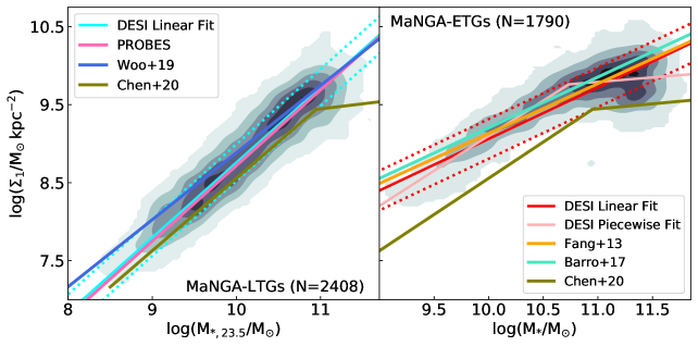
Figure 15: $\Sigma_{1}$ - stellar mass relation for the LTGs (left-hand panel) and ETGs (right-hand panel) using our optical DESI photometry. The density maps in grey show the data distribution. Orthogonal best fits are represented by solid cyan (LTGs) and red (ETGs) lines; the dotted lines show 1 $\sigma$ scatter for the best-fitting relations. For LTGs, the stellar masses are measured as the average of five MLCRs presented in Section 2.2.4. For ETGs, the stellar masses are measured using the MLCR of B19. We compare our LTG relation with Woo & Ellison (2019) and Stone et al. (2021), and our ETG relation with Fang et al. (2013) and Barro et al. (2017) (see the text for the redshift range). Both panels show the $\Sigma_{1}-M_{*}$ relation of Chen et al. (2020a) which fits all morphological types. A piece-wise linear fit to the DESI data is also shown for the ETGs (see the text for details).

The $\Sigma_{1}-M_{*}$ relation reveals information about the star formation and merger histories of galaxies (Barro et al., 2017) and the physical/time evolution of their central components of galaxies (Woo & Ellison, 2019; Chen et al., 2020a; Chen et al., 2020b). While the calculation of the stellar surface density at 1 kpc can be challenging given large distance errors and saturation issues, $\Sigma_{1}$ traces properties as the bulge component with the added advantage of being model-independent. Figure 15 shows the $\Sigma_{1}-M_{*}$ relation for MaNGA LTGs and ETGs based on our DESI optical photometry. Because the WISE data cannot resolve 1-kpc regions for MaNGA galaxies, this section on $\Sigma_{1}$ only uses our optical photometry.

Our orthogonal fit parameters for the $\Sigma_{1}-M_{*}$ relation are presented in the bottom row of Table 5. Stone et al. (2021) found a similar $\Sigma_{1}-M_{*}$ relation with a slope of $1.005^{0.021}_{0.035}$ and a scatter of $0.23\pm 0.01$ dex for their PROBES sample.

This relation is also fit by Woo & Ellison (2019) who found a $\Sigma_{1}-M_{*}$ slope of 0.86 and a scatter of 0.24 dex using ${\sim}2100$ MaNGA galaxies with SDSS photometry and MPA-JHU stellar masses (Brinchmann et al., 2004; Kauffmann et al., 2004). Their different slope may be explained by their use of the SDSS i band, a different definition of stellar mass and a least-square linear fit. Their fit is not a good match to our relation (Figure 15).

Our $\Sigma_{1}-M_{*}$ slope for ETGs matches closely to that of Fang et al. (2013) whose study of ${\sim}1300$ quenched galaxies selected from the SDSS with $z<0.075$ yielded a slope of $0.64^{+0.23}_{-0.20}$. However, their reported scatter of 0.16 dex is significantly smaller than ours. This disagreement could be due to sample selection, choice of MLCRs to calculate stellar masses and the assumptions about the IMF. The conversion of light into stellar mass is also inherently uncertain. While our study targets morphologically selected ETGs, Fang et al. (2013) selected green valley galaxies that are quenched. Even though there is overlap in these samples, an ETG sample and green valley/quenched sample are different. For instance, green valley galaxies can exhibit a range of morphologies (Mendez et al., 2011) and ETGs can show large range in star formation histories. In principle, $\Sigma_{1}$ should be more sensitive to the star formation history than visual morphologies explaining our larger scatter for the relation.

The right-hand panel of Figure 15 also shows the $\Sigma_{1}-M_{*}$ relation of Barro et al. (2017) for CANDELS GOODS-S galaxies at $0.5<z<1.0$ (Guo et al., 2013) who reported a slope of $0.65\pm 0.03$ and a zero-point of $2.71\pm 0.05$. For quiescent galaxies, Barro et al. (2017) found that the slope of the $\Sigma_{1}-M_{*}$ relation remains constant as a function of redshift; only the zero-point evolves with time. For a fixed stellar mass bin, $\Sigma_{1}$ should decrease over time (Barro et al., 2017). Our similar slopes and smaller zero-point strengthen this assertion as our local universe MaNGA ETGs ($z<0.15$) achieve the same slope and a smaller zero point.

An interesting feature of the $\Sigma_{1}-M_{*}$ relation for ETGs is its flattening for $\log(M_{*}/M_{\odot})\geq 10.7$. As a result of this feature, and as stated for the $R-M_{*}$ relation of ETGs Section 6.1, caution should be taken while fitting a linear relation to the ETG $\Sigma_{1}-M_{*}$ relation (see the right-hand panel of Figure 15). Along with the linear regression, we fit piece-wise linear function to the data distribution, with $\log\Sigma_{1}=0.90(\log M_{*}-10.73)+9.76$ for $\log M_{*}\leq 10.73$, and $\log\Sigma_{1}=0.12(\log M_{*}-10.73)+9.76$ for $\log M_{*}>10.73$. We note that the transition in stellar mass at $\log M_{*}\sim 10.7$ in this piece-wise fit is mirrored in the bimodal distribution of stellar masses for ETGs seen in Figure 3. However, the stellar mass transition in the $R-M_{*}$ relation of ETGs is found at $\rm\log M_{*}\sim 10.2$. We are reminded that the bivariate distributions are controlled by two random variables.

Chen et al. (2020a) also used a piece-wise function to describe the $\Sigma_{1}-M_{*}$ relation for the complete MaNGA sample calculated to be: $\log\Sigma_{1}=0.93(\log M_{*}-10.95)+9.44$ for $\log M_{*}\leq 10.95$, and $\log\Sigma_{1}=0.13(\log M_{*}-10.95)+9.44$ for $\log M_{*}>10.95$. Their piece-wise linear fit is shown in the left- and right-hand panels of Figure 15. Their slopes for the low- and high-mass ends of the fit match ours quite well. However, the disagreement in our respective zero-points is significant and may result from our respective stellar mass calculations and different samples. Chen et al. (2020a) used stellar masses provided by the NSA (Blanton et al., 2011); our procedure is described in Section 2.2.4. Indeed, a large difference is found between the stellar masses by NSA and in this study; our photometry results in larger stellar masses by 0.34 (0.40) dex for LTGs (ETGs) that could be due to the systematic offsets of the MLCRs (see Figure 10). Chen et al. (2020a) fit a linear piece-wise function to the full MaNGA sample while our fit is restricted to ETGs. Both of these effects could cause the observed zero point difference, although it is surprising that the slopes remain unaffected.

For LTGs and low-mass ETGs, the slope of the $\Sigma_{1}-M_{*}$ relation near unity (0.96 and 0.90) is suggestive of a co-evolution of the inner and outer regions through star formation and environmental interactions. Indeed, these galaxies may have an enhanced $sSFR(=SFR/M_{*})$ which builds up stellar mass in their inner regions (Woo & Ellison, 2019). The shallower $\Sigma_{1}-M_{*}$ slope (0.13) at the high-mass end for ETGs likely applies to galaxies with little star formation but ongoing overall accretion, leading to a flattening of the $\Sigma_{1}-M_{*}$ relation at $\Sigma_{1}\sim 10^{10}\rm\,M_{\odot}kpc^{-2}$. A complimentary explanation for the saturation of $\Sigma_{1}$ in high mass ETGs involves partially depleted central cores due to coalescing black holes at high redshifts (King & Minkowski, 1966; Ferrarese et al., 1994; Lauer et al., 1995; Gebhardt et al., 1996; Graham & Guzmán, 2003). A proper appreciation of the saturation of $\Sigma_{1}$ in galaxies will require additional data, such as SFRs, maps of neutral and molecular gas reservoirs, environmental parameters to characterize interactions and gas infall, and more. While some of these data still exist, a detailed investigations of the shallower slope at the high-mass end is beyond the scope of this study. We also caution that $\Sigma_{1}$ may be sensitive to projection, dust extinction, and stellar population effects.

7 Summary and Future Work

We have presented high-quality optical and MIR surface brightness profiles and environmental properties for the MaNGA galaxy survey. We made use of DESI imaging and our software (AUTOPROF ; (Stone et al., 2021)) to extract azimuthally averaged optical surface brightness profiles. On average, the DESI photometry reaches ${\sim}2$ mag arcsec^-2 deeper than the SDSS photometry in the gr photometric bands which arises from a combination of deeper DESI imaging and our novel technique, AUTOPROF . The WISE profiles are extracted from the WXSC (Jarrett et al., 2019) which uses deconvolution techniques to achieve a higher resolution than the native WISE imaging. 70 per cent (33 per cent) of the WISE W1 (W2) surface brightness profiles are as deep in radial extent as the DESI photometry and can be used to compute scaling relations at the fiducial isophotal radius $R_{23.5,z}$.

Excellent agreement is found between most model-independent structural parameters from AUTOPROF and those obtained with well-tested surface photometry routines based on the XVISTA software package for astronomical image processing (Courteau, 1996). Disagreements between AUTOPROF , XVISTA and the literature, are largely found for parameters that scale with total light such as effective radii, effective surface brightness, and concentration indices. The bimodal nature in the distribution of some structural parameters is also suggestive of distinct galaxy populations in the Universe.

Detailed comparisons of our surface brightness profiles and structural parameters with other studies were presented. The non-parametric surface brightness profiles from AUTOPROF (DESI) and GC18 (SDSS) agree well, even reproducing small local variations. However, the reconstructed surface brightness profiles from the bulge-to-disc decompositions of GC18 and F19 exhibit large differences (${\sim 0.4}$ mag arcsec^-2 ) demonstrating the challenges involved in such parametric modelling. Moreover, similar disagreements are found between our model-independent surface brightness profiles and the parametric decompositions of both GC18 and F19, highlighting once again the fragile nature of parametric modelling.

Our comparisons of effective radii and apparent magnitudes with PYMORPH of F19 have also revealed disagreements for $R_{\rm eff}$, especially for ETGs $(rms\sim 0.2\,$)dex. Better comparisons are found for isophotal radii $(rms\sim 0.05\,$)dex, demonstrating the superior reproducibility of isophotal sizes over those measured relative to total light fractions. Our apparent magnitudes are also typically brighter than those of F19 by $\sim$0.1 dex. This is expected as, unlike parametric models, our non-parametric surface brightness extraction captures all the light. The GALFIT implementations of GC18 and F19 preferentially favor high S/N regions and systematically predict fainter magnitudes for low S/N. These systematic effects average out to fainter total integrated light, relative to our non-parametric results.

Our stellar mass estimates, measured at $\rm M_{*}(R_{23.5}^{z})$ and obtained from multiband photometry and various MLCRs, compare favorably with those found in the literature, such as MPA-JHU catalogue (Kauffmann et al., 2003), NSA photometry (Blanton & Roweis, 2007), Pipe3D (Sánchez et al., 2016), and P19. Our stellar masses for LTGs, based on the average of multiple MLCRs from RC15, Z17, and B19, are 0.24 dex smaller than those of P19. This offset is explained by the modelling of SFHs by P19 that systematically biases $\Upsilon_{*}$ high. Our stellar masses for ETGs, based on the MLCR from B19, are 0.11 dex smaller than those of P19. The largest stellar mass differences, found for the NSA stellar mass estimates with an rms of 0.34 (0.40) dex for LTGs (ETGs), may stem from uncertainties in the NSA elliptical-Petrosian photometry. The best match with our stellar mass estimates is found for the MPA-JHU catalogue, with an rms of 0.21 (0.11) dex for LTGs (ETGs).

We also present WISE photometry for a subset of $\sim 300$ MaNGA galaxies. It provides an independent measure of stellar masses, which agree with our optical estimates within 0.21 dex (see also Taylor et al., 2011). Dust extinction may explain the small systematic differences in the stellar mass estimates of LTGs. In addition to providing accurate stellar masses, spatially-resolved MIR fluxes are most valuable for studies of the star formation main-sequence, SFR$-M_{*}$ (Cluver et al., 2017; Hall et al., 2018) stellar population properties (Cluver et al., 2014, 2020).

The slope and scatter of the $R-L_{*}$ and $R-M_{*}$ relations for LTGs are found to be independent of bandpass (from g to W2 Table 5). For ETGs, slope variations for the $R-M_{*}$ relation from bluer to redder bands can be linked to varying stellar populations over a range of stellar masses (Lange et al., 2015). The $R-L_{*}$ and $R-M_{*}$ slopes and scatters for LTGs and ETGs also agree well, within 1 $\sigma$, with published values (see Figures 13 and 15).

We have examined the variations of the slope and scatter of the $R-M_{*}$ relation for a range of size metrics. The slopes of the $R-M_{*}$ relations for LTGs and ETGs with size metrics measured relative to total light grow linearly with fraction of total light. Conversely, slopes calculated using isophotal sizes decrease (increase) for LTGs (ETGs) from brighter to fainter regions. These trends are dictated by the relative slope variations in the surface brightness profiles and curves of growth.

Isophotal sizes also yield tighter $R-M_{*}$ relations (smaller scatter) than sizes measured at relative fractions of total light. The isophotal radius measured at 18.5 (21.5) mag arcsec^-2 also yields the tightest $R-M_{*}$ relation for the LTG (ETG) population by orthogonal scatter. Our orthogonal linear fits result in slopes for the LTGs abs ETGs that match theoretical predictions of the $R-M_{*}$ relations.

The $\Sigma_{1}-M_{*}$ relation is also presented for both MaNGA LTGs and ETGs and an excellent agreement is found with the literature. For LTGs, the slope of the $\Sigma_{1}-M_{*}$ relation is near unity, indicating a co-evolution of stellar mass and $\Sigma_{1}$ that is driven by enhanced star formation and environmental effects. For ETGs, a near constant $\Sigma_{1}$ is found for $M_{*}>10.5$. A piecewise linear function was adopted to better match the $\Sigma_{1}-M_{*}$ distribution. The saturation of $\Sigma_{1}$ at high stellar mass could be related to SFRs, environment, neutral/molecular gas distribution, etc.

The multiband photometry, environmental parameters, and structural scaling relations presented in our study may be used to constrain stellar populations models, test semi-analytic or numerical models of galaxy formation, and test their subgrid physics prescriptions (Dutton & van den Bosch, 2009; Brook et al., 2012; Henriques et al., 2015). While extensive, the photometry and scaling relations studied here only inform us about baryonic properties of galaxies. An essential aspect of galaxy formation and evolution is understanding the co-evolution of baryons and dark matter through a simultaneous study of photometric and kinematic properties of galaxies (Courteau et al., 2007; Hall et al., 2012; Ouellette et al., 2017). The MaNGA survey includes dynamical information for all observed galaxies, making this an exciting avenue for related investigations.

Data Availability

All data are incorporated into this paper and its online supplementary material.

Appendix A Surface Brightness Profiles

This Appendix shows the output format of the DESI-grz and WISE W1, W2 surface brightness profiles that are provided as supplementary material. The DESI and WISE surface brightness profiles are provided in the AB and Vega magnitude systems, respectively. The conversions from Vega to AB magnitudes in the W1 and W2 bands are given by (Jarrett et al., 2013):

$$\rm m_{AB}^{{\it W1}}=m_{Vega}^{{\it W1}}+2.683,$$ (6)

$$\rm m_{AB}^{W2}=m_{Vega}^{W2}+3.319.$$ (7)

Column	Unit	Description
(1)	(2)	(3)
R	arcsec	Semimajor axis length of the isophote
SB	mag arcsec-2	Median surface brightness in the AB magnitude system
SB_E	mag arcsec-2	Error on the surface brightness
MAG	mag	Total magnitude within the isophote, computed by integrating the surface brightness profile
MAG_E	mag	Error on the total magnitude within the isophote
ELLIP	–	Ellipticity of the isophote; $\epsilon=1-b/a$, where $b$ is the semi-minor axis length of the isophote, and $a=R$.
ELLIP_E	–	Error on the ellipticity, computed by analysing the local variability within 1 PSF
PA	∘	Position angle of isophote measured from north to east
PA_E	∘	Error on the position angle, computed by analysing the local variability within 1 PSF
MAG_DIRECT	mag	Total magnitude within the isophote computed by flux summation
SB_FIX	mag arcsec-2	Average surface brightness in the AB magnitude system along isophote with ellipticity and position angle set to global values
SB_FIX_E	mag arcsec-2	Error on SB_FIX
MAG_FIX	mag	Total magnitude enclosed within the isophote. Computed by integrating SB_FIX profile
MAG_FIX_E	mag	Error on MAG_FIX

Table 8: Output format of the DESI grz surface brightness profiles provided as supplementary material. Column (1) refers to the column names in each galaxy surface brightness profile; Column (2) shows the units for each parameter; Column (3) describes each profile entry. All DESI-grz surface brightness profiles are named with the MaNGA-ID followed with the extension "_AP.prof"

Column	Unit	Description
(1)	(2)	(3)
radius	arcsec	Semimajor axis length of the isophote
SBpix	–	Surface brightness in digital number along the isophote
SBmag	${{{{\rm mag}~{}{\rm arcsec}}^{-2}}}$	Surface brightness in mag arcsec-2 along the isophote in the Vega magnitude system
SBerr	${{{{\rm mag}~{}{\rm arcsec}}^{-2}}}$	Error on surface brightness in the Vega magnitude system
SBtotmod	${{{{\rm mag}~{}{\rm arcsec}}^{-2}}}$	Total surface brightness for the bulge+disc model in the Vega magnitude system (Jarrett et al., 2019)
SBbulge	${{{{\rm mag}~{}{\rm arcsec}}^{-2}}}$	Surface brightness of the bulge component in the Vega magnitude system (Jarrett et al., 2019)
SBdisk	${{{{\rm mag}~{}{\rm arcsec}}^{-2}}}$	Surface brightness of the disc component in the Vega magnitude system (Jarrett et al., 2019)

Table 9: Output format of the WISE W1, W2 surface brightness profiles provided as supplementary material. Column (1) refers to the column names in each galaxy surface brightness profile; Column (2) shows the units for the parameter; Column (3) describes each profile entry. All WISE W1, W2 surface brightness profiles are named with the WISE catalogue name followed with the extension ".profile.w1/w2.txt". A separate file named "DESI-WISE-index.tbl" provides a conversion table between the MaNGA-ID and WISE-NAME.

References

- Abazajian et al. (2009) Abazajian K. N., et al., 2009, ApJS, 182, 543
- Allen et al. (2015) Allen J. T., et al., 2015, MNRAS, 446, 1567
- Argudo-Fernández et al. (2015) Argudo-Fernández M., et al., 2015, A&A, 578, A110
- Arora et al. (2019) Arora N., Fossati M., Fontanot F., Hirschmann M., Wilman D. J., 2019, MNRAS, 489, 1606
- Astropy Collaboration et al. (2013) Astropy Collaboration et al., 2013, A&A, 558, A33
- Bacon et al. (2001) Bacon R., et al., 2001, MNRAS, 326, 23
- Barro et al. (2017) Barro G., et al., 2017, ApJ, 840, 47
- Blanton & Roweis (2007) Blanton M. R., Roweis S., 2007, AJ, 133, 734
- Blanton et al. (2011) Blanton M. R., Kazin E., Muna D., Weaver B. A., Price-Whelan A., 2011, AJ, 142, 31
- Bluck et al. (2020) Bluck A. F. L., et al., 2020, MNRAS, 499, 230
- Blumenthal et al. (1984) Blumenthal G. R., Faber S. M., Primack J. R., Rees M. J., 1984, Nature, 311, 517
- Brinchmann et al. (2004) Brinchmann J., Charlot S., White S. D. M., Tremonti C., Kauffmann G., Heckman T., Brinkmann J., 2004, MNRAS, 351, 1151
- Brook et al. (2012) Brook C. B., Stinson G., Gibson B. K., Wadsley J., Quinn T., 2012, MNRAS, 424, 1275
- Bruzual & Charlot (2003) Bruzual G., Charlot S., 2003, MNRAS, 344, 1000
- Bundy et al. (2015) Bundy K., et al., 2015, ApJ, 798, 7
- Burstein et al. (1997) Burstein D., Bender R., Faber S., Nolthenius R., 1997, AJ, 114, 1365
- Cano-Díaz et al. (2016) Cano-Díaz M., et al., 2016, ApJ, 821, L26
- Cappellari et al. (2011) Cappellari M., et al., 2011, MNRAS, 416, 1680
- Chen et al. (2020a) Chen G., Zhang H.-X., Kong X., Lin Z., Liang Z., Chen X., Chen Z., Song Z., 2020a, ApJ, 895, 146
- Chen et al. (2020b) Chen Z., et al., 2020b, ApJ, 897, 102
- Chiosi & Carraro (2002) Chiosi C., Carraro G., 2002, MNRAS, 335, 335
- Chiosi et al. (2020) Chiosi C., D’Onofrio M., Merlin E., Piovan L., Marziani P., 2020, A&A, 643, A136
- Ciotti (1991) Ciotti L., 1991, A&A, 249, 99
- Cluver et al. (2014) Cluver M. E., et al., 2014, ApJ, 782, 90
- Cluver et al. (2017) Cluver M. E., Jarrett T. H., Dale D. A., Smith J. D. T., August T., Brown M. J. I., 2017, ApJ, 850, 68
- Cluver et al. (2020) Cluver M. E., et al., 2020, ApJ, 898, 20
- Conroy & Gunn (2010) Conroy C., Gunn J. E., 2010, ApJ, 712, 833
- Cooley & Tukey (1965) Cooley J. W., Tukey J. W., 1965, Mathematics of computation, 19, 297
- Courteau (1996) Courteau S., 1996, ApJS, 103, 363
- Courteau et al. (2007) Courteau S., Dutton A. A., van den Bosch F. C., MacArthur L. A., Dekel A., McIntosh D. H., Dale D. A., 2007, ApJ, 671, 203
- Courteau et al. (2014) Courteau S., et al., 2014, Reviews of Modern Physics, 86, 47
- DESI Collaboration et al. (2016) DESI Collaboration et al., 2016, arXiv e-prints, p. arXiv:1611.00036
- D’Onofrio et al. (2020) D’Onofrio M., Chiosi C., Sciarratta M., Marziani P., 2020, A&A, 641, A94
- Devour & Bell (2019) Devour B. M., Bell E. F., 2019, ApJS, 244, 3
- Dey et al. (2019) Dey A., et al., 2019, AJ, 157, 168
- Domínguez Sánchez et al. (2018) Domínguez Sánchez H., Huertas-Company M., Bernardi M., Tuccillo D., Fischer J. L., 2018, MNRAS, 476, 3661
- Driver et al. (2009) Driver S. P., et al., 2009, Astronomy and Geophysics, 50, 5.12
- Dutton & van den Bosch (2009) Dutton A. A., van den Bosch F. C., 2009, MNRAS, 396, 141
- Dutton et al. (2007) Dutton A. A., van den Bosch F. C., Dekel A., Courteau S., 2007, ApJ, 654, 27
- Erwin (2015) Erwin P., 2015, ApJ, 799, 226
- Etherington & Thomas (2015) Etherington J., Thomas D., 2015, MNRAS, 451, 660
- Fang et al. (2013) Fang J. J., Faber S. M., Koo D. C., Dekel A., 2013, ApJ, 776, 63
- Ferrarese et al. (1994) Ferrarese L., van den Bosch F. C., Ford H. C., Jaffe W., O’Connell R. W., 1994, AJ, 108, 1598
- Fischer et al. (2019) Fischer J.-L., Domínguez Sánchez H., Bernardi M., 2019, MNRAS, 483, 2057
- Fossati et al. (2015) Fossati M., et al., 2015, MNRAS, 446, 2582
- Fossati et al. (2017) Fossati M., et al., 2017, ApJ, 835, 153
- Franx et al. (2008) Franx M., van Dokkum P. G., Förster Schreiber N. M., Wuyts S., Labbé I., Toft S., 2008, ApJ, 688, 770
- García-Benito et al. (2019) García-Benito R., González Delgado R. M., Pérez E., Cid Fernandes R., Sánchez S. F., de Amorim A. L., 2019, A&A, 621, A120
- Gebhardt et al. (1996) Gebhardt K., et al., 1996, AJ, 112, 105
- Gilhuly & Courteau (2018) Gilhuly C., Courteau S., 2018, MNRAS, 477, 845
- Giovanelli et al. (1994) Giovanelli R., Haynes M. P., Salzer J. J., Wegner G., da Costa L. N., Freudling W., 1994, AJ, 107, 2036
- González-Samaniego et al. (2017) González-Samaniego A., Bullock J. S., Boylan-Kolchin M., Fitts A., Elbert O. D., Hopkins P. F., Kereš D., Faucher-Giguère C.-A., 2017, MNRAS, 472, 4786
- Graham & Guzmán (2003) Graham A. W., Guzmán R., 2003, AJ, 125, 2936
- Graham et al. (2001) Graham A. W., Trujillo I., Caon N., 2001, AJ, 122, 1707
- Graham et al. (2018) Graham M. T., et al., 2018, MNRAS, 477, 4711
- Guo et al. (2013) Guo Y., et al., 2013, ApJS, 207, 24
- Hall et al. (2012) Hall M., Courteau S., Dutton A. A., McDonald M., Zhu Y., 2012, MNRAS, 425, 2741
- Hall et al. (2018) Hall C., Courteau S., Jarrett T., Cluver M., Meurer G., Carignan C., Audcent-Ross F., 2018, ApJ, 865, 154
- Henriques et al. (2015) Henriques B. M. B., White S. D. M., Thomas P. A., Angulo R., Guo Q., Lemson G., Springel V., Overzier R., 2015, MNRAS, 451, 2663
- Hernquist (1990) Hernquist L., 1990, ApJ, 356, 359
- Holmberg (1958) Holmberg E., 1958, Meddelanden fran Lunds Astronomiska Observatorium Serie II, 136, 1
- Huertas-Company et al. (2013) Huertas-Company M., et al., 2013, MNRAS, 428, 1715
- Jarrett et al. (2000) Jarrett T. H., Chester T., Cutri R., Schneider S., Skrutskie M., Huchra J. P., 2000, AJ, 119, 2498
- Jarrett et al. (2012) Jarrett T. H., et al., 2012, AJ, 144, 68
- Jarrett et al. (2013) Jarrett T. H., et al., 2013, AJ, 145, 6
- Jarrett et al. (2019) Jarrett T. H., Cluver M. E., Brown M. J. I., Dale D. A., Tsai C. W., Masci F., 2019, ApJS, 245, 25
- Kauffmann et al. (2003) Kauffmann G., et al., 2003, MNRAS, 341, 33
- Kauffmann et al. (2004) Kauffmann G., White S. D. M., Heckman T. M., Ménard B., Brinchmann J., Charlot S., Tremonti C., Brinkmann J., 2004, MNRAS, 353, 713
- King & Minkowski (1966) King I. R., Minkowski R., 1966, ApJ, 143, 1002
- Lange et al. (2015) Lange R., et al., 2015, MNRAS, 447, 2603
- Lauer et al. (1995) Lauer T. R., et al., 1995, AJ, 110, 2622
- Lian et al. (2015) Lian J. H., Li J. R., Yan W., Kong X., 2015, MNRAS, 446, 1449
- MacArthur et al. (2004) MacArthur L. A., Courteau S., Bell E., Holtzman J. A., 2004, ApJS, 152, 175
- Maller et al. (2009) Maller A. H., Berlind A. A., Blanton M. R., Hogg D. W., 2009, ApJ, 691, 394
- Masters et al. (2010) Masters K. L., et al., 2010, MNRAS, 404, 792
- Masters et al. (2019) Masters K. L., et al., 2019, MNRAS, 488, 3396
- McDonald et al. (2009) McDonald M., Courteau S., Tully R. B., 2009, MNRAS, 393, 628
- McDonald et al. (2011) McDonald M., Courteau S., Tully R. B., Roediger J., 2011, MNRAS, 414, 2055
- Méndez-Abreu et al. (2018) Méndez-Abreu J., et al., 2018, MNRAS, 474, 1307
- Mendez et al. (2011) Mendez A. J., Coil A. L., Lotz J., Salim S., Moustakas J., Simard L., 2011, ApJ, 736, 110
- Mo et al. (1998) Mo H. J., Mao S., White S. D. M., 1998, MNRAS, 295, 319
- Molina et al. (2020) Molina M., Ajgaonkar N., Yan R., Ciardullo R., Gronwall C., Eracleous M., Ji X., Blanton M. R., 2020, arXiv e-prints, p. arXiv:2007.08541
- Ouellette et al. (2017) Ouellette N. N. Q., et al., 2017, ApJ, 843, 74
- Pace et al. (2019) Pace Z. J., et al., 2019, ApJ, 883, 83
- Pizagno et al. (2005) Pizagno J., et al., 2005, ApJ, 633, 844
- Renzini (2006) Renzini A., 2006, ARA&A, 44, 141
- Roediger & Courteau (2015) Roediger J. C., Courteau S., 2015, MNRAS, 452, 3209
- Saglia et al. (2010) Saglia R. P., et al., 2010, A&A, 524, A6
- Sánchez Almeida (2020) Sánchez Almeida J., 2020, MNRAS, 495, 78
- Sánchez-Menguiano et al. (2020) Sánchez-Menguiano L., Sánchez Almeida J., Muñoz-Tuñón C., Sánchez S. F., 2020, ApJ, 903, 52
- Sánchez et al. (2016) Sánchez S. F., et al., 2016, Rev. Mex. Astron. Astrofis., 52, 21
- Sánchez et al. (2018) Sánchez S. F., et al., 2018, Rev. Mex. Astron. Astrofis., 54, 217
- Schlegel et al. (1998) Schlegel D. J., Finkbeiner D. P., Davis M., 1998, ApJ, 500, 525
- Shalev-Shwartz & Ben-David (2014) Shalev-Shwartz S., Ben-David S., 2014, Understanding machine learning: From theory to algorithms. Cambridge university press
- Shen et al. (2003) Shen S., Mo H. J., White S. D. M., Blanton M. R., Kauffmann G., Voges W., Brinkmann J., Csabai I., 2003, MNRAS, 343, 978
- Smith et al. (2021) Smith M. J., Arora N., Stone C., Courteau S., Geach J. E., 2021, MNRAS, 503, 96
- Sorce et al. (2013) Sorce J. G., Courtois H. M., Sheth K., Tully R. B., 2013, MNRAS, 433, 751
- Stone & Courteau (2019) Stone C., Courteau S., 2019, ApJ, 882, 6
- Stone et al. (2021) Stone C., Courteau S., Arora N., 2021, ApJ, 912, 41
- Taylor et al. (2011) Taylor E. N., et al., 2011, MNRAS, 418, 1587
- Trujillo et al. (2001) Trujillo I., Graham A. W., Caon N., 2001, MNRAS, 326, 869
- Trujillo et al. (2020) Trujillo I., Chamba N., Knapen J. H., 2020, MNRAS, 493, 87
- Tuccillo et al. (2018) Tuccillo D., Huertas-Company M., Decencière E., Velasco-Forero S., Domínguez Sánchez H., Dimauro P., 2018, MNRAS, 475, 894
- Tully & Verheijen (1997) Tully R. B., Verheijen M. A. W., 1997, ApJ, 484, 145
- Tully et al. (1998) Tully R. B., Pierce M. J., Huang J.-S., Saunders W., Verheijen M. A. W., Witchalls P. L., 1998, AJ, 115, 2264
- Virtanen et al. (2020) Virtanen P., et al., 2020, Nature Methods, 17, 261
- Wake et al. (2017) Wake D. A., et al., 2017, AJ, 154, 86
- Walcher et al. (2014) Walcher C. J., et al., 2014, A&A, 569, A1
- Wilman et al. (2010) Wilman D. J., Zibetti S., Budavári T., 2010, MNRAS, 406, 1701
- Woo & Ellison (2019) Woo J., Ellison S. L., 2019, MNRAS, 487, 1927
- Woo et al. (2008) Woo J., Courteau S., Dekel A., 2008, MNRAS, 390, 1453
- York et al. (2000) York D. G., et al., 2000, AJ, 120, 1579
- Zhang et al. (2017) Zhang H.-X., Puzia T. H., Weisz D. R., 2017, ApJS, 233, 13
- Zheng et al. (2020) Zheng Y., Wild V., Lahén N., Johansson P. H., Law D., Weaver J. R., Jimenez N., 2020, MNRAS, 498, 1259