Non-Gaussianity and the induced gravitational wave background

Abstract

Scalar metric fluctuations generically source a spectrum of gravitational waves at second order in perturbation theory, poising gravitational wave experiments as potentially powerful probes of the small-scale curvature power spectrum. We perform a detailed study of the imprint of primordial non-Gaussianity on these induced gravitational waves, emphasizing the role of both the disconnected and connected components of the primoridal trispectrum. Specializing to local-type non-Gaussianity, we numerically compute all contributions and present results for a variety of enhanced primordial curvature power spectra.

1 Introduction

The paradigm of cosmic inflation [1, 2, 3, 4, 5, 6, 7], together with the $\Lambda$ cold dark matter ($\Lambda$CDM) model, provides a precise description of the Universe on cosmic scales [8, 9, 10, 11]. This model, in which the Universe expands from a hot and dense state following inflation, successfully predicts both the primordial elemental abundances via big bang nucleosynthesis (BBN) [12, 13] as well as the cosmic microwave background radiation (CMB). Furthermore, measurements of the temperature anisotropies of the CMB reveal a red-tilted spectrum of adiabatic and highly Gaussian density fluctuations in excellent agreement with the predictions of standard slow roll inflation [11].

The large ($10-10^{4}$ Mpc) scales measured in the CMB and large-scale structure directly probe (and constrain) the dynamics of inflation around $50-60$ $e$-folds before its end [14]. The later stages of inflation are only weakly constrained by (the nonobservation of) spectral distortions in the CMB [15], as well as the absence of high-energy $\gamma$ rays from ultracompact minihalos [16]. Moreover, the abundances of light elements are insensitive to the state of the Universe prior to BBN and neutrino decoupling (before redshift $z\sim 10^{10}$) [12]. In fact, successful BBN requires only that the Universe was in local thermal equilibrium and expanding in a radiation dominated state by a temperature of around $T\sim 4.1$ MeV [17, 18, 19].

Gravitational waves (GW) offer a unique means to study inhomogeneities on smaller scales and thereby constrain both the later stages of inflation [20] and the evolution of the Universe before BBN [21, 22, 23, 24, 25, 26]. Aside from direct production mechanisms, density perturbations act as a secondary source of stochastic GW backgrounds [27, 28, 29, 30, 31, 32, 33, 34]. Future experiments [35, 36, 37, 38, 39, 40, 41, 42] will probe these “induced” GWs at a variety of frequencies [43, 44, 45, 46, 47, 48, 49, 50, 51, 52, 53, 54, 22, 23, 55, 21, 56, 57, 58, 59, 60, 61, 62, 63, 64, 65, 66, 67, 68, 69, 70, 71, 72, 73, 74], providing valuable information about scales that exit the horizon during inflation long after the modes that eventually seed the CMB anisotropies. These modes reenter the horizon before BBN and subsequently induce gravitational waves at second order in cosmological perturbation theory. Enticingly, the pulsar timing array experiment NANOGrav recently presented evidence for a common process [75] which, though currently lacking Bayesian evidence for the requisite quadrupolar correlations, may well be due to a stochastic GW background [76, 77, 78, 79, 80, 81, 82, 83, 84].

The expected level of GWs induced from a red-tilted spectrum of curvature perturbations extrapolated to small scales, with amplitude $\Delta_{\mathcal{R}}^{2}(k_{\star})\approx 10^{-10}$ at $k_{\star}=0.05\,h$ Mpc^-1 required by the CMB anisotropies, is unobservably tiny [32, 33]. However, there is no a priori reason to expect that such an extrapolation is appropriate over such a large range of scales. In particular, induced GWs are expected to be significant in scenarios where primordial black holes (PBHs) form via the gravitational collapse of small-scale curvature perturbations [85, 86, 87, 88, 89]. GWs therefore provide a powerful probe not only of the initial conditions and expansion history of the Universe but also of the abundance of PBHs and their potential to constitute a sizable fraction of the dark matter [90, 91, 92]. For recent reviews, see Refs. [93, 94, 95, 96].

While the running of the spectral index typically suppresses power on very small scales in canonical models of inflation (see, e.g. [97]), a number of scenarios can enhance the curvature power spectrum on small scales. Examples of modifications to the minimal slow roll scenario include multifield inflation [98, 99], inflaton couplings leading to particle production [100, 101, 102, 47, 103, 51, 104, 105, 106], a plateau in the inflaton potential that causes a period of ultra slow roll [107, 108, 109, 110], and a brief downward step in the potential [111]. In these scenarios the curvature perturbation is often non-Gaussian on these scales, impacting not only PBH formation (which is sensitive to the tail of the probability distribution of density perturbations) but also the induced GW signal.

In this work we revisit the problem of GW backgrounds induced by non-Gaussian curvature perturbations [50, 51, 88, 86, 60, 66, 110, 74]. We focus on local-type non-Gaussianity [88, 86, 60, 66, 110, 74] and show that the induced GW spectrum is in general sensitive to all contributions to the primordial trispectrum. In particular, in addition to the disconnected part of the curvature perturbation’s 4-point correlation function (arising solely via the non-Gaussian modification to the curvature power spectrum itself), the connected component is a nontrivial and important contribution to the induced GW signal, often unaccounted for in the literature.

This paper is organized as follows. In Section 2 we briefly review the calculation of the dimensionless power spectrum $\mathcal{P}_{\lambda}$ of GWs induced by a generic curvature perturbation $\mathcal{R}$, leaving additional details to Appendix A. We proceed to present the complete contribution of the (connected and disconnected parts of the) 4-point correlation function of $\mathcal{R}$ to $\mathcal{P}_{\lambda}$. We then specialize to the case of local non-Gaussianity. Appendix B outlines the derivation in more detail, presenting a diagrammatic interpretation of individual terms. We present results for a variety of primordial curvature power spectra in Section 3 and conclude in Section 4.

2 Gravitational waves induced by scalar perturbations

We work with a perturbed FLRW spacetime in the conformal Newtonian gauge,

$$\mathrm{d}s^{2} =a(\tau)^{2}\left(-\left[1+2\Phi\right]\mathrm{d}\tau^{2}+\left[(1-2\Phi)\delta_{ij}+\frac{1}{2}h_{ij}\right]\mathrm{d}x^{i}\mathrm{d}x^{j}\right),$$ (2.1)

neglecting vector perturbations and first-order tensor perturbations. That is, we consider only tensors sourced at second order in perturbation theory and ignore those at leading order, e.g., a primordial background from inflation. We set $c=\hbar=k_{B}=1$, define the reduced Planck mass $m_{\mathrm{Pl}}=1/\sqrt{8\pi G_{N}}$, and use primes to denote derivatives with respect to conformal time $\tau$. Repeated Latin indices denote a contraction with the Kronecker delta regardless of placement. We assume a fixed equation of state $w=\mkern 1.25mu\overline{\mkern-1.25muP\mkern-1.25mu}\mkern 1.25mu/\mkern 1.25mu\overline{\mkern-1.25mu\rho\mkern-1.25mu}\mkern 1.25mu$, with $\mkern 1.25mu\overline{\mkern-1.25muP\mkern-1.25mu}\mkern 1.25mu$ and $\mkern 1.25mu\overline{\mkern-1.25mu\rho\mkern-1.25mu}\mkern 1.25mu$ the background pressure and energy density, so the scale factor evolves according to

$$a(\tau) =a_{0}\left(\frac{\tau}{\tau_{0}}\right)^{\alpha},$$ (2.2)

where $\alpha=2/(1+3w)$. The conformal-time Hubble parameter is thus

$$\mathcal{H}(\tau)\equiv\frac{a^{\prime}(\tau)}{a(\tau)} =\frac{\alpha}{\tau}.$$ (2.3)

We expand the GWs in Fourier modes as

$$h_{ij}(\tau,\mathbf{x}) =\sum_{\lambda=+,\times}\int\frac{\mathrm{d}^{3}k}{(2\pi)^{3/2}}e^{i\mathbf{k}\cdot\mathbf{x}}\epsilon_{ij}^{\lambda}(\mathbf{k})h_{\lambda}(\tau,\mathbf{k}),$$ (2.4)

where the polarization tensors are

$$\epsilon^{+}_{ij}(\mathbf{k}) =\frac{1}{\sqrt{2}}\left(\epsilon_{i}(\mathbf{k})\epsilon_{j}(\mathbf{k})-\mkern 1.25mu\overline{\mkern-1.25mu\epsilon\mkern-1.25mu}\mkern 1.25mu_{i}(\mathbf{k})\mkern 1.25mu\overline{\mkern-1.25mu\epsilon\mkern-1.25mu}\mkern 1.25mu_{j}(\mathbf{k})\right)$$ (2.5a)

$$\epsilon^{\times}_{ij}(\mathbf{k}) =\frac{1}{\sqrt{2}}\left(\epsilon_{i}(\mathbf{k})\mkern 1.25mu\overline{\mkern-1.25mu\epsilon\mkern-1.25mu}\mkern 1.25mu_{j}(\mathbf{k})+\mkern 1.25mu\overline{\mkern-1.25mu\epsilon\mkern-1.25mu}\mkern 1.25mu_{i}(\mathbf{k})\epsilon_{j}(\mathbf{k})\right)$$ (2.5b)

and $\epsilon_{i}(\mathbf{k})$ and $\mkern 1.25mu\overline{\mkern-1.25mu\epsilon\mkern-1.25mu}\mkern 1.25mu_{i}(\mathbf{k})$ form an orthonormal basis transverse to $\mathbf{k}$. Note that $\epsilon_{ij}^{\lambda}(\mathbf{k})$ are traceless and transverse to $\mathbf{k}$ by construction. The power spectrum of GWs is then defined as

$$\langle h_{\lambda_{1}}(\tau,\mathbf{k}_{1})h_{\lambda_{2}}(\tau,\mathbf{k}_{2})\rangle =\delta^{3}(\mathbf{k}_{1}+\mathbf{k}_{2})\delta^{\lambda_{1}\lambda_{2}}\mathcal{P}_{\lambda_{1}}(\tau,k_{1}).$$ (2.6)

We also define the dimensionless GW power spectrum,

$$\langle h_{\lambda_{1}}(\tau,\mathbf{k}_{1})h_{\lambda_{2}}(\tau,\mathbf{k}_{2})\rangle =\delta^{3}(\mathbf{k}_{1}+\mathbf{k}_{2})\delta^{\lambda_{1}\lambda_{2}}\frac{2\pi^{2}}{k_{1}^{3}}\Delta^{2}_{\lambda_{1}}(\tau,k_{1}).$$ (2.7)

The spatially averaged energy density of gravitational waves on subhorizon scales is

$$\rho_{\mathrm{GW}}(\tau) =\int\mathrm{d}\ln k\,\rho_{\mathrm{GW}}(\tau,k)=\frac{m_{\mathrm{Pl}}^{2}}{16a(\tau)^{2}}\left\langle\mkern 1.25mu\overline{\mkern-1.25mu\partial_{k}h_{ij}\partial_{k}h_{ij}\mkern-1.25mu}\mkern 1.25mu\right\rangle,$$ (2.8)

where the overbar denotes a time average (i.e., over oscillations). The fractional energy density in GWs per logarithmic wavenumber is

$$\Omega_{\mathrm{GW}}(\tau,k)\equiv\frac{\rho_{\mathrm{GW}}(\tau,k)}{\rho_{\mathrm{tot}}(\tau)}=\frac{1}{48}\left(\frac{k}{a(\tau)H(\tau)}\right)^{2}\sum_{\lambda=+,\times}\mkern 1.25mu\overline{\mkern-1.25mu\Delta^{2}_{\lambda}(\tau,k)\mkern-1.25mu}\mkern 1.25mu.$$ (2.9)

The spectrum that would be observed today (assuming emission after reheating) is obtained via the transfer function

$$\Omega_{\mathrm{GW},0}(k)h^{2} =\Omega_{\mathrm{rad},0}h^{2}\left(\frac{g_{\star,0}}{g_{\star,\mathrm{e}}}\right)^{1/3}\Omega_{\mathrm{GW},\mathrm{e}}(k),$$ (2.10)

which for comoving momentum $k$ would be observed at the present-day frequency

$$f=\frac{k/2\pi a_{\mathrm{e}}}{\sqrt{H_{\mathrm{e}}m_{\mathrm{Pl}}}}\left(\Omega_{\mathrm{rad},0}H_{0}^{2}m_{\mathrm{Pl}}^{2}\right)^{1/4}\left(\frac{g_{\star,0}}{g_{\star,\mathrm{e}}}\right)^{1/12}.$$ (2.11)

Here $g_{\star}$ is the number of relativistic degrees of freedom in energy density, $\Omega_{\mathrm{rad},0}$ the present-day abundance of radiation, and $H$ the Hubble parameter; subscripts $\mathrm{e}$ and $0$ denote the time of emission and the present day, respectively. Note that $\Omega_{\mathrm{rad},0}h^{2}\approx 4.2\times 10^{-5}$ with $h=H_{0}/100\,\mathrm{km}\mathrm{s}^{-1}/\mathrm{Mpc}$.

2.1 Induced gravitational wave solution

The induced gravitational waves evolve according to

$$h_{\lambda}^{\prime\prime}(\tau,\mathbf{k})+2\mathcal{H}h_{\lambda}^{\prime}(\tau,\mathbf{k})+k^{2}h_{\lambda}(\tau,\mathbf{k}) =4\mathcal{S}_{\lambda}(\tau,\mathbf{k}),$$ (2.12)

where the source $\mathcal{S}_{\lambda}$ comprises the terms of the (transverse, traceless part of the) Einstein equation that are second order in scalar perturbations. To make contact with primordial physics, it is conventional to express the gravitational potential in terms of the primordial curvature perturbation $\mathcal{R}$ and a transfer function $\Phi(k\tau)$,

$$\Phi(\tau,\mathbf{k}) =\frac{3+3w}{5+3w}\Phi(k\tau)\mathcal{R}(\mathbf{k}).$$ (2.13)

The transfer function $\Phi(k\tau)$ encodes the linear evolution of the Newtonian potential after horizon reentry. In these terms, the source is [32, 33]

$$\mathcal{S}_{\lambda}(\tau,\mathbf{k}) =\int\frac{\mathrm{d}^{3}q}{(2\pi)^{3/2}}Q_{\lambda}(\mathbf{k},\mathbf{q})f(|\mathbf{k}-\mathbf{q}|,q,\tau)\mathcal{R}(\mathbf{q})\mathcal{R}(\mathbf{k}-\mathbf{q}),$$ (2.14)

where $f(|\mathbf{k}-\mathbf{q}|,q,\tau)$ is given by

$$\begin{split}f(p,q,\tau)&=\frac{3(1+w)}{(5+3w)^{2}}\Big{[}2(5+3w)\Phi(p\tau)\Phi(q\tau)+\tau^{2}\left(1+3w\right)^{2}\Phi^{\prime}(p\tau)\Phi^{\prime}(q\tau)\\ &\hphantom{{}={}\frac{3(1+w)}{(5+3w)^{2}}\Big{[}}+2\tau\left(1+3w\right)\left(\Phi(p\tau)\Phi^{\prime}(q\tau)+\Phi^{\prime}(p\tau)\Phi(q\tau)\right)\Big{]}.\end{split}$$ (2.15)

Note that $f(p,q,\tau)$ is symmetric under exchange of $q$ and $p$. The projection factors are

$$Q_{\lambda}(\mathbf{k},\mathbf{q}) \equiv\epsilon_{ij}^{\lambda}(\mathbf{k})q_{i}q_{j}.$$ (2.16)

Taking $\mathbf{k}$ in the $\hat{z}$ direction and writing

$$\mathbf{q} =q\left[\sin\theta\cos\phi,\sin\theta\sin\phi,\cos\theta\right],$$ (2.17)

the projection factors evaluate to

$$Q_{\lambda}(\mathbf{k},\mathbf{q}) =\frac{q^{2}}{\sqrt{2}}\sin^{2}(\theta)\times\begin{cases}\cos(2\phi)&\lambda=+\\ \sin(2\phi)&\lambda=\times.\end{cases}$$ (2.18)

We note that the $\cos(2\phi)$ and $\sin(2\phi)$ terms are absent in some of the intermediate steps in Ref. [33].

The induced GWs are the particular solution of Eq. 2.12,

$$h_{\lambda}(\tau,\mathbf{k})=\frac{4}{a(\tau)}\int^{\tau}_{\tau_{0}}\mathrm{d}\mkern 1.25mu\overline{\mkern-1.25mu\tau\mkern-1.25mu}\mkern 1.25mu\,G_{\mathbf{k}}(\tau,\mkern 1.25mu\overline{\mkern-1.25mu\tau\mkern-1.25mu}\mkern 1.25mu)a(\mkern 1.25mu\overline{\mkern-1.25mu\tau\mkern-1.25mu}\mkern 1.25mu)\mathcal{S}_{\lambda}(\mkern 1.25mu\overline{\mkern-1.25mu\tau\mkern-1.25mu}\mkern 1.25mu,\mathbf{k}),$$ (2.19)

where the Green function $G_{\mathbf{k}}(\tau,\mkern 1.25mu\overline{\mkern-1.25mu\tau\mkern-1.25mu}\mkern 1.25mu)$ obeys the equation of motion

$$\partial_{\tau}^{2}G_{\mathbf{k}}(\tau,\mkern 1.25mu\overline{\mkern-1.25mu\tau\mkern-1.25mu}\mkern 1.25mu)+\left[k^{2}-\frac{a^{\prime\prime}(\tau)}{a(\tau)}\right]G_{\mathbf{k}}(\tau,\mkern 1.25mu\overline{\mkern-1.25mu\tau\mkern-1.25mu}\mkern 1.25mu) =\delta(\tau-\mkern 1.25mu\overline{\mkern-1.25mu\tau\mkern-1.25mu}\mkern 1.25mu).$$ (2.20)

Hence, the power spectrum of the induced GWs is given by

$$\begin{split}\langle h_{\mathbf{k}_{1}}^{\lambda_{1}}h_{\mathbf{k}_{2}}^{\lambda_{2}}\rangle&=16\int\frac{\mathrm{d}^{3}q_{1}}{(2\pi)^{3/2}}\frac{\mathrm{d}^{3}q_{2}}{(2\pi)^{3/2}}\langle\mathcal{R}(\mathbf{q}_{1})\mathcal{R}(\mathbf{k}_{1}-\mathbf{q}_{1})\mathcal{R}(\mathbf{q}_{2})\mathcal{R}(\mathbf{k}_{2}-\mathbf{q}_{2})\rangle Q_{\lambda_{1}}(\mathbf{k}_{1},\mathbf{q}_{1})Q_{\lambda_{2}}(\mathbf{k}_{2},\mathbf{q}_{2})\\ &\hphantom{{}={}16\int\frac{\mathrm{d}^{3}q_{1}}{(2\pi)^{3/2}}\frac{\mathrm{d}^{3}q_{2}}{(2\pi)^{3/2}}}\times I({\left|\mathbf{k}_{1}-\mathbf{q}_{1}\right|},q_{1},\tau_{1})I({\left|\mathbf{k}_{2}-\mathbf{q}_{2}\right|},q_{2},\tau_{2}),\end{split}$$ (2.21)

having defined

$$I(p,q,\tau) =\int_{\tau_{0}}^{\tau}\mathrm{d}\mkern 1.25mu\overline{\mkern-1.25mu\tau\mkern-1.25mu}\mkern 1.25mu\,G_{\mathbf{k}}(\tau,\mkern 1.25mu\overline{\mkern-1.25mu\tau\mkern-1.25mu}\mkern 1.25mu)\frac{a(\mkern 1.25mu\overline{\mkern-1.25mu\tau\mkern-1.25mu}\mkern 1.25mu)}{a(\tau)}f(p,q,\mkern 1.25mu\overline{\mkern-1.25mu\tau\mkern-1.25mu}\mkern 1.25mu).$$ (2.22)

By treating the scalar perturbations to linear order, the time dependence of the induced GW spectrum is decoupled from the primordial curvature power spectrum. For a fixed equation of state, the integrals $I(p,q,\tau)$ can be computed analytically [53].

If we impose statistical homogeneity and isotropy on the curvature perturbation $\mathcal{R}$ and assume $\langle\mathcal{R}\rangle=0$, then its 4-point function splits into disconnected and connected components:

$$\langle\mathcal{R}(\mathbf{k}_{1})\mathcal{R}(\mathbf{k}_{2})\mathcal{R}(\mathbf{k}_{3})\mathcal{R}(\mathbf{k}_{4})\rangle =\langle\mathcal{R}(\mathbf{k}_{1})\mathcal{R}(\mathbf{k}_{2})\mathcal{R}(\mathbf{k}_{3})\mathcal{R}(\mathbf{k}_{4})\rangle_{\mathrm{d}}+\langle\mathcal{R}(\mathbf{k}_{1})\mathcal{R}(\mathbf{k}_{2})\mathcal{R}(\mathbf{k}_{3})\mathcal{R}(\mathbf{k}_{4})\rangle_{\mathrm{c}}$$ (2.23)

$$\begin{split}\langle\mathcal{R}(\mathbf{k}_{1})\mathcal{R}(\mathbf{k}_{2})\mathcal{R}(\mathbf{k}_{3})\mathcal{R}(\mathbf{k}_{4})\rangle_{\mathrm{d}}&=\langle\mathcal{R}(\mathbf{k}_{1})\mathcal{R}(\mathbf{k}_{2})\rangle\langle\mathcal{R}(\mathbf{k}_{3})\mathcal{R}(\mathbf{k}_{4})\rangle+\langle\mathcal{R}(\mathbf{k}_{2})\mathcal{R}(\mathbf{k}_{3})\rangle\langle\mathcal{R}(\mathbf{k}_{4})\mathcal{R}(\mathbf{k}_{1})\rangle\\ &\hphantom{{}={}}+\langle\mathcal{R}(\mathbf{k}_{1})\mathcal{R}(\mathbf{k}_{3})\rangle\langle\mathcal{R}(\mathbf{k}_{2})\mathcal{R}(\mathbf{k}_{4})\rangle\end{split}$$ (2.24)

$$\langle\mathcal{R}(\mathbf{k}_{1})\mathcal{R}(\mathbf{k}_{2})\mathcal{R}(\mathbf{k}_{3})\mathcal{R}(\mathbf{k}_{4})\rangle_{\mathrm{c}} =\delta^{3}(\mathbf{k}_{1}+\mathbf{k}_{2}+\mathbf{k}_{3}+\mathbf{k}_{4})\mathcal{T}(\mathbf{k}_{1},\mathbf{k}_{2},\mathbf{k}_{3},\mathbf{k}_{4}),$$ (2.25)

where

$$\langle\mathcal{R}(\mathbf{k}_{1})\mathcal{R}(\mathbf{k}_{2})\rangle=\delta^{3}(\mathbf{k}_{1}+\mathbf{k}_{2})\mathcal{P}_{\mathcal{R}}(k_{1}),$$ (2.26)

defines the power spectrum of the curvature perturbation and $\mathcal{T}(\mathbf{k}_{1},\mathbf{k}_{2},\mathbf{k}_{3},\mathbf{k}_{4})$ stands for the connected trispectrum. We similarly decompose the induced GW power spectrum into its parts sourced by the disconnected and connected trispectrum:

$$\mathcal{P}_{\lambda}(k) =\left.\mathcal{P}_{\lambda}(k)\right|_{\mathrm{d}}+\left.\mathcal{P}_{\lambda}(k)\right|_{\mathrm{c}}.$$ (2.27)

The disconnected component represents that arising from the curvature power spectrum, including its contribution from non-Gaussianity (the exact form of which we have yet to specify). This term takes the form

$$\left.\mathcal{P}_{\lambda}(k)\right|_{\mathrm{d}} =32\int\frac{\mathrm{d}^{3}q}{(2\pi)^{3}}Q_{\lambda}(\mathbf{k},\mathbf{q})^{2}I({\left|\mathbf{k}-\mathbf{q}\right|},q,\tau)^{2}\mathcal{P}_{\mathcal{R}}(q)\mathcal{P}_{\mathcal{R}}({\left|\mathbf{k}-\mathbf{q}\right|}).$$ (2.28)

In the case that $\mathcal{R}$ is a Gaussian field, Eq. 2.28 reproduces the standard result [32, 33, 53]. The connected component is

$$\begin{split}\left.\mathcal{P}_{\lambda}(k)\right|_{\mathrm{c}}&=16\int\frac{\mathrm{d}^{3}q_{1}}{(2\pi)^{3/2}}\frac{\mathrm{d}^{3}q_{2}}{(2\pi)^{3/2}}Q_{\lambda}(\mathbf{k},\mathbf{q}_{1})Q_{\lambda}(\mathbf{k},\mathbf{q}_{2})I({\left|\mathbf{k}-\mathbf{q}_{1}\right|},q_{1},\tau)I({\left|\mathbf{k}-\mathbf{q}_{2}\right|},q_{2},\tau)\\ &\hphantom{{}={}16\int\frac{\mathrm{d}^{3}q_{1}}{(2\pi)^{3/2}}\frac{\mathrm{d}^{3}q_{2}}{(2\pi)^{3/2}}}\times\mathcal{T}(\mathbf{q}_{1},\mathbf{k}-\mathbf{q}_{1},-\mathbf{q}_{2},\mathbf{q}_{2}-\mathbf{k}).\end{split}$$ (2.29)

We stress that the connected trispectrum contribution to the induced GWs power spectrum, Eq. 2.29, does not vanish in general. As we demonstrate explicitly below, the connected trispectrum generally has nontrivial dependence on the azimuthal angles of $\mathbf{q}_{1}$ and $\mathbf{q}_{2}$. Were this not the case, the azimuthal dependence would arise solely via Eq. 2.18, and therefore the integrals over $\phi_{1}$ and $\phi_{2}$ would each vanish. Finally, extracting the observable GW signal requires taking the time average of the right-hand side; see Appendix A for details.

2.2 Local-type non-Gaussian curvature as a source of GWs

We now specialize to the case of local-type non-Gaussianity,

$$\mathcal{R}(\mathbf{x}) =\mathcal{R}_{g}(\mathbf{x})+F_{\mathrm{NL}}\left(\mathcal{R}_{g}(\mathbf{x})^{2}-\langle\mathcal{R}_{g}(\mathbf{x})^{2}\rangle\right),$$ (2.30)

where the Gaussian field $\mathcal{R}_{g}$ is completely specified by its power spectrum, defined by

$$\left\langle\mathcal{R}_{g}(\mathbf{k}_{1})\mathcal{R}_{g}(\mathbf{k}_{2})\right\rangle =\delta^{3}(\mathbf{k}_{1}+\mathbf{k}_{2})\mathcal{P}_{g}(k_{1}).$$ (2.31)

The one-loop power spectrum of $\mathcal{R}$ is

$$\mathcal{P}_{\mathcal{R}}(k) =\mathcal{P}_{g}(k)+2F_{\mathrm{NL}}^{2}\int\frac{\mathrm{d}^{3}q}{(2\pi)^{3}}\mathcal{P}_{g}(q)\mathcal{P}_{g}({\left|\mathbf{k}-\mathbf{q}\right|}).$$ (2.32)

Thus, there are three unique, disconnected contributions to the induced GW spectrum: the standard Gaussian term,

$$\mathcal{P}_{\lambda}(k)_{\mathrm{Gaussian}} =2^{5}\int\frac{\mathrm{d}^{3}q}{(2\pi)^{3}}I({\left|\mathbf{k}-\mathbf{q}\right|},q,\tau)^{2}Q_{\lambda}(\mathbf{k},\mathbf{q})^{2}\mathcal{P}_{g}(q)\mathcal{P}_{g}({\left|\mathbf{k}-\mathbf{q}\right|}),$$ (2.33)

an $\mathcal{O}(F_{\mathrm{NL}}^{2})$ “hybrid” term,

$$\mathcal{P}_{\lambda}(k)_{\mathrm{hybrid}} =2^{7}F_{\mathrm{NL}}^{2}\int\frac{\mathrm{d}^{3}q_{1}}{(2\pi)^{3}}\frac{\mathrm{d}^{3}q_{2}}{(2\pi)^{3}}I({\left|\mathbf{k}-\mathbf{q}_{1}\right|},q_{1},\tau)^{2}Q_{\lambda}(\mathbf{k},\mathbf{q}_{1})^{2}\mathcal{P}_{g}({\left|\mathbf{k}-\mathbf{q}_{1}\right|})\mathcal{P}_{g}(q_{2})\mathcal{P}_{g}({\left|\mathbf{q}_{1}-\mathbf{q}_{2}\right|}),$$ (2.34)

and an $\mathcal{O}(F_{\mathrm{NL}}^{4})$ “reducible” term,

$$\begin{split}\mathcal{P}_{\lambda}(k)_{\mathrm{reducible}}&=2^{7}F_{\mathrm{NL}}^{4}\int\frac{\mathrm{d}^{3}q_{1}}{(2\pi)^{3}}\frac{\mathrm{d}^{3}q_{2}}{(2\pi)^{3}}\frac{\mathrm{d}^{3}q_{3}}{(2\pi)^{3}}I({\left|\mathbf{k}-\mathbf{q}_{1}\right|},q_{1},\tau)^{2}Q_{\lambda}(\mathbf{k},\mathbf{q}_{1})^{2}\\ &\hphantom{{}={}2^{7}F_{\mathrm{NL}}^{2}\int}\times\mathcal{P}_{g}(q_{2})\mathcal{P}_{g}(q_{3})\mathcal{P}_{g}({\left|\mathbf{q}_{1}-\mathbf{q}_{2}\right|})\mathcal{P}_{g}({\left|\mathbf{k}-\mathbf{q}_{1}-\mathbf{q}_{3}\right|}).\end{split}$$ (2.35)

The connected contributions comprise an $\mathcal{O}(F_{\mathrm{NL}}^{2})$ “C” term,

$$\begin{split}\mathcal{P}_{\lambda}(k)_{\mathrm{C{}}}&=2^{8}F_{\mathrm{NL}}^{2}\int\frac{\mathrm{d}^{3}q_{1}}{(2\pi)^{3}}\frac{\mathrm{d}^{3}q_{2}}{(2\pi)^{3}}I({\left|\mathbf{k}-\mathbf{q}_{1}\right|},q_{1},\tau)I({\left|\mathbf{k}-\mathbf{q}_{2}\right|},q_{2},\tau)Q_{\lambda}(\mathbf{k},\mathbf{q}_{1})Q_{\lambda}(\mathbf{k},\mathbf{q}_{2})\\ &\hphantom{{}={}2^{9}F_{\mathrm{NL}}^{2}\int}\times\mathcal{P}_{g}(q_{2})\mathcal{P}_{g}({\left|\mathbf{k}-\mathbf{q}_{2}\right|})\mathcal{P}_{g}({\left|\mathbf{q}_{1}-\mathbf{q}_{2}\right|}),\end{split}$$ (2.36)

an $\mathcal{O}(F_{\mathrm{NL}}^{2})$ “Z” term,

$$\begin{split}\mathcal{P}_{\lambda}(k)_{\mathrm{Z{}}}&=2^{8}F_{\mathrm{NL}}^{2}\int\frac{\mathrm{d}^{3}q_{1}}{(2\pi)^{3}}\frac{\mathrm{d}^{3}q_{2}}{(2\pi)^{3}}I({\left|\mathbf{k}-\mathbf{q}_{1}\right|},q_{1},\tau)I({\left|\mathbf{k}-\mathbf{q}_{2}\right|},q_{2},\tau)Q_{\lambda}(\mathbf{k},\mathbf{q}_{1})Q_{\lambda}(\mathbf{k},\mathbf{q}_{2})\\ &\hphantom{{}={}2^{9}F_{\mathrm{NL}}^{2}\int}\times\mathcal{P}_{g}(q_{1})\mathcal{P}_{g}(q_{2})\mathcal{P}_{g}({\left|\mathbf{k}-(\mathbf{q}_{1}+\mathbf{q}_{2})\right|}),\end{split}$$ (2.37)

an $\mathcal{O}(F_{\mathrm{NL}}^{4})$ “planar” term,

$$\begin{split}\mathcal{P}_{\lambda}(k)_{\mathrm{planar}}&=2^{9}F_{\mathrm{NL}}^{4}\int\frac{\mathrm{d}^{3}q_{1}}{(2\pi)^{3}}\frac{\mathrm{d}^{3}q_{2}}{(2\pi)^{3}}\frac{\mathrm{d}^{3}q_{3}}{(2\pi)^{3}}I({\left|\mathbf{k}-\mathbf{q}_{1}\right|},q_{1},\tau)I({\left|\mathbf{k}-\mathbf{q}_{2}\right|},q_{2},\tau)Q_{\lambda}(\mathbf{k},\mathbf{q}_{1})Q_{\lambda}(\mathbf{k},\mathbf{q}_{2})\\ &\hphantom{{}={}2^{10}F_{\mathrm{NL}}^{4}\int}\times\mathcal{P}_{g}(q_{3})\mathcal{P}_{g}({\left|\mathbf{q}_{1}-\mathbf{q}_{3}\right|})\mathcal{P}_{g}({\left|\mathbf{q}_{2}-\mathbf{q}_{3}\right|})\mathcal{P}_{g}({\left|\mathbf{k}-\mathbf{q}_{3}\right|}),\end{split}$$ (2.38)

and an $\mathcal{O}(F_{\mathrm{NL}}^{4})$ “nonplanar” term,

$$\begin{split}\mathcal{P}_{\lambda}(k)_{\mathrm{nonplanar}}&=2^{8}F_{\mathrm{NL}}^{4}\int\frac{\mathrm{d}^{3}q_{1}}{(2\pi)^{3}}\frac{\mathrm{d}^{3}q_{2}}{(2\pi)^{3}}\frac{\mathrm{d}^{3}q_{3}}{(2\pi)^{3}}I({\left|\mathbf{k}-\mathbf{q}_{1}\right|},q_{1},\tau)I({\left|\mathbf{k}-\mathbf{q}_{2}\right|},q_{2},\tau)Q_{\lambda}(\mathbf{k},\mathbf{q}_{1})Q_{\lambda}(\mathbf{k},\mathbf{q}_{2})\\ &\hphantom{{}={}2^{9}F_{\mathrm{NL}}^{4}\int}\times\mathcal{P}_{g}(q_{3})\mathcal{P}_{g}({\left|\mathbf{q}_{1}-\mathbf{q}_{3}\right|})\mathcal{P}_{g}({\left|\mathbf{q}_{2}-\mathbf{q}_{3}\right|})\mathcal{P}_{g}({\left|\mathbf{k}-(\mathbf{q}_{1}+\mathbf{q}_{2})+\mathbf{q}_{3}\right|}).\end{split}$$ (2.39)

Ref. [74] refers to $\mathcal{P}_{\lambda}(k)_{\mathrm{Z{}}}$ as having a “walnut” topology; in Appendix B we provide a complete prescription for assigning Feynman-type diagrams to the above integrals (from which we derive the labels Z and C). The “walnut” integral of Ref. [88] appears to be our $\mathcal{P}_{\lambda}(k)_{\mathrm{C{}}}$. Furthermore, $\mathcal{P}_{\lambda}(k)_{\mathrm{C{}}}$ does not appear in Ref. [74], while $\mathcal{P}_{\lambda}(k)_{\mathrm{Z{}}}$ does not appear in Ref. [88]. In Appendix C we recast these integrals into a form suitable for numerical integration.

3 Results

To study the relative importance of the various non-Gaussian contributions to the induced GW spectrum, we now consider various primordial (Gaussian) curvature power spectra and present numerical results for all terms. In order to clearly illustrate the effects of non-Gaussianity, we typically fix the amplitude $\mathcal{A}_{\mathcal{R}}$ and vary $F_{\mathrm{NL}}$. Note, however, that when considering the production of PBHs, non-Gaussianity has a significant impact on their abundance [112, 113, 114]. In addition, we display results for a range of parameters to study the contributions at each order in $\mathcal{A}_{\mathcal{R}}F_{\mathrm{NL}}^{2}$ to the full GW spectrum. In reality, for some of the most extreme values we consider, the perturbativity of the underlying theory may break down (when $\mathcal{A}_{\mathcal{R}}F_{\mathrm{NL}}^{2}\gtrsim 1$) or higher-order terms in the expansion of the curvature perturbation (beyond the quadratic ansatz in Eq. 2.30) may be important. We retain these cases for illustrative purposes and to compare to existing literature, postponing the consideration of higher-order corrections to future work.

3.1 Monochromatic spectrum

As a useful benchmark case, we first consider the spectrum of gravitational waves induced by a monochromatic spectrum of density fluctuations,

$$\Delta_{g}^{2}(k) =\mathcal{A}_{\mathcal{R}}\delta(\ln\tilde{k}),$$ (3.1)

defining $\tilde{k}=k/k_{\star}$. The Gaussian result is [53]

$$\begin{split}\Omega_{\mathrm{GW}}(k)_{\mathrm{Gaussian}}&=\frac{3\mathcal{A}_{\mathcal{R}}^{2}}{1024}\tilde{k}^{2}\Theta(2-\tilde{k})\left(\tilde{k}^{2}-4\right)^{2}\left(3\tilde{k}^{2}-2\right)^{2}\\ &\hphantom{{}={}}\times\left(\pi^{2}\left(3\tilde{k}^{2}-2\right)^{2}\Theta\left(2\sqrt{3}-3\tilde{k}\right)+\left[4+\left(3\tilde{k}^{2}-2\right)\ln{\left|\frac{4}{3\tilde{k}^{2}}-1\right|}\right]^{2}\right).\end{split}$$ (3.2)

Though the non-Gaussian terms must still be computed numerically, integrating over the Dirac delta functions substantially reduces the dimensionality of the required integrals. Note that for the nonplanar term, solving for the zeros of the Dirac delta functions requires solving a quartic polynomial for one of the integration variables $s_{i}$ or $t_{i}$ (defined in Appendix C). In lieu of this we numerically integrate over one of the four Dirac delta functions, approximated as a narrow lognormal function (Eq. 3.4 below). We set $\sigma=1/100$, which is more than sufficiently narrow to serve as a good approximation.

We begin by considering each non-Gaussian contribution individually.

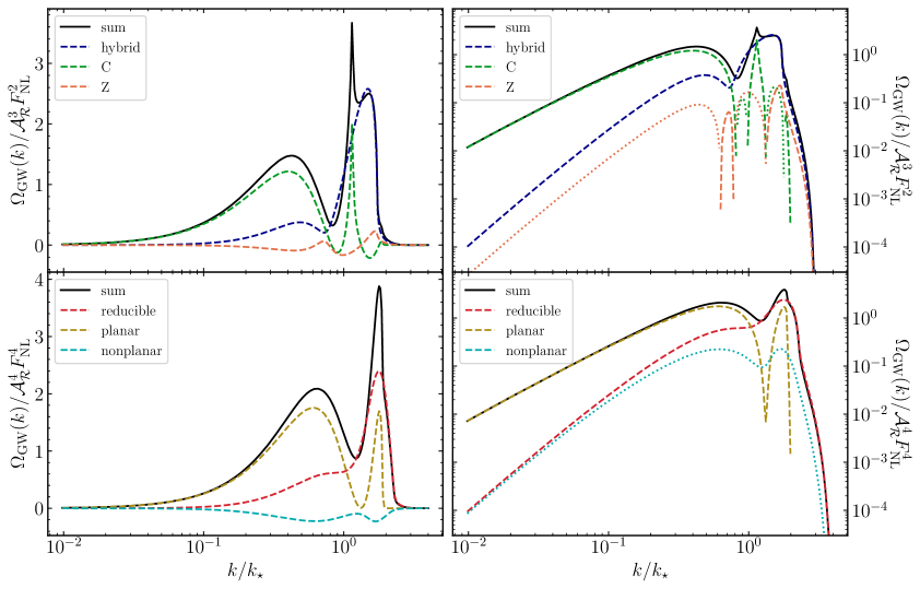
Figure 1: Unscaled (i.e., $\mathcal{A}_{\mathcal{R}}=1$ and $F_{\mathrm{NL}}=1$) non-Gaussian contributions for a monochromatic source, Eq. 3.1. The dashed lines indicate each contribution at $\mathcal{O}(F_{\mathrm{NL}}^{2})$ (top panels) and at $\mathcal{O}(F_{\mathrm{NL}}^{4})$ (bottom panels) with colors denoted in the legend. Solid black lines depict the sum of the individual contributions appearing in each panel. The left and right panels display the results on a linear and a log vertical scale, respectively. Because some individual contributions are negative at some $k$, dashed and dotted lines indicate where the sign is positive and negative, respectively.

Figure 1 displays the non-Gaussian contributions to the induced GW spectrum, dividing the $\mathcal{O}(F_{\mathrm{NL}}^{2})$ and $\mathcal{O}(F_{\mathrm{NL}}^{4})$ terms by $\mathcal{A}_{\mathcal{R}}^{3}F_{\mathrm{NL}}^{2}$ and $\mathcal{A}_{\mathcal{R}}^{4}F_{\mathrm{NL}}^{4}$, respectively. The connected terms clearly contribute as significantly as the disconnected ones, and they peak at differing wavenumbers. In particular, the C and planar terms are substantially larger in the infrared and also contribute comparably to the peaks at $k\gtrsim k_{\star}$. In contrast, the Z and nonplanar terms are smaller in magnitude. The C, Z, and nonplanar terms are (for at least some $k$) negative; however, as apparent in the right panels of Fig. 1, the summed contributions at each order in $F_{\mathrm{NL}}$ are positive definite.

By comparing the peak heights of the $\mathcal{O}(F_{\mathrm{NL}}^{2})$ and $\mathcal{O}(F_{\mathrm{NL}}^{4})$ terms in the left panels of Fig. 1, we can estimate at what value of $\mathcal{A}_{\mathcal{R}}F_{\mathrm{NL}}^{2}$ the two contributions are comparable. For instance, aside from the spike in the C term, the ratio of the peaks of the $\mathcal{O}(F_{\mathrm{NL}}^{2})$ and $\mathcal{O}(F_{\mathrm{NL}}^{4})$ contributions is roughly $1/2$. In the common range $\mathcal{A}_{\mathcal{R}}\sim 10^{-2}-10^{-3}$ considered for significant PBH production, for $F_{\mathrm{NL}}\sim 5-20$ the $\mathcal{O}(F_{\mathrm{NL}}^{4})$ terms contribute significantly. In the infrared (IR) limit, the ratios of the Gaussian and $\mathcal{O}(F_{\mathrm{NL}}^{2})$ contributions is roughly $0.43$, while that for the $\mathcal{O}(F_{\mathrm{NL}}^{2})$ and $\mathcal{O}(F_{\mathrm{NL}}^{4})$ ones is about $1.7$.

We investigate the relative contributions of the $\mathcal{O}(F_{\mathrm{NL}}^{2})$ and $\mathcal{O}(F_{\mathrm{NL}}^{4})$ terms in more detail in Fig. 2.

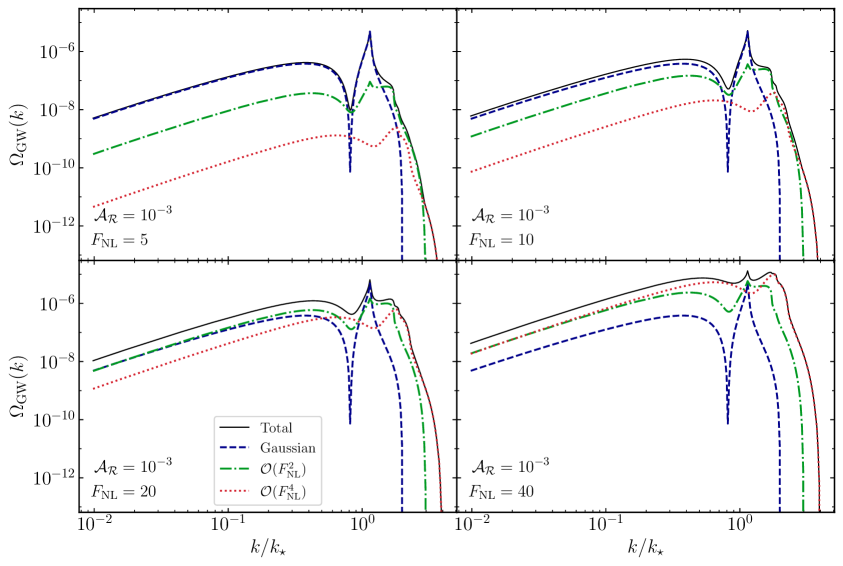
Figure 2: Induced GW spectrum after emission for a monochromatic source with $\mathcal{A}_{\mathcal{R}}=10^{-3}$ and various $F_{\mathrm{NL}}$. The Gaussian, $\mathcal{O}(F_{\mathrm{NL}}^{2})$, and $\mathcal{O}(F_{\mathrm{NL}}^{4})$ contributions appear in dashed blue, dot-dashed green, and dotted red respectively. The total spectrum is depicted in thin black.

We fix $\mathcal{A}_{\mathcal{R}}=10^{-3}$ and vary $F_{\mathrm{NL}}$ geometrically. For $F_{\mathrm{NL}}=5$ the Gaussian term dominates, but the non-Gaussian contributions produce “knees” near $k\sim 2k_{\star}$ and $3k_{\star}$ where the Gaussian contribution vanishes. At $F_{\mathrm{NL}}=10$ and $20$, the structure of the peak(s) is broadened by the $\mathcal{O}(F_{\mathrm{NL}}^{2})$ terms. Finally, at $F_{\mathrm{NL}}=40$ the $\mathcal{O}(F_{\mathrm{NL}}^{2})$ and $\mathcal{O}(F_{\mathrm{NL}}^{4})$ terms contribute comparably and dominate over the Gaussian one, resulting in a more complex peak. Note that much of this structure is smoother in more realistic scenarios with broader scalar power spectrum, as we investigate below.

As pointed out by Ref. [58], the infrared scaling of the induced GW spectrum includes a logarithmic running on top of the typical pure power law behavior. Though we verify that the spectral index of the disconnected non-Gaussian contributions may be approximated as $3+a\ln(bk)$ for some order-unity $a$ and $b$ (as found in Ref. [66]), of the connected terms this form only holds for the subdominant Z and nonplanar ones. The dominant non-Gaussian terms, the C and planar, scale with $k^{2+a\ln(bk)}$ like the Gaussian term [58]. As such, the spectral index of hypothetical GW signals could likely not be used to distinguish one dominated by Gaussian vs. non-Gaussian contributions. Furthermore, studies that neglect the connected terms significantly underestimate the non-Gaussian contributions to the GW spectrum in the IR.

To make contact with potential observations, Fig. 3 depicts the full, present-day GW signal alongside the sensitivity curves of various experiments [115].

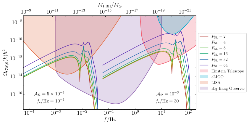
Figure 3: Present-day induced GW spectrum for a monochromatic source with various $F_{\mathrm{NL}}$, plotted against the sensitivity curves of various gravitational wave experiments [115, 116].

To get a sense of the sizes of PBHs that could possibly be produced in such scenarios, the top axis of Fig. 3 depicts the mass $M_{\mathrm{PBH}}$ of PBHs produced by the collapse of overdensities at horizon reentry on scales $k_{\star}=2\pi f_{\star}$ [48],

$$\frac{M_{\mathrm{PBH}}}{M_{\odot}} =\frac{\gamma}{0.2}\left(\frac{g_{\star}}{10.75}\right)^{-1/6}\left(\frac{f}{2.9\times 10^{-9}\,\mathrm{Hz}}\right)^{-2},$$ (3.3)

taking $\gamma=0.2$ and $g_{\star}=106.75$ for frequencies in and above the LISA band. We consider cases where $k_{\star}$ corresponds to a frequency of $10^{-2}\,\mathrm{Hz}$ in the LISA band and $30\,\mathrm{Hz}$ in the LIGO band. One can observe how the signal shape changes with $F_{\mathrm{NL}}$, with a distinctive three-peak structure arising at large $F_{\mathrm{NL}}$.

3.2 Lognormal spectrum

We now explore how the features of the GW spectrum induced by an idealized, monochromatic source are modulated when generalizing to a broader, more realistic spectrum. Consider a spectrum with a Gaussian bump in $\ln(k)$, as in, e.g., Ref. [88],

$$\Delta_{g}^{2}(k) =\frac{\mathcal{A}_{\mathcal{R}}}{\sqrt{2\pi\sigma^{2}}}\exp\left(-\frac{\ln^{2}(k/k_{\star})}{2\sigma^{2}}\right),$$ (3.4)

normalized so that $\int\mathrm{d}\ln k\,\Delta_{g}^{2}(k)=\mathcal{A}_{\mathcal{R}}$. In Fig. 4 we first study the effect of increasing $\sigma$ on each of the individual non-Gaussian contributions in turn.

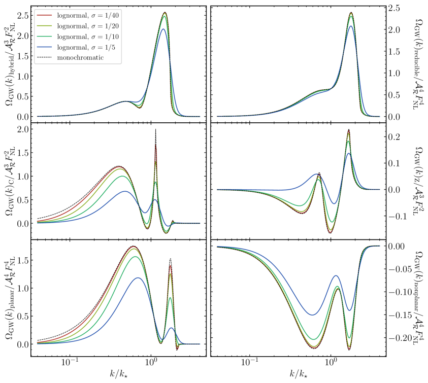
Figure 4: Unscaled (i.e., $\mathcal{A}_{\mathcal{R}}=1$ and $F_{\mathrm{NL}}=1$) non-Gaussian contributions for a lognormal source, Eq. 3.4. Solid lines depict results for $\sigma$ spanning $1/40$ through $1/5$ as indicated in the legend. The monochromatic result is overlaid in thin, dashed black.

As one might expect, the various features in each contribution become less pronounced, shrinking in amplitude and broadening in shape. In addition, most contributions exhibit a $k^{3+a\ln(bk)}$ scaling in the infrared. Only for the Gaussian, C, and planar terms does an intermediate regime of $k^{2+a\ln(bk)}$ behavior become partially evident for $\sigma=1/40$, but each transitions to $k^{3+a\ln(bk)}$ for $k/k_{\star}\lesssim 10^{-2}$.

We investigate the relative contributions of the $\mathcal{O}(F_{\mathrm{NL}}^{2})$ and $\mathcal{O}(F_{\mathrm{NL}}^{4})$ terms in more detail in Fig. 5, taking $\sigma=1/10$.

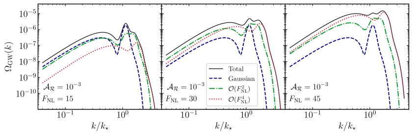
Figure 5: Induced GW spectrum after emission for a lognormal source with $\sigma=1/10$, $\mathcal{A}_{\mathcal{R}}=10^{-3}$ and various $F_{\mathrm{NL}}$. The Gaussian, $\mathcal{O}(F_{\mathrm{NL}}^{2})$, and $\mathcal{O}(F_{\mathrm{NL}}^{4})$ contributions appear in dashed blue, dot-dashed green, and dotted red respectively. The total spectrum is depicted in thin black.

We again fix $\mathcal{A}_{\mathcal{R}}=10^{-3}$ and vary $F_{\mathrm{NL}}$. The peak structure is smoothed compared to that for the monochromatic spectrum, Fig. 2. However, substantial non-Gaussianity does lead to a broad, nearly flat peak that distinguishes it from the narrower feature evident in the spectrum for a purely Gaussian curvature perturbation.

3.3 Gaussian-shaped spectrum

We next consider the Gaussian-bump spectrum used in Ref. [86],

$$\Delta_{g}^{2}(k) =\left(\frac{k}{k_{\star}}\right)^{3}\frac{\mathcal{A}_{\mathcal{R}}}{\sqrt{2\pi(\sigma/k_{\star})^{2}}}\exp\left(-\frac{(k-k_{\star})^{2}}{2\sigma^{2}}\right),$$ (3.5)

again normalized so that $\int\mathrm{d}\ln k\,\Delta_{g}^{2}(k)=\mathcal{A}_{\mathcal{R}}$. In Fig. 6 we show the total gravitational wave power spectrum for various values of the non-Gaussianity parameter, $F_{\mathrm{NL}}$. We compare results including and excluding the connected terms, choosing $\sigma=k_{\star}/30$, $\mathcal{A}_{\mathcal{R}}=10^{-3}$, and $f_{\star}=k_{\star}/2\pi=3\times 10^{-3}\,\mathrm{Hz}$ to match the choices of Ref. [86]. Even when neglecting the connected terms, we do not reproduce the particular peak structure observed in Ref. [86], and when including all contributions we observe a more pronounced second peak around $2f_{\star}$. Though the peak amplitude near $f_{\star}$ is largely unchanged, neglecting the connected term significantly underestimates the power at lower $k$ (as discussed in the monochromatic case above).

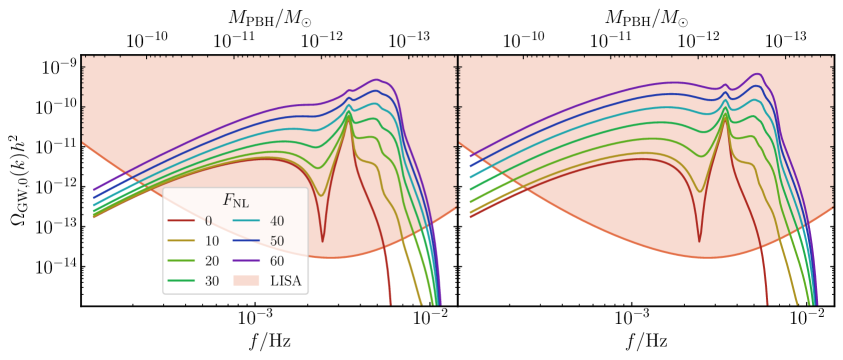
Figure 6: Gravitational wave spectra generated by a Gaussian-bump spectrum, Eq. 3.5, with $\sigma=k_{\star}/30$, $\mathcal{A}_{\mathcal{R}}=10^{-3}$, and $k_{\star}/2\pi=3\times 10^{-3}\,\mathrm{Hz}$. The left and right panels exclude and include the connected contributions, respectively.

3.4 Power law spectrum with an exponential cutoff

Another common spectral shape is a power law that is exponentially cut off near some $k_{\star}$,

$$\Delta_{g}^{2}(k) =\mathcal{A}_{\mathcal{R}}(k/k_{\star})^{\alpha}e^{-\alpha(k/k_{\star}-1)}.$$ (3.6)

This parameterization peaks at $k_{\star}$ with amplitude $\mathcal{A}_{\mathcal{R}}$ for any $\alpha$. For example, Ref. [111] found that, in contrast to the standard ultra slow roll scenario, an inflationary potential with a small step could generate a curvature spectrum with $\alpha=4$ and a peak amplitude as large as $\mathcal{A}_{\mathcal{R}}\approx 10^{-2}$. Equation 3.6 provides a good approximation to the result from Ref. [111], aside from the oscillations in $k$.

We display the individual results for each non-Gaussian term in Fig. 7.

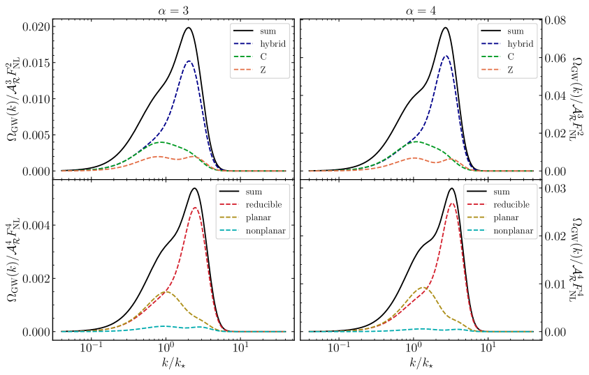
Figure 7: Unscaled (i.e., $\mathcal{A}_{\mathcal{R}}=1$ and $F_{\mathrm{NL}}=1$) non-Gaussian contributions for a power law source with an exponential cutoff, Eq. 3.6, for $\alpha=3$ (left panels) and $4$ (right panels). The dashed lines indicate each contribution at $\mathcal{O}(F_{\mathrm{NL}}^{2})$ (top panels) and at $\mathcal{O}(F_{\mathrm{NL}}^{4})$ (bottom panels) with colors denoted in the legend. Solid black lines depict the sum of the individual contributions appearing in each panel.

Like the monochromatic and lognormal sources, the connected and disconnected contributions peak at differing $k/k_{\star}$, but their sum (at each order in $F_{\mathrm{NL}}$) does not exhibit as prominent a multi-peak structure. The results are also not highly sensitive to the value of $\alpha$.

We again depict the contributions of the $\mathcal{O}(F_{\mathrm{NL}}^{2})$ and $\mathcal{O}(F_{\mathrm{NL}}^{4})$ terms for various $F_{\mathrm{NL}}$ in Fig. 8 for $\alpha=4$.

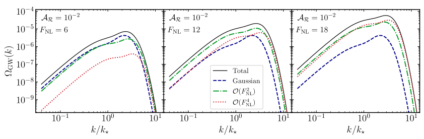
Figure 8: Induced GW spectrum after emission for a power law source with an exponential cutoff, Eq. 3.6, with $\alpha=4$, $\mathcal{A}_{\mathcal{R}}=10^{-2}$ and various $F_{\mathrm{NL}}$. The Gaussian, $\mathcal{O}(F_{\mathrm{NL}}^{2})$, and $\mathcal{O}(F_{\mathrm{NL}}^{4})$ contributions appear in dashed blue, dot-dashed green, and dotted red respectively. The total spectrum is depicted in thin black.

In contrast to sources that decay more quickly in the infrared, the shapes of the contributions to different orders in $F_{\mathrm{NL}}$ are similar, each exhibiting a relatively broad peak and an infrared scaling approaching $k^{3}$ with a moderate running. From the left panel of Fig. 8 we may deduce that the $\mathcal{O}(F_{\mathrm{NL}}^{2})$ contributions are comparable to the Gaussian one when $\mathcal{A}_{\mathcal{R}}F_{\mathrm{NL}}^{2}\approx 0.3$, while the right panel indicates that the $\mathcal{O}(F_{\mathrm{NL}}^{2})$ and $\mathcal{O}(F_{\mathrm{NL}}^{4})$ contributions match when $\mathcal{A}_{\mathcal{R}}F_{\mathrm{NL}}^{2}\approx 3$. However, the signal is cut off at larger $k/k_{\star}$ depending on whether (and which of) the non-Gaussian terms dominate.

Finally, we present results for the benchmark scenario of Ref. [111] (for the Gaussian part, including the effects of additional local-Gaussianity for illustrative purposes) in Fig. 9, with a peak frequency of $k_{\star}/2\pi=3\,\mathrm{nHz}$ and amplitude $\mathcal{A}_{\mathcal{R}}=10^{-2}$ (and $g_{\star}=10.75$).

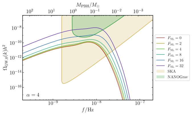
Figure 9: Present-day induced GW spectrum for a power law ($\alpha=4$) source with an exponential cutoff, setting $\mathcal{A}_{\mathcal{R}}=10^{-2}$. The shaded regions indicate the sensitivity curves for the pulsar timing experiments NANOGrav and the Square Kilometer Array (SKA) [115, 116].

3.5 Broken power law spectrum

We next study a broken power law spectrum, as considered in Ref. [74], with parameterization

$$\Delta_{g}^{2}(k) =\frac{\mathcal{A}_{\mathcal{R}}}{(k/k_{\star})^{-\alpha}+(k/k_{\star})^{\beta}},$$ (3.7)

scaling with $k^{\alpha}$ in the IR and $k^{-\beta}$ in the ultraviolet (UV). All contributions to the GW power exhibit a spectral index of $3+a\ln(bk)$ in the infrared as in the lognormal case in Section 3.2. In the ultraviolet the spectral index approaches $-2\beta$ for $0<\beta<4$ and $-4-\beta$ for $\beta>4$. These scalings agree with Ref. [74], which provided estimates of the IR and UV behavior for the hybrid and Z contributions. Aside from decaying as a power law in the UV rather than exponentially, the qualitative features of the induced GW spectrum for this case are similar to that for the exponentially cut off power law.

4 Conclusions

In this work we have carefully computed the effect of local non-Gaussianity on the spectrum of gravitational waves induced by scalar fluctuations. At lowest order in fluctuations, the induced gravitational wave spectrum is sourced by the trispectrum, or 4-point function of curvature fluctuations. We have shown that, contrary to some previous studies, the connected part of the trispectrum makes important contributions to the total spectrum that can neither be entirely neglected nor approximated by a multiple of the disconnected contributions. Our results demonstrate that studies of the induced GW spectrum from non-Gaussian curvature perturbations must carefully consider (and compute) all such contributions. For the power spectrum enhancements that are commonly considered in PBH scenarios (with $\mathcal{A}_{\mathcal{R}}\sim 10^{-3}$), even modest values of $F_{\mathrm{NL}}\sim\mathcal{O}(1)$ to $\mathcal{O}(10)$ significantly impact the induced GW spectrum.

A number of possible extensions merit attention. We have considered only the standard local-type non-Gaussianity, while more generally other bispectrum shapes may be relevant in detailed constructions, such as Ref. [111]. Furthermore, connected contributions must also be considered for higher-order non-Gaussianity, such as that considered in Ref. [66]. We leave these considerations for future work.

Appendix A Cosmological perturbation theory

In this appendix we elaborate on the dynamics of cosmological perturbations and the gravitational wave spectrum induced at second order by scalar perturbations. Recall that the background Einstein equations set

$$\mathcal{H}^{2} =\frac{a^{2}}{3m_{\mathrm{Pl}}^{2}}\mkern 1.25mu\overline{\mkern-1.25mu\rho\mkern-1.25mu}\mkern 1.25mu$$ (A.1a)

$$\mathcal{H}^{\prime}+\mathcal{H}^{2} =\frac{a^{2}}{6m_{\mathrm{Pl}}^{2}}\left(\mkern 1.25mu\overline{\mkern-1.25mu\rho\mkern-1.25mu}\mkern 1.25mu-3\mkern 1.25mu\overline{\mkern-1.25muP\mkern-1.25mu}\mkern 1.25mu\right).$$ (A.1b)

We define the perturbations to the stress-energy tensor as

$$\delta T^{0}_{\hphantom{0}0} =-\delta\rho$$ (A.2a)

$$\delta T^{0}_{\hphantom{0}i} =\left(\mkern 1.25mu\overline{\mkern-1.25mu\rho\mkern-1.25mu}\mkern 1.25mu+\mkern 1.25mu\overline{\mkern-1.25muP\mkern-1.25mu}\mkern 1.25mu\right)\partial_{i}\delta u$$ (A.2b)

$$\delta T^{i}_{\hphantom{i}j} =\delta_{ij}\delta P,$$ (A.2c)

neglecting vector and tensor perturbations and scalar anisotropic stress. We can solve the first-order Einstein equations for $\delta\rho$, $\delta P$, and $\delta u$ as

$$\delta\rho =-\frac{2m_{\mathrm{Pl}}^{2}}{a^{2}}\left(3\mathcal{H}\left(\Phi^{\prime}+\mathcal{H}\Phi\right)-\partial_{i}\partial_{i}\Phi\right)$$ (A.3a)

$$\delta P =\frac{6m_{\mathrm{Pl}}^{2}}{a^{2}}\left(\Phi^{\prime\prime}+3\mathcal{H}\Phi^{\prime}\right)-6\mkern 1.25mu\overline{\mkern-1.25muP\mkern-1.25mu}\mkern 1.25mu\Phi$$ (A.3b)

$$\delta u =-\frac{2m_{\mathrm{Pl}}^{2}}{a^{2}\left(\mkern 1.25mu\overline{\mkern-1.25mu\rho\mkern-1.25mu}\mkern 1.25mu+\mkern 1.25mu\overline{\mkern-1.25muP\mkern-1.25mu}\mkern 1.25mu\right)}\left(\Phi^{\prime}+\mathcal{H}\Phi\right).$$ (A.3c)

The terms in the space-space components of the Einstein tensor that are second order in the Newtonian potential are

$$a^{2}\delta^{(2)}G_{i}^{\hphantom{i}j} =4\Phi\partial_{i}\partial_{j}\Phi+2\partial_{i}\Phi\partial_{j}\Phi+\delta_{i}^{\hphantom{i}j}\left(20\left(\mathcal{H}^{2}+\mathcal{H}^{\prime}\right)\Phi^{2}+8\mathcal{H}\Phi\Phi^{\prime}-4\Phi\partial_{k}\partial_{k}\Phi-{\Phi^{\prime}}^{2}-3\partial_{k}\Phi\partial_{k}\Phi\right).$$ (A.4)

GWs are also sourced by second-order perturbations to the stress-energy tensor, which, using Eq. A.3, may be expressed in terms of metric perturbations as

$$\delta^{(2)}T_{i}^{\hphantom{i}j} =\frac{4m_{\mathrm{Pl}}^{4}}{a^{4}\left(\mkern 1.25mu\overline{\mkern-1.25mu\rho\mkern-1.25mu}\mkern 1.25mu+\mkern 1.25mu\overline{\mkern-1.25muP\mkern-1.25mu}\mkern 1.25mu\right)}\partial_{i}\left(\Phi^{\prime}+\mathcal{H}\Phi\right)\partial_{j}\left(\Phi^{\prime}+\mathcal{H}\Phi\right).$$ (A.5)

Dropping terms proportional to $\delta_{ij}$, setting $\mkern 1.25mu\overline{\mkern-1.25muP\mkern-1.25mu}\mkern 1.25mu=w\mkern 1.25mu\overline{\mkern-1.25mu\rho\mkern-1.25mu}\mkern 1.25mu$, and substituting Eq. A.1,

$$\mathcal{S}_{ij} =4\Phi\partial_{i}\partial_{j}\Phi+\frac{2(1+3w)}{3(1+w)}\partial_{i}\Phi\partial_{j}\Phi-\frac{4}{3(1+w)\mathcal{H}^{2}}\left[\partial_{i}\Phi^{\prime}\partial_{j}\Phi^{\prime}+\mathcal{H}\partial_{i}\Phi\partial_{j}\Phi^{\prime}+\mathcal{H}\partial_{i}\Phi^{\prime}\partial_{j}\Phi\right].$$ (A.6)

After using Eq. 2.13 to express the Newtonian potential in terms of the comoving curvature perturbation $\mathcal{R}(\mathbf{k})$ and the transfer function $\Phi(k\tau)$, taking a Fourier transform, and projecting onto (negative) $\epsilon^{\lambda}_{ij}(\mathbf{k})$, we find

$$\mathcal{S}_{\lambda}(\tau,\mathbf{k}) \equiv-\epsilon^{\lambda}_{lm}(\mathbf{k})\mathcal{S}_{lm}(\mathbf{k})$$ (A.7)

$$=\int\frac{\mathrm{d}^{3}q}{(2\pi)^{3/2}}Q_{\lambda}(\mathbf{k},\mathbf{q})f({\left|\mathbf{k}-\mathbf{q}\right|},q,\tau)\mathcal{R}(\mathbf{q})\mathcal{R}(\mathbf{k}-\mathbf{q}),$$ (A.8)

with

$$\begin{split}f(p,q,\tau)&\equiv\frac{3(1+w)}{(5+3w)^{2}}\bigg{[}2(5+3w)\Phi(p\tau)\Phi(q\tau)+\frac{4}{\mathcal{H}^{2}}\Phi^{\prime}(p\tau)\Phi^{\prime}(q\tau)\\ &\hphantom{{}={}\frac{3(1+w)}{(5+3w)^{2}}\Bigg{[}}+\frac{4}{\mathcal{H}}\left(\Phi(p\tau)\Phi^{\prime}(q\tau)+\Phi^{\prime}(p\tau)\Phi(q\tau)\right)\bigg{]}.\end{split}$$ (A.9)

Substituting $\mathcal{H}=\alpha/\tau$ (via Eq. 2.2) yields Eq. 2.15. The projection factors $Q_{\lambda}$ defined in Eq. 2.16 obey the symmetries

$$Q_{\lambda}(\mathbf{k},\mathbf{q}) =Q_{\lambda}(\mathbf{k},\mathbf{q}+\gamma\mathbf{k})$$ (A.10a)

$$Q_{\lambda}(\mathbf{k},\mathbf{q}) =Q_{\lambda}(-\mathbf{k},\mathbf{q})=Q_{\lambda}(\mathbf{k},-\mathbf{q})=Q_{\lambda}(-\mathbf{k},-\mathbf{q}).$$ (A.10b)

We next require the solution to the equation of motion of the transfer function, $\Phi(k\tau)$. In the absence of isocurvature perturbations, the Newtonian potential evolves according to

$$\Phi^{\prime\prime}(\tau,\mathbf{k})+3(1+w)\mathcal{H}\Phi^{\prime}(\tau,\mathbf{k})+wk^{2}\Phi(\tau,\mathbf{k}) =0,$$ (A.11)

after setting $\delta P=w\delta\rho$. Using Eq. 2.2, Eq. A.11 leads to

$$0 =\frac{\mathrm{d}^{2}\Phi}{\mathrm{d}y^{2}}+\frac{6(1+w)}{1+3w}\frac{1}{y}\frac{\mathrm{d}\Phi}{\mathrm{d}y}+\Phi,$$ (A.12)

where $y\equiv\sqrt{w}k\tau$. For $w\neq 0$, the solutions are given in terms of the spherical Bessel functions of the first and second kind, $j_{\nu}$ and $y_{\nu}$:

$$\Phi(k\tau) =\frac{C_{1}j_{\gamma-1}(y)+C_{2}y_{\gamma-1}(y)}{y^{\gamma-1}},$$ (A.13)

where $\gamma=3(1+w)/(1+3w)$. Imposing the superhorizon initial conditions $\Phi(x\to 0)=1$ and $\partial_{x}\Phi(x\to 0)=0$ sets $C_{1}=1$ and $C_{2}=0$. In radiation domination, $\gamma=2$ and

$$\Phi(y) =\frac{\sin y-y\cos y}{y^{3}}$$ (A.14)

In matter domination, the solution to Eq. A.11 for the transfer function is instead merely $\Phi(k\tau)=1.$

The Green function for the tensor perturbations (i.e., the solution to Eq. 2.20) is constructed via

$$G_{\mathbf{k}}(\tau,\mkern 1.25mu\overline{\mkern-1.25mu\tau\mkern-1.25mu}\mkern 1.25mu) =\frac{v_{1}(k\tau)v_{2}(k\mkern 1.25mu\overline{\mkern-1.25mu\tau\mkern-1.25mu}\mkern 1.25mu)-v_{1}(k\mkern 1.25mu\overline{\mkern-1.25mu\tau\mkern-1.25mu}\mkern 1.25mu)v_{2}(k\tau)}{v_{1}^{\prime}(k\mkern 1.25mu\overline{\mkern-1.25mu\tau\mkern-1.25mu}\mkern 1.25mu)v_{2}(k\mkern 1.25mu\overline{\mkern-1.25mu\tau\mkern-1.25mu}\mkern 1.25mu)-v_{1}(k\mkern 1.25mu\overline{\mkern-1.25mu\tau\mkern-1.25mu}\mkern 1.25mu)v_{2}^{\prime}(k\mkern 1.25mu\overline{\mkern-1.25mu\tau\mkern-1.25mu}\mkern 1.25mu)},$$ (A.15)

where $v_{1}$ and $v_{2}$ are the homogeneous solutions to the equation of motion for $v(k\tau)=a(\tau)h_{\lambda}(\tau,\mathbf{k})$,

$$\frac{\mathrm{d}^{2}v}{\mathrm{d}x^{2}}+\left(1-\frac{\alpha(\alpha-1)}{x^{2}}\right)v=0.$$ (A.16)

The solutions are

$$v_{1}(x) =xj_{\alpha-1}(x)$$ (A.17)

$$v_{2}(x) =xy_{\alpha-1}(x),$$ (A.18)

leading to

$$G_{\mathbf{k}}(\tau,\mkern 1.25mu\overline{\mkern-1.25mu\tau\mkern-1.25mu}\mkern 1.25mu) =k\tau\mkern 1.25mu\overline{\mkern-1.25mu\tau\mkern-1.25mu}\mkern 1.25mu\left[j_{\alpha-1}(k\mkern 1.25mu\overline{\mkern-1.25mu\tau\mkern-1.25mu}\mkern 1.25mu)y_{\alpha-1}(k\tau)-j_{\alpha-1}(k\tau)y_{\alpha-1}(k\mkern 1.25mu\overline{\mkern-1.25mu\tau\mkern-1.25mu}\mkern 1.25mu)\right].$$ (A.19)

In radiation domination where $w=1/3$ and so $\alpha=1$, the Green function is

$$G_{\mathbf{k}}(\tau,\mkern 1.25mu\overline{\mkern-1.25mu\tau\mkern-1.25mu}\mkern 1.25mu)=\frac{\sin k(\tau-\mkern 1.25mu\overline{\mkern-1.25mu\tau\mkern-1.25mu}\mkern 1.25mu)}{k}.$$ (A.20)

In, e.g., radiation domination, Eq. 2.22 can be computed analytically in terms of cosine and sine integrals via repeated integration by parts [53]. Defining $\tilde{I}(v,u,x)\equiv k^{2}I(vk,uk,x/k)$, the quantity required to compute the observable gravitational wave spectrum is

$$\begin{split}\mkern 1.25mu\overline{\mkern-1.25mu\tilde{I}(v_{1},u_{1},x\to\infty)\tilde{I}(v_{2},u_{2},x\to\infty)\mkern-1.25mu}\mkern 1.25mu&=\frac{1}{2x^{2}}\tilde{I}_{A}(u_{1},v_{1})\tilde{I}_{A}(u_{2},v_{2})\Big{[}\tilde{I}_{B}(u_{1},v_{1})\tilde{I}_{B}(u_{2},v_{2})\\ &\hphantom{{}={}\frac{1}{2x^{2}}\tilde{I}_{A}(u_{1},v_{1})\tilde{I}_{A}(u_{2},v_{2})\Big{[}}+\pi^{2}\tilde{I}_{C}(u_{1},v_{1})\tilde{I}_{C}(u_{2},v_{2})\Big{]},\end{split}$$ (A.21)

where

$$\tilde{I}_{A}(u,v) =\frac{3(u^{2}+v^{2}-3)}{4u^{3}v^{3}}$$ (A.22a)

$$\tilde{I}_{B}(u,v) =-4uv+(u^{2}+v^{2}-3)\ln{\left|\frac{3-(u+v)^{2}}{3-(u-v)^{2}}\right|}$$ (A.22b)

$$\tilde{I}_{C}(u,v) =\left(u^{2}+v^{2}-3\right)\Theta(v+u-\sqrt{3}).$$ (A.22c)

Appendix B Diagrammatic rules for the gravitational wave spectrum

In this appendix, we detail the computation of the contributions to the primordial trispectrum that induce gravitational waves. While a direct computation is straightforward, if tedious, we also present a diagrammatic representation of the non-Gaussian contributions. In order to make contact with existing literature, we present explicit Feynman-type rules with which one can represent each of the integrals contributing to the induced GW spectrum.

A complication in this approach is that the transfer functions relate the (nonlinear) curvature perturbation amplitudes to the Newtonian potential. The momenta flowing through the transfer functions must be tracked, and as we demonstrate below this leads to differences in diagrams that are otherwise topologically identical. We denote transfer functions with dashed lines; 3-momenta flow through these in the direction indicated by the arrow. The rules are given in Table 1. They function like regular Feynman rules: one draws all allowed diagrams and integrates over all loop momenta, momentum is conserved at each vertex, and the overall momentum of a diagram is zero.

(i)		$\displaystyle 4\int_{\tau_{0}}^{\tau}\mathrm{d}\mkern 1.25mu\overline{\mkern-1.25mu\tau\mkern-1.25mu}\mkern 1.25mu\,\frac{a(\mkern 1.25mu\overline{\mkern-1.25mu\tau\mkern-1.25mu}\mkern 1.25mu)}{a(\tau)}G_{\mathbf{k}}(\tau,\mkern 1.25mu\overline{\mkern-1.25mu\tau\mkern-1.25mu}\mkern 1.25mu)Q_{\lambda}(\mathbf{k},\mathbf{q})f({\left|\mathbf{k}-\mathbf{q}\right|},q,\mkern 1.25mu\overline{\mkern-1.25mu\tau\mkern-1.25mu}\mkern 1.25mu)$
(ii)		$1$
(iii)		$F_{\mathrm{NL}}$
(iv)		$\mathcal{P}_{g}(q)$

Table 1: Rules for the diagrammatic representation of Gaussian and local $F_{\mathrm{NL}}$-type non-Gaussian contributions to the induced GW spectrum. Wavy lines are gravitational waves, solid lines are (Gaussian) scalar power spectra, and dashed lines represent the transfer function of the Newtonian potential. Diagrams that include vertices in rule (iii) where the solid lines are connected into a loop vanish by virtue of the definition of $\mathcal{R}$ in Eq. 2.30.

Note that, even when performing the computations algebraically, a diagrammatic representation that accounts for the transfer functions facilitates determining the multiplicity of each term (while keeping in mind the symmetries of the transfer function and Eq. A.10).

The contribution from the purely Gaussian part of the curvature perturbation is shown in Fig. 10.

Figure 10: The Gaussian diagram, contributing at $\mathcal{O}(F_{\mathrm{NL}}^{0})$ to the GW power spectrum.

The contributions due to the non-Gaussianity of the curvature perturbation are shown in Fig. 11 for those at $\mathcal{O}(F_{\mathrm{NL}}^{2})$ and in Fig. 12 for those at $\mathcal{O}(F_{\mathrm{NL}}^{4})$. Contributions at higher order in $F_{\mathrm{NL}}$ require expanding the stress-energy tensor itself to higher order in fluctuations and are suppressed by additional powers of the amplitude of the curvature spectrum. We have omitted vanishing diagrams in which the solid lines in rule (iii) are connected; these simply cancel (see Eq. 2.30).

Figure 11: Hybrid (top left), Z (top right), and C (bottom left) diagrams, contributing at $\mathcal{O}(F_{\mathrm{NL}}^{2})$ to the GW power spectrum. The bottom right diagram vanishes due to the integration over the azimuthal angles of the internal momenta.

Figure 12: The reducible (top left), planar (top right), and nonplanar (bottom) diagrams, contributing at $\mathcal{O}(F_{\mathrm{NL}}^{4})$ to the GW power spectrum.

Compared to the diagrams in Ref. [88], we can identify the hybrid diagram in Fig. 11 and the disconnected, planar, and nonplanar ones in Fig. 12 by replacing our dashed lines with solid lines. However, the so-called “walnut” diagram of Ref. [88] could be either of the remaining diagrams in Fig. 11. No rules are provided in Ref. [88] for converting the diagrams to equations. However, our expression for the C diagram matches the expression for the “walnut” diagram in the supplemental material of Ref. [88]. (Furthermore, sans transfer functions, the propagator topology of the Z term more closely relates to the standard sunset diagram.)

Appendix C Recasting the integrals

In this appendix we recast the integrals into a numerically favorable form. Specifically, we present the polarization-summed, dimensionless gravitational wave power spectrum

$$\Delta_{h}^{2}(k) \equiv\frac{k^{3}}{2\pi^{2}}\sum_{\lambda}\mathcal{P}_{\lambda}(k).$$ (C.1)

First define the variables

$$u =\frac{{\left|\mathbf{k}-\mathbf{q}\right|}}{k}$$ (C.2)

$$v =\frac{q}{k}.$$ (C.3)

The Jacobian of this transformation is $-ku/v$, so the integration transforms to

$$\int\mathrm{d}^{3}q =k^{3}\int_{0}^{\infty}\mathrm{d}v\int_{\left|1-v\right|}^{1+v}\mathrm{d}u\,vu\int_{0}^{2\pi}\mathrm{d}\phi.$$ (C.4)

In terms of $u$ and $v$,

$$\sin^{2}\theta =\frac{4v^{2}-(1+v^{2}-u^{2})^{2}}{4v^{2}}.$$ (C.5)

Next define

$$s =u-v$$ (C.6)

$$t =u+v-1.$$ (C.7)

The Jacobian for this transformation is $1/2$, so

$$\int_{0}^{\infty}\mathrm{d}v\int_{{\left|1-v\right|}}^{1+v}\mathrm{d}u =\frac{1}{2}\int_{0}^{\infty}\mathrm{d}t\int_{-1}^{1}\mathrm{d}s.$$ (C.8)

The integration domain over $s$ and $t$ is rectangular, a requirement of most multidimensional numerical quadrature routines. Though these shall be our integration variables, we retain $u$ and $v$ in expressions for notational convenience.

Equation 2.22 takes the form

$$\tilde{I}(v,u,x)\equiv k^{2}I(q,{\left|\mathbf{k}-\mathbf{q}\right|},x/k) =\int_{x_{0}}^{x}\mathrm{d}\tilde{x}\,kG_{\mathbf{k}}(x/k,\tilde{x}/k)\frac{a(\tilde{x}/k)}{a(x/k)}f(vk,uk,\tilde{x}/k).$$ (C.9)

For further notational convenience, we define

$$\tilde{J}(v,u,x) \equiv v^{2}\sin^{2}\theta\tilde{I}(v,u,x)=\frac{4v^{2}-[1+v^{2}-u^{2}]^{2}}{4}\tilde{I}(v,u,x),$$ (C.10)

where $\theta$ is the polar angle of $\mathbf{q}$. Namely, $\tilde{J}(v,u,x)$ is equal to $\sqrt{2}Q_{\lambda}(\mathbf{k},\mathbf{q})I(q,{\left|\mathbf{k}-\mathbf{q}\right|},x/k)$ divided by $\sin 2\phi$ or $\cos 2\phi$ for the plus and cross polarizations, respectively.

C.1 Disconnected contributions

With the above definitions, the Gaussian contribution Eq. 2.33 to the (dimensionless) GW power spectrum (in terms of the dimensionless Gaussian curvature power spectrum $\Delta_{g}^{2}(k)$) is

$$\Delta_{h}^{2}(\tau,k)_{\mathrm{Gaussian}} =4\int_{0}^{\infty}\mathrm{d}t\int_{-1}^{1}\mathrm{d}s\,uv\tilde{J}(v,u,k\tau)^{2}\frac{\Delta_{g}(vk)}{v^{3}}\frac{\Delta_{g}(uk)}{u^{3}}.$$ (C.11)

Turning to the hybrid term, define

$$u_{1} =\frac{{\left|\mathbf{k}-\mathbf{q}_{1}\right|}}{k}$$ (C.12)

$$v_{1} =\frac{q_{1}}{k}$$ (C.13)

$$u_{2} =\frac{{\left|\mathbf{q}_{1}-\mathbf{q}_{2}\right|}}{q_{1}}$$ (C.14)

$$v_{2} =\frac{q_{2}}{q_{1}}.$$ (C.15)

Then Eq. 2.34 yields

$$\begin{split}\Delta_{h}^{2}(\tau,k)_{\mathrm{hybrid}}&=4F_{\mathrm{NL}}^{2}\int_{0}^{\infty}\mathrm{d}t_{1}\int_{-1}^{1}\mathrm{d}s_{1}\int_{0}^{\infty}\mathrm{d}t_{2}\int_{-1}^{1}\mathrm{d}s_{2}\,u_{1}v_{1}^{4}u_{2}v_{2}\\ &\hphantom{{}={}4F_{\mathrm{NL}}^{2}\int}\times\tilde{J}(v_{1},u_{1},k\tau)^{2}\frac{\Delta_{g}^{2}(u_{1}k)}{u_{1}^{3}}\frac{\Delta_{g}^{2}(v_{2}v_{1}k)}{(v_{2}v_{1})^{3}}\frac{\Delta_{g}^{2}(u_{2}v_{1}k)}{(u_{2}v_{1})^{3}}.\end{split}$$ (C.16)

Further defining

$$v_{3} =\frac{q_{3}}{{\left|\mathbf{k}-\mathbf{q}_{1}\right|}}$$ (C.17)

$$u_{3} =\frac{{\left|(\mathbf{k}-\mathbf{q}_{1})-\mathbf{q}_{3}\right|}}{{\left|\mathbf{k}-\mathbf{q}_{1}\right|}}.$$ (C.18)

the reducible term, Eq. 2.35, contributes as

$$\begin{split}\Delta_{h}^{2}(\tau,k)_{\mathrm{reducible}}&=F_{\mathrm{NL}}^{4}\int_{-1}^{1}\mathrm{d}s_{1}\int_{0}^{\infty}\mathrm{d}t_{1}\int_{-1}^{1}\mathrm{d}s_{2}\int_{0}^{\infty}\mathrm{d}t_{2}\int_{-1}^{1}\mathrm{d}s_{3}\int_{0}^{\infty}\mathrm{d}t_{3}\,u_{1}^{4}v_{1}^{4}u_{2}v_{2}u_{3}v_{3}\\ &\hphantom{{}={}F_{\mathrm{NL}}^{4}\int}\times\tilde{J}(v_{1},u_{1},k\tau)^{2}\frac{\Delta_{g}^{2}(v_{2}v_{1}k)}{(v_{2}v_{1})^{3}}\frac{\Delta_{g}^{2}(u_{2}v_{1}k)}{(u_{2}v_{1})^{3}}\frac{\Delta_{g}^{2}(v_{3}u_{1}k)}{(v_{3}u_{1})^{3}}\frac{\Delta_{g}^{2}(u_{3}u_{1}k)}{(u_{3}u_{1})^{3}}.\end{split}$$ (C.19)

C.2 Connected diagrams

For the connected diagrams we define

$$u_{i} =\frac{{\left|\mathbf{k}-\mathbf{q}_{i}\right|}}{k}$$ (C.20)

$$v_{i} =\frac{q_{i}}{k}$$ (C.21)

for all $i$. We require the dot products between various $\mathbf{q}_{i}$,

$$\begin{split}\frac{\mathbf{q}_{i}\cdot\mathbf{q}_{j}}{k^{2}}&=\frac{\cos(\phi_{i}-\phi_{j})}{4}\sqrt{t_{i}(t_{i}+2)(1-s_{i}^{2})t_{j}(t_{j}+2)(1-s_{j}^{2})}\\ &\hphantom{{}={}}+\frac{1}{4}\left[1-s_{i}(t_{i}+1)\right]\left[1-s_{j}(t_{j}+1)\right],\end{split}$$ (C.22)

as well as between $\mathbf{k}$ and $\mathbf{q}_{i}$:

$$\frac{\mathbf{k}\cdot\mathbf{q}_{i}}{k^{2}}=\frac{1}{2}\left[1-s_{i}(t_{i}+1)\right].$$ (C.23)

Because the integrands only depend on the differences between azimuthal angles, a suitable coordinate transformation renders one of the azimuthal integrals trivial. For the C and Z terms, Eqs. 2.36 and 2.37, we integrate over $\varphi=\phi_{1}-\phi_{2}$, leading to

$$\begin{split}\Delta_{h}^{2}(\tau,k)_{\mathrm{c},F_{\mathrm{NL}}^{2}}&=\frac{4F_{\mathrm{NL}}^{2}}{\pi}\prod_{i=1}^{2}\left[\int_{-1}^{1}\mathrm{d}s_{i}\int_{0}^{\infty}\mathrm{d}t_{i}\,u_{i}v_{i}\tilde{J}(u_{i},v_{i},k\tau)\right]\int_{0}^{2\pi}\mathrm{d}\varphi\,\cos 2\varphi\\ &\hphantom{{}={}\frac{4F_{\mathrm{NL}}^{2}}{\pi}}\times\left[\frac{\Delta_{g}^{2}(v_{2}k)}{v_{2}^{3}}\frac{\Delta_{g}^{2}(u_{2}k)}{u_{2}^{3}}\frac{\Delta_{g}^{2}(w_{a}k)}{w_{a}^{3}}+\frac{\Delta_{g}^{2}(v_{1}k)}{v_{1}^{3}}\frac{\Delta_{g}^{2}(v_{2}k)}{v_{2}^{3}}\frac{\Delta_{g}^{2}(w_{b}k)}{w_{b}^{3}}\right],\end{split}$$ (C.24)

where

$$w_{a}^{2} =v_{1}^{2}+v_{2}^{2}-2\frac{\mathbf{q}_{1}\cdot\mathbf{q}_{2}}{k^{2}}$$ (C.25)

$$w_{b}^{2} =1+v_{1}^{2}+v_{2}^{2}-2\frac{\mathbf{k}\cdot\mathbf{q}_{1}}{k^{2}}-2\frac{\mathbf{k}\cdot\mathbf{q}_{2}}{k^{2}}+2\frac{\mathbf{q}_{1}\cdot\mathbf{q}_{2}}{k^{2}}.$$ (C.26)

Finally, for the planar and nonplanar terms, Eqs. 2.38 and 2.39, we integrate over $\varphi_{12}\equiv\phi_{1}-\phi_{2}$ and $\varphi_{23}\equiv\phi_{2}-\phi_{3}$. We obtain

$$\begin{split}\Delta_{h}^{2}(\tau,k)_{\mathrm{c},F_{\mathrm{NL}}^{4}}&=\frac{F_{\mathrm{NL}}^{4}}{2\pi^{2}}\prod_{i=1}^{3}\left[\int_{-1}^{1}\mathrm{d}s_{i}\int_{0}^{\infty}\mathrm{d}t_{i}\,u_{i}v_{i}\right]\prod_{j=1}^{2}\left[\tilde{J}(u_{j},v_{j},k\tau)\right]\int_{0}^{2\pi}\mathrm{d}\varphi_{12}\mathrm{d}\varphi_{23}\,\cos 2\varphi_{12}\\ &\hphantom{{}={}\frac{F_{\mathrm{NL}}^{4}}{2\pi^{2}}}\times\left(\frac{\Delta_{g}^{2}(v_{3}k)}{v_{3}^{3}}\frac{\Delta_{g}^{2}(w_{13}k)}{w_{13}^{3}}\frac{\Delta_{g}^{2}(w_{23}k)}{w_{23}^{3}}\left[2\frac{\Delta_{g}^{2}(u_{3}k)}{u_{3}^{3}}+\frac{\Delta_{g}^{2}(w_{123}k)}{w_{123}^{3}}\right]\right),\end{split}$$ (C.27)

with the definitions

$$w_{i3}^{2} =v_{i}^{2}+v_{3}^{2}-\frac{2}{k^{2}}\mathbf{q}_{i}\cdot\mathbf{q}_{3}$$ (C.28)

$$\begin{split}w_{123}^{2}&=1+v_{1}^{2}+v_{2}^{2}+v_{3}^{2}-2\frac{\mathbf{k}\cdot\mathbf{q}_{1}}{k^{2}}-2\frac{\mathbf{k}\cdot\mathbf{q}_{2}}{k^{2}}+2\frac{\mathbf{k}\cdot\mathbf{q}_{3}}{k^{2}}\\ &\hphantom{{}={}}-2\frac{\mathbf{q}_{3}\cdot\mathbf{q}_{1}}{k^{2}}-2\frac{\mathbf{q}_{3}\cdot\mathbf{q}_{2}}{k^{2}}+2\frac{\mathbf{q}_{1}\cdot\mathbf{q}_{2}}{k^{2}}.\end{split}$$ (C.29)

We implement the integrals numerically with vegas+ [119], performing each for at least 200 external momenta $k$ and with a sufficiently large number of evaluations to achieve a relative precision of $10^{-3}$. For the higher dimensional integrals (the reducible and all connected terms), we find using a relatively short MCMC sample (implemented with emcee [123]) as a preconditioner to be an efficient means of generating an optimal vegas map (see the discussion in Ref. [119]).

Appendix D Monochromatic spectrum: infrared limit

We now sketch a derivation of the IR scaling of the induced GW spectrum for the monochromatic case, considering the C term [Eq. 2.36] as an example. Starting from Eq. C.24, changing integration variables from $\varphi$ to $c\equiv\cos\varphi$, and substituting Eq. 3.1,

$$\begin{split}\frac{\Delta_{h}^{2}(k,\tau)_{\mathrm{C{}}}}{F_{\mathrm{NL}}^{2}\mathcal{A}_{\mathcal{R}}^{3}}&=\frac{4}{\pi}\prod_{i=1}^{2}\left[\int_{-1}^{1}\mathrm{d}s_{i}\int_{0}^{\infty}\mathrm{d}t_{i}\,u_{i}v_{i}\tilde{J}(u_{i},v_{i},k\tau)\right]2\int_{-1}^{1}\mathrm{d}c\,\frac{2c^{2}-1}{\sqrt{1-c^{2}}}\\ &\hphantom{{}={}\frac{4}{\pi}}\times\frac{\delta(v_{1}\tilde{k}-1)}{v_{1}^{3}}\frac{\delta(u_{1}\tilde{k}-1)}{u_{1}^{3}}\frac{\delta(w_{a}\tilde{k}-1)}{w_{a}^{3}}.\end{split}$$ (D.1)

Recall that $\tilde{k}=k/k_{\star}$. Integrating the Dirac delta functions over $s_{1}$, $t_{1}$, and $c$ sets

$$s_{1} =0$$ (D.2a)

$$t_{1} =2/\tilde{k}-1$$ (D.2b)

$$c =\frac{-1+u_{2}^{2}+v_{2}^{2}}{4v_{1}v_{2}\sin\theta_{1}\sin\theta_{2}},$$ (D.2c)

and introduces a Jacobian factor of $2w_{a}/\tilde{k}^{3}v_{1}v_{2}\sin\theta_{1}\sin\theta_{2}$. Here $\theta_{i}$ is the azimuthal angle of $\mathbf{q}_{i}$, for which $\sin^{2}\theta_{i}=t_{i}(t_{i}+2)(1-s_{i}^{2})/4v_{i}^{2}$. Note that Eq. D.2 sets $v_{1}\sin\theta_{1}=\sqrt{1-\tilde{k}^{2}/4}/\tilde{k}$. The leading-order, IR behavior of the product of the (late-time, oscillation-averaged) transfer functions, Eq. A.21, resides in the $\tilde{I}_{A}\tilde{I}_{B}$ factors. After substituting Eq. C.10 for $\tilde{J}$ and evaluating $\tilde{I}_{A}(u_{1},v_{1})\tilde{I}_{B}(u_{1},v_{1})$ at $u_{1}=v_{1}=1/\tilde{k}$,

$$\begin{split}\frac{\Delta_{h}^{2}(k,\tau)_{\mathrm{C{}}}}{F_{\mathrm{NL}}^{2}\mathcal{A}_{\mathcal{R}}^{3}}&\approx\frac{12\tilde{k}^{4}}{2\pi(k\tau)^{2}}\ln\left(\frac{4}{3\tilde{k}^{2}}\right)\Theta(2-\tilde{k})\\ &\hphantom{{}={}}\times\int_{-1}^{1}\mathrm{d}s_{2}\int_{0}^{\infty}\mathrm{d}t_{2}\,\frac{2(2c^{2}-1)\Theta(1-{\left|c\right|})}{\sqrt{1-c^{2}}}\tilde{I}_{A}(u_{2},v_{2})\tilde{I}_{B}(u_{2},v_{2})u_{2}v_{2}^{2}\sin\theta_{2},\end{split}$$ (D.3)

where $c$ is implicitly set by Eq. D.2c.

The $\tilde{k}$-dependence of the remaining integral over $s_{2}$ and $t_{2}$ arises solely from $c$’s own $\tilde{k}$-dependence, affecting both the integrand and the bounds of integration via the Heaviside function $\Theta(1-{\left|c\right|})$. Inspecting the form of $c$ in Eq. D.2c (in terms of $s_{2}$ and $t_{2}$) shows that this Heaviside factor cuts off the integrals at $t_{2}\sim 4/\tilde{k}$. Furthermore, the integrand grows with $t_{2}$, so the integral is dominated by this upper limit. The integrand depends weakly on $s_{2}$ and one can show that regardless of $s_{2}$’s value, to leading order in $\tilde{k}$ and $1/t_{2}$ the $t_{2}$-dependence of the integrand is $\sim t_{2}\ln t_{2}$. As a result, the integral itself contributes a factor $\sim\tilde{k}^{-2}\ln\tilde{k}$ and so, to leading order in $\tilde{k}$,

$$\Omega_{\mathrm{GW},0}\sim\tilde{k}^{2}\ln^{2}\tilde{k}.$$ (D.4)

References

- [1] A. A. Starobinski, Spectrum of relict gravitational radiation and the early state of the universe, Soviet Journal of Experimental and Theoretical Physics Letters 30 (1979) 682.
- [2] A. H. Guth, Inflationary universe: A possible solution to the horizon and flatness problems, Phys. Rev. D 23 (1981) 347.
- [3] K. Sato, First Order Phase Transition of a Vacuum and Expansion of the Universe, Mon. Not. Roy. Astron. Soc. 195 (1981) 467.
- [4] V. F. Mukhanov and G. V. Chibisov, Quantum Fluctuations and a Nonsingular Universe, JETP Lett. 33 (1981) 532.
- [5] A. Linde, A new inflationary universe scenario: A possible solution of the horizon, flatness, homogeneity, isotropy and primordial monopole problems, Physics Letters B 108 (1982) 389.
- [6] A. Albrecht and P. J. Steinhardt, Cosmology for grand unified theories with radiatively induced symmetry breaking, Phys. Rev. Lett. 48 (1982) 1220.
- [7] A. D. Linde, Chaotic inflation, Physics Letters B 129 (1983) 177.
- [8] Planck collaboration, Planck 2018 results. VI. Cosmological parameters, Astron. Astrophys. 641 (2020) A6 [1807.06209].
- [9] BOSS collaboration, The clustering of galaxies in the completed SDSS-III Baryon Oscillation Spectroscopic Survey: cosmological analysis of the DR12 galaxy sample, Mon. Not. Roy. Astron. Soc. 470 (2017) 2617 [1607.03155].
- [10] D. M. Scolnic et al., The Complete Light-curve Sample of Spectroscopically Confirmed SNe Ia from Pan-STARRS1 and Cosmological Constraints from the Combined Pantheon Sample, Astrophys. J. 859 (2018) 101 [1710.00845].
- [11] Planck collaboration, Planck 2018 results. X. Constraints on inflation, Astron. Astrophys. 641 (2020) A10 [1807.06211].
- [12] G. Steigman, Primordial Nucleosynthesis in the Precision Cosmology Era, Ann. Rev. Nucl. Part. Sci. 57 (2007) 463 [0712.1100].
- [13] R. H. Cyburt, B. D. Fields, K. A. Olive and T.-H. Yeh, Big Bang Nucleosynthesis: 2015, Rev. Mod. Phys. 88 (2016) 015004 [1505.01076].
- [14] T. Kite, A. Ravenni, S. P. Patil and J. Chluba, Bridging the gap: spectral distortions meet gravitational waves, 2010.00040.
- [15] J. Chluba, J. Hamann and S. P. Patil, Features and New Physical Scales in Primordial Observables: Theory and Observation, Int. J. Mod. Phys. D 24 (2015) 1530023 [1505.01834].
- [16] T. Bringmann, P. Scott and Y. Akrami, Improved constraints on the primordial power spectrum at small scales from ultracompact minihalos, Phys. Rev. D 85 (2012) 125027 [1110.2484].
- [17] K. Ichikawa, M. Kawasaki and F. Takahashi, The Oscillation effects on thermalization of the neutrinos in the Universe with low reheating temperature, Phys. Rev. D 72 (2005) 043522 [astro-ph/0505395].
- [18] P. F. de Salas, M. Lattanzi, G. Mangano, G. Miele, S. Pastor and O. Pisanti, Bounds on very low reheating scenarios after Planck, Phys. Rev. D 92 (2015) 123534 [1511.00672].
- [19] T. Hasegawa, N. Hiroshima, K. Kohri, R. S. L. Hansen, T. Tram and S. Hannestad, MeV-scale reheating temperature and thermalization of oscillating neutrinos by radiative and hadronic decays of massive particles, JCAP 12 (2019) 012 [1908.10189].
- [20] K. Inomata and T. Nakama, Gravitational waves induced by scalar perturbations as probes of the small-scale primordial spectrum, Phys. Rev. D 99 (2019) 043511 [1812.00674].
- [21] G. Domènech, Induced gravitational waves in a general cosmological background, Int. J. Mod. Phys. D 29 (2020) 2050028 [1912.05583].
- [22] K. Inomata, K. Kohri, T. Nakama and T. Terada, Gravitational Waves Induced by Scalar Perturbations during a Gradual Transition from an Early Matter Era to the Radiation Era, JCAP 10 (2019) 071 [1904.12878].
- [23] K. Inomata, K. Kohri, T. Nakama and T. Terada, Enhancement of Gravitational Waves Induced by Scalar Perturbations due to a Sudden Transition from an Early Matter Era to the Radiation Era, Phys. Rev. D 100 (2019) 043532 [1904.12879].
- [24] F. Hajkarim and J. Schaffner-Bielich, Thermal History of the Early Universe and Primordial Gravitational Waves from Induced Scalar Perturbations, Phys. Rev. D 101 (2020) 043522 [1910.12357].
- [25] G. Domènech, S. Pi and M. Sasaki, Induced gravitational waves as a probe of thermal history of the universe, JCAP 08 (2020) 017 [2005.12314].
- [26] R. Allahverdi et al., The First Three Seconds: a Review of Possible Expansion Histories of the Early Universe, 2006.16182.
- [27] K. Tomita, Non-Linear Theory of Gravitational Instability in the Expanding Universe, Progress of Theoretical Physics 37 (1967) 831 [https://academic.oup.com/ptp/article-pdf/37/5/831/5234391/37-5-831.pdf].
- [28] S. Matarrese, O. Pantano and D. Saez, General-relativistic approach to the nonlinear evolution of collisionless matter, Phys. Rev. D 47 (1993) 1311.
- [29] S. Matarrese, O. Pantano and D. Saez, General relativistic dynamics of irrotational dust: Cosmological implications, Phys. Rev. Lett. 72 (1994) 320 [astro-ph/9310036].
- [30] S. Matarrese, S. Mollerach and M. Bruni, Second order perturbations of the Einstein-de Sitter universe, Phys. Rev. D 58 (1998) 043504 [astro-ph/9707278].
- [31] C. Carbone and S. Matarrese, A Unified treatment of cosmological perturbations from super-horizon to small scales, Phys. Rev. D 71 (2005) 043508 [astro-ph/0407611].
- [32] K. N. Ananda, C. Clarkson and D. Wands, The Cosmological gravitational wave background from primordial density perturbations, Phys. Rev. D 75 (2007) 123518 [gr-qc/0612013].
- [33] D. Baumann, P. J. Steinhardt, K. Takahashi and K. Ichiki, Gravitational Wave Spectrum Induced by Primordial Scalar Perturbations, Phys. Rev. D 76 (2007) 084019 [hep-th/0703290].
- [34] R. Saito and J. Yokoyama, Gravitational wave background as a probe of the primordial black hole abundance, Phys. Rev. Lett. 102 (2009) 161101 [0812.4339].
- [35] LISA collaboration, Laser Interferometer Space Antenna, arXiv e-prints (2017) arXiv:1702.00786 [1702.00786].
- [36] N. Seto, S. Kawamura and T. Nakamura, Possibility of direct measurement of the acceleration of the universe using 0.1-Hz band laser interferometer gravitational wave antenna in space, Phys. Rev. Lett. 87 (2001) 221103 [astro-ph/0108011].
- [37] K. Yagi and N. Seto, Detector configuration of DECIGO/BBO and identification of cosmological neutron-star binaries, Phys. Rev. D 83 (2011) 044011 [1101.3940].
- [38] M. Maggiore et al., Science Case for the Einstein Telescope, JCAP 03 (2020) 050 [1912.02622].
- [39] D. Reitze et al., Cosmic Explorer: The U.S. Contribution to Gravitational-Wave Astronomy beyond LIGO, Bull. Am. Astron. Soc. 51 (2019) 035 [1907.04833].
- [40] L. Lentati et al., European Pulsar Timing Array Limits On An Isotropic Stochastic Gravitational-Wave Background, Mon. Not. Roy. Astron. Soc. 453 (2015) 2576 [1504.03692].
- [41] L. Bian, R.-G. Cai, J. Liu, X.-Y. Yang and R. Zhou, On the gravitational wave sources from the NANOGrav 12.5-yr data, 2009.13893.
- [42] N. Aggarwal et al., Challenges and Opportunities of Gravitational Wave Searches at MHz to GHz Frequencies, 2011.12414.
- [43] E. Bugaev and P. Klimai, Induced gravitational wave background and primordial black holes, Phys. Rev. D 81 (2010) 023517 [0908.0664].
- [44] E. Bugaev and P. Klimai, Constraints on the induced gravitational wave background from primordial black holes, Phys. Rev. D 83 (2011) 083521 [1012.4697].
- [45] L. Alabidi, K. Kohri, M. Sasaki and Y. Sendouda, Observable Spectra of Induced Gravitational Waves from Inflation, JCAP 09 (2012) 017 [1203.4663].
- [46] L. Alabidi, K. Kohri, M. Sasaki and Y. Sendouda, Observable induced gravitational waves from an early matter phase, JCAP 05 (2013) 033 [1303.4519].
- [47] J. Garcia-Bellido, M. Peloso and C. Unal, Gravitational waves at interferometer scales and primordial black holes in axion inflation, JCAP 12 (2016) 031 [1610.03763].
- [48] K. Inomata, M. Kawasaki, K. Mukaida, Y. Tada and T. T. Yanagida, Inflationary primordial black holes for the LIGO gravitational wave events and pulsar timing array experiments, Phys. Rev. D 95 (2017) 123510 [1611.06130].
- [49] N. Orlofsky, A. Pierce and J. D. Wells, Inflationary theory and pulsar timing investigations of primordial black holes and gravitational waves, Phys. Rev. D 95 (2017) 063518 [1612.05279].
- [50] T. Nakama, J. Silk and M. Kamionkowski, Stochastic gravitational waves associated with the formation of primordial black holes, Phys. Rev. D 95 (2017) 043511 [1612.06264].
- [51] J. Garcia-Bellido, M. Peloso and C. Unal, Gravitational Wave signatures of inflationary models from Primordial Black Hole Dark Matter, JCAP 09 (2017) 013 [1707.02441].
- [52] G. Domènech and M. Sasaki, Hamiltonian approach to second order gauge invariant cosmological perturbations, Phys. Rev. D 97 (2018) 023521 [1709.09804].
- [53] K. Kohri and T. Terada, Semianalytic calculation of gravitational wave spectrum nonlinearly induced from primordial curvature perturbations, Phys. Rev. D 97 (2018) 123532 [1804.08577].
- [54] S. Clesse, J. García-Bellido and S. Orani, Detecting the Stochastic Gravitational Wave Background from Primordial Black Hole Formation, 1812.11011.
- [55] Z.-C. Chen, C. Yuan and Q.-G. Huang, Pulsar Timing Array Constraints on Primordial Black Holes with NANOGrav 11-Year Dataset, Phys. Rev. Lett. 124 (2020) 251101 [1910.12239].
- [56] A. Ota, Induced superhorizon tensor perturbations from anisotropic non-Gaussianity, Phys. Rev. D 101 (2020) 103511 [2001.00409].
- [57] Y.-F. Cai, C. Chen, X. Tong, D.-G. Wang and S.-F. Yan, When Primordial Black Holes from Sound Speed Resonance Meet a Stochastic Background of Gravitational Waves, Phys. Rev. D 100 (2019) 043518 [1902.08187].
- [58] C. Yuan, Z.-C. Chen and Q.-G. Huang, Log-dependent slope of scalar induced gravitational waves in the infrared regions, Phys. Rev. D 101 (2020) 043019 [1910.09099].
- [59] R.-G. Cai, S. Pi, S.-J. Wang and X.-Y. Yang, Pulsar Timing Array Constraints on the Induced Gravitational Waves, JCAP 10 (2019) 059 [1907.06372].
- [60] R.-G. Cai, S. Pi, S.-J. Wang and X.-Y. Yang, Resonant multiple peaks in the induced gravitational waves, JCAP 05 (2019) 013 [1901.10152].
- [61] N. Bartolo, D. Bertacca, V. De Luca, G. Franciolini, S. Matarrese, M. Peloso et al., Gravitational wave anisotropies from primordial black holes, JCAP 02 (2020) 028 [1909.12619].
- [62] S. Bhattacharya, S. Mohanty and P. Parashari, Primordial black holes and gravitational waves in nonstandard cosmologies, Phys. Rev. D 102 (2020) 043522 [1912.01653].
- [63] O. Özsoy and G. Tasinato, On the slope of the curvature power spectrum in non-attractor inflation, JCAP 04 (2020) 048 [1912.01061].
- [64] S. Pi and M. Sasaki, Gravitational Waves Induced by Scalar Perturbations with a Lognormal Peak, JCAP 09 (2020) 037 [2005.12306].
- [65] W.-T. Xu, J. Liu, T.-J. Gao and Z.-K. Guo, Gravitational waves from double-inflection-point inflation, Phys. Rev. D 101 (2020) 023505 [1907.05213].
- [66] C. Yuan and Q.-G. Huang, Gravitational waves induced by the local-type non-Gaussian curvature perturbations, 2007.10686.
- [67] G. Ballesteros, J. Rey, M. Taoso and A. Urbano, Primordial black holes as dark matter and gravitational waves from single-field polynomial inflation, JCAP 07 (2020) 025 [2001.08220].
- [68] J. Liu, Z.-K. Guo and R.-G. Cai, Analytical approximation of the scalar spectrum in the ultraslow-roll inflationary models, Phys. Rev. D 101 (2020) 083535 [2003.02075].
- [69] M. Braglia, D. K. Hazra, F. Finelli, G. F. Smoot, L. Sriramkumar and A. A. Starobinsky, Generating PBHs and small-scale GWs in two-field models of inflation, JCAP 08 (2020) 001 [2005.02895].
- [70] M. Braglia, X. Chen and D. K. Hazra, Probing Primordial Features with the Stochastic Gravitational Wave Background, JCAP 03 (2021) 005 [2012.05821].
- [71] J. Fumagalli, S. Renaux-Petel and L. T. Witkowski, Oscillations in the stochastic gravitational wave background from sharp features and particle production during inflation, 2012.02761.
- [72] A. D. Gow, C. T. Byrnes, P. S. Cole and S. Young, The power spectrum on small scales: Robust constraints and comparing PBH methodologies, JCAP 02 (2021) 002 [2008.03289].
- [73] F. Riccardi, M. Taoso and A. Urbano, Solving peak theory in the presence of local non-gaussianities, 2102.04084.
- [74] V. Atal and G. Domènech, Probing non-Gaussianities with the high frequency tail of induced gravitational waves, 2103.01056.
- [75] NANOGrav collaboration, The NANOGrav 12.5 yr Data Set: Search for an Isotropic Stochastic Gravitational-wave Background, Astrophys. J. Lett. 905 (2020) L34 [2009.04496].
- [76] V. Vaskonen and H. Veermäe, Did NANOGrav see a signal from primordial black hole formation?, Phys. Rev. Lett. 126 (2021) 051303 [2009.07832].
- [77] V. De Luca, G. Franciolini and A. Riotto, NANOGrav Data Hints at Primordial Black Holes as Dark Matter, Phys. Rev. Lett. 126 (2021) 041303 [2009.08268].
- [78] K. Kohri and T. Terada, Solar-Mass Primordial Black Holes Explain NANOGrav Hint of Gravitational Waves, Phys. Lett. B 813 (2021) 136040 [2009.11853].
- [79] S. Vagnozzi, Implications of the NANOGrav results for inflation, Mon. Not. Roy. Astron. Soc. 502 (2021) L11 [2009.13432].
- [80] G. Domènech and S. Pi, NANOGrav Hints on Planet-Mass Primordial Black Holes, 2010.03976.
- [81] S. Bhattacharya, S. Mohanty and P. Parashari, Implications of the NANOGrav result on primordial gravitational waves in nonstandard cosmologies, Phys. Rev. D 103 (2021) 063532 [2010.05071].
- [82] K. Inomata, M. Kawasaki, K. Mukaida and T. T. Yanagida, NANOGrav Results and LIGO-Virgo Primordial Black Holes in Axionlike Curvaton Models, Phys. Rev. Lett. 126 (2021) 131301 [2011.01270].
- [83] V. Atal, A. Sanglas and N. Triantafyllou, NANOGrav signal as mergers of Stupendously Large Primordial Black Holes, 2012.14721.
- [84] A. K. Pandey, Gravitational waves in neutrino plasma and NANOGrav signal, 2011.05821.
- [85] J. R. Espinosa, D. Racco and A. Riotto, A Cosmological Signature of the SM Higgs Instability: Gravitational Waves, JCAP 09 (2018) 012 [1804.07732].
- [86] R.-g. Cai, S. Pi and M. Sasaki, Gravitational Waves Induced by non-Gaussian Scalar Perturbations, Phys. Rev. Lett. 122 (2019) 201101 [1810.11000].
- [87] N. Bartolo, V. De Luca, G. Franciolini, M. Peloso, D. Racco and A. Riotto, Testing primordial black holes as dark matter with LISA, Phys. Rev. D 99 (2019) 103521 [1810.12224].
- [88] C. Unal, Imprints of Primordial Non-Gaussianity on Gravitational Wave Spectrum, Phys. Rev. D 99 (2019) 041301 [1811.09151].
- [89] C. Yuan, Z.-C. Chen and Q.-G. Huang, Probing primordial–black-hole dark matter with scalar induced gravitational waves, Phys. Rev. D 100 (2019) 081301 [1906.11549].
- [90] B. Carr, F. Kuhnel and M. Sandstad, Primordial Black Holes as Dark Matter, Phys. Rev. D 94 (2016) 083504 [1607.06077].
- [91] K. Inomata, M. Kawasaki, K. Mukaida, Y. Tada and T. T. Yanagida, Inflationary Primordial Black Holes as All Dark Matter, Phys. Rev. D 96 (2017) 043504 [1701.02544].
- [92] A. M. Green and B. J. Kavanagh, Primordial Black Holes as a dark matter candidate, J. Phys. G 48 (2021) 4 [2007.10722].
- [93] B. Carr, K. Kohri, Y. Sendouda and J. Yokoyama, Constraints on Primordial Black Holes, 2002.12778.
- [94] B. Carr and F. Kuhnel, Primordial Black Holes as Dark Matter: Recent Developments, Ann. Rev. Nucl. Part. Sci. 70 (2020) 355 [2006.02838].
- [95] M. Sasaki, T. Suyama, T. Tanaka and S. Yokoyama, Primordial black holes—perspectives in gravitational wave astronomy, Class. Quant. Grav. 35 (2018) 063001 [1801.05235].
- [96] C. Yuan and Q.-G. Huang, A topic review on probing primordial black hole dark matter with scalar induced gravitational waves, 2103.04739.
- [97] P. Adshead, R. Easther, J. Pritchard and A. Loeb, Inflation and the Scale Dependent Spectral Index: Prospects and Strategies, JCAP 1102 (2011) 021 [1007.3748].
- [98] P. H. Frampton, M. Kawasaki, F. Takahashi and T. T. Yanagida, Primordial Black Holes as All Dark Matter, JCAP 04 (2010) 023 [1001.2308].
- [99] M. Kawasaki, A. Kusenko and T. T. Yanagida, Primordial seeds of supermassive black holes, Phys. Lett. B 711 (2012) 1 [1202.3848].
- [100] M. M. Anber and L. Sorbo, Naturally inflating on steep potentials through electromagnetic dissipation, Phys. Rev. D 81 (2010) 043534 [0908.4089].
- [101] A. Linde, S. Mooij and E. Pajer, Gauge field production in supergravity inflation: Local non-Gaussianity and primordial black holes, Phys. Rev. D 87 (2013) 103506 [1212.1693].
- [102] E. Bugaev and P. Klimai, Axion inflation with gauge field production and primordial black holes, Phys. Rev. D 90 (2014) 103501 [1312.7435].
- [103] V. Domcke, F. Muia, M. Pieroni and L. T. Witkowski, PBH dark matter from axion inflation, JCAP 07 (2017) 048 [1704.03464].
- [104] M. A. G. Garcia, M. A. Amin and D. Green, Curvature Perturbations From Stochastic Particle Production During Inflation, JCAP 06 (2020) 039 [2001.09158].
- [105] O. Özsoy, Synthetic Gravitational Waves from a Rolling Axion Monodromy, JCAP 04 (2021) 040 [2005.10280].
- [106] O. Özsoy and Z. Lalak, Primordial black holes as dark matter and gravitational waves from bumpy axion inflation, JCAP 01 (2021) 040 [2008.07549].
- [107] P. Ivanov, P. Naselsky and I. Novikov, Inflation and primordial black holes as dark matter, Phys. Rev. D 50 (1994) 7173.
- [108] C. T. Byrnes, P. S. Cole and S. P. Patil, Steepest growth of the power spectrum and primordial black holes, JCAP 06 (2019) 028 [1811.11158].
- [109] O. Özsoy, S. Parameswaran, G. Tasinato and I. Zavala, Mechanisms for Primordial Black Hole Production in String Theory, JCAP 07 (2018) 005 [1803.07626].
- [110] H. V. Ragavendra, P. Saha, L. Sriramkumar and J. Silk, Primordial black holes and secondary gravitational waves from ultraslow roll and punctuated inflation, Phys. Rev. D 103 (2021) 083510 [2008.12202].
- [111] K. Inomata, E. Mcdonough and W. Hu, Primordial Black Holes Arise When The Inflaton Falls, 2104.03972.
- [112] C. T. Byrnes, E. J. Copeland and A. M. Green, Primordial black holes as a tool for constraining non-Gaussianity, Phys. Rev. D 86 (2012) 043512 [1206.4188].
- [113] S. Young and C. T. Byrnes, Primordial black holes in non-Gaussian regimes, JCAP 08 (2013) 052 [1307.4995].
- [114] G. Franciolini, A. Kehagias, S. Matarrese and A. Riotto, Primordial Black Holes from Inflation and non-Gaussianity, JCAP 03 (2018) 016 [1801.09415].
- [115] K. Schmitz, New Sensitivity Curves for Gravitational-Wave Signals from Cosmological Phase Transitions, JHEP 01 (2021) 097 [2002.04615].
- [116] K. Schmitz, New Sensitivity Curves for Gravitational-Wave Experiments, Feb., 2020. 10.5281/zenodo.3689582.
- [117] S. W. Hawking, Black hole explosions, Nature 248 (1974) 30.
- [118] S. W. Hawking, Particle Creation by Black Holes, Commun. Math. Phys. 43 (1975) 199.
- [119] G. P. Lepage, Adaptive Multidimensional Integration: VEGAS Enhanced, 2009.05112.
- [120] C. R. Harris, K. J. Millman, S. J. van der Walt, R. Gommers, P. Virtanen, D. Cournapeau et al., Array programming with NumPy, Nature 585 (2020) 357.
- [121] P. Virtanen, R. Gommers, T. E. Oliphant, M. Haberland, T. Reddy, D. Cournapeau et al., SciPy 1.0: Fundamental Algorithms for Scientific Computing in Python, Nature Methods 17 (2020) 261.
- [122] J. D. Hunter, Matplotlib: A 2d graphics environment, Computing in Science & Engineering 9 (2007) 90.
- [123] D. Foreman-Mackey, D. W. Hogg, D. Lang and J. Goodman, emcee: The MCMC Hammer, Publ. Astron. Soc. Pac. 125 (2013) 306 [1202.3665].