Variational Inference and Sparsity in High-Dimensional Deep Gaussian Mixture Models

Lucas Kock is PhD Student at Humboldt Universität zu Berlin. Nadja Klein is Assistant Professor and Emmy Noether Research Group Leader in Statistics and Data Science at Humboldt-Universität zu Berlin. David J. Nott is Associate Professor of Statistics and Applied Probability at National University of Singapore.
^∗ Correspondence should be directed to Prof. Dr. Nadja Klein at Humboldt Universität zu Berlin, Emmy Noether Research Group in Statistics and Data Science, Unter den Linden 6, 10099 Berlin, Germany. Email: nadja.klein@hu-berlin.de.

Acknowledgments: This work was supported by an NUS/BER Research Partnership grant by the National University of Singapore and Berlin University Alliance. Nadja Klein received support by the German research foundation (DFG) through the Emmy Noether grant KL 3037/1-1.

Gaussian mixture models are a popular tool for model-based clustering, and mixtures of factor analyzers are Gaussian mixture models having parsimonious factor covariance structure for mixture components. There are several recent extensions of mixture of factor analyzers to deep mixtures, where the Gaussian model for the latent factors is replaced by a mixture of factor analyzers. This construction can be iterated to obtain a model with many layers. These deep models are challenging to fit, and we consider Bayesian inference using sparsity priors to further regularize the estimation. A scalable natural gradient variational inference algorithm is developed for fitting the model, and we suggest computationally efficient approaches to the architecture choice using overfitted mixtures where unnecessary components drop out in the estimation. In a number of simulated and two real examples, we demonstrate the versatility of our approach for high-dimensional problems, and demonstrate that the use of sparsity inducing priors can be helpful for obtaining improved clustering results.

Keywords: Deep clustering; high-dimensional clustering; horseshoe prior; mixtures of factor analyzers; natural gradient; variational approximation.

1 Introduction

Exploratory data analysis tools such as cluster analysis need to be increasingly flexible to deal with the greater complexity of datasets arising in modern applications. For high-dimensional data, there has been much recent interest in deep clustering methods based on latent variable models with multiple layers. Our work considers deep Gaussian mixture models for clustering, and in particular a deep mixture of factor analyzers (DMFA) model recently introduced by Viroli and McLachlan (2019). The DMFA model is highly parametrized, and to make the estimation tractable Viroli and McLachlan (2019) consider a variety of constraints on model parameters which enable them to obtain promising results. The objective of the current work is to consider a Bayesian approach to estimation of the DMFA model which uses sparsity-inducing priors to further regularize the estimation. We use the horseshoe prior of Carvalho and Polson (2010), and demonstrate in a number of problems that the use of sparsity-inducing priors is helpful. This is particularly true in clustering problems which are high-dimensional and involve a large number of noise features. A computationally efficient natural gradient variational inference scheme is developed, which is scalable to high-dimensions and large datasets. A difficult problem in the application of the DMFA model is the choice of architecture, i.e. determining the number of layers and the dimension of each layer, since trying many different architectures is computationally burdensome. We discuss useful heuristics for choosing good models and selecting the number of clusters in a computationally thrifty way, using overfitted mixtures (Rousseau and Mengersen, 2011) with suitable priors on the mixing weights.

There are several suggested methods in the literature for constructing deep versions of Gaussian mixture models (GMM)s involving multiple layers of latent variables. One of the earliest is the mixture of mixtures model of Li (2005). Li (2005) considers modelling non-Gaussian components in mixture models using a mixture of Gaussians, resulting in a mixture of mixtures structure. The model is not identifiable through the likelihood, and Li (2005) suggests several ways to address this issue, as well as methods for choosing the number of components for each cluster. Malsiner-Walli et al. (2017) identify the model through the prior in a Bayesian approach, and consider Bayesian methods for model choice. Another deep mixture architecture is suggested in van den Oord and Schrauwen (2014). The authors consider a network with linear transformations at different layers, and the random sampling of a path through the layers. Each path defines a mixture component by applying the corresponding sequence of transformations to a standard normal random vector. Their approach allows a large number of mixture components, but without an explosion of the number of parameters due to the way parameters are shared between components.

The model of Viroli and McLachlan (2019) considered here is a multi-layered extension of the mixture of factor analyzers (MFA) model (Ghahramani and Hinton, 1997; McLachlan et al., 2003). The MFA model is a GMM in which component covariance matrices have a parsimonious factor structure, making this model suitable for high-dimensional data. The factor covariance structure can be interpreted as explaining dependence in terms of a low-dimensional latent Gaussian variable. Extending the MFA model to a deep model with multiple layers has two main advantages. First, non-Gaussian clusters can be obtained and second, it enables the fitting of GMMs with a large number of components, which is particularly relevant for high-dimensional data and cases when the number of true clusters is large. Tang et al. (2012) were the first to consider a deep MFA model, where a mixture of factor analyzers model is used as a prior for the latent factors instead of a Gaussian distribution. Applying this idea recursively leads to deep models with many layers. Their architecture splits components into several subcomponents at the next layer in a tree-type structure. Yang et al. (2017) consider a two layer version of the model of Tang et al. (2012) incorporating a common factor loading matrix at the first level and some other restrictions on the parametrization.

The model of Viroli and McLachlan (2019) combines some elements of the models of Tang et al. (2012) and van den Oord and Schrauwen (2014). Similar to Tang et al. (2012) an MFA prior is considered for the factors in an MFA model and multiple layers can be stacked together. However, similar to the model of van den Oord and Schrauwen (2014), their architecture has parameters for Gaussian component distributions with factor structure arranged in a network, with each Gaussian mixture component corresponding to a path through the network. Parameter sharing between components and the factor structure makes the model parsimonious. Viroli and McLachlan (2019) consider restrictions on the dimensionality of the factors at different layers and other model parameters to help identify the model. A stochastic EM algorithm is used for estimation, and they report improved performance compared to greedy layerwise fitting algorithms. For choosing the network architecture, they fit a large number of different architectures and use the Akaike Information Criterion (AIC) or Bayesian Information Criterion (BIC) to choose the final model. Selosse et al. (2020) report that even with the identification restrictions suggested in Viroli and McLachlan (2019) it can be very challenging to fit the DMFA model. The likelihood surface has a large number of local modes, and it can be hard to find good modes, possibly because the estimation of a large number of latent variables is difficult. This is one motivation for the sparsity priors we introduce here. While sparse Bayesian approaches have been considered before for both factor models (Carvalho et al. (2008); Ročková and George (2016); Hahn et al. (2018) among many others) and the MFA model (Ghahramani and Beal, 2000), they have not been considered for the DMFA model.

The structure of the paper is as follows. In Section 2 we introduce the DMFA model of Viroli and McLachlan (2019) and our Bayesian treatment making appropriate prior choices. Section 3 describes our scalable natural gradient variational inference method, and the approach to choice of the model architecture. Section 4 illustrates the good performance of our method for simulated data in a number of scenarios and compares our method to several alternative methods from the literature for simulated and benchmark datasets considered in Viroli and McLachlan (2019). Although it remains challenging to fit complex latent variable models such as the DMFA, we find that in many situations which are well-suited to sparsity our approach is helpful for producing better clusterings. Sections 5 and 6 consider two real high-dimensional examples on gene expression data and taxi networks illustrating the potential of our Bayesian treatment of DMFA models. Section 7 gives some concluding discussion.

2 Bayesian Deep Mixture of Factor Analyzers

This section describes our Bayesian DMFA model. We consider a conventional MFA model first in Section 2.1, and then the deep extension of this by Viroli and McLachlan (2019) in Section 2.2. The priors used for Bayesian inference are discussed in Section 2.3.

2.1 MFA model

In what follows we write $\operatorname{\mathcal{N}}(\mu,\Sigma)$ for the normal distribution with mean vector $\mu$ and covariance matrix $\Sigma$, and $\phi(y;\mu,\Sigma)$ for the corresponding density function. Suppose $y_{i}=(y_{i1},\dots,y_{id})^{\top}$, $i=1,\dots,n$ are independent identically distributed observations of dimension $d$. An MFA model for $y_{i}$ assumes a density of the form

$$\sum_{k=1}^{K}p_{k}\phi(y_{i};\mu_{k},B_{k}B_{k}^{\top}+\delta_{k}),$$ (1)

where $p_{k}>0$ are mixing weights, $k=1,\dots,K$, with $\sum_{k=1}^{K}p_{k}=1$; $\mu_{k}=(\mu_{k1},\dots,\mu_{kd})^{\top}$ are component mean vectors; and $B_{k}B_{k}^{\top}+\delta_{k}$, $k=1,\dots,K$, are component specific covariance matrices with $B_{k}$ $d\times D$ matrices, $D<<d$, and $\delta_{k}$ are $d\times d$ diagonal matrices with diagonal entries $(\delta_{k1},\dots,\delta_{kd})^{\top}$. The model (1) has a generative representation in terms of $D$-dimensional latent Gaussian random vectors, $z_{i}\sim\operatorname{\mathcal{N}}(0,I)$, $i=1,\dots,n$. Suppose that $y_{i}$ is generated with probability $p_{k}$ as

$$y_{i} =\mu_{k}+B_{k}z_{i}+\epsilon_{ik},$$ (2)

where $\epsilon_{ik}\sim\operatorname{\mathcal{N}}(0,\delta_{k})$. Under this generative model, $y_{i}$ has density (1). The latent variables $z_{i}$ are called factors, and the matrices $B_{k}$ are called factor loadings or factor loading matrices. In ordinary factor analysis (Bartholomew et al., 2011), which corresponds to $K=1$, restrictions on the factor loading matrices are made to ensure identifiability, and similar restrictions are needed in the MFA model. Common restrictions are lower-triangular structure with positive diagonal elements, or orthogonality of the columns of the factor loading matrix. With continuous shrinkage sparsity-inducing priors and careful initialization of the variational optimization algorithm, we did not find imposing an identifiability restriction such as a lower-triangular structure on the factor loading matrices to be necessary in our applications later. Identifiability issues for sparse factor models with point mass mixture priors have been considered recently in Frühwirth-Schnatter and Lopes (2018).

The MFA model is well-suited to analyzing high-dimensional data, because the modelling of dependence in terms of low-dimensional latent factors results in a parsimonious model. The idea of deep versions of the MFA model is to replace the Gaussian assumption $z_{i}\sim\operatorname{\mathcal{N}}(0,I)$ with the assumption that the $z_{i}$’s themselves follow an MFA model. This idea can be applied recursively, to define a deep model with many layers.

2.2 DMFA model

Suppose once again that $y_{i}$, $i=1,\dots,n$, are independent and identically distributed observations of dimension $D^{(0)}=d$, and define $y_{i}=z_{i}^{(0)}$. We consider a hierarchical model in which latent variables $z_{i}^{(l)}$, at layer $l=1,\dots,L$ are generated according to the following generative process. Let $K^{(l)}$ denote the number of mixture components at layer $l$. Then, with probability $p_{k}^{(l)}$, $k=1,\dots,K^{(l)}$, $\sum_{k}p_{k}^{(l)}=1$, $z_{i}^{(l-1)}$ is generated as

$$z_{i}^{(l-1)} =\mu_{k}^{(l)}+B_{k}^{(l)}z_{i}^{(l)}+\epsilon_{ik}^{(l)},$$ (3)

where $\epsilon_{ik}^{(l)}\sim\operatorname{\mathcal{N}}(0,\delta_{k}^{(l)})$, $\mu_{k}^{(l)}$ is a $D^{(l-1)}$-vector, $B_{k}^{(l)}$ is a $D^{(l-1)}\times D^{(l)}$ factor loading matrix, $\delta_{k}^{(l)}={\mbox{diag}}(\delta_{k1}^{(l)},\dots,\delta_{kD^{(l-1)}}^{(l)})$ is a $D^{(l-1)}\times D^{(l-1)}$ diagonal matrix with diagonal elements $\delta_{kj}^{(l)}>0$ and $z_{i}^{(L)}\sim\operatorname{\mathcal{N}}(0,I_{D^{(L)}})$. Eq. (3) is the same as the generative model (2) for $z_{i}^{(l-1)}$, except that we have replaced the Gaussian assumption for the factors appearing on the right-hand side with a recursive modelling using the MFA model. Write $\text{vec}(B_{k}^{(l)})$ for the vectorization of $B_{k}^{(l)}$, the vector obtained by stacking the elements of $B_{k}^{(l)}$ into a vector columnwise. Write

$$\begin{aligned} z^{(l)}&=({z_{1}^{(l)}}^{\top},\dots,{z_{n}^{(l)}}^{\top})^{\top},\\ \mu^{(l)}&=({\mu_{1}^{(l)}}^{\top},\dots,{\mu_{K^{(l)}}^{(l)}}^{\top})^{\top},\\ B^{(l)}&=({\text{vec}(B_{1}^{(l)})}^{\top},\dots,{\text{vec}(B_{K^{(l)}}^{(l)})}^{\top})^{\top},\\ \delta^{(l)}&=({\delta_{1}^{(l)}}^{\top},\dots,{\delta_{K^{(l)}}^{(l)}}^{\top})^{\top}\\ p^{(l)}&=(p_{1}^{(l)},\dots,p_{K^{(l)}}^{(l)})^{\top},\end{aligned}\qquad\begin{aligned} z&=({z^{(1)}}^{\top},\dots,{z^{(L)}}^{\top})^{\top},\\ \mu&=({\mu^{(1)}}^{\top},\dots,{\mu^{(L)}}^{\top})^{\top},\\ B&=({B^{(1)}}^{\top},\dots,{B^{(L)}}^{\top})^{\top},\\ \delta&=({\delta^{(1)}}^{\top},\dots,{\delta^{(L)}}^{\top})^{\top},\\ p&=({p^{(1)}}^{\top},\dots,{p^{(L)}}^{\top})^{\top}.\end{aligned}$$

In (3), we also denote $\gamma_{ik}^{(l)}=1$ if $z_{i}^{(l-1)}$ is generated from the $k$-th component model with probability $p_{k}^{(l)}$, $\gamma_{ik}^{(l)}=0$ otherwise, and

$$\gamma=({\gamma^{(1)}}^{\top},\dots,{\gamma^{(L)}}^{\top})^{\top},\;\;\;\gamma^{(l)}=({\gamma_{1}^{(l)}}^{\top},\dots,{\gamma_{n}^{(l)}}^{\top})^{\top},\;\;\;\gamma_{i}^{(l)}=(\gamma_{i1}^{(l)},\dots,\gamma_{iK^{(l)}}^{(l)})^{\top}.$$

Viroli and McLachlan (2019) observe that their DMFA model is just a Gaussian mixture model with $\prod_{l=1}^{L}K^{(l)}$ components. The components correspond to “paths” through the factor mixture components at the different levels. Write $k_{l}\in\{1,\dots,K^{(l)}\}$ for the index of a factor mixture component at level $l$. Let $k=(k_{1},\dots,k_{L})^{\top}$ index a path. Let $p(k)=\prod_{l=1}^{L}p_{k_{l}}^{(l)}$,

$$\mu(k)=\mu_{k_{1}}^{(1)}+\sum_{l=2}^{L}\left(\prod_{m=1}^{l-1}B_{k_{m}}^{(m)}\right)\mu_{k_{l}}^{(l)}\;\;\mbox{ and }\;\;\Sigma(k)=\delta_{k_{1}}^{(1)}+\sum_{l=2}^{L}\left(\prod_{m=1}^{l-1}B_{k_{m}}^{(m)}\right)\delta_{k_{l}}^{(l)}\left(\prod_{m=1}^{l-1}B_{k_{m}}^{(m)}\right)^{\top}.$$

Then the DMFA model corresponds to the Gaussian mixture density

$$\sum_{k}p(k)\phi(y;\mu(k),\Sigma(k)).$$

The DMFA allows expressive modelling through a large number of mixture components, but due to the parameter sharing and the factor structure the model remains parsimonious.

2.3 Prior distributions

For our priors on component mean parameters at each layer, we use heavy-tailed Cauchy priors, and for standard deviations, half-Cauchy priors. These thick-tailed priors tend to be dominated by likelihood information in the event of any conflict with the data. For component factor loading matrices, we use sparsity-inducing horseshoe priors. Sparse structure in factor loading matrices is motivated by the common situation where dependence can be explained through latent factors, where each one influences only a small subset of components. If the dependence structure is complex, it may be helpful to consider non-sparse factor loadings at the first layer, with higher levels of shrinkage in the prior at deeper layers where an elaborate modelling of dependence structure for the latent variables may be difficult to sustain.

Malsiner-Walli et al. (2017) consider a Bayesian approach to the mixture of mixtures model, which is a kind of DGMM, and give an interesting discussion of prior choice in that context. They observe that in the mixture of mixtures, the mixture at the higher level groups together the lower level clusters to accommodate non-Gaussianity, and their prior choices are constructed with this in mind. Unfortunately, the intuition behind their priors does not hold for the model considered here, since the network architecture of Viroli and McLachlan (2019) does not possess the nested structure of the mixture of mixtures, which is crucial to the prior construction in Malsiner-Walli et al. (2017).

A precise description of the priors will be given now. Denote the the complete vector of parameters by $\vartheta=(\mu^{\top},B^{\top},z^{\top},p^{\top},\delta^{\top},\gamma^{\top})^{\top}.$ First, we assume independence between $\mu$, $B$, $z$, $\delta$ and $p$ in their prior distribution. For the marginal prior distribution for $\mu$, we furthermore assume independence between all components, and the marginal prior density for $\mu_{kj}^{(l)}$ is assumed to be a Cauchy density, $\operatorname{\mathcal{C}}(0,G^{(l)})$, where $G^{(l)}$ is a known hyperparameter possibly depending on $l$, $l=1,\dots,L$. This Cauchy prior can be represented hierarchically as a mixture of a univariate Gaussian and inverse gamma distribution, i.e.

$$\mu_{kj}^{(l)}|g_{kj}^{(l)}\sim\operatorname{\mathcal{N}}(0,G^{(l)}g_{kj}^{(l)}),\;\;\;g_{kj}^{(l)}\sim\operatorname{\mathcal{IG}}\left(\frac{1}{2},\frac{1}{2}\right),$$

and we write

$$g=({g^{(1)}}^{\top},\dots,{g^{(L)}}^{\top})^{\top},\;\;\;g^{(l)}=({g_{1}^{(l)}}^{\top},\dots,{g_{K^{(l)}}^{(l)}}^{\top})^{\top}, g_{k}^{(l)}=(g_{k1}^{(l)},\dots,g_{kD^{(l-1)}}^{(l)})^{\top}.$$

We augment the model to include the parameters $g$ in this hierarchical representation.

For the prior on $B$, we assume elements are independently distributed a priori with a horseshoe prior (Carvalho and Polson, 2010),

$$\text{vec}(B_{k}^{(l)})_{j}\sim\operatorname{\mathcal{N}}\left(0,\tau_{k}^{(l)}/h_{kj}^{(l)}\right),\;\tau_{k}^{(l)}\sim\operatorname{\mathcal{IG}}\left(\frac{1}{2},\frac{1}{\xi_{k}^{(l)}}\right),\;\xi_{k}^{(l)}\sim\operatorname{\mathcal{IG}}\left(\frac{1}{2},\frac{1}{(\nu^{(l)})^{2}}\right),$$

$$h_{kj}^{(l)}\sim\operatorname{\mathcal{G}}\left(\frac{1}{2},c_{kj}^{(l)}\right),\;c_{kj}^{(l)}\sim\operatorname{\mathcal{G}}\left(\frac{1}{2},1\right),$$

where $\operatorname{\mathcal{G}}(a,b)$ denotes a gamma distribution with shape $a$ and scale parameter $b$ and we write

$$\begin{aligned} h&=({h^{(1)}}^{\top},\dots,{h^{(L)}}^{\top})^{\top},\\ c&=({c^{(1)}}^{\top},\dots,{c^{(L)}}^{\top})^{\top},\end{aligned}\qquad\begin{aligned} h^{(l)}&=({h_{1}^{(l)}}^{\top},\dots,{h_{K^{(l)}}^{(l)}}^{\top})^{\top},\\ c^{(l)}&=({c_{1}^{(l)}}^{\top},\dots,{c_{K^{(l)}}^{(l)}}^{\top})^{\top},\end{aligned}\qquad\begin{aligned} h_{k}^{(l)}&=(h_{k1}^{(l)},\dots,h_{k\kappa^{(l)}}^{(l)})^{\top},\\ c_{k}^{(l)}&=(c_{k1}^{(l)},\dots,c_{k\kappa^{(l)}}^{(l)})^{\top},\end{aligned}$$

$$\begin{aligned} \tau&=({\tau^{(1)}}^{\top},\dots,{\tau^{(L)}}^{\top})^{\top},\\ \xi&=({\xi^{(1)}}^{\top},\dots,{\xi^{(L)}}^{\top})^{\top},\end{aligned}\qquad\begin{aligned} \tau^{(l)}&=({\tau_{1}^{(l)}}^{\top},\dots,{\tau_{K^{(l)}}^{(l)}}^{\top})^{\top},\\ \xi^{(l)}&=({\xi_{1}^{(l)}}^{\top},\dots,{\xi_{K^{(l)}}^{(l)}}^{\top})^{\top},\end{aligned}$$

where $\kappa^{(l)}=D^{(l-1)}D^{(l)}$ and $\nu=({\nu^{(1)}}^{\top},\dots,{\nu^{(L)}}^{\top})^{\top}\in\text{$\mathds{R}$}^{L}$ are scale parameters assumed to be known. We augment the model to include the parameters $h,c,\tau,\xi$ in the hierarchical representation.

For $\delta$, we assume all elements are independent in the prior with $\sqrt{\delta_{kj}^{(l)}}$ being half-Cauchy distributed, $\sqrt{\delta_{kj}^{(l)}}\sim\operatorname{\mathcal{HC}}(A^{(l)})$, where the scale parameter $A^{(l)}$ is known and possibly depending on $l$, $l=1,\dots,L$. This prior can also be expressed hierarchically,

$$\delta_{kj}^{(l)}|\psi_{kj}^{(l)}\sim\operatorname{\mathcal{IG}}\left(\frac{1}{2},\frac{1}{\psi_{kj}^{(l)}}\right)\;\;\;\psi_{kj}^{(l)}\sim\operatorname{\mathcal{IG}}\left(\frac{1}{2},\frac{1}{{A^{(l)}}^{2}}\right),$$

and we write

$$\psi=({\psi^{(1)}}^{\top},\dots,{\psi^{(L)}}^{\top})^{\top},\;\;\;\psi^{(l)}=({\psi_{1}^{(l)}}^{\top},\dots,{\psi_{K^{(l)}}^{(l)}}^{\top})^{\top}, \psi_{k}^{(l)}=(\psi_{k1}^{(l)},\dots,\psi_{kD^{(l-1)}}^{(j)})^{\top}.$$

Once again, we can augment the original model to include $\psi$ and we do so.

The prior on $p$ assumes independence between $p^{(l)}$, $l=1,\dots,L$, and the marginal prior for $p^{(l)}$ is Dirichlet, $p^{(l)}\sim\mathpzc{Dir}(\rho_{1}^{(l)},\dots,\rho_{K^{(l)}}^{(l)})^{\top}$. The full set of unknowns in the model is $\{\mu,B,z,p,\delta,\gamma,p,\psi,g,h,c,\tau,\xi\}$ and we denote the corresponding vector of unknowns by

$$\theta =(\mu^{\top},\text{vec}(B)^{\top},z^{\top},p^{\top},\delta^{\top},\gamma^{\top},\psi^{\top},g^{\top},h^{\top},c^{\top},\tau^{\top},\xi^{\top})^{\top}.$$

3 Variational Inference for the Bayesian DMFA

Next we review basic ideas of variational inference and introduce a scalable variational inference method for the DMFA model.

3.1 Variational inference

Variational inference (VI) approximates a posterior density $p(\theta|y)$ by assuming a form $q_{\lambda}(\theta)$ for it and then minimizing some measure of closeness to $p(\theta|y)$. Here, $\lambda$ denotes variational parameters to be optimized, such as the mean and covariance matrix parameters in a multivariate Gaussian approximation. If the measure of closeness adopted is the Kullback-Leibler divergence, the optimal approximation maximizes the evidence lower bound (ELBO)

$$\mathcal{L}(\lambda)=\int q_{\lambda}(\theta)\log\left\{\frac{p(y,\theta)}{q_{\lambda}(\theta)}\right\}d\theta\,,$$ (4)

with respect to $\lambda$. Eq. (4) is an expectation with respect to $q_{\lambda}(\theta)$,

$$\mathcal{L}(\lambda)=\text{$\mathds{E}$}_{q_{\lambda}}\left\{\log(h(\theta))-\log(q_{\lambda}(\theta))\right\},\,$$ (5)

where $h(\theta)=p(y|\theta)p(\theta)$ and this observation enables an unbiased Monte Carlo estimation of the gradient of $\mathcal{L}(\lambda)$ after differentiating under the integral sign. This is often used with stochastic gradient ascent methods to optimize the ELBO, see Blei et al. (2017) for further background on VI methods. For some models and appropriate forms for $q_{\lambda}(\theta)$, ${\cal L}(\lambda)$ can be expressed analytically, and this is the case for our proposed VI method for the DFMA model. In this case, finding the optimal value $\lambda^{*}$ does not require Monte Carlo sampling from the approximation to implement the variational optimization (see e.g. Honkela et al., 2008), although the use of subsampling to deal with large datasets may still require the use of stochastic optimization.

3.2 Mean field variational approximation for DMFA

Choosing the form of $q_{\lambda}(\theta)$ requires balancing flexibility and computational tractability. Here we consider the factorized form

$$q_{\lambda}(\theta) =q(\mu)q(\text{vec}(B))q(z)q(p)q(\delta)q(\gamma)q(\psi)q(g)q(h)q(c)q(\tau)q(\xi).$$ (6)

and each factor in Eq. (6) will also be fully factorized. For the DMFA model, the existence of conditional conjugacy through our prior choices means that the parametric form of the factors follows from the factorization assumptions made. We can give an explicit expression for the ELBO (see the Web Appendix A.2 for details) and use numerical optimization techniques to find the optimal variational parameter $\lambda^{*}$. It is possible to consider less restrictive factorization assumptions than we have, retaining some of the dependence structure, while at the same time retaining the closed form for the lower bound. A fully factorized approximation has been used to reduce the number of variational parameters to optimize.

3.3 Approach to computations for large datasets

Optimization of the lower bound (5) with respect to the high-dimensional vector of variational parameters is difficult. One problem is that the number of variational parameters grows with the sample size. This occurs because we need to approximate posterior distributions of observation specific latent variables $z_{i}^{(l)}$ and $\gamma_{i}^{(l)}$, $i=1,\dots,n$, $l=1,\dots,L$. To address this issue, we adapt the idea of stochastic VI by Hoffman et al. (2013). More specifically, we split $\theta$ into so-called “global” and “local” parameters, $\theta=(\beta^{\top},\zeta^{\top})^{\top}$, where

$$\beta=(\mu^{\top},B^{\top},p^{\top},\delta^{\top},\psi^{\top},g^{\top},h^{\top},c^{\top},\tau^{\top},\xi^{\top})^{\top},$$

and $\zeta=(z^{\top},\gamma^{\top})^{\top}$ denote the “global” and “local” parameters of $\theta$, respectively.

We can similarly partition the variational parameters $\lambda$ into global and local components, $\lambda=(\lambda_{G}^{\top},\lambda_{L}^{\top})^{\top}$, where $\lambda_{G}$ and $\lambda_{L}$ are the variational parameters appearing in the variational posterior factors involving elements of $\beta$ and $\zeta$, respectively. Write the lower bound ${\cal L}(\lambda)$ as ${\cal L}(\lambda_{G},\lambda_{L})$. Write $M(\lambda_{G})$ for the value of $\lambda_{L}$ optimizing the lower bound with fixed global parameter $\lambda_{G}$. When optimizing ${\cal L}(\lambda)$, the optimal value of $\lambda_{G}$ maximizes

$$\overline{\cal L}(\lambda_{G}) ={\cal L}(\lambda_{G},M(\lambda_{G})).$$

Next, differentiate $\overline{\cal L}(\lambda_{G})$ to obtain

$$\nabla_{\lambda_{G}}\overline{\cal L}(\lambda_{G}) =\nabla_{\lambda_{G}}{\cal L}(\lambda_{G},M(\lambda_{G}))+\nabla_{\lambda_{G}}M(\lambda_{G})^{\top}\nabla_{M}{\cal L}(\lambda_{G},M(\lambda_{G}))$$

$$=\nabla_{\lambda_{G}}{\cal L}(\lambda_{G},M(\lambda_{G})).$$ (7)

The last line follows from $\nabla_{M}{\cal L}(\lambda_{G},M(\lambda_{G}))=0$, since $M(\lambda_{G})$ gives the optimal local variational parameter values for fixed $\lambda_{G}$. Eq. (7) says that the gradient $\nabla_{\lambda_{G}}\overline{\cal L}(\lambda_{G})$ can be computed by first optimizing to find $M(\lambda_{G})$, and then computing the gradient of ${\cal L}(\lambda)$ with respect to $\lambda_{G}$ with $\lambda_{L}$ fixed at $M(\lambda_{G})$.

We optimize $\overline{\cal L}(\lambda_{G})$ using stochastic gradient ascent methods, which iteratively update an initial value $\lambda_{G}^{(1)}$ for $\lambda_{G}$ for $t\geq 1$ by the iteration

$$\lambda_{G}^{(t+1)}=\lambda_{G}^{(t)}+a_{t}\circ\widehat{\nabla_{\lambda_{G}}\overline{\cal L}}(\lambda_{G}^{(t)}),$$

where $a_{t}$ is a vector-valued step size sequence, $\circ$ denotes elementwise multiplication, and $\widehat{\nabla_{\lambda_{G}}\overline{\cal L}}(\lambda_{G}^{(t)})$ is an unbiased estimate of the gradient of $\nabla_{\lambda_{G}}\overline{\cal L}(\lambda_{G})$ at $\lambda_{G}^{(t)}$. An unbiased estimator of (7) is constructed by randomly sampling a mini-batch of the data. This enables us to avoid dealing with all local variational parameters at once, lowering the dimension of any optimization. Let $A$ be a subset of $\{1,\dots,n\}$ chosen uniformly at random without replacement inducing the set of indices of a data mini-batch. Then, in view of (7), an unbiased estimate $\widehat{\nabla_{\lambda_{G}}\overline{\cal L}}(\lambda_{G})$ of ${\nabla_{\lambda_{G}}}\overline{\cal L}(\lambda_{G})$ can be obtained by

$$\widehat{\nabla_{\lambda_{G}}\overline{\cal L}}(\lambda_{G}) =\nabla_{\lambda_{G}}\mathcal{L}^{F}(\lambda_{G})+\frac{n}{|A|}\sum_{i\in A}\nabla_{\lambda_{G}}\mathcal{L}^{i}(\lambda_{G},M(\lambda_{G})),$$

where $|A|$ is the cardinality of $A$, and we have written ${\cal L}(\lambda)={\cal L}^{F}(\lambda_{G})+\sum_{i=1}^{n}{\cal L}^{i}(\lambda)$, where ${\cal L}^{i}(\lambda)$ is the contribution to ${\cal L}(\lambda)$ of all terms involving the local parameter for the $i$th observation and ${\cal L}^{F}(\lambda_{G})$ is the remainder. For this estimate, computation of all components of $M(\lambda_{G})$ is not required, since only the optimal local variational parameters for the mini-batch are needed.

To optimize $\lambda_{G}$ we use the natural gradient (Amari, 1998) rather than the ordinary gradient. The natural gradient uses an update which respects the meaning of the variational parameters in terms of the underlying distributions they index. The natural gradient is given by $I_{F}(\lambda_{G})^{-1}\widehat{\nabla_{\lambda_{G}}\overline{\cal L}}(\lambda_{G})$, where $I_{F}(\lambda_{G})=\text{Cov}(\nabla_{\lambda_{G}}q_{\lambda_{G}}(\beta))$, where $q_{\lambda_{G}}(\beta)$ is the $\beta$ marginal of $q_{\lambda}(\theta)$. Because of the factorization of the variational posterior into independent components, it suffices to compute the submatrices of $I_{F}(\lambda_{G})$ corresponding to each factor separately.

3.4 Algorithm

The complete algorithm can be divided into two nested steps iterating over the local and global parameters, respectively. First, an update of the global parameters is considered using a stochastic natural gradient ascent step for optimizing $\overline{\cal L}(\lambda_{G})$, with the adaptive stepsize choice proposed in Ranganath et al. (2013). For estimating the gradient in this step, the optimal local parameters $M(\lambda_{G})$ for the current $\lambda_{G}$ need to be identified for observations in a mini-batch. In theory, this can be done numerically by a gradient ascent algorithm. But this leads to a long run time, because one has to run this local gradient ascent until convergence for each step of the global stochastic gradient ascent. In our experience it is not necessary to calculate $M(\lambda_{G})$ exactly, and it suffices to use an estimate, which helps to decrease the run time of the algorithm. A natural approximate estimator for $M(\lambda_{G})$ can be constructed in the following way. Start by estimating the most likely path $\gamma_{i}$ using the clustering approach described in Section 3.6, while setting $\beta$ to the current variational posterior mean estimate for the global parameters. The local variational parameters appearing in the factor $q(z_{ij}^{(l)})$ are then estimated layerwise starting with $l=1$ by setting this density proportionally to $\exp(E(\log p(z_{ij}^{(l)}|z_{i}^{(l-1)},\gamma_{i},\beta)))$, where the expectation is with respect to $q(z_{ij}^{(l-1)})$, and which has a closed form Gaussian expression. In layer 1, $z_{i}^{(0)}=y_{i}$. The above approximation is motivated by the mean field update for $q(z_{ij})$, which is proportional to the exponential of the expected log full conditional for $z_{ij}^{(l)}$. However, the usual mean field update to do the local optimization would require iteration, which is why we use the fast layerwise approximation. The complete algorithm, details of the local optimization step and explicit expressions for the conditional $p(z_{ij}^{(l)}|z_{i}^{(l-1)},\gamma_{i},\beta)$ are given in the Web Appendix B.2. We calculate all gradients using the automatic differentiation of the Python package PyTorch (Paszke et al., 2017).

3.5 Hyperparameter choices

For all experiments we set the hyperparameters $G^{(l)}=2,\nu^{(l)}=1$ and $A^{(l)}=2.5$. The hyperparameter $\rho_{k}^{(l)}$ is set either to $1$ if the number of components in the respective layer is known, or to $0.5$ if the number of components is unknown, see Section 3.7 for further discussion. The size of the mini-batch is set to $5\%$ of the data size, but not less then 1 or larger then 1024. This way the number of variational parameters which need to be updated at every step remains bounded regardless of the sample size $n$.We found these hyperparameter choices to work well in all the diverse scenarios considered in Sections 4, 5 and 6.

3.6 Clustering with DMFA

The algorithm described in the previous section returns optimal variational parameters $\lambda_{G}$ for the global parameters $\beta$. A canonical point estimator for $\beta$ is then given by the mode of $q_{\lambda}(\theta)$. Following Viroli and McLachlan (2019), we consider only the first layer of the model for clustering. Specifically, the cluster of data point $y$ is given by

$$\operatorname*{{arg\,max}}_{k=1,\dots,K^{(1)}}p_{k}^{(1)}p(y|\beta,\gamma^{(1)}_{k}=1).$$

By integration over the local parameters for $y$, $p(y|\beta,\gamma^{(1)}_{k}=1)$ can be written as a mixture of $\prod_{r=2}^{L}K^{(r)}$ Gaussians of dimension $D^{(0)}$ for $k=1,\dots,K^{(1)}$. This way, the parameters of the bottom layers can be viewed as defining a density approximation to the different clusters and the overall model can be interpreted as a mixture of Gaussian mixtures. Alternatively, the DMFA can be viewed as a GMM with $\prod_{l=1}^{L}K^{(l)}$ components, where each component corresponds to a path through the model. By considering each of these Gaussian components as a separate cluster, the DMFA can be used to find a very large number of Gaussian clusters. However, Selosse et al. (2020) note that some of these “global” Gaussian components might be empty, even when there are data points assigned to every component in each layer. We investigate the idea of using the DMFA to fit a large scale GMM further in Section 6.

3.7 Model architecture and model selection

So far it has been assumed that the number of layers $L$, the number of components in each layer $K^{(l)}$, and the dimensions of each layer $D^{(l)}$, $l=1,\dots L$, are known. As this is usually not the case in practice, we now discuss how to choose a suitable architecture.

If the number of mixture components $K^{(l)}$ in a layer is unknown, we initialize the model with a relatively large number of components, and set the Dirichlet prior hyperparameters on the component weights to $\rho_{1}^{(l)}=\dots=\rho_{K}^{(l)}=0.5$. A large $K^{(l)}$ corresponds to an overfitted mixture, and for ordinary Gaussian mixtures unnecessary components will drop out under suitable conditions (Rousseau and Mengersen, 2011). A VI method for mixture models considering overfitted mixtures for model choice is discussed in McGrory and Titterington (2007). The results of Rousseau and Mengersen (2011) do not apply directly to deep mixtures because of the way parameters are shared between components, but we find that this method for choosing components is useful in practice. Our experiments show that in the case of deep Gaussian mixtures, the variational posterior concentrates around a small subset of components with high impact, while setting the weights for other components close to zero. Therefore, we remove all components with weights smaller than a threshold, set to be $0.01$ in simulations. After this, it is better in our experience to refit the model with the smaller number of components than to keep the fit initialized with the large number of components.

The choice of the number of layers $L$ and the dimensions $D$ is a classical model selection problem, where the model $m$ is chosen out of a finite set of proposed models in the model space $\mathcal{M}$. We assume a uniform prior on the model space $p(m)\propto 1$ for each $m\in\mathcal{M}$. Hence, the model can be selected by $\hat{m}=\operatorname*{{arg\,max}}_{m\in\mathcal{M}}p(m|y)=\operatorname*{{arg\,max}}_{m\in\mathcal{M}}p(y|m).$ Denoting the ELBO for the architecture $m$ with variational parameters $\lambda_{m}$ by $\mathcal{L}(\lambda_{m}|m)$, this is a lower bound for $\log p(y|m)$, which is tight if the variational posterior approximation is exact. Hence we choose the selected model by $\hat{m}=\operatorname*{{arg\,max}}_{m\in\mathcal{M}}\mathcal{L}(\lambda_{m}^{*}|m),$ where $\lambda_{m}^{*}$ denotes the optimal variational parameter value $\lambda_{m}$ for model $m$. Since it is computational expensive to run the VI algorithm until convergence for all models $m\in\mathcal{M}$, a naive approach would be to estimate $\mathcal{L}(\lambda_{m}^{*}|m)$ via $\mathcal{L}(\lambda_{m}^{(T)}|m)$ after running the algorithm for $T$ steps, where $\lambda_{m}^{(t)}$ is the value for $\lambda_{m}$ at iteration $t$. In our experiments we estimated $\mathcal{L}(\lambda_{m}^{*}|m)$ as the mean over the last $5\%$ of $250$ iterations, i.e. $\hat{m}=\operatorname*{{arg\,max}}_{m\in\mathcal{M}}\sum_{t=238}^{250}\mathcal{L}(\lambda_{m}^{(t)}|m).$ This calculation can be be parallelized by running the algorithm for each model $m$ on a different machine and only involves evaluations of the ELBO, which does not induce additional computational burden as the ELBO needs to be calculated for fitting the model. For the dimensions we test all possible choices fulfilling the Anderson-Rubin condition $D^{(l+1)}\leq\frac{D^{(l)}-1}{2}$ for $l=0,\dots,L$, which is a necessary condition for model identifiability (Frühwirth-Schnatter and Lopes, 2018). Additionally, this condition gives an upper bound for the number of layers. However, in our experiments, we consider only models with $L=2$ or $L=3$ layers, because in our experience architectures with few layers and a rapid decrease in dimension outperform architectures with many deep layers. Once an architecture is chosen based on short runs, the fitting algorithm is fully run to convergence for the optimal choice.

4 Benchmarking using simulated and real data

To demonstrate the advantages of our Bayesian DMFA with respect to clustering high-dimensional non-Gaussian data, computational efficiency of model selection, accommodating sparse structure and scalability to large datasets, we experiment on several simulated and publicly available benchmark examples.

4.1 Design of numerical experiments

First we consider two simulated datasets where our Bayesian approach with sparsity-inducing priors is able to outperform the maximum likelihood method considered in Viroli and McLachlan (2019). The data generating process for the first dataset scenario S1 is a GMM with many noisy (uninformative) features and sparse covariance matrices. Here, sparsity priors are helpful because there are many noise features. The data in scenario S2 has a similar structure to the real data from the application presented in Section 5 having unbalanced non-Gaussian clusters. Here, the true generative model has highly unbalanced group sizes, and the regularization that our priors provide is useful in this setting for stabilizing the estimation.

Five real datasets considered in Viroli and McLachlan (2019) are tested as well, and our method shows similar performance to theirs for these examples. However, we compare our method, which we will label VIdmfa, not only to the approach of Viroli and McLachlan (2019) (EMdgmm) but to several other benchmark methods, including a GMM based on the EM algorithm (EMgmm) and Bayesian VI approach by McGrory and Titterington (2007) (VIgmm), a skew-normal mixture (SNmm), a skew-t mixture (STmm), k-means (kmeans), partition around metroids (PAM), hierarchical clustering with Ward distance (Hclust), a factor mixture analyser (FMA) and a mixture of factor analyzer (MFA). To measure how close a set of clusters is to the ground truth labels, we consider three popular performance measures (e.g. Vinh et al. (2010)). These are the missclassification rate (MR), the adjusted rand index (ARI) and the adjusted mutual information (AMI).

4.2 Datasets

Below we describe the two simulated scenarios S1 and S2 involving sparsity, as well as the five real datasets used in Viroli and McLachlan (2019).
Scenario S1: Sparse location scale mixture. Datasets with $D^{(0)}=30$ features are drawn from a mixture of high-dimensional Gaussian distributions with sparse covariance structure. The first $15$ of the features yield information on the clusters and are obtained from a mixture of $K=5$ Gaussian distributions with different means $\mu_{k}$ and covariances $\Sigma_{k}$. The mean for component $k=1,\ldots,5$ has entries

$$(\mu_{k})_{j}=\begin{cases}-1&\mbox{ if $k$ divides $j$}\\ 1&\mbox{ otherwise,}\end{cases}$$

for $j=1,\dots,15$. The covariance matrices $\Sigma_{k}$ are drawn independently based on the Cholesky factors via the function make_sparse_spd_matrix from the Python package scikit-learn (Pedregosa et al., 2011). An entry of the Cholesky factros of $\Sigma_{k}$ is set to zero with a probability $\alpha=0.95$ and all non-zero entries are assumed to be in the interval $[0.4,0.7]$. The $15$ noise (irrelevant) features are drawn independently from an $\operatorname{\mathcal{N}}(0,1)$ distribution. The number of elements in each cluster is discrete uniformly distributed as $\operatorname{\mathcal{U}}\{50,200\}$ leading to datasets of sizes $n\in[250,1000]$. This clustering task is not as easy as it might first appear, since only half of the features contain any information on the class-labels.
Scenario S2: Cyclic data: We follow Yeung et al. (2001) and generate synthetic data modelling a sinusoidal cyclic behaviour of gene expressions over time. We simulate $n=235$ genes under $D^{(0)}=24$ experiments in $K=10$ classes. Two genes belong to the same class if they have similar phase shifts. Each element of the data matrix $y_{ij}$ with $i=1,\dots,n$ and $j=1,\dots,D^{(0)}$ is simulated as

$$y_{ij}=\delta_{j}+\lambda_{j}\left[\alpha_{i}+\beta_{i}\sin\left(\frac{2\pi j}{8}-\omega_{k}+\epsilon_{ij}\right)\right],$$

where $\alpha_{i}\sim\operatorname{\mathcal{N}}(0,1)$ represents the average expression level of gene $i$, $\beta_{i}\sim\mathcal{N}(3,0.5)$ is the amplitude control of gene $i$, $\lambda_{j}\sim\mathcal{N}(3,0.5)$ models the amplitude control of condition $j$, while the additive experimental error $\delta_{j}$ and the idiosyncratic noise $\epsilon_{ij}$ are drawn independently from $\mathcal{N}(0,1)$ distributions. The different classes are represented by $\omega_{k}$, $k=1,\ldots,K$, which are assumed to be uniformly distributed in $[0,2\pi]$, such that $\omega_{k}\sim\operatorname{\mathcal{U}}(0,2\pi)$. The sizes of the classes are generated according to Zipf’s law, meaning that gene $i$ is in class $k$ with probability proportional to $k^{-1}$. Each observation vector $y_{i}=(y_{i1},\ldots,y_{iD^{(0)}})^{\top}$ is individually standardized to have zero mean and unit variance. Recovering the class labels from the data can be difficult, because the classes are very unbalanced and some classes are very small. On average, only eight observations belong to cluster $k=10$. Furthermore, it is hard to distinguish between classes $k$ and $k^{\prime}$ if $\omega_{k}$ is close to $\omega_{k^{\prime}}$.
Wine data: The dataset from the R-package whitening (Strimmer et al., 2020) describes 27 properties of 178 samples of wine from three grape varieties (59 Barolo; 71 Grignolino; 48 Barbera) as reported in Forina et al. (1986).
Olive data: The dataset from the R-package cepp (Dayal, 2016) contains percentage composition of eight fatty acids found by lipid fraction of 572 Italian olive oils from three regions (323 Southern Italy; 98 Sardinia; 151 Northern Italy), see Forina et al. (1983).
Ecoli data: This dataset from (Dua and Graff, 2017) describes the amino acid sequences of 336 proteins using seven features provided by Horton and Nakai (1996). The class is the localization site (143 cytoplasm; 77 inner membrane without signal sequence; 52 perisplasm; 35 inner membrane, uncleavable signal sequence; 20 outer membrane; five outer membrane lipoprotein; two inner membrane lipoprotein; two inner membrane; cleavable signal sequence).
Vehicle data: This dataset from the R-package mlbench (Leisch and Dimitriadou, 2010) describes the silhouette of one of four types of vehicles, using a set of 19 features extracted from the silhouette. It consists of 846 observations (218 double decker bus; 199 Cherverolet van; 217 Saab 9000; 212 Opel manta 400).
Satellite data: This dataset from (Dua and Graff, 2017) consists of four digital images of the same scene in different spectral bands structured into a $3\times 3$ square of pixels defining the neighborhood structure. There are 36 pixels which define the features. We use all 6435 scenes (1533 red soil; 703 cotton crop; 1358 greysoil; 626 damp grey soil; 707 soil with vegetation stubble; 1508 very damp grey soil) as observations.
All real datasets are mean-centered and componentwise scaled to have unit variance.

4.3 Results

To compare the overall clustering performance we assume in a first step that the true number of clusters is known and fixed for all methods. Data-driven choice of the number of clusters is considered later. For Scenarios S1 and S2, $R=100$ datasets were independently generated. Boxplots of the ARI, AMI and MR across replicates are presented in Figure 1 for S1 and S2. Our method outperforms other approaches in both simulated scenarios. Even though the data generating process in Scenario S1 is a GMM, VIdmfa outperforms the classical GMM. One reason for this is that the data simulated in S1 is relatively noisy, and all information regarding the clusters is contained in a subspace smaller than the number of features. This is not only an assumption for VIdmfa, but also for FMA and MFA. However, compared to the latter two, VIdmfa is able to better recover the sparsity of the covariance matrices due to the shrinkage prior as Figure 2 demonstrates. The clusters derived by VIdmfa are Gaussian in this scenario, because the deeper layer has only one component. The data generating process of Scenario S2 is non-Gaussian and so are the clusters derived by VIdmfa, due to the fact that the deeper layer might have multiple components. The performance on the real data examples is summarized in Table 1. Here our approach is competitive with the other methods considered, but does not outperform the EMdgmm approach.

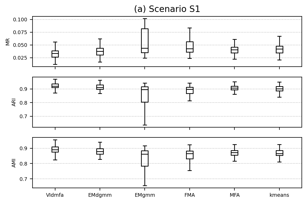
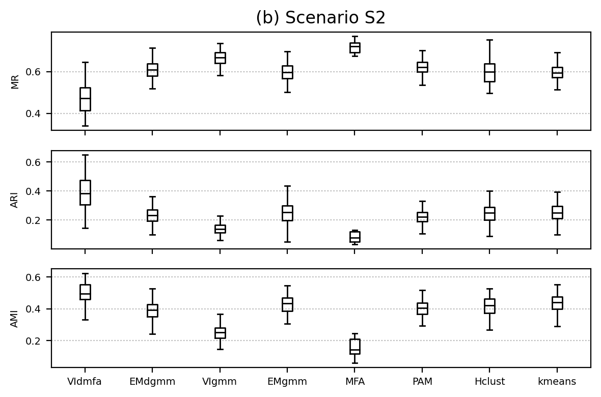
Figure 1: Scenario S1 (a) and Scenario S2 (b). Boxplots summarize row-wise the MR, ARI across $100$ replications. Here, we present only the best performing methods to make the plots more informative. A plot containing all benchmark methods and runs outside the interquartile range can be found in the Web Appendix C.3.

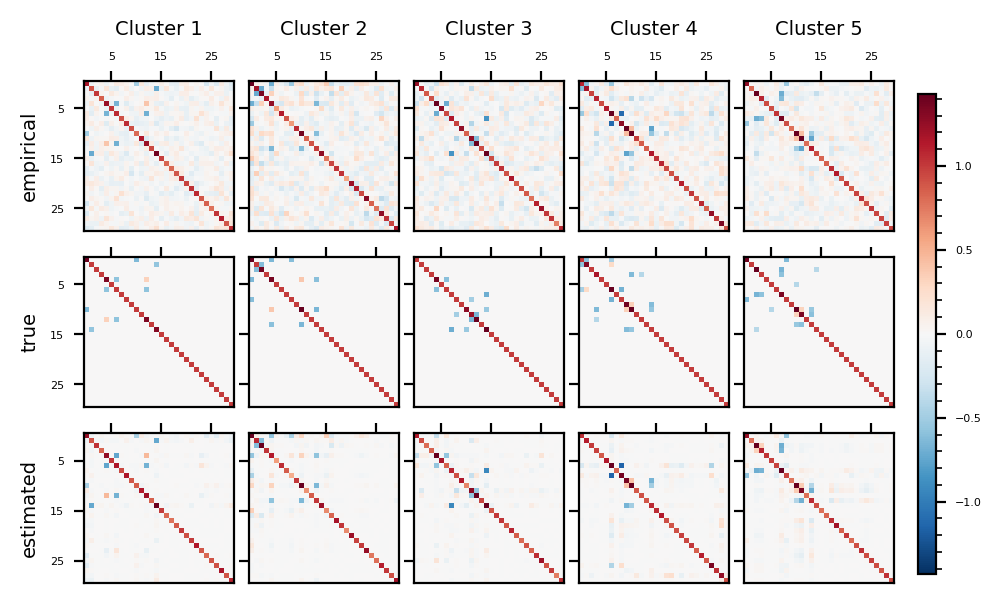
Figure 2: Scenario S1. Heat-maps of the true, the empirical and the estimated covariance matrices for each of the $5$ clusters. For the calculation of the empirical covariance matrices the true labels of the data points were used, which are not available in practice.

Wine Olive Ecoli Vehicle Satellite MR ARI AMI MR ARI AMI MR ARI AMI MR ARI AMI MR ARI AMI kmeans 0.022 0.930 0.900 0.234 0.448 0.584 0.351 0.508 0.626 0.642 0.076 0.112 0.321 0.530 0.612 PAM 0.045 0.863 0.818 0.107 0.725 0.673 0.333 0.507 0.608 0.628 0.073 0.097 0.313 0.531 0.608 Hclust 0.045 0.865 0.845 0.386 0.493 0.671 0.333 0.518 0.624 0.634 0.092 0.114 0.397 0.446 0.577 EMgmm 0.011 0.964 0.953 0.348 0.524 0.68 0.259 0.676 0.635 0.599 0.095 0.167 0.414 0.465 0.557 SNmm 0.511 0.048 0.047 0.108 0.854 0.769 - - - 0.506 0.224 0.371 0.435 0.414 0.535 STmm 0.427 0.194 0.218 0.098 0.864 0.785 0.298 0.594 0.571 0.476 0.207 0.314 0.390 0.468 0.543 FMA 0.011 0.965 0.946 0.495 0.235 0.406 0.411 0.44 0.485 - - - 0.439 0.435 0.516 MFA 0.006 0.983 0.973 0.052 0.914 0.855 - - - 0.573 0.153 0.201 0.226 0.622 0.666 VIgmm 0.494 0.074 0.055 0.000 1.000 1.000 0.357 0.478 0.476 0.522 0.198 0.286 0.460 0.445 0.525 EMdgmm 0.006 0.982 0.936 0.000 1.000 1.000 0.173 0.765 0.710 0.506 0.204 0.238 0.246 0.624 0.635 VIdmfa 0.006 0.982 0.973 0.000 1.000 1.000 0.202 0.726 0.688 0.499 0.208 0.354 0.390 0.449 0.546

Table 1: The MR, ARI and AMI for the real datasets rounded to three decimals is given and the best result is marked in each column. For each method the best out of $10$ runs (according either to BIC or the highest ELBO) is presented.

The assumption that the number of clusters is known is an artificial one. Clustering is often the starting point of the data investigation process and used to discover structure in the data. Selecting the number of clusters in those settings is sometimes a difficult task. In Bayesian mixture modelling this difficulty can be overcome by initializing the model with a relatively large number of components and using a shrinkage prior on the component weights, so that unnecessary components empty out (Rousseau and Mengersen, 2011). This is also the idea of our model selection process described in Section 3.7. To indicate that this is also a valid approach for VIdmfa, we fit both Scenarios S1, S2 for different choices of $K^{(0)}$ ranging from $2$ to $16$ and compare the average ARI and AMI over $10$ independent replicates. The results can be found in Figure 3. This suggests that our method is able to find the general structure of the data even when $K^{(0)}$ is larger than necessary, but the best results are derived when the model is initialized with the correct number of components. We have found it useful to fit the model with a potentially large number of components and then to refit the model with the number of components selected. This observation justifies our approach to selecting the number of components for the deeper layers discussed in Section 3.7. In both real data examples the optimal model architecture is unknown and VIdmfa selects a reasonable model.

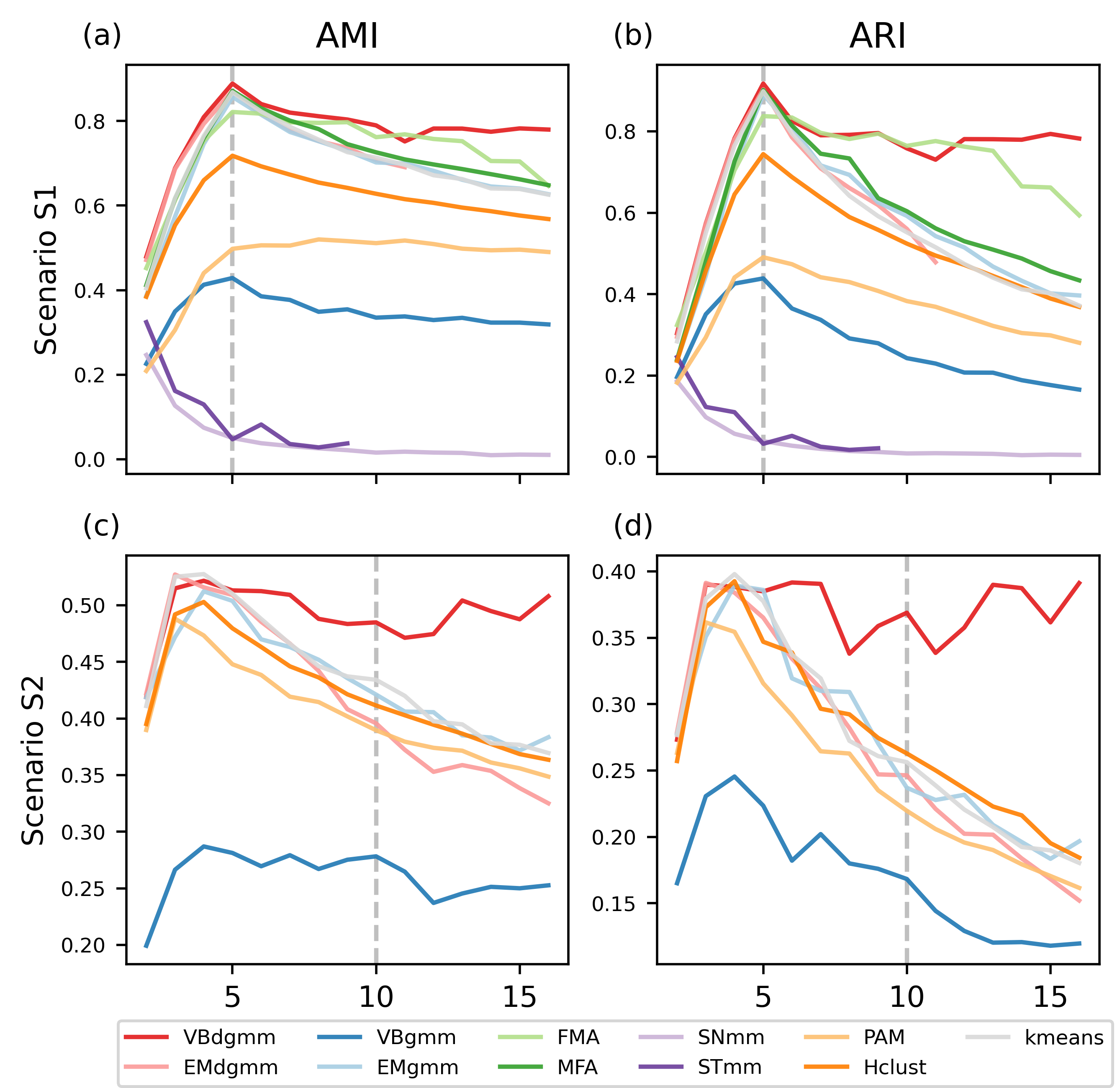
Figure 3: Scenario S1 (a, b) and Scenario S2 (c, d). The average AMI (a, c) and ARI (b, d) across $10$ independent replicates for different choices on the initial number of clusters $K=2,\dots,16$. The x-axis denotes the initialized number of clusters and the y-axis the average AMI/ARI. The optimal number of clusters for each data set is denoted by the dashed line.

5 Application to Gene Expression Data

In microarray experiments levels of gene expression for a large number of genes are measured under different experimental conditions. In this example we consider a time course experiment where the data can be represented by a real-valued expression matrix $\{m_{ij}$, $1\leq i\leq n$, $1\leq j\leq D\}$, where $m_{ij}$ is the expression level of gene $i$ at time $j$. We will consider rows of this matrix to be observations, so that we are clustering the genes according to the time series of their expression values.

Our model is well-suited to the analysis of gene expression datasets. In many time course microarray experiments both the number of genes and times is large, and our VIdmfa method scales well with both the sample size and dimension. If the time series expression profiles are smooth, their dependence may be well represented using low-rank factor structure. Our VIdmfa method also provides a computationally efficient mechanism for the choice of the number of mixture components. In the simulated Scenario S2 of Section 4, VIdmfa is able to detect unbalanced and comparable small clusters, which is the main advantage of our VIdmfa approach in comparison to the benchmark methods on this simulated gene expression data set and a similar behaviour is expected in real data applications.

As an example we consider the Yeast data set from Yeung et al. (2001), originally considered in Cho et al. (1998). This data set has been analyzed by many previous authors (Medvedovic and Sivaganesan, 2002; Tamayo et al., 1999; Lukashin and Fuchs, 2001) and contains $n=384$ genes over two cell cycles ($D=17$ time points) whose expression levels peak at different phases of the cell cycle. The goal is to cluster the genes according to those peaks and the structure is similar to the simulated cyclic data in Scenario S2 from Section 4. The genes were assigned to five cell cycle phases by Cho et al. (1998), but there are other cluster assignments with more groups available (Medvedovic and Sivaganesan, 2002; Lukashin and Fuchs, 2001). Hence, the optimal number of clusters for this data set is unknown and we aim to illustrate that our VIdmfa is able to select the number of clusters meaningfully. Also, the gene expression levels change relatively quickly between time points in this data set, suggesting a sparse correlation structure. VIdmfa is well suited for this scenario due to the sparsity inducing priors.

As in Scenario S2 and following Yeung et al. (2001), we individually scale each gene to have zero mean and unit variance. The simulation study in Section 4 suggests that VIdmfa can be initialized with a large number of potential components when the number of clusters is unknown, since the unnecessary components empty out. When initialized with $K^{(0)}=\lfloor\sqrt{n}\rfloor=19$ potential components, the model selection process described in Section 3.7 selects a model with $L=2$ layers with dimensions $D^{(1)}=4,D^{(2)}=1$ and $K^{(2)}=1$ components in the second layer. VIdmfa returns twelve clusters as shown in Figure 4. While some of the clusters are small, others are large and match well with the clusters proposed in Cho et al. (1998). For example, cluster eleven corresponds to their largest cluster. Comparisons to other kinds of information would be needed to decide if all of the twelve clusters are useful here, or if some of the clusters should be merged. For example, clusters two and twelve peak at similar phases of the cell cycle and could possibly be merged, while cluster nine does not seem to have a similar cluster and could be kept even though it contains only $n_{9}=6$ genes. An investigation of the fitted DMFA suggests that the clusters differ mainly by their means, while the covariance matrices have high sparsity, which matches with our expectation of (distant) time points being only weakly correlated.

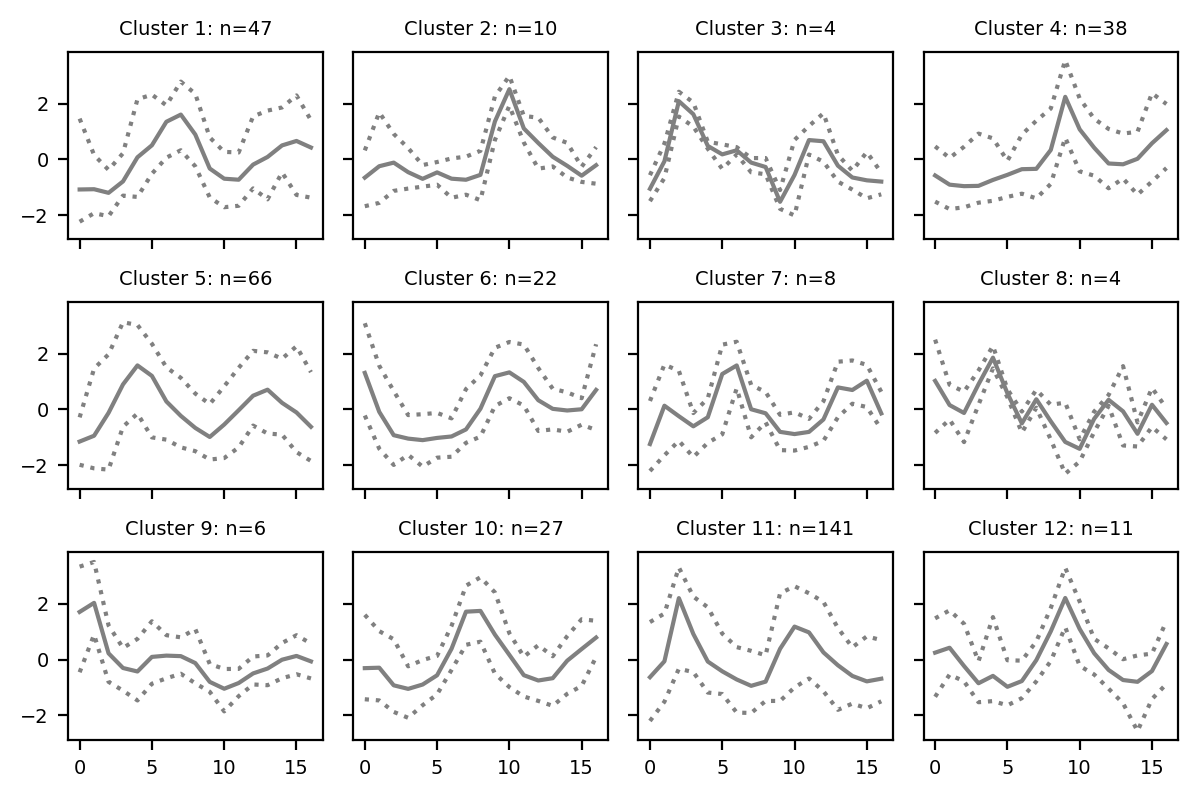
Figure 4: Yeast data. VIdmfa selects twelve clusters, when initialized with $K^{(0)}=19$. For each cluster the cluster mean (bold line), as well as minimum and maximum (dotted lines) on the normalized expression patterns are presented and $n$ denotes the number of elements in the respective cluster. The x-axis denotes the time and the y-axis labels the normalized gene expression.

6 Application to Taxi Trajectories

In this section, we consider a complex high-dimensional clustering problem for taxi trajectories. We use the publicly available data-set of Moreira-Matias et al. (2013) consisting of all busy trajectories from 01/07/2013 to 30/06/2014 performed by 442 taxis running in the city of Porto. Each taxi reports its coordinates at 15 second intervals. The dataset is large in dimension and sample size, with an approximate average of $50$ coordinates per trajectory and $1.7$ million observations in total. Understanding this dataset is a difficult task. Kucukelbir et al. (2017) propose a subspace clustering, where they project the data into an eleven-dimensional subspace using a extension on probabilistic principal component analysis in a first step and then use a GMM with 30 components to cluster the lower-dimensional data in a second step. This approach is successful in finding hidden structures in the data like busy roads and frequently taken paths. We will illustrate that VIdgmm is a good alternative because it does not require a separate dimension reduction step and is able to fit a GMM with a much larger number of components. Also VIdgmm scales well with the sample size, due to the sub-sampling approach described in Section 3.3.

In our analysis we focus on the paths of the trajectories ignoring the temporal dependencies and interpolate the data accordingly. Each trajectory $f_{i}$ can be viewed as a mapping $f_{i}(t):\{t_{0},\cdots,t_{T_{i}}\}\to\mathbb{R}^{2}$ of $T_{i}+1$ equally spaced time points onto coordinate pairs $(x_{i,t_{h}},y_{i,t_{h}})$ for $h=0,\cdots,T_{i}$ with $50$ time-points on average. We consider the interpolation $\tilde{f_{i}}:[0,1]\to\mathbb{R}^{2}$, where

$$\tilde{f_{i}}(t) =\sum_{h=0}^{T_{i}-1}\mathcal{I}{\left\{\frac{L_{i,h}}{L_{i,T_{i}}}\leq t\leq\frac{L_{i,h+1}}{L_{i,T_{i}}}\right\}}(t)\left[\left(1-\frac{t-\frac{L_{i,h}}{L_{i,T_{i}}}}{\frac{L_{i,h+1}}{L_{i,T_{i}}}-\frac{L_{i,h}}{L_{i,T_{i}}}}\right)f_{i}(t_{h})+\frac{t-\frac{L_{i,h}}{L_{i,T_{i}}}}{\frac{L_{i,h+1}}{L_{i,T_{i}}}-\frac{L_{i,h}}{L_{i,T_{i}}}}f_{i}(t_{h+1})\right],$$

and $L_{i,h}=\sum_{s=0}^{h-1}||f_{i}(t_{s})-f_{i}(t_{s+1})||$ is the length of the trajectory up to time-point $t_{h}$. This interpolation is time-independent in the sense that $d(\tilde{f_{i}}(t),\tilde{f_{i}}(t+\delta))$ is linear in $t$ for all $\delta>0$, where $d_{i}(\cdot,\cdot)$ denotes the distance between two points along a linear interpolation of the trajectory $f_{i}$. This way two trajectories $f_{i}$ and $f_{i^{\prime}}$ with the same path, i.e. the same image in $\mathbb{R}^{2}$, have similar interpolations $\tilde{f_{i}}\approx\tilde{f_{i^{\prime}}}$ even when the taxi on one trajectory was much slower than the taxi on the other trajectory. Additionally, we consider a tour and its time reversal as equivalent, and therefore change an observation to its time reversal if the origin point after reordering is closer to the city center. We use a discretization of $\tilde{f_{i}}(t)$ at $50$ equally spaced points $t=0,\frac{1}{49},\frac{2}{49},\dots,1$ as feature inputs for our clustering algorithm leading to data points in $\mathbb{R}^{100}$. To avoid numerical errors, all coordinates are centered around the city center and scaled to have unit variance.

The architecture chosen has $L=2$ layers with ten components in both layers. The dimensions are set to $D^{(1)}=5$ and $D^{(2)}=2$. This model is equivalent to a $100$-dimensional GMM with $100$ components. We consider each of these Gaussian components as a separate cluster. In fact, each observation can be matched to one path $k=(k_{1},k_{2})$ through the model, building Gaussian clusters. This idea of linking the different paths to the clusters leads to a natural hierarchical clustering, where the clusters are built layer-wise. First, the observations are divided into $K^{(1)}=10$ large main-clusters based on the components of the first layer, where an observation is in cluster $k_{1}$ if and only if $\gamma_{ik_{1}}^{(1)}=1$. Those clusters are then divided further into $K^{(2)}=10$ sub-clusters. An observation of the main cluster $k_{1}$ is in sub-cluster $k_{2}$ if $\gamma_{ik_{1}}^{(1)}=1$ and $\gamma_{ik_{2}}^{(2)}=1$, leading to a potential of $K^{(1)}\times K^{(2)}=100$ clusters in total. A graphical representation of this idea based on our fitted DGMM can be found in Figure 5.

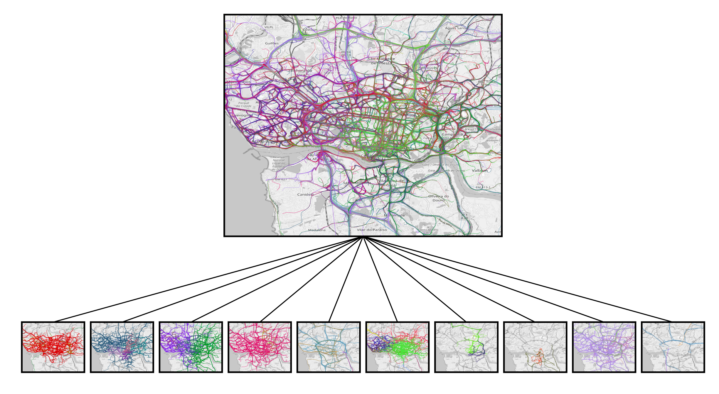
Figure 5: Taxi data. The nested clustering for $10000$ randomly selected trajectories is shown. There are ten non-empty components in the first layer and nine non-empty components in the second layer, corresponding to a GMM with $90$ components shown in the first row. These clusters can be divided into ten subsets (second row) containing up to nine clusters each. The ten subsets are shown in the second row. Note, that many trajectories connect to endpoints outside the shown region. The map was taken from OpenStreetMap.

Even though this hierarchical representation has no very clear interpretation for all clusters, it might be used as a starting point for further exploration. City planners and urban decision makers could be interested in a comparison between start and end points of trajectories in the various clusters to further evaluate the need of connections, for example via public transport, between different regions of the city. Here, the nested structure of the clusters might be helpful, when scanning the clusters for interesting patterns. The $10$ large main clusters based on the first layer give a broad overview, while the sub-clusters allow for a more nuanced analysis. An example is given in Figure 6.

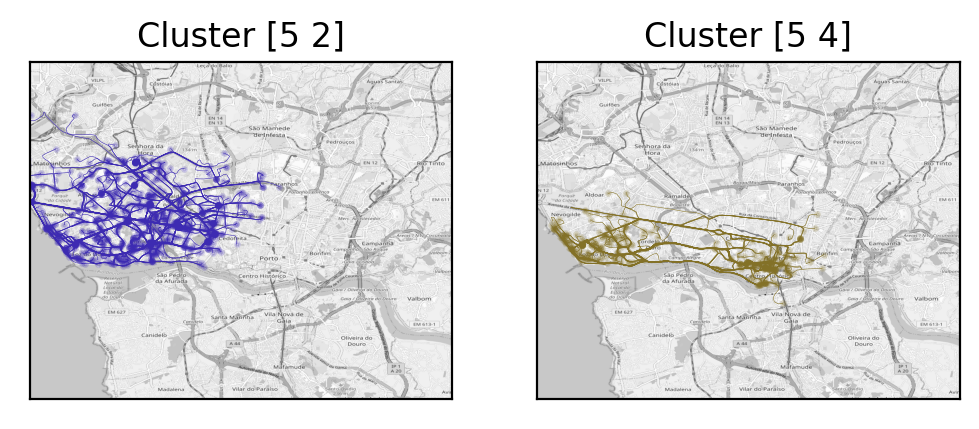
Figure 6: Taxi data. VIdmfa detects two clusters consisting of short trajectories connected to the harbour and seaside. Both clusters belong to the same main cluster $5$. Cluster $[5,2]$ connects to a larger region on the west side of the city outside the center with the taxis passing through smaller streets, while cluster $[5,4]$ connects to the city center. Here the Taxis pass through one of three parallels. The dots denote starting and end points of the trajectories.

7 Conclusion and Discussion

In this paper, we introduced a new method for high-dimensional clustering. The method uses sparsity-inducing priors to regularize the estimation of the DMFA model of Viroli and McLachlan (2019), and uses variational inference methods for computation to achieve scalability to large datasets. We consider the use of overfitted mixtures and ELBO values from short runs to choose a suitable architecture in a computationally thrifty way.

As noted recently by Selosse et al. (2020) deep latent variable models like the DMFA are challenging to fit. It is difficult to estimate large numbers of latent variables, and there are many local modes in the likelihood function. While our sparsity priors are helpful in some cases for obtaining improved clustering and making the estimation more reliable, there is much more work to be done in understanding and robustifying the training of these models. The way that parameters for mixture components at different layers are combined by considering all paths through the network allows a large number of mixture components without a large number of parameters, but this feature may also result in probability mass being put in regions where there is no data. It is also not easy to interpret how the deeper layers of these models assist in explaining variation. A deeper understanding of these issues could lead to further improved architectures and interesting new applications in high-dimensional density estimation and regression.

References

- (1)
- Amari (1998) Amari, S. (1998). Natural gradient works efficiently in learning, Neural Computation 10: 251–276.
- Bartholomew et al. (2011) Bartholomew, D. J., Knott, M. and Moustaki, I. (2011). Latent Variable Models and Factor Analysis: A Unified Approach, 3 edn, John Wiley & Sons.
- Blei et al. (2017) Blei, D. M., Kucukelbir, A. and McAuliffe, J. D. (2017). Variational inference: A review for statisticians, Journal of the American Statistical Association 112(518): 859–877.
- Carvalho et al. (2008) Carvalho, C. M., Chang, J., Lucas, J. E., Nevins, J. R., Wang, Q. and West, M. (2008). High-dimensional sparse factor modeling: Applications in gene expression genomics, Journal of the American Statistical Association 103(484): 1438–1456.
- Carvalho and Polson (2010) Carvalho, C. M. and Polson, Nicholas, G. (2010). The horseshoe estimator for sparse signals, Biometrika 97(2): 465–480.
- Cho et al. (1998) Cho, R. J., Campbell, M. J., Winzeler, E. A., Steinmetz, L., Conway, A., Wodicka, L., Wolfsberg, T. G., Gabrielian, A. E., Landsman, D., Lockhart, D. J. et al. (1998). A genome-wide transcriptional analysis of the mitotic cell cycle, Molecular cell 2(1): 65–73.
- Dayal (2016) Dayal, M. (2016). cepp: Context Driven Exploratory Projection Pursuit. R-package version 1.7.
- Dua and Graff (2017) Dua, D. and Graff, C. (2017). UCI machine learning repository. http://archive.ics.uci.edu/ml.
- Forina et al. (1986) Forina, M., Armanino, C., Castino, M. and Ubigli, M. (1986). Multivariate data analysis as a discriminating method of the origin of wines, Vitis 25(3): 189–201.
- Forina et al. (1983) Forina, M., Armanino, C., Lanteri, S. and Tiscornia, E. (1983). Classification of olive oils from their fatty acid composition, Food research and data analysis: proceedings from the IUFoST Symposium, September 20-23, 1982, Oslo, Norway/edited by H. Martens and H. Russwurm, Jr, London: Applied Science Publishers, 1983.
- Frühwirth-Schnatter and Lopes (2018) Frühwirth-Schnatter, S. and Lopes, H. F. (2018). Sparse Bayesian factor analysis when the number of factors is unknown, arXiv preprint arXiv:1804.04231 .
- Ghahramani and Beal (2000) Ghahramani, Z. and Beal, M. (2000). Variational inference for Bayesian mixtures of factor analysers, in S. Solla, T. Leen and K. Müller (eds), Advances in Neural Information Processing Systems, Vol. 12, MIT Press, pp. 449–455.
- Ghahramani and Hinton (1997) Ghahramani, Z. and Hinton, G. (1997). The EM algorithm for factor analyzers, Technical report, The University of Toronto. https://www.cs.toronto.edu/ hinton/absps/tr-96-1.pdf.
- Hahn et al. (2018) Hahn, P. R., He, J. and Lopes, H. (2018). Bayesian factor model shrinkage for linear IV regression with many instruments, J. of Business & Economic Statistics 36(2): 278–287.
- Hoffman et al. (2013) Hoffman, M. D., Blei, D. M., Wang, C. and Paisley, J. (2013). Stochastic variational inference, Journal of Machine Learning Research 14(1): 1303–1347.
- Honkela et al. (2008) Honkela, A., Tornio, M., Raiko, T. and Karhunen, J. (2008). Natural conjugate gradient in variational inference, in M. Ishikawa, K. Doya, H. Miyamoto and T. Yamakawa (eds), Neural Information Processing, Springer, Berlin, Heidelberg, pp. 305–314.
- Horton and Nakai (1996) Horton, P. and Nakai, K. (1996). A probabilistic classification system for predicting the cellular localization sites of proteins, Proceedings of the Fourth International Conference on Intelligent Systems for Molecular Biology, AAAI Press, pp. 109––115.
- Kucukelbir et al. (2017) Kucukelbir, A., Tran, D., Ranganath, R., Gelman, A. and Blei, D. M. (2017). Automatic differentiation variational inference, Journal of Machine Learning Research 18(1): 430–474.
- Leisch and Dimitriadou (2010) Leisch, F. and Dimitriadou, E. (2010). Machine learning benchmark problems. R-package version 2.1.
- Li (2005) Li, J. (2005). Clustering based on a multilayer mixture model, Journal of Computational and Graphical Statistics 14(3): 547–568.
- Lukashin and Fuchs (2001) Lukashin, A. V. and Fuchs, R. (2001). Analysis of temporal gene expression profiles: Clustering by simulated annealing and determining the optimal number of clusters, Bioinformatics 17(5): 405–414.