Rapid Modification of Neutron Star Surface Magnetic Field: A proposed mechanism for explaining Radio Emission State Changes in Pulsars

Abstract

The radio emission in many pulsars show sudden changes, usually within a period, that cannot be related to the steady state processes within the inner acceleration region (IAR) above the polar cap. These changes are often quasi-periodic in nature, where regular transitions between two or more stable emission states are seen. The durations of these states show a wide variety ranging from several seconds to hours at a time. There are strong, small scale magnetic field structures and huge temperature gradients present at the polar cap surface. We have considered several processes that can cause temporal modifications of the local magnetic field structure and strength at the surface of the polar cap. Using different magnetic field strengths and scales, and also assuming realistic scales of the temperature gradients, the evolutionary timescales of different phenomena affecting the surface magnetic field was estimated. We find that the Hall drift results in faster changes in comparison to both Ohmic decay and thermoelectric effects. A mechanism based on the Partially Screened Gap (PSG) model of the IAR has been proposed, where the Hall and thermoelectric oscillations perturb the polar cap magnetic field to alter the sparking process in the PSG. This is likely to affect the observed radio emission resulting in the observed state changes.

1 Introduction

A rapidly rotating, highly magnetized, neutron star is a unipolar inductor. The region around the star, the magnetosphere, is initially charge starved and can develop extremely high corotation electric fields. In this environment a copious amount of charges from the neutron star as well as those created due to magnetic pair production screens the electric field and form a force-free corotating magnetosphere. At the light cylinder, the magnetic field lines are separated into closed and open field line regions. The charges in the closed field line region corotate with the star, while a relativistic outflow consisting of dense pair plasma is established along the open field line region. The charges flow out of the neutron star in the form of a pulsar wind, and the magnetosphere requires a continuous supply of charges in order to maintain a steady outflow. This supply is generated by pair creation in the magnetosphere which ensures that within a few tens of microseconds the charges are replenished. The coherent radio emission arises due to growth of plasma instabilities in this relativistic outflow in the inner magnetosphere less than 10% of the light cylinder radius (Mitra, 2017). As a result the observer samples the radio emission as a series of narrow single pulses which occupy less that 10% of the pulsar period and each single pulse is highly variable. On the other hand several studies have demonstrated the pulsar profile, formed after averaging several thousand single pulses, to be highly stable (Helfand et al., 1975; Rathnasree & Rankin, 1995). This signifies the extreme stability of the averaging process over timescales of several minutes to hours.

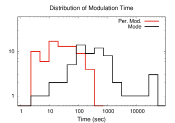
Figure 1: The figure shows the distribution of timescales associated with periodic and quasi-periodic modulations of radio emission from pulsars. The x-axis represents the characteristic times of modulation while the y-axis shows the number of pulsars within each time bin. The periodic modulations (red histogram) consist of periodic nulling and periodic amplitude modulation and are usually seen over a narrow range with periodicities between 10 and 100 seconds. The quasi-periodic variations (black histogram) include emission mode changing as well as the remaining nulling pulsars, and shows a wide range between few tens of seconds to several hours at a time.

Long term monitoring have revealed that in some pulsars the average profile can vary over several different timescales, signifying a change in the emission state (see e.g. Lyne et al., 2010). In most cases such variations are seen in normal long period pulsars, typically having periods longer than 30 milliseconds, although recently similar behaviour has also been reported in young millisecond pulsars (Mahajan et al., 2018). In this paper we will restrict our discussion to normal long period pulsars, and for easy identification we group these variations into Short-Timescale (ST) category, when the timescales of variations last from a single rotation period to a few hours, and Long-Timescale (LT) category, where the variations are observed over months to years (Kramer et al., 2006; Camilo et al., 2012). The LT category include intermittent pulsars, rotating radio transients and normal pulsars (see, e.g., Lyne, 2009; Lyne et al., 2017; Keane & McLaughlin, 2011). The ST category consist of three different phenomena, namely, mode changing, nulling and periodic modulations. Mode changing was first reported in the pulsar B1237+25 by Backer (1970), where the emission switched between two separate states with different but stable profile shapes. The switching between the modes are very rapid and happens within a rotation period, but each mode can last for timescales ranging from minutes to hours. No clear periodic or quasi-periodic behaviour could be associated with mode transitions, although several pulsars have been identified recently, like J1752+2359 (Lewandowski et al., 2004), which exhibit quasi-periodic bursting states. During nulling the emission entirely ceases within a period which lasts over timescales from a single period to several minutes. There are also instances where the pulsar nulls for longer durations lasting hours at a time (Kerr et al., 2014; Naidu et al., 2018). The periodic modulations are further subdivided into periodic amplitude modulations and periodic nulling. In some cases the nulls are found to be periodic and repeats at intervals of several tens to a few hundred periods (Herfindal & Rankin, 2007, 2009; Basu et al., 2017, 2020a). The periodic amplitude modulation is another similar behaviour, where on short time scales of tens to hundreds of periods the pulsar oscillates quasi-periodically between two distinct emission states usually of different intensity levels (Basu et al., 2016; Mitra & Rankin, 2017; Yan et al., 2019, 2020).

A detailed study of periodic modulation in the pulsar population was undertaken in Basu et al. (2020c), that found periodic amplitude modulation to be present in 18 pulsars, while periodic nulling is seen in 29 pulsars. In addition there are another 24 pulsars where periodic modulation is also present, whose nature could not be resolved due to weaker detection sensitivity of the single pulses. The distribution of the modulation periodicity of this population is shown in Fig. 1 (red histogram), where the time has been estimated in seconds. The distribution is restricted to a relatively narrow window between 10-100 seconds. There are around 30-40 pulsars where presence of mode changing have been detected. Table 3 in the appendix presents the details of the timescales associated with the known mode changing pulsars in the literature. The detection of nulling can be confused in weaker pulsars where low intensity single pulses are below detection limit. The presence of unambiguous nulling has been seen in around 80-100 pulsars (Wang et al., 2007; Gajjar et al., 2012; Basu et al., 2020c). Although no underlying periodicity is associated with mode changing and remaining nulling cases, it is still possible to estimate the average durations of the different states. We were able to determine the average timescales associated with nulling and mode changing in around 60 pulsars whose distribution is shown in Fig. 1 (black histogram). Unlike the periodic modulations, these timescales show a much wider variation between few seconds to several hours.

The radio emission only constitute a tiny fraction of the total rotational energy of the neutron star, and hence it is important to understand whether during the state changes there is any detectable change in the slowdown rate of the star. For LT category, it has been shown that the profile changes are accompanied by changes in the spin down rate of the star (Kramer et al., 2006). This opens up the possibility that changes in the global magnetospheric configuration can influence these state changes (Timokhin 2010; Melrose & Yuen 2014). However, in this work we focus on the ST phenomena, where no clear change in the global magnetosphere has been observed during the state changes. Two mode changing pulsars, B0943+10 and B0823+26, have shown synchronous variations in the X-ray emission during radio mode changes (Hermsen et al., 2013, 2018)). Although the X-ray emission carries a higher fraction of the rotational energy compared to the radio emission, during mode transitions, the X-ray emission changes by only a small fraction, around 15%. This is not sufficient to constitute a change in the slowdown energy of the star (Mereghetti & Rigoselli, 2017)). It has also been shown in several cases that in the different modes the radio emission arises from similar locations within the magnetosphere (Brinkman et al., 2019; Rahaman et al., 2021). This further suggests that there is no change in the magnetic field structure or the open field line geometry in the emission region during mode changing. The ST phenomena usually repeat at irregular intervals which also rules out highly periodic processes like precession and/or nutation as possible basis for such changes. Thus it is reasonable to suggest that the ST processes are governed by local changes in the magnetosphere that can effect a change in the radio emission.

Our aim in this work is to highlight a physical mechanism that can explain the ST phenomena in pulsars. Here we consider pulsar radio emission models such as Ruderman & Sutherland (1975); Asseo & Melikidze (1998); Gil et al. (2003); Philippov et al. (2020), where the generation of coherent radio emission is facilitated by nonstationary pair plasma discharges above the pulsar polar cap. This can be best done in the framework of the partially screened gap (PSG, Gil et al., 2003) model, which describes the physics immediately above the polar cap. We suggest that changes in the surface magnetic field on the polar cap over short timescales can bring about changes in the radio emission. We briefly describe below the physical conditions on the polar cap that that can sustain such a mechanism.

1.1 The properties of polar cap influencing coherent radio emission

A widely accepted model for the origin of pair plasma responsible for the coherent radio emission has been proposed by Ruderman & Sutherland (1975), which suggests the existence of an inner acceleration region (IAR) above the polar cap. A system of sparking discharges driven by magnetic pair production is setup in the IAR that supplies a non-stationary flow of relativistic outflowing plasma along the open field line region. Several observational studies suggest that the IAR is dominated by strongly non-dipolar surface magnetic field (e.g. Arumugasamy & Mitra, 2019) and as a consequence is not a pure vacuum gap as was initially assumed by Ruderman & Sutherland (1975), but form a PSG (Gil et al., 2003) due to supply of thermally regulated ions from the stellar surface. The strong non-dipolar nature causes the field lines to become highly curved, thereby enhancing the generation and acceleration of the dense pair plasma in the PSG. The large electric fields in the gap separates the pair plasma in opposite directions. The electrons smash against the polar cap surface and heats it up which causes the iron ions to escape the surface into the gap. The positrons and ions are accelerated outwards by the electric field to relativistic speeds. They produce additional pair cascades which result in a secondary pair plasma flowing outwards along the open field lines. The radio emission is generated in this outflowing plasma due to growth of plasma instabilities (Asseo & Melikidze, 1998; Melikidze et al., 2000; Lakoba et al., 2018; Rahaman et al., 2020).

1.2 The temperature variations on the Neutron star surface

The heated polar cap surface is expected to produce thermal X-ray emission which can in turn be used to find its area and temperature. Studies of time-aligned radio and thermal X-ray emission reveal that the polar cap region is dominated by strong small scale field and hence is smaller than what is expected from a purely dipolar configuration (Geppert et al., 2013; Szary et al., 2017). Further the polar cap temperatures have been measured to exceed $3\times 10^{6}$ K. It has also been shown that a large temperature difference exist between the polar cap and the rest of the neutron star surface. This results in enormous temperature gradients both in radial and meridional directions between the polar cap envelope and the surrounding regions, which are restricted to within a very shallow layer beneath the surface. The kinetic energy of the backflowing charges is released as heat within a few radiation lengths and is immediately re-radiated, without practically any thermal energy being transported deeper into the crust (Cheng & Ruderman, 1980; Sznajder & Geppert, 2020). The lifetime of radio pulsars are typically around $10^{6}$ to $10^{7}$ years, during which the polar cap area remains significantly hotter than the remaining surface. Since the magnetic field penetrating the polar cap surface is dominated by strong radial components, very effective thermal insulation is present at the rim of the polar cap. The remaining surface cools in accordance with quite well understood processes (URCA or DURCA, photons), thereby increasing the meridional temperature gradient with time. After $\sim 10^{6}$ years the remaining surface has temperatures around few times $10^{5}$ K (Page et al., 2006; Viganò et al., 2013).

1.3 Magnetic field variations at small spatial scales on the Neutron star surface

The magnetic field at the polar cap is maintained by small scale currents circulating beneath its surface. These currents are generated and maintained by the continuous transfer of magnetic flux from a large scale toroidal field reservoir into small scale poloidal structures via the Hall drift (Reisenegger et al., 2007; Geppert & Viganò, 2014). The formation of such magnetic spots has been recently demonstrated in 3-dimensional simulations by Gourgouliatos & Hollerbach (2018). The magnetic spots are confined to small spatial regions, and extreme thermal insulation of the polar cap by the strong local poloidal field ensure that the magnetic field variations in these small regions are independent of the global magneto-thermal evolution of the neutron star.

In this paper we suggest that the Hall drift and thermoelectrically driven magnetic field oscillations at the polar cap surface is a possible explanation for the observed ST phenomena in pulsars. Estimates of the timescales associated with these processes have been carried out which match the observations. We also present a mechanism where these changes in the surface field affect the sparking process in the polar cap thereby inducing changes in the pulsar radio emission in a quasi-periodic manner. In section 2 we give the framework for the variations in the magnetic field and estimate the timescales involved. In section 3 and  4 we propose a model for the ST phenomena and present our conclusions.

2 Timescale Analysis of magnetic field variation over polar cap

2.1 Basic equations

The surface of the polar cap is made up of highly conducting iron nuclei that are either in a liquified or crystallized state. A striking feature of this region is the presence of extremely large temperature gradients; especially in radial direction as well as the meridional direction. The magnetic field evolution is governed by the induction equation :

$$\frac{\partial\vec{B}}{\partial t}=-c\vec{\nabla}\times\vec{E}\;,$$ (1)

where the electric field $\vec{E}$ is given by Ohm’s law and is a sum of three terms:

$$\vec{E}=\frac{c}{4\pi\hat{\sigma}}\vec{\nabla}\times\vec{B}-\frac{\vec{v}_{adv}}{c}\times\vec{B}-\vec{E}^{ext}\;.$$ (2)

The first term contains the tensor of the electric conductivity $\hat{\sigma}$. The components of $\hat{\sigma}$ that are perpendicular to the direction of the magnetic field are responsible for the Hall drift of the magnetic field. The first term also contains the effect of the usual Ohmic diffusion. The second term in Eq. 2 is the advection term where $\vec{v}_{adv}$ is the advection velocity and this term is relevant only when the matter at the polar cap is in a liquified state, which is possible when the temperatures are extremely high. Such a situation is unlikely to be realized in radio pulsars considered here (see Sect. 2.2). The nature of the external electric field $\vec{E}^{ext}$, which constitute the third term, is determined by the presence of huge temperature gradients. These gradients are especially strong in the radial direction where they can exceed $\sim 10^{8}$ Kcm^-1. Across the rim of the polar cap the meridional temperature gradients of $\sim 10^{4}$ Kcm^-1 may drive a thermoelectric instability which causes the generation of an azimuthal magnetic field along that rim (Blandford et al., 1983; Urpin et al., 1986; Geppert & Wiebicke, 1995). In the context of emission mode changing the thermal drift of the magnetic field by these temperature gradients are of special interest. It may cause an oscillating behaviour of the local magnetic field structures at the real polar cap surface.

If at the polar cap $\vec{v}_{adv}=0$, the two remaining electric field constituents in Eq. 2 have the following form:

$$\frac{c^{2}}{4\pi\hat{\sigma}}\vec{\nabla}\times\vec{B}=\eta_{B}\vec{\nabla}\times\vec{B}+\alpha_{H}(\vec{\nabla}\times\vec{B})\times\vec{B}$$

$$\eta_{B}=\frac{c^{2}}{4\pi\sigma}\;,\;\;\alpha_{H}=\eta_{B}\frac{\omega_{B}\tau}{B}\;,$$ (3)

where $\sigma$ is the electric conductivity tensor component parallel to $\vec{B}$, $\omega_{B}\tau$ the magnetization parameter, and $B$ the magnitude of the magnetic field vector $\vec{B}$. The thermoelectric field is given as:

$$\vec{E}^{ext}=\vec{E}_{T} = -Q(3+\xi)\vec{\nabla}T$$ (4)

$$+ \frac{Q\xi\omega_{B}\tau}{1+\omega_{B}^{2}\tau^{2}}\left[\vec{\nabla}T+\omega_{B}\tau(\vec{b}\times\vec{\nabla}T)\right]\times\vec{b}\;.$$

In these equations $\vec{b}$ is the unit vector along $\vec{B}$ and $\omega_{B}\tau$ is the magnetization parameter, indicating the strength of magnetization of the electron plasma. The magnetic diffusivity $\eta_{B}$ depends on $\sigma$. The thermopower $Q$, the coefficient $\xi$, as well as the derivation of Eq. 4 are explained in detail in the Appendix 5.5. The first term in the r.h.s. of Eq. 4 describes the thermoelectric battery. If the coefficient $Q(3+\xi)$ depends on the radial coordinate $r$ and a meridional temperature gradient $dT/rd\theta$ is present, this effect may amplify an azimuthal seed field. For the study of local magnetic field oscillations the second term is of interest. It can be interpreted, similar to the Hall drift, as the thermal drift of the magnetic field with the thermal drift velocity, $\vec{v}_{TD}/c\times\vec{B}$, where

$$\vec{v}_{TD}=\frac{Q\xi e\tau}{m_{\ast}(1+\omega_{B}^{2}\tau^{2})}\left[\vec{\nabla}T+\omega_{B}\tau(\vec{b}\times\vec{\nabla}T)\right]\;.$$ (5)

In the limit $\omega_{B}\tau\gg 1$, which is expected to be valid in the polar cap region of radio pulsars, $\vec{E}_{T}$ simplifies to

$$\vec{E}_{T}=-Q(3+\xi)\vec{\nabla}T+Q\xi(\vec{b}\times\vec{\nabla}T)\times\vec{b}.$$ (6)

The $\mathrm{curl}$ of Eqs. 3 and 6 leave us with the induction equations govern the magnetic field evolution by Ohmic diffusion, the Hall drift, and thermoelectric effects.

The magneto-thermal evolution at the polar cap surface is a complex non-linear process whose detailed interpretation can be obtained only from numerical modelling. However, in order to get a basic idea of the processes from analytical results we will use the following simplifications:

1. Axial symmetry is assumed. This greatly simplifies the use of poloidal - toroidal representation of the magnetic field: $\vec{B}=\vec{B}_{p}+\vec{B}_{t}$. Under this assumption the poloidal and toroidal components of $\vec{B}$ have the following properties:

   1. $\vec{\nabla}\times\vec{B}_{p}$ is toroidal, $\vec{\nabla}\times\vec{B}_{t}$ is poloidal,

   2. $\vec{B}_{p}\cdot\vec{B}_{t}=0$,

   3. $\vec{B}_{p}\times\vec{B}_{t}$ is poloidal,

   4. $\vec{B}_{p}\times\vec{B}_{p}=0$,

   5. $\vec{B}_{t}\times\vec{B}_{t}=0$.

2. The magnetic field evolution at the polar cap surface take place within a very thin layer. Therefore, we will consider all transport coefficients as independent of coordinates.

Without the above simplifications one would require much less illustrative dispersion relations to describe the physical behaviour. But it is unclear whether any essential physics is neglected by using these assumptions.

As shown below, the advective term in Eq. 2 can be neglected in our analysis. The remaining constituents of the elcetric field $\vec{E}$ in Eq.  1, given by Eq.  3 and Eq.  4 will cause different temporal variations of the magnetic field $\vec{B}$. One would expect that the Hall induction equation, related to the tensor of the electric conductivity describes a faster magnetic field variation than the thermoelectric induction equation related to $\vec{E}_{T}$. Under the above given simplifications, the Hall induction equation is given as:

$$\left(\frac{\partial\vec{B}}{\partial t}\right)_{Ohm,Hall}=-\eta_{B}\vec{\nabla}\times\left[\vec{\nabla}\times\vec{B}\right]+\alpha_{H}\vec{\nabla}\times\left[(\vec{\nabla}\times\vec{B})\times\vec{B}\right]\;,$$ (7)

while the effect of temperature gradients on the magnetic field evolution is of the form:

$$\left(\frac{\partial\vec{B}}{\partial t}\right)_{TE}=-\vec{\nabla}\times\left[\alpha_{T}\vec{\nabla}T-\beta_{T}\left(\vec{B}\times\vec{\nabla}T\right)\times\vec{B}\right]\;,$$ (8)

where $\alpha_{T}=cQ(3+\xi)$ and $\beta_{T}=cQ\xi/B^{2}$. The first term in the r.h.s. of Eq.  8 describes effect of thermoelectric battery. It is independent of $\vec{B}$ and could contribute only to a toroidal seed field. Since $\vec{\nabla}\times\left(\alpha_{T}\vec{\nabla}T\right)=\vec{\nabla}\alpha_{T}\times\vec{\nabla}T$, this term vanishes in our approximation of coordinate independent transport coefficients. Thus, in this study we will calculate the dispersion relations of magnetic perturbations, whose evolution is determined by Eqs. 7 and 8. But before that we will discus the physical conditions at the polar cap.

2.2 Conditions of aggregation at the polar cap surface

An important issue relevant to this work is the surface density at the hot polar cap, where the neutron star matter is condensed, either in liquified or solidified state. The most recent description of the state of aggregation in this region is provided in Potekhin & Chabrier (2013). The so called zero pressure density can be considered at the surface which is bombarded with ultra-relativistic electrons. It increases with the local magnetic field strength, $\propto B_{12}^{6/5}$, and is estimated as:

$$\rho_{s}=561\zeta AZ^{-3/5}B_{12}^{6/5}\,\,,\zeta\approx 0.517+0.24B_{12}^{1/5}\,,$$ (9)

where $B_{12}=B/10^{12}$G. In case of a surface made up of Fe ($A=56,Z=26$), $\rho_{s}\approx 5.1\times 10^{5},1.25\times 10^{6},...$ g cm^-3 for local field strengths $B_{12}=50,100,...$, respectively, as expected at the non-dipolar polar cap surface. The Coulomb coupling parameter, $\Gamma_{m}(B)$, which depends on the magnetic field, determines the state of surface matter, i.e., whether it is liquid or solid. If $\Gamma_{m}(B)>175$ the matter is in a solidified form, while below this value it is a liquid. The parameter is estimated in Potekhin & Chabrier (2013) as:

$$\Gamma_{m}(B)\approx\Gamma(0)\left[1+0.2\beta\right]^{-1}\,.$$ (10)

Here $\beta$ is given by the ratio of ion cyclotron to ion plasma frequency, $\beta\approx 0.0094B_{12}\rho_{6}^{-1/2}$ with $\rho_{6}=\rho/10^{6}$ gcm^-3. $\Gamma(0)$ is roughly the ratio of Coulomb and thermal energies,

$$\Gamma(0)=\frac{(Ze)^{2}}{a_{i}k_{B}T}\approx\frac{22.747}{T_{6}}\rho_{6}Z^{2}A^{-1/3}\,,$$ (11)

with $a_{i}$ being the spacing between ions and $k_{B}$ is the Boltzmann constant. Inserting typical values for the surface temperature at the polar cap, $T_{6}\approx 3,5$ (see e.g. Szary et al., 2017) and $\rho_{6}\approx 0.51,1.25$, one finds $\Gamma_{m}\approx 974,1235$ if $T_{6}=3$ and $\Gamma_{m}\approx 400,1000$ if $T_{6}=5$ for $B_{12}=50,100$, respectively. In all cases $\Gamma_{m}(B)$ is significantly larger then $175$. Hence, the polar cap surface of radio pulsars is in a solidified state. For this reason an advection of the polar cap magnetic field is impossible and the corresponding term $\nabla\times(\frac{\vec{v}_{adv}}{c}\times\vec{B})$ in Eq. 2 can be safely neglected.

2.3 Local magnetic field structure at the polar cap surface

An useful approximation for the non-dipolar magnetic field on the polar cap surface has been suggested by Gil et al. (2002), who consider the field to be a superposition of a star centered global dipole and a crust anchored surface dipole, $\vec{B}_{s}=\vec{B}_{d}+\vec{B}_{p}$. The magnetic field near the polar cap is dominated by the surface dipole, while at large distances from the star the global dipole takes precedence. In this configuration the magnetic field structure near the surface differs greatly from a purely dipolar one, but the field lines reconnects with the dipolar field at altitudes of about few hundred meters. We have used the surface dipole to be characterized as $\vec{B}_{p}=B_{p0}\frac{R_{pc}^{3}}{r^{3}}\left(\mathrm{cos}\theta\hat{e}_{r}+\frac{1}{2}\mathrm{sin}\theta\hat{e}_{\theta}\right)$, where $R_{pc}$ is the dipolar polar cap radius. The global dipole has typical strength of a few times $10^{12}$ G at the polar cap surface. The local dipole is expected to be located at a depth of $\sim 5\times 10^{3}$ cm below the crust, which is approximately the size of the non-dipolar polar cap radius $R_{pc}$ (see Table 1 in Geppert, 2017). Using $rd\theta\approx 5\times 10^{3}$ cm, the meridional angle directed from the pole of $\vec{B}_{p0}$ to the rim of the polar cap is $\theta\approx 45^{\circ}$.

2.4 Hall oscillations

We follow the method presented in Shalybkov & Urpin (1997) to derive the dispersion relation for coupled Ohmic decay and Hall drift. In the presence of strong magnetic fields the electric conductivity becomes a tensor. The decomposition of the magnetic field into poloidal and toroidal components transforms the induction Eq. 7 into coupled differential equations of the form:

$$\frac{\partial\vec{B}_{p}}{\partial t} = -\eta_{B}\left[\vec{\nabla}\times(\vec{\nabla}\times\vec{B}_{p})\right]$$ (12)

$$- \alpha_{H}\vec{\nabla}\times\left[(\vec{\nabla}\times\vec{B}_{t})\times\vec{B}_{p}\right]\;,\;$$

$$\frac{\partial\vec{B}_{t}}{\partial t} = -\eta_{B}\left[\vec{\nabla}\times(\vec{\nabla}\times\vec{B}_{t})\right]$$ (13)

$$- \alpha_{H}\vec{\nabla}\times\left[(\vec{\nabla}\times\vec{B}_{p})\times\vec{B}_{p}+(\vec{\nabla}\times\vec{B}_{t})\times\vec{B}_{t}\right]\;.$$

We introduce small perturbations $\delta\vec{B}_{p},\delta\vec{B}_{t}$, to the background magnetic field components $\vec{B}_{p0},\vec{B}_{t0}$, similar to Shalybkov & Urpin (1997), such that $\vec{B}_{p}=\vec{B}_{p0}+\delta\vec{B}_{p}$ and $\vec{B}_{t}=\delta\vec{B}_{t}$ ($\vec{B}_{t0}=0$ is assumed). The Hall-Induction equations up to first order in the perturbations are obtained as:

$$\frac{\partial\delta\vec{B}_{p}}{\partial t}=-\eta_{B}\left[\vec{\nabla}\times(\vec{\nabla}\times\delta\vec{B}_{p})\right]-\alpha_{H}\vec{\nabla}\times\left[(\vec{\nabla}\times\delta\vec{B}_{t})\times\vec{B}_{p0}\right]\;,$$ (14)

$$\frac{\partial\delta\vec{B}_{t}}{\partial t}=-\eta_{B}\left[\vec{\nabla}\times(\vec{\nabla}\times\delta\vec{B}_{t})\right]-\alpha_{H}\vec{\nabla}\times\left[(\vec{\nabla}\times\delta\vec{B}_{p})\times\vec{B}_{p0}\right]\;,$$ (15)

The differential equations are transformed into algebraic ones by using Fourier transformation. The process is described in Appendix 5.3 for the Ohmic decay terms in Eqs. 14 and 15. If we consider the Hall term for poloidal perturbation in Eq.14 which is of the form

$$-\alpha_{H}\vec{\nabla}\times\left[(\vec{\nabla}\times\delta\vec{B}_{t})\times\vec{B}_{p0}\right]\;,$$ (16)

the corresponding expression in Eq. 12 is $\alpha_{H}(\vec{k}\vec{B}_{p0})\times\delta\vec{B}_{t}$. Applying the same procedure to the Hall term of Eq. 13 we get $\alpha_{H}(\vec{k}\vec{B}_{p0})\times\delta\vec{B}_{p}$. This leads to a set of two algebraic equations

$$\left(i\omega+\eta_{B}k^{2}\right)\delta\vec{B}_{p}=-\alpha_{H}(\vec{k}\cdot\vec{B}_{p0})\vec{k}\times\delta\vec{B}_{t}\;,$$ (17)

$$\left(i\omega+\eta_{B}k^{2}\right)\delta\vec{B}_{t}=-\alpha_{H}(\vec{k}\cdot\vec{B}_{p0})\vec{k}\times\delta\vec{B}_{p}\;.$$ (18)

This system of equations can be easily solved by substituting

$$\delta\vec{B}_{t}=-\alpha_{H}\frac{(\vec{k}\cdot\vec{B}_{p0})\vec{k}}{(i\omega+\eta_{B}k^{2})}\times\delta\vec{B}_{p}\,,$$ (19)

to find the dispersion relation for both the toroidal and poloidal perturbation as

$$\omega_{\pm}=i\eta_{B}k^{2}\pm\alpha_{H}(\vec{k}\cdot\vec{B}_{p0})k=i\eta_{B}k^{2}\pm\omega_{Hall}\,.$$ (20)

The first term in the r.h.s. of Eq.  20 describes the (perhaps slow) Ohmic decay of the Hall wave amplitudes, while the second term is the frequency of the sinusoidal Hall waves, sometimes called helicoidal or Whistler waves. As pointed out in Shalybkov & Urpin (1997), this Hall waves may appear in strong magnetic fields, $\vec{k}\cdot\vec{B}_{p0}\gg 1$, with relatively small wavelengths, which is applicable for the polar cap of radio pulsars.

2.5 Thermal drift oscillations

In the limit $\omega_{B}\tau\gg 1$ the thermal electric field, $\vec{E}_{T}$, simplifies to the form (see Appendix 5.5, Eq. 53 and 55)

$$\vec{E}_{T}=-Q(3+\xi)\vec{\nabla}T+Q\xi(\vec{b}\times\vec{\nabla}T)\times\vec{b}.$$ (21)

The curl of $\vec{E}_{T}$ gives the ‘thermal’ induction equation

$$\frac{\partial\vec{B}}{\partial t}=-\vec{\nabla}\times\left[\alpha_{T}\vec{\nabla}T-\beta_{T}\left(\vec{B}\times\vec{\nabla}T\right)\times\vec{B}\right]\;.$$ (22)

where $\alpha_{T}=cQ(3+\xi)$ and $\beta_{T}=cQ\xi/B^{2}$. The first term in the r.h.s. of Eq.  22 is the thermoelectric battery term. It is independent of $\vec{B}$ and can only contribute to the toroidal background field $\vec{B}_{t0}$. Since $\vec{\nabla}\times\left(\alpha_{T}\vec{\nabla}T\right)=\vec{\nabla}\alpha_{T}\times\vec{\nabla}T$, this term vanishes in our approximation of coordinate independent transport coefficients, and only the remaining term in the r.h.s. of Eq.  22 describes the thermal drift of magnetic field. The drift velocity $\vec{v}_{TD}=\beta_{T}\left(\vec{B}\times\vec{\nabla}T\right)$ depends on the magnetic field and can affect the field evolution in the presence of strong temperature gradients, which are typically present both in radial and in meridional direction of the polar cap surface.

Assuming $\beta_{T}$ to be independent of coordinates, and applying the decomposition of the magnetic field into poloidal and toroidal components we have

$$\frac{\partial\vec{B}}{\partial t} = -\beta_{T}\vec{\nabla}\times\left[(\vec{B}_{p}\times\vec{\nabla}T)\times\vec{B}_{p}\right]$$ (23)

$$- \beta_{T}\vec{\nabla}\times\left[(\vec{B}_{t}\times\vec{\nabla}T)\times\vec{B}_{p}\right]$$

$$- \beta_{T}\vec{\nabla}\times\left[(\vec{B}_{t}\times\vec{\nabla}T)\times\vec{B}_{t}\right]\;.$$

The first and third terms in Eq. 23 are toroidal fields while the second term is poloidal in nature. Thus, the thermal drift $\sim\vec{\nabla}T$ acts directly on both $\vec{B}_{t}$ and $\vec{B}_{p}$. Following the same procedure as above for the dispersion relation of Hall waves, the induction equations till first order in $\delta\vec{B}_{p,t}$ are given as:

$$\frac{\partial\delta\vec{B}_{p}}{\partial t}=-\beta_{T}\vec{\nabla}\times\left[(\delta\vec{B}_{t}\times T^{\prime})\times\vec{B}_{p0}\right]\;,$$ (24)

$$\frac{\partial\delta\vec{B}_{t}}{\partial t}=-\beta_{T}\vec{\nabla}\times\left[(\delta\vec{B}_{p}\times T^{\prime})\times\vec{B}_{p0}+(\vec{B}_{p0}\times T^{\prime})\times\delta\vec{B}_{p}\right]\;,$$ (25)

where $T^{\prime}$ denotes $\vec{\nabla}T$, a quantity which is assumed to be unperturbed over timescales of magnetic field variations. We first consider the evolution of the poloidal component of the magnetic field perturbation because it may affect the emission regime above the polar cap surface:

$$\frac{\partial\delta\vec{B}_{p}}{\partial t} = \beta_{T}\vec{\nabla}\times\left[\vec{B}_{p0}\times(\delta\vec{B}_{t}\times T^{\prime})\right]$$ (26)

$$= \beta_{T}\vec{\nabla}\times\left[\delta\vec{B}_{t}(\vec{B}_{p0}\cdot T^{\prime})-T^{\prime}(\vec{B}_{p0}\cdot\delta\vec{B}_{t})\right]\;.$$

The last term $\vec{B}_{p0}\cdot\delta\vec{B}_{t}$ vanishes because in axial symmetry the scalar product of a poloidal and a toroidal vector is zero. The curl of the remaining equation gives

$$\frac{\partial\delta\vec{B}_{p}}{\partial t}=\beta_{T}\left[(\vec{B}_{p0}\cdot T^{\prime})\vec{\nabla}\times\delta\vec{B}_{t}+\vec{\nabla}(\vec{B}_{p0}\cdot T^{\prime})\times\delta\vec{B}_{t}\right]\;.$$ (27)

We have used the abbreviation $m=(\vec{B}_{p0}\cdot T^{\prime})$. Fourier transformations on the above equation gives us the relation

$$i\omega\delta\vec{B}_{p}=\beta_{T}(m^{\prime}-im\vec{k})\times\delta\vec{B}_{t}\;.$$ (28)

In order to solve this equation we couple the poloidal perturbation caused by $\vec{v}_{TD}$ to the toroidal perturbation caused by the Hall drift, i.e. we couple the thermal drift oscillations to the rapidly varying Hall drift oscillations. If $\delta\vec{B}_{t}$ is replaced by the expression in Eq. 19,

$$\delta\vec{B}_{t}=-\frac{n}{(i\omega+\eta_{B}k^{2})}\vec{k}\times\delta\vec{B}_{p}\;$$ (29)

where $n=\alpha_{H}(\vec{k}\cdot\vec{B}_{p0})$, into Eq.  28 and rearranging the vector product we obtain

$$i\omega(i\omega+\eta_{B}k^{2})\delta\vec{B}_{p} = n\beta_{T}\left[(m^{\prime}-im\vec{k})\times\delta\vec{B}_{p}\right]\times\vec{k}$$ (30)

$$= n\beta_{T}\left[(m^{\prime}-im\vec{k})\cdot\vec{k}\right]\delta\vec{B}_{p}\;,$$

as in plane waves $\delta\vec{B}_{p}\cdot\vec{k}=0$ and we assume $m^{\prime}\parallel\vec{k}$ . Solving the above quadratic equation gives

$$\omega_{\pm}=i\frac{\eta_{B}k^{2}}{2}\pm\sqrt{-\frac{\eta_{B}^{2}k^{4}}{4}-n\beta_{T}m^{\prime}\cdot\vec{k}+in\beta_{T}mk^{2}}\;.$$ (31)

The real part of $\omega_{\pm}$ describes the frequency of the thermal drift oscillations of the poloidal magnetic field component. The real part of $\omega_{\pm}$ has the form (see Appendix 5.6)

$$\omega_{+}\approx\frac{\eta_{B}k^{2}}{2}\sqrt{\frac{4n\beta_{T}(m^{\prime}\cdot\vec{k})}{\eta_{B}^{2}k^{4}}+1}\;.$$ (32)

We have termed the scalar product of the background poloidal magnetic field and the temperature gradient, $m=(\vec{B}_{p0}\cdot T^{\prime})$, as ‘magnetic temperature gradient’. This quantity is always negative at the polar cap surface, because the temperature within the polar cap decreases both with increasing radial and meridional coordinates, $dr$ and $rd\theta$. In the following analysis we use spherical coordinates related to the center of the local dipole (see Sec. 2.3). Assuming $m^{\prime}\parallel\vec{k}$ we have to first study $m^{\prime}=\vec{\nabla}(\vec{\nabla}T\cdot\vec{B}_{p0})$. Clearly, $m^{\prime}$ contains first derivatives of the magnetic field components as well as the first and second derivatives of temperature along the radial and meridional coordinates. We evaluate $m^{\prime}$ in spherical coordinates using axial symmetry, and for simplicity replace $\vec{B}_{p0}$ with $\vec{B}$

$$\vec{\nabla}T\cdot\vec{B} = \left(\frac{\partial T}{\partial r}\hat{e}_{r}+\frac{1}{r}\frac{\partial T}{\partial\theta}\hat{e}_{\theta}\right)\cdot(B_{r}\hat{e}_{r}+B_{\theta}\hat{e}_{\theta})$$ (33)

$$= B_{r}\frac{\partial T}{\partial r}+\frac{\frac{\partial T}{\partial\theta}}{r}\frac{\partial T}{\partial\theta}\;.$$

From $\vec{\nabla}(\vec{\nabla}T\cdot\vec{B})=(\vec{\nabla}T\cdot\vec{\nabla})\vec{B}+(\vec{B}\cdot\vec{\nabla})\vec{\nabla}T+\vec{\nabla}T\times(\vec{\nabla}\times\vec{B})\;,(\vec{B}\times(\vec{\nabla}\times(\vec{\nabla}T)))=0$ because $\vec{\nabla}\times(\vec{\nabla}T)=0$, we find for the $r$-component of $m^{\prime}=\vec{\nabla}(\vec{\nabla}T\cdot\vec{B})$:

$$\frac{1}{r^{2}}\frac{\partial T}{\partial\theta}B_{\theta}+\frac{1}{r}\frac{\partial T}{\partial\theta}\frac{\partial B_{\theta}}{\partial r}+\frac{\partial T}{\partial r}\frac{\partial B_{r}}{\partial r}$$

$$+B_{r}\frac{\partial^{2}T}{\partial r^{2}}+\frac{B_{\theta}}{r}\frac{\partial^{2}T}{\partial r\partial\theta}\;,$$ (34)

and for the $\theta$-component of $m^{\prime}=\vec{\nabla}(\vec{\nabla}T\cdot\vec{B})$:

$$-\frac{1}{r}\frac{\partial T}{\partial r}B_{\theta}+\frac{1}{r}\frac{\partial T}{\partial r}\frac{\partial B_{r}}{\partial\theta}+\frac{1}{r^{2}}\frac{\partial T}{\partial\theta}\frac{\partial B_{\theta}}{\partial\theta}$$

$$+\frac{B_{r}}{r}\frac{\partial^{2}T}{\partial r\partial\theta}-\frac{B_{r}}{r^{2}}\frac{\partial T}{\partial\theta}+\frac{B_{\theta}}{r^{2}}\frac{\partial^{2}T}{\partial\theta^{2}}\;.$$ (35)

Using specifications of the local dipole field at the surface as $r=R_{pc}=5\times 10^{3}$ cm, $\vec{B}_{p0}=B_{p0}(\mathrm{cos}{\theta}\hat{e}_{r}+\frac{1}{2}\mathrm{sin}{\theta}\hat{e}_{\theta})$, the derivatives of the magnetic field appearing in Eqs. 34 and 35 are

$$\frac{\partial B_{r}}{\partial r} = -3B_{p0}\frac{R_{pc}^{3}}{r^{4}}(\mathrm{cos}{\theta})\;,$$

$$\frac{\partial B_{\theta}}{\partial r} = -3B_{p0}\frac{R_{pc}^{3}}{2r^{4}}(\mathrm{sin}{\theta})\;,$$

$$\frac{\partial B_{r}}{\partial\theta} = -B_{p0}\frac{R_{pc}^{3}}{r^{3}}(\mathrm{sin}{\theta})\;,$$

$$\frac{\partial B_{\theta}}{\partial\theta} = B_{p0}\frac{R_{pc}^{3}}{2r^{3}}(\mathrm{cos}{\theta})\;.$$ (36)

Note that at the rim of the polar cap, $R_{pc}$, $\theta\sim 45^{\circ}$. Clearly, at $r=R_{pc}$ and in the vicinity of the magnetic pole $\frac{\partial B_{r}}{\partial\theta}$ is the largest partial derivative of the background magnetic field. For the primary contributions to $m^{\prime}$ we find from the first two terms of the $\theta$ component of $m^{\prime}$ (see Eq. 35)

$$m^{\prime}\approx-\frac{3}{2}\frac{1}{r}\frac{\partial T}{\partial r}B_{p0}\mathrm{sin}{\theta}\hat{e}_{\theta}\;.$$ (37)

We can further estimate the partial derivatives of the surface temperature at the polar cap. For the radial derivative $\frac{\partial T}{\partial r}$ we use the fact that all the heat flux arriving at the surface is radiated away as blackbody radiation.

$$\frac{\partial T}{\partial r}=-\frac{1}{\kappa}\sigma_{SB}T_{s}^{4}\;,$$ (38)

where $\sigma_{SB}$ is the Stefan-Boltzmann constant and $\kappa$ is the heat conductivity. For $\kappa\approx 5\times 10^{13}$ erg s^-1 cm^-1 K^-1 and $T=5\times 10^{6}$ K, this results in $\frac{\partial T}{\partial r}\approx 7\times 10^{8}$ K cm^-1. The meridional temperature gradient at the polar cap surface $\frac{\partial T}{R\partial\theta}$ corresponds to a drop of the temperature by a few $10^{6}$ K over the rim of the polar cap, i.e. over a distance of a few $10$ to about $100$ m. Therefore, $\frac{\partial T}{R\partial\theta}\gtrsim 10^{4}$ K cm^-1. Hence, the radial term dominates the partial derivative of the surface temperature gradient. Also, in Eq. 34 and 35, the second derivatives of the temperature can be safely neglected since they are much smaller than the first derivatives. Using these arguments we find

$$m^{\prime}=\vec{\nabla}(\vec{\nabla}T\cdot\vec{B})=\frac{3B_{p0}\sigma_{SB}T_{s}^{4}}{2\kappa R_{pc}}\mathrm{sin}{\theta}\vec{e}_{\theta}\;.$$ (39)

at the surface of the polar cap. Inserting the abbreviations we find the thermal drift oscillation frequency of the magnetic field perturbations as

$$\omega_{TD}=\frac{\eta_{B}k^{2}}{2}\sqrt{\frac{6\omega_{B}\tau cQ\xi\sigma_{SB}T_{s}^{4}}{B_{p0}\kappa R_{pc}\eta_{B}k^{2}}\mathrm{sin}{\theta}+1}\;.$$ (40)

2.6 Rough estimates

In order to get an idea of the magnitude of Hall and thermal magnetic field oscillations we consider the conditions at the polar cap surface with the local dipolar poloidal background magnetic field. We consider two different field strengths $B_{p0}=10^{14}$ G and $B_{p0}=5\times 10^{13}$ G, covering roughly the range of inferred field strengths of polar caps (see Table 1 in Geppert, 2017). These field strengths imply that for Iron nuclei the zero pressure densities are $\rho_{s}=1.25\times 10^{6}$ and $5.1\times 10^{5}$ g cm^-3, respectively. We assume a surface temperature $T=T_{s}=5\times 10^{6}$ K. Using these values the electron number density $n_{e}$, the Fermi momentum $p_{F}$, and the effective electron mass $m_{\ast}$ are:

$$n_{e}=\frac{\rho Z}{Am_{u}}\;,p_{F}=\hbar(3\pi^{2}n_{e})^{1/3}\;,m_{\ast}=c^{-2}(m_{e}^{2}c^{4}+c^{2}p_{F}^{2})^{1/2}\;$$ (41)

To determine the coefficient $\xi$ we follow Urpin & Yakovlev (1980). As the condition $\Theta_{D}/4<T<T_{melt}$ is clearly valid for surface temperatures $T\gtrsim 3\times 10^{6}$ K ($\Theta_{D}$ and $T_{melt}$ are the Debye and melting temperature of the crystalline crust, respectively), this can be used to obtain:

$$\xi=\frac{2-3\beta^{2}}{2+\beta^{2}},\;\beta=\frac{v_{F}}{c},\;v_{F}=\frac{p_{F}}{m_{\ast}}\;.$$ (42)

The transport coefficients depend on the strong background field $B_{p0}$. Both the perpendicular and ‘Hall’ to $\vec{B}_{p0}$ components of the electric conductivity $\hat{\sigma}$, the heat conductivity $\hat{\kappa}$, and the ‘Hall’ component of the thermopower $\hat{Q}$ are drastically reduced by a factor $(\omega_{B}\tau)^{2}$. In case of the Hall drift induced oscillations this effect is automatically taken into account because the Hall-term in Eq. 7 arises from the tensor properties of $\hat{\sigma}$. The same is true for the thermal drift term in Eq. 21. The heat flux, however, dominates parallel to $\vec{B}_{p0}$ in the polar cap region, so that $\kappa$ appearing in Eq. 38 is weakly dependent on the local magnetic field. Therefore, we have used the scalar values of the transport coefficients that are parallel to $\vec{B}_{p0}$. The conductivities decrease with increasing field strength for constant density. In the density and temperature ranges under consideration, magnetic fields stronger than $\sim 10^{12}$G quantize, resulting in Shubnikov - de Haas oscillations of the conductivities (Schubnikow & de Haas, 1930). The (transport-) coefficients were calculated using publicly available codes provided by Potekhin et al. (see http://www.ioffe.ru/astro/EIP/index.html and http://www.ioffe.ru/astro/conduct). For the given density, temperature, and using Iron nuclei as constituent of the polar cap surface the estimated transport coefficients are shown in Tab. 1 (the impurity content of the crystalline layer has minimal effect due to the relatively low density and high temperature).

Table 1: Transport coefficients.

$B_{p0}$	$\rho_{s}$	$n_{e}$	$m_{\ast}$	$\xi$	$\sigma$	$\kappa$	$Q$	$\omega_{B}\tau$
(G)	(g cm-3)	(cm-3)	(g)		(s-1)	(g cm K-1 s-3)	(G cm K-1)
$10^{14}$	$1.25\times 10^{6}$	$3.5\times 10^{29}$	$1.2\times 10^{-27}$	$0.32$	$5.5\times 10^{19}$	$7.5\times 10^{13}$	$6.1\times 10^{-8}$	$1.1\times 10^{3}$
$5\times 10^{13}$	$5.1\times 10^{5}$	$1.4\times 10^{29}$	$1.1\times 10^{-27}$	$0.51$	$2.1\times 10^{19}$	$2.8\times 10^{13}$	$9.3\times 10^{-8}$	$5.2\times 10^{2}$

The frequencies of the Hall and thermal drift oscillations are calculated using the transport coefficients for two values of $B_{p0},T_{s}=5\times 10^{6}$ K, $\theta=45^{\circ}$, and $R_{pc}=5\times 10^{3}$ cm. Both $\omega_{Hall}$ and $\omega_{TD}$ depend strongly on the wave vector of the magnetic perturbations, which may vary over a relatively wide range. As a result we have only checked some extreme cases. The biggest scale is perhaps the radius of the polar cap $R_{pc}$ which vary between $\sim 10$ m and few $100$ m (see Table 1 in Geppert, 2017). In order to get a qualitative idea about the oscillation frequencies we consider two cases, $k=k_{r}=k_{\theta}=6.2\times 10^{-4}$ and $6.2\times 10^{-3}$ cm^-1, which correspond to $R_{pc}\approx 100$ and $10$ m, respectively. Using these parameters we have estimated both the Hall and thermal drift oscillation frequencies of the magnetic field perturbations given in Eqs. 20 and 40. The oscillation periods and the characteristic Ohmic decay times ($T_{Ohm}=1/\eta_{B}k^{2}$) are reported in Tab. 2.

Table 2: Ohmic decay time, Hall and thermal drift oscillation periods for typical wavelengths and surface magnetic field strengths.

$B_{p0}$	$k$	$T_{Ohm}$	$T_{Hall}$	$T_{TD}$	$\eta_{B}$
(G)	(cm-1)	(s)	(s)	(s)	(cm2 s-1)
$10^{14}$	$6.2\times 10^{-3}$	$2\times 10^{4}$	$120$	$3.4\times 10^{4}$	$1.3$
$10^{14}$	$6.2\times 10^{-4}$	$2\times 10^{6}$	$1.2\times 10^{4}$	$3.5\times 10^{5}$	$1.3$
$5\times 10^{13}$	$6.2\times 10^{-3}$	$7.7\times 10^{3}$	$90$	$8.6\times 10^{3}$	$3.4$
$5\times 10^{13}$	$6.2\times 10^{-4}$	$7.7\times 10^{5}$	$9\times 10^{3}$	$8.7\times 10^{4}$	$3.4$

3 A model for the short timescale phenomena in pulsars

In Tab. 2 the oscillation periodicities corresponding to the Hall and thermal drifts show similarity with the the timescales associated with ST phenomena (see Fig. 1). This opens up the possibility that the variations on the polar cap surface magnetic field due to the Hall and thermal drifts are responsible for some of the ST phenomena seen in pulsars. However, these variations alone are not sufficient to explain the observed behaviour during the state changes. For example the transitions between the different states happen very rapidly, usually within a period. In some cases the X-ray emission shows synchronous variations during the transition to different modes, while in others the subpulse drift show different behaviour in each mode. In order to explain some of these effects associated with the ST phenomena we propose a model based on the variations of the sparking process in the partially screened gap (PSG) above the non-dipolar polar cap.

The PSG model considers a steady flow of iron ions from the stellar surface which screens the accelerating electric field of the gap by a screening factor $\eta=\left(1-n_{i}/n_{GJ}\right)$, here $n_{i}$ is the ion number density and $n_{GJ}$ is the Goldreich-Julian density. Positive charges from the stellar surface cannot be supplied at a rate that would compensate the inertial outflow through the light cylinder. As a result, significant potential drop develops above the polar cap, and consequently the gap breaks down by creating electron-positron pairs which setup sparking discharges in the gap. The charges are accelerated in opposite dictions to relativistic speeds by the very high electric fields and and back-flowing electrons heats the surface to temperature $T_{s}>10^{6}$ K. Thermal ejection of iron ions causes a partial screening of the acceleration potential drop and the backflow heating decreases as well. Thus heating leads to cooling, which resembles a classical thermostat. Surface temperature is thermostatically regulated to retain its value close to critical temperature $T_{0}$ above which thermal ion flow reaches the Goldreich-Julian densities - $T_{s}\lesssim T_{0}$. According to calculations of cohesive energy by Medin & Lai (2007), this can occur if the surface magnetic field $B$ is close to $10^{14}$ G, which is indicative of highly non-dipolar field. This also implies that the actual polar cap area, $A_{pc}$, is smaller than the canonical dipolar polar cap, $A_{0}$, by the factor $b=B/B_{0}=A_{0}/A_{pc}$. Here $B_{0}=2\times 10^{12}\left(\dot{P}_{-15}P\right)^{0.5}~{}$G, $A_{0}=$ $6.6\times 10^{8}P^{-1}$ cm², $P$ is the pulsar period and $\dot{P}_{-15}=10^{15}\dot{P}$ is the period derivative.

It is further required that in order to support the PSG, the polar cap at any given time should be packed with sufficient number of sparks that provide the necessary heating of the stellar surface below the spark, and generate a pair plasma cloud moving outward along the open field lines. The subpulse associated observed radio emission should be generated in these plasma clouds consisting of relativistic electrons and positrons as well as iron ions. The observed subpulse drifting phenomenon is explained by the charges lagging behind the corotation motion (Basu et al. 2020b). Thus the shape of pulsar profiles and subpulse drifting characteristics should be defined by the spark behavior in the PSG. It is important to underline that the basic characteristics of spark, i.e. their size and drifting rate can be estimated in the PSG model without any further assumptions. We can estimate the number of sparks populating the polar cap as

$$N_{sp}=4\times 10^{2}\left(\dfrac{B_{14}}{T_{6}^{4}}\right)\left(\dfrac{\dot{P}_{-15}}{P^{5}}\right)^{0.5}\left(\dfrac{\eta}{0.1}\right)^{2}.$$

Here $B_{14}=10^{-14}B$ and $T_{6}=10^{-6}T_{s}$. According to Medin & Lai (2007) if $B_{14}=1$, then $T_{6}=2$, and if $B_{14}=0.5$, then $T_{6}=1$. As an example we can assume $P\approx$ $\dot{P}_{-15}\approx 1$ and $\eta\approx 0.1$, and then we obtain $N_{sp}\approx 25$ in the first case and $N_{sp}\approx 200$ in the second case. Based on the PSG model we can also estimate the subpulse drift periodicity, $P_{3}$, in pulsars showing systematic drift motion. $P_{3}$ is the interval between the signal repeating at the same location and it is used to estimate the drift velocity of sparks in the polar cap region. In the PSG model we can estimate $P_{3}$ as (see Basu et al., 2016).

$$\left(\dfrac{P_{3}}{P}\right)=2.25~{}\left(\dfrac{\eta}{0.1}\right)^{-1}.$$

From the PSG model it also follows that pulsars’ X-ray luminosity ($L_{X}$) is proportional to the screening factor, $L_{X}\sim\eta$ (Basu et al., 2016). Thus, we demonstrated that most phenomena which show variations during mode changing are affected by the parameter $\eta$ (see Tab. 3), as changing of $N_{sp}$ should also result in the change of average profile and other emission characteristics.

We now propose a qualitative model for mode changing based on oscillations of magnetic field perturbations caused by either the Hall drift (short timescales) or the thermal drift (longer timescales). The curvature ($\rho_{c}$) of the magnetic field lines is highly sensitive to alteration of the surface magnetic field (Fig. 8 in Gil et al., 2002). On the other hand changing of $\rho_{c}$ strongly affects the pair creation process as well as alters the gap closing timescales and average Lorentz factors of the secondary plasma particles. As a result any change in $\rho_{c}$ directly affects $\eta.$ Therefore, we can speculate, that during the magnetic field perturbation oscillation, when a cumulative change of $\eta$ is high enough to cause a change of $N_{sp}$ and consequently to cause rearrangement of a spark distribution, the mode changing is induced. The alternative mode exists as long as the perturbation is in the phase near to the maximum deviation. The sudden transitions between the modes as well as their unique identities also find ready explanation in this mechanism. This model requires that mode changing pulsars should have a moderate number of sparks, otherwise it would be difficult to observe the alteration of average profiles.

In case of pulsars that have a larger number of sparks (say more than 10) on their polar caps, the change of number of sparks by one, is unlikely to modify the profile shape. But oscillating magnetic field perturbations can alter the curvature of the magnetic field lines and change the screening factor $\eta$ in the pair creation region, during the change in the number of sparks. As a result, the parameters of the secondary plasma clouds, that generate the radio emission, may be modified. As shown in Gil et al. (2004) the total radio luminosity ($L$) of pulsars are very sensitive to the Lorentz factors of the secondary plasma ($\gamma$) and the bunch particles ($\Gamma$). This dependence can be expressed as (see eq.47 in Gil et al., 2004):

$$L\propto\left(\dfrac{\Gamma^{12}}{\gamma^{3.5}}\right)$$ (43)

Hence, this may lead to not only amplitude modulations but also periodic nulling where the emission intensity goes below detection limit due to change in the plasma parameters.

Thus, two types of alteration of the pulsar radio emission can be distinguished in this proposed mechanism. The first type corresponds to pulsars with a moderate number of sparks and manifests itself as mode changing. The distribution of sparks along the observer’s line of sight changes enough to cause the profile shape to change. These changes may also be accompanied by change in subpulse drifting behaviour and X-ray emission properties. The second type is expected in pulsars with a higher number of sparks. In this case, changing the number of sparks by one changes the spark size slightly, which is unlikely to modify the profile shape significantly, but nevertheless changes the secondary plasma parameters such as the values of the characteristic Lorentz factors. Therefore, periodic amplitude modulation as well as periodic nulling can be expected in this case.

The oscillation frequencies of local magnetic field perturbations at the polar cap surface driven by the Hall drift and thermoelectric effects are calculated based on linear dispersion analysis. It assumes that these perturbations are sufficiently small in comparison to the background magnetic field. In case this assumption is not valid, i.e. the perturbations exceed $(\delta B/B_{p0})^{2}\sim 1$, nonlinear effects become important. Then, a non-linear dispersion analysis has to be performed. It will reveal interactions of different modes of the local field structure and will describe deviations from the here presented purely oscillatory behaviour of the local field structures as given by $T_{Hall}$ and $T_{TD}$.

4 Conclusion

The combined Hall and thermal drift causes oscillations of the local magnetic field structure at the surface of the polar cap of radio pulsars. As seen in Table  2, the period of Hall oscillations is for typical wave vectors much smaller than the corresponding Ohmic decay times. The same is true for thermal drift oscillations with wave vectors $\lesssim 10^{-1}$ cm^-1, correspnding to wave lengths $\lambda\gtrsim 60$m. Magnetic perturbations of such wavelengths fit very well into the diameter of the polar cap. Hence, both the Hall and thermal drift driven oscillations of the local magnetic field structure will not be affected by Ohmic diffusion. Hall and thermal drift oscillations have very different timescales. The shortest oscillation periods are of the order of a few minutes and caused by Hall drift waves with wavelengths of $\sim 10-100$ m. The thermal drift, combined to the Hall drift, drives magnetic field oscillations of the same wavelengths over timescales of few hours. The radio emission shows several short timescale phenomena like mode changing, periodic amplitude modulations and periodic nulling, which also show changes in the emission states over timescales of few minutes to several hours. We propose that these state changes can be realised using the PSG model, where the perturbations in the magnetic field due to Hall and thermal drift oscillations changes the sparking configuration. In this model the primary difference between mode changing and the other periodic modulations is the number of sparks in the PSG. Mode changing is seen when there are fewer sparks, while the periodic amplitude modulation and periodic nulling requires a larger number ($>$10). However, our analytical analysis is not sufficient to explain several observational features in greater detail, e.g., the observed quasi-periodic nature of the transitions. A more detailed numerical approach is required to address several issues, like non-linear dispersion analysis, relaxing the approximations of axial symmetry and independence of the transport coefficients of coordinates, etc., which will be taken up in future works.

5 Appendix

5.1 The Mode changing phenomenon in the pulsar population

In this section of the appendix we have collated the known mode changing behaviour in pulsars from the literature, where detailed modal timescales are available. Table 3 lists the different emission modes in each pulsar, along with the typical modal durations, the percentage of time the pulsar spends in each mode and the reference study. The moding behaviour is divided into four different groups. The first group includes 14 pulsars with traditional mode changing in the form of distinct profile shapes in different modes. The second group of 9 pulsars is associated with subpulse drifting, where the drifting behaviour changes in the different modes. In the third group there are 5 pulsars where the pulsar transitions from a normal emission state to a bursting state resembling RRAT emission. Finally, there are three pulsars where the emission switches to a flaring state preceding the pulse window, in a quasi-periodic manner.

Table 3: The mode changing phenomenon seen in Pulsars.

	Pulsar	Period	Mode	Typical Length	Abundance	Reference
		(sec)
Mode changing characterised by Profile change
1	B0329+54	0.715	Normal	$\sim$150 mins	$\sim$85%	1, 2, 3
			Abnormal - A, B, C	$\sim$30 mins	$\sim$15%
2	B0355+54	0.156	Normal	—	—	4
			Abnormal	3600$P$	$\leq$5%
3	B0823+26	0.531	B	$\sim$ few hrs	—	5, 6
			Q	$\sim$ few hrs	—
4	B0844-35	1.116	A	10-15 mins	—	7
			B	$\sim$10 secs	—
5	J1107-5907	0.253	Strong	200-6000$P$	$\sim$8%	8, 9
			Weak/Apparent Null	—	—
6	B1237+25	1.382	Normal-quiet/flare	60-80 $P$ cycle	—	10, 11
			Abnormal	few $P$ to several 100 $P$	—
7	B1358-63	0.843	2 Modes	$\sim$100 $P$	—	12
8	J1658-4306	1.166	A	10-20 mins	—	7
			B	3-4 mins	$\sim$20%
9	B1658-37	2.455	A	—	—	7
			B	1-2 mins	$\sim$10%
10	J1703-4851	1.396	A	few to several 10 mins	—	7
			B	few secs to 1-2 mins	$\sim$15%
11	B1822-09	0.769	B	$\sim$200 $P$	—	13, 14, 15, 16, 17, 18
			Q	$\sim$350 $P$	$\sim$64%
12	J1843-0211	2.028	A	few mins to few 10 mins	—	7
			B	few mins	few %
13	B1926+18	1.220	Normal	500-1000 $P$	85-90%	19
			Abnormal	200-300 $P$	—
14	B2020+28	0.343	Normal	—	89%	20
			Abnormal	$<$ 250 $P$	11%
Mode changing characterised by change in Subpulse Drifting
1	B0031-07	0.943	A	$\sim$55 $P$	$\sim$10-20%	21, 22, 23, 24
			B	$\sim$30 $P$	$\sim$35%
			C	$\sim$11 $P$	$\sim$1%
			Null	$\sim$32 $P$	$\sim$45%
2	B0809+74	1.292	Normal	$\sim$500-1000 $P$	—	25
			Slow Drift	$\sim$100 $P$	—
3	B0943+10	1.098	B	$\sim$7.5 hrs	77%	16, 26, 27, 28, 29, 30, 31
			Q	$\sim$2.2 hrs	23%
4	B1819-22	1.874	A	82 $P$	45%	32
			B	68 $P$	38%
			C	$\sim$200 $P$	$<$4%
5	B1918+19	0.821	A	35 $P$	17%	33, 34
			B	53 $P$	48%

Table 4: continued

The mode changing phenomenon seen in Pulsars. Pulsar Period Mode Typical Length Abundance Reference (sec) C 135 $P$ 14% N 23.5 $P$ 21% 6 B1944+17 0.441 A 30-40 $P$ $\sim$7% 35, 36 B 10-20 $P$ $\sim$2% C 8$P$ $\sim$13% D 11-12$P$ $\sim$12% Null 20-100 $P$ $\sim$66% 7 B2003–08 0.580 A 65 $P$ 15% 37 B 103 $P$ 13% C 16 $P$ 7% D 15 $P$ 22% Null $\sim$100 $P$ 29% 8 B2303+30 1.576 B 37 $P$ $\sim$54% 38 Q 31 $P$ $\sim$46% 9 B2319+60 2.256 A 30-70 $P$ 30-45% 39, 40 B 12-15 $P$ 5-15% ABN 10-15 $P$ 5-10% C 20-30 $P$ 10-20% Null $\sim$10 $P$ $\sim$35% Mode changing characterised by Bursting Emission 1 B0611+22 0.335 Normal $\sim$1200 $P$ — 41, 42 Burst 300-600 $P$ — 2 B0826-34 1.849 Strong/Normal $\sim$few hrs — 43, 44, 45 Weak/RRAT type $\sim$few hrs $\sim$70% 3 J0941-39 0.587 On — — 46 Burst/RRAT hrs to even weeks — 4 J1752+2359 0.409 Bright $\sim$88 $P$ — 47, 48 Bursts within Null $\sim$570 $P$ $<$89% 5 J1938+2213 0.166 Normal — — 49 Bursts 20-25 $P$ $\sim$1% Mode changing characterised by Preceding Flare 1 B0919+06 0.431 Normal 1000-3000 $P$ — 50, 51, 52, 53 Preceding Flare few 10 $P$ $\sim$2% 2 B1322-66 0.543 A 200-1000 $P$ — 7, 54 B/Preceding component $<$ 100 $P$ — 3 B1859+07 0.644 Normal $\sim$150 $P$ — 50, 53, 55 Preceding Flare few $P$ to few 10 $P$ $\sim$20%
1-Lyne (1971); 2-Bartel et al. (1982); 3-Chen et al. (2011); 4-Morris et al. (1980); 5-Sobey et al. (2015); 6-Basu & Mitra (2019), 7-Wang et al. (2007); 8-Young et al. (2014); 9-Wang et al. (2020); 10-Backer (1970); 11-Srostlik & Rankin (2005); 12-van Ommen et al. (1997); 13-Fowler et al. (1981); 14-Fowler & Wright (1982); 15-Gil et al. (1994); 16-Backus et al. (2010); 17-Latham et al. (2012); 18-Hermsen et al. (2017); 19-Ferguson et al. (1981); 20-Wen et al. (2016); 21-Huguenin et al. (1970); 22-Vivekanand & Joshi (1997); 23-Smits et al. (2005); 24-McSweeney et al. (2017); 25-(van Leeuwen et al., 2003); 26-Suleymanova et al. (1998); 27-Rankin et al. (2003); 28-Rankin & Suleymanova (2006); 29-Suleymanova & Rankin (2009); 30-Backus et al. (2011); 31-Hermsen et al. (2013); 32-Basu & Mitra (2018); 33-Hankins & Wolszczan (1987); 34-Rankin et al. (2013); 35-Deich et al. (1986); 36-Kloumann & Rankin (2010); 37-Basu et al. (2019); 38-Redman et al. (2005); 39-Wright & Fowler (1981); 40-Rahaman et al. (2021); 41-Seymour et al. (2014); 42-Rajwade et al. (2016); 43-Esamdin et al. (2005); 44-Serylak (2011); 45-Esamdin et al. (2012); 46-Burke-Spolaor & Bailes (2010); 47-Lewandowski et al. (2004); 48-Gajjar et al. (2014); 49-Lorimer et al. (2013); 50-Rankin et al. (2006); 51-Perera et al. (2015); 52-Han et al. (2016); 53-Wahl et al. (2016); 54-Wen et al. (2020); 55-Perera et al. (2016);

5.2 Units

$[\eta_{B}]=cm^{2}s^{-1}$, $[\alpha_{H}]=cm^{2}s^{-1}G^{-1}$,
$[\beta_{T}]=cm^{2}s^{-1}G^{-1}K^{-1}$, $[m]=Gcm^{-1}K$, $[m^{\prime}]=Gcm^{-2}K$, $[n]=cms^{-1}$.
$[Q]=g^{1/2}cm^{1/2}s^{-1}$K${}^{-1}=GcmK^{-1}$

5.3 Fourier transformations in detail

Fourier transformations return for the temporal and spatial partial derivatives the following expressions:

$$\frac{\partial\delta\vec{B}_{p,t}}{\partial t}=i\omega\delta\vec{B}_{p,t}\mathrm{exp}\left[i(\omega t-\vec{k}\cdot\vec{r})\right]\;,$$

$$\vec{\nabla}\times\delta\vec{B}_{p,t}=-i\vec{k}\times\delta\vec{B}_{p,t}\mathrm{exp}\left[i(\omega t-\vec{k}\cdot\vec{r})\right]\;.$$ (44)

With

$$\vec{\nabla}\times\left(\vec{\nabla}\times\delta\vec{B}_{p,t}\mathrm{exp}\left[i(\omega t-\vec{k}\cdot\vec{r})\right]\right)$$

$$=\vec{\nabla}\times\left[-i\vec{k}\times\delta\vec{B}_{p,t}\mathrm{exp}\left[i(\omega t-\vec{k}\cdot\vec{r})\right]\right]$$

$$=-(-i\vec{k}(-i\vec{k})\delta\vec{B}_{p,t}\mathrm{exp}\left[i(\omega t-\vec{k}\cdot\vec{r})\right]\;,$$ (45)

we find for the pure Ohmic decay

$$i\omega\delta\vec{B}_{p,t}=\frac{c^{2}k^{2}}{4\pi\sigma_{0}}\delta\vec{B}_{p,t}\;,$$ (46)

which gives the well known dispersion relation for the Ohmic decay of a magnetic field with the Ohmic decay time $\tau_{Ohm}=\frac{4\pi\sigma_{0}}{c^{2}k^{2}}$. Identifying the wavelength $\lambda$ of theabsolute value of the wave vector $k=2\pi/\lambda$ with the radius of a conducting sphere, $\lambda=R$, we find the Ohmic decay time for the dipolar component of a magnetic field as $\tau_{Ohm,dip}=\sigma_{0}R^{2}/\pi c^{2}$.

5.4 Magnetization parameter $\omega_{B}\tau$ in detail

$$\omega_{B}\tau=\frac{eB}{m_{\ast}c}\tau\;\;,\tau=\frac{m_{\ast}\sigma}{e^{2}n_{e}}\;\;,n_{e}=\frac{\rho Z}{Am_{u}}\;,$$ (47)

where e.g at $\rho=1.25\times 10^{6}$ g cm^-3 and $T=5\times 10^{6}$ K the electric conductivity $\sigma\approx 5.5\times 10^{19}$ s^-1 and the electron number density $n_{e}\approx 3.5\times 10^{29}$ cm^-3. Thus we find for $B_{p0}=10^{14}$ G a magnetization parameter of $\omega_{B}\tau=\frac{B\sigma}{cen_{e}}\approx 1.1\times 10^{3}$.

5.5 Derivation of the thermoelectric field (Eq. 6)

We follow Urpin & Yakovlev (1980) to derive the equations which describe the thermal drift velocity of the magnetic field in presence of a temperature gradient. The electric field created by temperature gradients in the presence of magnetic fields is

$$\vec{E}_{T}=-Q_{\parallel}\vec{\nabla}_{\parallel}T-Q_{\perp}\vec{\nabla}_{\perp}T-Q_{\wedge}\vec{\nabla}_{\wedge}T\;$$ (48)

where $Q_{\parallel},\;Q_{\perp},\;Q_{\wedge}$ are tensor components of the thermopower parallel, perpendicular, and ”Hall”’ to the unit vector of the magnetic field $\vec{b}=\vec{B}/\mid{\vec{B}}\mid$. These tensor components are given by (Urpin & Yakovlev, 1980):

$$Q_{\parallel} = Q(3+\xi),$$

$$Q_{\perp} = Q\left[3+\xi(1+\omega_{B}^{2}\tau^{2})^{-1}\right]\;,$$

$$Q_{\wedge} = Q\xi\omega_{B}\tau(1+\omega_{B}^{2}\tau^{2})^{-1}\;,$$ (49)

With the expressions for the components of an arbitrary vector $\vec{A}$ parallel, perpendicular, and ”Hall”’ to the magnetic field

$$\vec{A}_{\parallel}=\vec{b}(\vec{A}\cdot\vec{b}),\vec{A}_{\perp}=\vec{b}\times(\vec{A}\times\vec{b}),\vec{A}_{\wedge}=\vec{A}\times\vec{b},\vec{b}=\vec{B}/\mid{\vec{B}}\mid\;,$$ (50)

the thermoelectric field given in Eq.  6 can be written as

$$\vec{E}_{T} = -Q(3+\xi)\vec{\nabla}_{\parallel}T$$ (51)

$$- Q[\left[3+\xi(1+\omega_{B}^{2}\tau^{2})^{-1}\right]\left[\vec{b}\times(\vec{\nabla}T\times\vec{b}\right]$$

$$- Q\xi\omega_{B}\tau(1+\omega_{B}^{2}\tau^{2})^{-1}(\vec{b}\times\vec{\nabla}T)\;,$$

where the second and the third line of Eq.  51 represent the perpendicular and ”Hall” to the magnetic field components of $\vec{E}_{T}$. In the next step we pull out the factor $(1+\omega_{B}^{2}\tau^{2})^{-1}$ by

$$3+\xi(1+\omega_{B}^{2}\tau^{2})^{-1} = 3+\xi-\xi\left[1-(1+\omega_{B}^{2}\tau^{2})^{-1}\right]$$ (52)

$$= 3+\xi-\xi\frac{\omega_{B}^{2}\tau^{2}}{(1+\omega_{B}^{2}\tau^{2})}\;.$$

It is $\vec{\nabla}_{\parallel}T+\vec{\nabla}_{\perp}T=\vec{\nabla}T$, i.e. the terms belonging to $\vec{\nabla}T$ can be combined with $3+\xi$:

$$\vec{E}_{T} = -Q(3+\xi)\vec{\nabla}T$$ (53)

$$+ \frac{Q\xi}{1+\omega_{B}^{2}\tau^{2}}\bigl{[}(1+\omega_{B}^{2}\tau^{2}-1)\left(\vec{b}\times(\vec{\nabla}T\times\vec{b})\right)$$

$$- \omega_{B}\tau(\vec{b}\times\vec{\nabla}T)\bigr{]}$$

$$= -Q(3+\xi)\vec{\nabla}T$$

$$+ \frac{Q\xi\omega_{B}\tau}{1+\omega_{B}^{2}\tau^{2}}\left[\vec{\nabla}T+\omega_{b}\tau(\vec{b}\times\vec{\nabla}T)\right]\times\vec{b}\;.$$

The term on the last line of Eq.  53 can be interpreted, similar to the Hall drift , as the thermal drift of the magnetic field with the thermal drift velocity, $\vec{v}_{TD}/c\times\vec{B}$ and

$$\vec{v}_{TD}=\frac{Q\xi e\tau}{m_{\ast}(1+\omega_{B}^{2}\tau^{2})}\left[\vec{\nabla}T+\omega_{B}\tau(\vec{b}\times\vec{\nabla}T)\right]\;.$$ (54)

In the limit $\omega_{B}\tau\gg 1$, which is surely realized in the polar cap region of radio pulsars, $\vec{E}_{T}$ simplifies to

$$\vec{E}_{T}=-Q(3+\xi)\vec{\nabla}T+Q\xi(\vec{b}\times\vec{\nabla}T)\times\vec{b}.$$ (55)

5.6 Derivation $\omega_{+}$

Evaluating the square root in Eq.  31 we use the representation of the square root of a complex number

$$(a+ib)^{1/2}=(a^{2}+b^{2})^{1/4}\times\\$$

$$\times\left[\mathrm{cos}\left(\frac{1}{2}\mathrm{arctg}(b/a)\right)+i\mathrm{sin}\left(\frac{1}{2}\mathrm{arctg}(b/a)\right)\right]\;.$$ (56)

In case $b/a<1$ is $\mathrm{arctg}(b/a)\lesssim 1$ and, hence, $\mathrm{cos}(\frac{1}{2}\mathrm{arctg}(b/a)\approx\mathrm{cos}(1/2)\approx 0.9$, where $a^{2}=(\eta_{B}^{2}k^{4}/4+n\beta_{T}(m^{\prime}\cdot\vec{k}))^{2},\;\;b^{2}=n^{2}\beta_{T}^{2}m^{2}k^{4}$. If $b/a<1$, i.e. $b^{2}/a^{2}\ll 1$:

$$\frac{b^{2}}{a^{2}}=\frac{n^{2}\beta_{T}^{2}m^{2}k^{4}}{\left(n\beta_{T}(m^{\prime}\cdot\vec{k})+\frac{\eta_{B}^{2}k^{4}}{4}\right)^{2}}\ll 1$$ (57)

follows for the real part of $\omega_{\pm}$

$$\omega_{+}\approx\frac{\sqrt{a}}{2}=\frac{\eta_{B}k^{2}}{2}\sqrt{\frac{4n\beta_{T}(m^{\prime}\cdot\vec{k})}{\eta_{B}^{2}k^{4}}+1}\;.$$ (58)

Data availability

No new data were generated or analysed in support of this research.

References

- Arumugasamy & Mitra (2019) Arumugasamy P., Mitra D., 2019, MNRAS, 489, 4589
- Asseo & Melikidze (1998) Asseo E., Melikidze G. I., 1998, MNRAS, 301, 59
- Backer (1970) Backer D. C., 1970, Nature, 228, 1297
- Backus et al. (2010) Backus I., Mitra D., Rankin J. M., 2010, MNRAS, 404, 30
- Backus et al. (2011) Backus I., Mitra D., Rankin J. M., 2011, MNRAS, 418, 1736
- Bartel et al. (1982) Bartel N., Morris D., Sieber W., Hankins T. H., 1982, ApJ, 258, 776
- Basu et al. (2020a) Basu R., Lewandowski W., Kijak J., 2020a, MNRAS, 499, 906
- Basu & Mitra (2018) Basu R., Mitra D., 2018, MNRAS, 476, 1345
- Basu & Mitra (2019) Basu R., Mitra D., 2019, MNRAS, 487, 4536
- Basu et al. (2017) Basu R., Mitra D., Melikidze G. I., 2017, ApJ, 846, 109
- Basu et al. (2020b) Basu R., Mitra D., Melikidze G. I., 2020b, MNRAS, 496, 465
- Basu et al. (2020c) Basu R., Mitra D., Melikidze G. I., 2020c, ApJ, 889, 133
- Basu et al. (2016) Basu R., Mitra D., Melikidze G. I., Maciesiak K., Skrzypczak A., Szary A., 2016, ApJ, 833, 29
- Basu et al. (2019) Basu R., Paul A., Mitra D., 2019, MNRAS, 486, 5216
- Blandford et al. (1983) Blandford R. D., Applegate J. H., Hernquist L., 1983, MNRAS, 204, 1025
- Brinkman et al. (2019) Brinkman C., Mitra D., Rankin J., 2019, MNRAS, 484, 2725
- Burke-Spolaor & Bailes (2010) Burke-Spolaor S., Bailes M., 2010, MNRAS, 402, 855
- Camilo et al. (2012) Camilo F., Ransom S. M., Chatterjee S., Johnston S., Demorest P., 2012, ApJ, 746, 63
- Chen et al. (2011) Chen J. L., Wang H. G., Wang N., Lyne A., Liu Z. Y., Jessner A., Yuan J. P., Kramer M., 2011, ApJ, 741, 48
- Cheng & Ruderman (1980) Cheng A. F., Ruderman M. A., 1980, ApJ, 235, 576
- Deich et al. (1986) Deich W. T. S., Cordes J. M., Hankins T. H., Rankin J. M., 1986, ApJ, 300, 540
- Esamdin et al. (2012) Esamdin A., Abdurixit D., Manchester R. N., Niu H. B., 2012, ApJL, 759, L3
- Esamdin et al. (2005) Esamdin A., Lyne A. G., Graham-Smith F., Kramer M., Manchester R. N., Wu X., 2005, MNRAS, 356, 59
- Ferguson et al. (1981) Ferguson D. C., Boriakoff V., Weisberg J. M., Backus P. R., Cordes J. M., 1981, A&A, 94, L6
- Fowler et al. (1981) Fowler L. A., Morris D., Wright G. A. E., 1981, A&A, 93, 54
- Fowler & Wright (1982) Fowler L. A., Wright G. A. E., 1982, A&A, 109, 279
- Gajjar et al. (2012) Gajjar V., Joshi B. C., Kramer M., 2012, MNRAS, 424, 1197
- Gajjar et al. (2014) Gajjar V., Joshi B. C., Wright G., 2014, MNRAS, 439, 221
- Geppert (2017) Geppert U., 2017, Journal of Astrophysics and Astronomy, 38, 46
- Geppert et al. (2013) Geppert U., Gil J., Melikidze G., 2013, MNRAS, 435, 3262
- Geppert & Viganò (2014) Geppert U., Viganò D., 2014, MNRAS, 444, 3198
- Geppert & Wiebicke (1995) Geppert U., Wiebicke H.-J., 1995, A&A, 300, 429
- Gil et al. (2004) Gil J., Lyubarsky Y., Melikidze G. I., 2004, ApJ, 600, 872
- Gil et al. (2003) Gil J., Melikidze G. I., Geppert U., 2003, A&A, 407, 315
- Gil et al. (1994) Gil J. A. et al., 1994, A&A, 282, 45
- Gil et al. (2002) Gil J. A., Melikidze G. I., Mitra D., 2002, A&A, 388, 235
- Gourgouliatos & Hollerbach (2018) Gourgouliatos K. N., Hollerbach R., 2018, ApJ, 852, 21
- Han et al. (2016) Han J. et al., 2016, MNRAS, 456, 3413
- Hankins & Wolszczan (1987) Hankins T. H., Wolszczan A., 1987, ApJ, 318, 410
- Helfand et al. (1975) Helfand D. J., Manchester R. N., Taylor J. H., 1975, ApJ, 198, 661
- Herfindal & Rankin (2007) Herfindal J. L., Rankin J. M., 2007, MNRAS, 380, 430
- Herfindal & Rankin (2009) Herfindal J. L., Rankin J. M., 2009, MNRAS, 393, 1391
- Hermsen et al. (2013) Hermsen W. et al., 2013, Science, 339, 436
- Hermsen et al. (2018) Hermsen W. et al., 2018, MNRAS, 480, 3655
- Hermsen et al. (2017) Hermsen W. et al., 2017, MNRAS, 466, 1688
- Huguenin et al. (1970) Huguenin G. R., Taylor J. H., Troland T. H., 1970, ApJ, 162, 727
- Keane & McLaughlin (2011) Keane E. F., McLaughlin M. A., 2011, Bulletin of the Astronomical Society of India, 39, 333
- Kerr et al. (2014) Kerr M., Hobbs G., Shannon R. M., Kiczynski M., Hollow R., Johnston S., 2014, MNRAS, 445, 320
- Kloumann & Rankin (2010) Kloumann I. M., Rankin J. M., 2010, MNRAS, 408, 40
- Kramer et al. (2006) Kramer M., Lyne A. G., O’Brien J. T., Jordan C. A., Lorimer D. R., 2006, Science, 312, 549
- Lakoba et al. (2018) Lakoba T., Mitra D., Melikidze G., 2018, MNRAS, 480, 4526
- Latham et al. (2012) Latham C., Mitra D., Rankin J., 2012, MNRAS, 427, 180
- Lewandowski et al. (2004) Lewandowski W., Wolszczan A., Feiler G., Konacki M., Sołtysiński T., 2004, ApJ, 600, 905
- Lorimer et al. (2013) Lorimer D. R., Camilo F., McLaughlin M. A., 2013, MNRAS, 434, 347
- Lyne et al. (2010) Lyne A., Hobbs G., Kramer M., Stairs I., Stappers B., 2010, Science, 329, 408
- Lyne (1971) Lyne A. G., 1971, MNRAS, 153, 27P
- Lyne (2009) Lyne A. G., 2009, Intermittent Pulsars, Vol. 357, Becker W. (eds). Neutron Stars and Pulsars, Astrophysics and Space Science Library, Volume 357. Springer Berlin Heidelberg, p. 67
- Lyne et al. (2017) Lyne A. G. et al., 2017, ApJ, 834, 72
- Mahajan et al. (2018) Mahajan N., van Kerkwijk M. H., Main R., Pen U.-L., 2018, ApJL, 867, L2
- McSweeney et al. (2017) McSweeney S. J., Bhat N. D. R., Tremblay S. E., Deshpande A. A., Ord S. M., 2017, ApJ, 836, 224
- Medin & Lai (2007) Medin Z., Lai D., 2007, MNRAS, 382, 1833
- Melikidze et al. (2000) Melikidze G. I., Gil J. A., Pataraya A. D., 2000, ApJ, 544, 1081
- Melrose & Yuen (2014) Melrose D. B., Yuen R., 2014, MNRAS, 437, 262
- Mereghetti & Rigoselli (2017) Mereghetti S., Rigoselli M., 2017, Journal of Astrophysics and Astronomy, 38, 54
- Mitra (2017) Mitra D., 2017, Journal of Astrophysics and Astronomy, 38, 52
- Mitra & Rankin (2017) Mitra D., Rankin J., 2017, MNRAS, 468, 4601
- Morris et al. (1980) Morris D., Sieber W., Ferguson D. C., Bartel N., 1980, A&A, 84, 260
- Naidu et al. (2018) Naidu A., Joshi B. C., Manoharan P. K., Krishnakumar M. A., 2018, MNRAS, 475, 2375
- Page et al. (2006) Page D., Geppert U., Weber F., 2006, Nuclear Physics A, 777, 497
- Perera et al. (2015) Perera B. B. P., Stappers B. W., Weltevrede P., Lyne A. G., Bassa C. G., 2015, MNRAS, 446, 1380
- Perera et al. (2016) Perera B. B. P., Stappers B. W., Weltevrede P., Lyne A. G., Rankin J. M., 2016, MNRAS, 455, 1071
- Philippov et al. (2020) Philippov A., Timokhin A., Spitkovsky A., 2020, PhRvL, 124, 245101
- Potekhin & Chabrier (2013) Potekhin A. Y., Chabrier G., 2013, A&A, 550, A43
- Rahaman et al. (2021) Rahaman S. k. M., Basu R., Mitra D., Melikidze G. I., 2021, MNRAS, 500, 4139
- Rahaman et al. (2020) Rahaman S. M., Mitra D., Melikidze G. I., 2020, MNRAS, 497, 3953
- Rajwade et al. (2016) Rajwade K., Seymour A., Lorimer D. R., Karastergiou A., Serylak M., McLaughlin M. A., Griessmeier J.-M., 2016, MNRAS, 462, 2518
- Rankin et al. (2006) Rankin J. M., Rodriguez C., Wright G. A. E., 2006, MNRAS, 370, 673
- Rankin & Suleymanova (2006) Rankin J. M., Suleymanova S. A., 2006, A&A, 453, 679
- Rankin et al. (2003) Rankin J. M., Suleymanova S. A., Deshpande A. A., 2003, MNRAS, 340, 1076
- Rankin et al. (2013) Rankin J. M., Wright G. A. E., Brown A. M., 2013, MNRAS, 433, 445
- Rathnasree & Rankin (1995) Rathnasree N., Rankin J. M., 1995, ApJ, 452, 814
- Redman et al. (2005) Redman S. L., Wright G. A. E., Rankin J. M., 2005, MNRAS, 357, 859
- Reisenegger et al. (2007) Reisenegger A., Benguria R., Prieto J. P., Araya P. A., Lai D., 2007, A&A, 472, 233
- Ruderman & Sutherland (1975) Ruderman M. A., Sutherland P. G., 1975, ApJ, 196, 51
- Schubnikow & de Haas (1930) Schubnikow L., de Haas W. J., 1930, Nature, 126, 500
- Serylak (2011) Serylak M., 2011, PhD thesis, University of Amsterdam
- Seymour et al. (2014) Seymour A. D., Lorimer D. R., Ridley J. P., 2014, MNRAS, 439, 3951
- Shalybkov & Urpin (1997) Shalybkov D. A., Urpin V. A., 1997, A&A, 321, 685
- Smits et al. (2005) Smits J. M., Mitra D., Kuijpers J., 2005, A&A, 440, 683
- Sobey et al. (2015) Sobey C. et al., 2015, MNRAS, 451, 2493
- Srostlik & Rankin (2005) Srostlik Z., Rankin J. M., 2005, MNRAS, 362, 1121
- Suleymanova et al. (1998) Suleymanova S. A., Izvekova V. A., Rankin J. M., Rathnasree N., 1998, Journal of Astrophysics and Astronomy, 19, 1
- Suleymanova & Rankin (2009) Suleymanova S. A., Rankin J. M., 2009, MNRAS, 396, 870
- Szary et al. (2017) Szary A., Gil J., Zhang B., Haberl F., Melikidze G. I., Geppert U., Mitra D., Xu R.-X., 2017, ApJ, 835, 178
- Sznajder & Geppert (2020) Sznajder M., Geppert U., 2020, MNRAS, 493, 3770
- Timokhin (2010) Timokhin A. N., 2010, MNRAS, 408, L41
- Urpin et al. (1986) Urpin V. A., Levshakov S. A., Iakovlev D. G., 1986, MNRAS, 219, 703
- Urpin & Yakovlev (1980) Urpin V. A., Yakovlev D. G., 1980, Soviet Astronomy, 24, 425
- van Leeuwen et al. (2003) van Leeuwen A. G. J., Stappers B. W., Ramachandran R., Rankin J. M., 2003, A&A, 399, 223
- van Ommen et al. (1997) van Ommen T. D., D’Alessandro F., Hamilton P. A., McCulloch P. M., 1997, MNRAS, 287, 307
- Viganò et al. (2013) Viganò D., Rea N., Pons J. A., Perna R., Aguilera D. N., Miralles J. A., 2013, MNRAS
- Vivekanand & Joshi (1997) Vivekanand M., Joshi B. C., 1997, ApJ, 477, 431
- Wahl et al. (2016) Wahl H. M., Orfeo D. J., Rankin J. M., Weisberg J. M., 2016, MNRAS, 461, 3740
- Wang et al. (2020) Wang J. et al., 2020, ApJ, 889, 6
- Wang et al. (2007) Wang N., Manchester R. N., Johnston S., 2007, MNRAS, 377, 1383
- Wen et al. (2016) Wen Z. G., Wang N., Yan W. M., Yuan J. P., Liu Z. Y., Chen M. Z., Chen J. L., 2016, Ap&SS, 361, 261
- Wen et al. (2020) Wen Z. G. et al., 2020, ApJ, 904, 72
- Wright & Fowler (1981) Wright G. A. E., Fowler L. A., 1981, A&A, 101, 356
- Yan et al. (2020) Yan W. M., Manchester R. N., Wang N., Wen Z. G., Yuan J. P., Lee K. J., Chen J. L., 2020, MNRAS, 491, 4634
- Yan et al. (2019) Yan W. M., Manchester R. N., Wang N., Yuan J. P., Wen Z. G., Lee K. J., 2019, MNRAS, 485, 3241
- Young et al. (2014) Young N. J., Weltevrede P., Stappers B. W., Lyne A. G., Kramer M., 2014, MNRAS, 442, 2519