The distributed dual ascent algorithm is robust to asynchrony

Abstract

The distributed dual ascent is an established algorithm to solve strongly convex multi-agent optimization problems with separable cost functions, in the presence of coupling constraints. In this paper, we study its asynchronous counterpart. Specifically, we assume that each agent only relies on the outdated information received from some neighbors. Differently from the existing randomized and dual block-coordinate schemes, we show convergence under heterogeneous delays, communication and update frequencies. Consequently, our asynchronous dual ascent algorithm can be implemented without requiring any coordination between the agents.

I Introduction

Distributed multi-agent optimization is well suited for modern large-scale and data-intensive problems, where the volume and spatial scattering of the information render centralized processing and storage inefficient or infeasible. Engineering applications arise in power systems [1], communication networks [2], machine learning [3] and robotics [4], just to name a few. A prominent role is played by asynchronous algorithms, where communication and updates of the local processors are not coordinated. The asynchronous approach is advantageous in several ways: it eliminates the need for synchronization, which is costly in large networks; it reduces the idle time, when distinct processors have different computational capabilities; it enhances robustness with respect to unreliable, lossy and delayed, communication; and it alleviates transmission and memory-access congestion. On this account, in this paper we study a completely asynchronous implementation of the distributed dual ascent, a fundamental algorithm for constrained optimization.

Literature review: The dual ascent consists of solving the dual problem via the gradient method. Its major advantage with respect to augmented Lagrangian methods (e.g., method of multipliers and alternating direction method of multipliers (ADMM)) is decomposability: for separable problems, the update breaks down into decentralized subproblems, allowing for distributed and parallel (as opposed to sequential) implementation. Although this “dual decomposition” is an old idea [5], distributed algorithms based on the dual ascent are still very actively researched [6], [7], [8].

Block-coordinate versions of the dual ascent, where only part of the variables is updated at each iteration, are also explored in the literature [9]. More generally, a variety of distributed algorithms has been proposed to solve constraint-coupled optimization problems, possibly with block-updates and time-varying communication [10, 11, 12]. Nonetheless, in all the cited works, a common clock is employed to synchronize the communication and update frequencies.

On the contrary, a global clock is superfluous for asynchronous methods. Since the seminal work [13], distributed asynchronous optimization algorithms have received increasing attention, especially with regards to primal schemes [14], [15]. Most of the available asynchronous dual approaches leverage randomized activation [16], [17], [18], [19], where the update of each agent is triggered by a local timer or by signals received from the neighbors. However, no delay is tolerated, i.e., the agents perform their computations using the most recent information. This requires some coordination, since each agent must wait for its neighbors to complete their tasks before starting a new update. To deal with delays caused by imperfect communication or non-negligible computational time, primal-dual [20] and ADMM-type [21], [22] algorithms have been analyzed. Yet, the method in [21] requires the presence of a master node; meanwhile, in [22], [20], the delays are assumed to be independent of the activation sequences, which is not realistic [20], [15].

Contributions: In this paper, we propose an asynchronous implementation of the distributed dual ascent, according to the celebrated partially asynchronous model, devised by Bertsekas and Tsitsiklis [13, §7], where: (a) agents perform updates and send data at any time, without any need for coordination signals; (b) the agents use outdated information from their neighbors to perform their updates. In particular, we allow some agents to transmit more frequently, process faster and execute more iterations than others, based exclusively on their local clocks. The model also encompasses the presence of heterogeneous delays or dropouts in the communication. Differently from [21], only peer-to-peer communication is required. Moreover, we do not postulate a stochastic characterization of delays or activation sequences. Instead, we merely assume bounds on the communication and update frequencies. In this partially asynchronous scenario, Low and Lapsley [23] studied a dual ascent algorithm, for a network utility maximization (NUM) problem, with affine inequality constraints modeling link capacity limits.

Here we consider a more general setting, and address the presence of convex inequality and equality constraints. Our main contribution is to prove the convergence of the sequence generated by the asynchronous distributed dual ascent to an optimal primal solution, under assumptions that are standard for its synchronous counterpart and provided that small-enough uncoordinated step sizes are employed. In fact, we drop some of the technical conditions in [23] (see §II), and relax the need for a global step. Our strategy is to relate the algorithm to a perturbed projected scaled gradient scheme. With respect to asynchronous primal methods [13, §7.5] and to the general fixed-point algorithm in [24], the main technical challenge is that the agents are not able to compute the partial gradients of the dual function locally; as a consequence, we have to consider two layers of delays. To validate our results, we provide a numerical simulation on the optimal power flow (OPF) problem.

Notation: $\mathbb{N}$ is the set of natural numbers, including $0$. $\overline{\mathbb{R}}:=\mathbb{R}\cup\{\infty\}$ is the set of extended real numbers. $\boldsymbol{0}_{n}$ $\in\mathbb{R}^{n}$ is the vector with all elements equal to $0$; $I_{n}\in\mathbb{R}^{n\times n}$ is an identity matrix; we may omit the subscripts if there is no ambiguity. For an extended value function $f:\mathbb{R}^{n}\rightarrow\overline{\mathbb{R}}$, $\operatorname{dom}(f):=\{x\in\mathbb{R}^{n}\mid f(x)<\infty\}$; $f$ is $\rho$-strongly convex if $x\mapsto f(x)-\frac{\rho}{2}\|x\|^{2}$ is convex, coercive if $\lim_{\|x\|\rightarrow\infty}f(x)=\infty$. Given a positive definite matrix $P\succ 0$, $\|{x}\|_{P}=:\sqrt{\langle x,Px\rangle}$ is the $P$-weighted norm; we omit the subscript if $P=I$. $\operatorname{int}(S)$ is the interior of a set $S$.

II Problem setup and mathematical background

Let $\mathcal{I}=\{1,2,\dots,N\}$ be a set of agents. The agents can communicate over an undirected network $\mathcal{G}$($\mathcal{I},\mathcal{E})$; the pair $(i,j)$ belongs to the set of edges $\mathcal{E}\subseteq\mathcal{I}\times\mathcal{I}$ if and only if agents $i$ and $j$ can occasionally exchange information, with the convention $(i,i)\in\mathcal{E}$ for all ${i\in\mathcal{I}}$. We denote by $\mathcal{N}_{i}=\{j\mid(i,j)\in\mathcal{E}\}$ the neighbors set of agent $i$. The agents’ common goal is to solve the following convex monotropic optimization problem, where the decision vector $x_{i}\in\mathbb{R}^{n_{i}}$ of agent $i$ is coupled to the decisions of the neighbors $\mathcal{N}_{i}$ via convex shared constraints:

$$\min_{x_{i}\in\mathbb{R}^{n_{i}},{{i\in\mathcal{I}}}}~{}~{} \sum_{{i\in\mathcal{I}}}f_{i}(x_{i})$$ (1a)

s.t. $$\sum_{j\in\mathcal{N}_{i}}c_{i,j}(x_{j})\leq\boldsymbol{0}_{p_{i}},~{}~{}~{}\forall{i\in\mathcal{I}}$$ (1b)

$$\sum_{j\in\mathcal{N}_{i}}a_{i,j}(x_{j})=\boldsymbol{0}_{r_{i}},~{}~{}~{}\forall{i\in\mathcal{I}},$$ (1c)

Here, the cost $f_{i}:\mathbb{R}^{n_{i}}\rightarrow\overline{\mathbb{R}}$, the functions $\{c_{j,i}:\mathbb{R}^{n_{i}}\rightarrow\mathbb{R}^{p_{j}},j\in\mathcal{N}_{i}\}$, and the affine functions $\{a_{j,i}:\mathbb{R}^{n_{i}}\rightarrow\mathbb{R}^{r_{j}}:x_{i}\mapsto A_{j,i}x_{i}-b_{j,i},j\in\mathcal{N}_{i}\}$ are local data kept by agent $i$.

Remark 1

Problems in the form (1) arise naturally in resource allocation [2] and network flow problems [25], e.g., NUM for communication networks [7] or OPF in energy systems [1]. More generally, a well-known approach to solve a (cost-coupled) distributed optimization problem is to recast it as (1), by introducing slack variables to decouple the costs and additional consensus constraints for consistency. For instance, the problem $\{\min_{z\in\mathbb{R}}\sum_{{i\in\mathcal{I}}}f_{i}(z)\}$ is equivalent to

$$\min_{x_{i}\in\mathbb{R},{i\in\mathcal{I}}}\ \textstyle\sum_{{i\in\mathcal{I}}}f_{i}(x_{i})\text{ s.t. }L_{-1}(\mathrm{col}((x_{i})_{{i\in\mathcal{I}}}))=\boldsymbol{0}_{N-1},$$ (2)

where $L_{-1}$ is the (full row rank, see Assumption 1(iv) below) matrix obtained by removing the first row from the Laplacian of a connected graph; indeed, (2) is an instance of (1). $\square$

In the following, we use the compact notation $x:=\mathrm{col}((x_{i})_{{i\in\mathcal{I}}})\in\mathbb{R}^{n}$ and $f(x):=\textstyle\sum_{i\in\mathcal{I}}f_{i}(x_{i})$, where $n:=\sum_{{i\in\mathcal{I}}}n_{i}$. Let us also define $c_{i,j}(x_{j}):=\boldsymbol{0}_{p_{i}}$, $A_{i,j}:=\boldsymbol{0}_{r_{i}\times n_{j}}$ and $a_{i,j}(x_{j}):=\boldsymbol{0}_{r_{i}}$ for all ${i\in\mathcal{I}}$, $j\notin\mathcal{N}_{i}$; $m_{i}:=p_{i}+r_{i}$, $g_{i,j}(x_{j}):=\mathrm{col}(c_{i,j}(x_{j}),a_{i,j}(x_{j}))$, $g_{i}(x_{i}):=\mathrm{col}((g_{j,i}(x_{i}))_{j\in\mathcal{N}})$, and $\Omega_{i}:=\mathbb{R}_{\geq 0}^{p_{i}}\times\mathbb{R}^{r_{i}}$, for all $i,j\in\mathcal{I}$; $g(x):=\sum_{{i\in\mathcal{I}}}g_{i}(x_{i})$, $m:=\sum_{{i\in\mathcal{I}}}m_{i}$ and $\Omega:=\prod_{{i\in\mathcal{I}}}\Omega_{i}$. We assume the following conditions throughout the paper.

Assumption 1 (Regularity and Convexity)

1. For all $i\in\mathcal{I}$, $f_{i}$ is proper, closed, and $\rho_{i}$-strongly convex, for some $\rho_{i}>0$.

2. For all $i,j\in\mathcal{I}$, $g_{i,j}$ is componentwise convex and $\theta_{i,j}$-Lipschitz continuous on $\operatorname{dom}(f_{j})$, for some $\theta_{i,j}>0$.

3. There exists $\bar{x}\in\operatorname{int}(\operatorname{dom}(f))$ such that, for all ${i\in\mathcal{I}}$, $\sum_{j\in\mathcal{N}_{i}}c_{i,j}(\bar{x}_{j})<\boldsymbol{0}_{p_{i}}$ and $\sum_{j\in\mathcal{N}_{i}}a_{i,j}(\bar{x}_{j})=\boldsymbol{0}_{r_{i}}$.

4. The matrix $A:=[A_{i,j}]_{i,j\in\mathcal{I}}$ has full row rank. $\square$

Under Assumption 1(iii), problem (1) is feasible. In addition, the strong convexity in Assumption 1(i) ensures that there exists a unique solution $x^{\star}$, with finite optimal value $f^{\star}:=f(x^{\star})\in\mathbb{R}$; this condition is standard for dual gradient methods [6, Asm. 2.1], [9, Asm. 1], and commonly found in the problems mentioned in Remark 1. Differently from [23, Asm. C1], we do not assume differentiability of $f$, nor that the functions $f_{i}$’s are increasing (e.g., quadratic cost functions are allowed here). We note that local constraints can be enforced in (1) by opportunely choosing the domains of the $f_{i}$’s (which need not be bounded, cf. [23]). We also remark that Assumption 1(ii) is automatically satisfied in the most common case of affine inequality constraints [7], [6].

Given the information available to each agent, the natural way of distributedly solving (1) is resorting to dual methods. By Assumption 1(iii), strong duality holds [26, Th. 28.2], i.e.,

$$f^{\star}=q^{\star}:=\underset{y\in\Omega}{\max}\ q(y),$$ (3)

where $q:\Omega\rightarrow\mathbb{R}$ is the concave dual function,

$$q(y):=\underset{x\in\mathbb{R}^{n}}{\min}\ f(x)+\langle g(x),y\rangle,$$ (4)

with dual variable $y$, and the maximum $q^{\star}$ is attained in (3); we denote by $\mathcal{Y}^{\star}$ the convex nonempty set of dual solutions (namely, solutions of (3)). Moreover, Assumption 1(iv) rules out the case of redundant equality constraints; together with Assumption 1(iii), it guarantees that the (convex) function $-q$ is coercive on $\Omega$, and hence that $\mathcal{Y^{\star}}$ is bounded (for similar arguments, see [27, §VII, Th. 2.3.2], [8, Lem. 1]). For this reason, Assumption 1(iii) and 1(iv) have been exploited for particular instances of problem (1) [6, Asm. 2.1], [8, Asm.1].

II-A Synchronous distributed dual ascent algorithm

Under Assumption 1(i)-(ii), the concave dual function $q$ in (4) is differentiable with Lipschitz gradient [7, Lem. II.1]. Thus, for a $\gamma>0$ small enough, the dual ascent iteration

$$y(k+1)=\mathrm{proj}_{\Omega}\left(y(k)+\gamma\nabla q(y(k))\right)$$ (5)

converges to a dual solution. By the envelope theorem, $\nabla q(y)=g(x^{\star}(y))$, where $x^{\star}(y):=\mathop{\rm argmin}_{x\in\mathbb{R}^{n}}\ f(x)+\langle g(x),y\rangle$; therefore, by assigning to agent $i$ the Lagrangian multipliers $y_{i}\in\mathbb{R}^{m_{i}}$, with $y=\mathrm{col}((y_{i})_{{i\in\mathcal{I}}})$, the update in (5) can be written, for the single agent $i$, for all ${i\in\mathcal{I}}$, as

$$x_{i}(k+1) =\underset{x_{i}\in\mathbb{R}^{n_{i}}}{\mathop{\rm argmin}}\,\Big{(}f_{i}(x_{i})+\underset{j\in\mathcal{N}_{i}}{\textstyle\sum}\langle g_{j,i}(x_{i}),y_{j}(k)\rangle\Bigr{)}$$ (6a)

$$y_{i}(k+1) =\mathrm{proj}_{\Omega_{i}}\,\Bigl{(}y_{i}(k)+\gamma\underset{j\in\mathcal{N}_{i}}{\textstyle\sum}g_{i,j}(x_{j}(k+1))\Bigr{)},$$ (6b)

where the $$\mathop{\rm argmin} (x(k))_{k\in\mathbb{N}} x^{\star} x_{i}(k+1) \{y_{j}(k),{j\in\mathcal{N}_{i}}\} \{g_{i,j}(x_{j}(k+1)),{j\in\mathcal{N}_{i}}\}$$ is single valued by Assumption 1(i), and the sequence converges to the primal solution . We emphasize that computing the update in (6) requires each agent to receive information from all of its neighbors twice per iteration: the first time because computing requires the knowledge of ; and the second time to collect the quantities .

III Asynchronous distributed dual ascent

Algorithm 1 Asynchronous Distributed Dual Ascent

Initialization: $\forall{i\in\mathcal{I}}$, $y_{i}(0)=\boldsymbol{0}_{m_{i}}$, $x_{i}(0)=\underset{x_{i}\in\mathbb{R}^{n_{i}}}{\mathop{\rm argmin}}\ f_{i}(x_{i})$.

Local variables update: For all ${k\in\mathbb{N}}$, each agent ${i\in\mathcal{I}}$ does:

$$x_{i}(k+1) =\underset{x_{i}\in\mathbb{R}^{n_{i}}}{\mathop{\rm argmin}}\ \Biggl{(}f_{i}(x_{i})+\sum_{j\in\mathcal{N}_{i}}\langle g_{j,i}(x_{i}),y_{j}(\tau_{i,j}^{k})\rangle\Biggr{)}$$ (7a)

$$y_{i}(k+1) ={\mathrm{proj}}_{\Omega_{i}}\Biggl{(}\ y_{i}(k)+\gamma_{i}\sum_{j\in\mathcal{N}_{i}}g_{i,j}(x_{j}(\tau_{i,j}^{k}))\Biggr{)}\hskip 100.00015pt$$ (7b)

$$x_{i}(k+1) =x_{i}(k)$$ (8a)

$$y_{i}(k+1) =y_{i}(k).\hskip 245.00037pt$$ (8b)

Let us now introduce an asynchronous version of the distributed dual ascent method (6), according to the partially asynchronous model [13, §7.1]. The iteration is shown in Algorithm 1, and it is determined by:

• a nonempty sequence $T_{i}\subseteq\mathbb{N}$, for each ${i\in\mathcal{I}}$. Agent $i$ performs an update only for $k\in T_{i}$.

• an integer variable $\tau_{i,j}^{k}$, with $0\leq\tau_{i,j}^{k}\leq k$, for each ${i\in\mathcal{I}}$, $j\in\mathcal{N}_{i}$, $k\in\mathbb{N}$, which represents the number of steps by which the information used in the updates of $(x_{i},y_{i})$ at step $k$ is outdated. For example, $\tau_{i,j}^{k}=k-\delta$ means that the variable $y_{j}(\tau_{i,j}^{k})$ that agent $i$ uses to compute $x_{i}({k+1})$ is outdated by $\delta$ steps.

In particular, the following variables are available to agent $i$ when performing the update at $k\in T_{i}$:

$$y_{i}(k),\ \{y_{j}(\tau_{i,j}^{k})\mid j\in\mathcal{N}_{i}\},\ \{g_{i,j}(x_{j}(\tau_{i,j}^{k}))\mid j\in\mathcal{N}_{i}\}.$$ (9)

For mathematical convenience, $\tau_{i,j}^{k}$ is defined also for $k\notin T_{i}$, even if these variables are immaterial to Algorithm 1. Note that $\tau_{i,j}^{k}\geq 0$ implies that at $k=0$ all the agents have updated information on the neighbors’ variables; this is not restrictive and it is only meant to ease the notation (the same holds for the initialization in Algorithm 1; see also [13, §7.1]).

Remark 2

The update in (7) differs from (6) even if $\tau_{i,j}^{k}=k$ for all ${i\in\mathcal{I}}$, $j\in\mathcal{N}_{i}$, ${k\in\mathbb{N}}$, as in (6b) the agents are exploiting the most recent information $x_{j}(k+1)$. $\square$

In Algorithm 1, $k$ should be regarded as an event counter, an iteration index as seen by an external observer, which is increased every time one or more agents complete an update. It is introduced to give a global description of the algorithm, but it is not known by the agents, who can compute and communicate without any form of coordination. We present a simple example in Figure 1. Indeed, the partially asynchronous model captures a plethora of asynchronous protocols (for different choices of the parameters $T_{i}$’s, $\tau_{i,j}^{k}$’s), encompassing several scenarios where: (a) the communication links of the network $\mathcal{G}$ are lossy or active intermittently; (b) there are heterogeneous delays on the transmission; (c) the local computation time cannot be neglected; (d) the agents update their local variables at different frequencies. We refer to [13] for an exhaustive discussion.

Assumption 2 (Partial asynchronism, [13, §7.1, Asm. 1.1])

There exists a positive integer $Q$ such that:

• Bounded inter-update intervals: for all ${k\in\mathbb{N}}$, for all ${i\in\mathcal{I}}$, it holds that $\{k,k+1,\dots,k+Q-1\}\cap T_{i}\neq\varnothing$;

• Bounded delays: for all ${k\in\mathbb{N}}$, for all $i\in\mathcal{I}$ and for all $j\in\mathcal{N}_{i}$, it holds that $k-Q\leq\tau_{i,j}^{k}\leq k$. $\square$

Remark 3

Assumption 2 is mild and easily satisfied in distributes computation; for instance, it holds for the scenario in Figure 1, see [13, §7.1, Ex 1.1], [15, §III.A]. $\square$

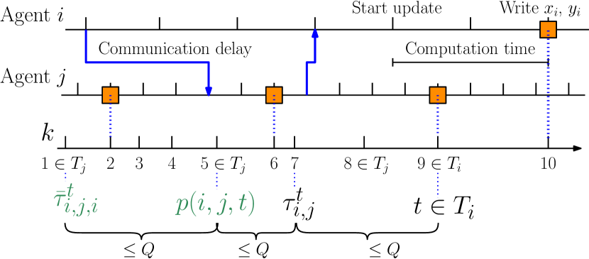
Figure 1: An example of asynchronous updates and communication. We consider a simple scenario, where each agent periodically broadcasts its variables and computes an update using the latest data received from its neighbors, according to its local clock. The communication is subject to bounded delays. The figure only considers two neighboring agents $i$ and $j$. The squares indicates the instants when the local variables change value; the arrows indicates data transmission. The global counter $k$ increases every time an agent in the network completes its update. Here, agent $i$ completes an update using the outdated information $x_{j}(7),y_{j}(7)$ and $k$ is increased to $10$: hence agent $i$ is viewed by an external observer as performing the update at $k=9$, and $\tau_{i,j}^{9}=7$. The quantities in green are defined in §IV.

We are ready to enunciate our main result.

Theorem 1

Let Assumptions 1-2 hold. For all ${i\in\mathcal{I}}$, let

$$\theta_{i} :=\sqrt{\textstyle\sum_{j\in\mathcal{N}_{i}}\theta_{j,i}^{2}}$$ (10)

$$\phi_{i} :=\textstyle\sum_{j\in\mathcal{N}_{i}}\frac{\theta_{j}^{2}}{\rho_{{\color[rgb]{0,0,0}i}}}$$ (11)

$$\ell_{i} :=\textstyle\sum_{j\in\mathcal{N}_{i}}\theta_{i,j}\frac{\theta_{j}}{\rho_{j}}$$ (12)

$$\xi_{i} :={\color[rgb]{0,0,0}\textstyle\sum_{j\in\mathcal{N}_{i}}\sum_{l\in\mathcal{N}_{j}}\theta_{l,j}{\textstyle\frac{\theta_{j}}{\rho_{j}}}}$$ (13)

with $\theta_{j,i}$ and $\rho_{j}$ as in Assumption 1, for all $i,j\in\mathcal{I}$. Assume that, for all ${i\in\mathcal{I}}$, the step size $\gamma_{i}>0$ is chosen such that

$$\textstyle\gamma_{i}^{-1}>\frac{1}{2}\phi_{i}+{\color[rgb]{0,0,0}\frac{3}{2}Q(\ell_{i}+\xi_{i})},$$ (14)

with $Q$ as in Assumption 2. Then, the sequence $(x(k))_{{k\in\mathbb{N}}}$ generated by Algorithm 1 converges to the solution $x^{\star}$ of the optimization problem in (1). $\square$

Remark 4

Each agent $i$ can locally compute the parameters $\phi_{i}$, $\ell_{i}$, $\xi_{i}$ in Theorem 1, only based on some information from its direct neighbors. Thus, the choice of the step sizes $\gamma_{i}$’s is decentralized, provided that the agents have access to (an upper bound for) the asynchronism bound $Q$ (otherwise, vanishing step sizes can be considered). $\square$

Remark 5

As usual for partially asynchronous optimization algorithms [13], [15], the upper bound in (14) decreases if $Q$ grows. This is a structural issue: we can construct a problem satisfying Assumption 1 (similarly to [13, §7.1, Ex.1.3]) such that, for any fixed positive $\gamma_{i}$’s, there is a large enough $Q$ and some sequences $\tau_{i,j}^{k}$’s , $T_{i}$’s satisfying Assumption 2, for which Algorithm 1 diverges. $\square$

IV Convergence analysis

In this section we prove Theorem 1. Our idea is to relate Algorithm 1 to a perturbed scaled block coordinate version of (5), and to show that, for small-enough steps sizes, the error caused by the outdated information is also small and does not compromise convergence. With respect to the asynchronous gradient method in [13], the main technical complication is that, for each update in (5), the agents communicate twice; in turn, the update of agent $i$ depends on the variables of its neighbors’ neighbors (or second order neighbors). In the following, we denote by $\stackon[.5pt]{y}{\scriptscriptstyle\sim}_{i}:=\mathrm{col}((y_{j})_{j\in\mathcal{N}_{i}})$ and $\stackon[-.5pt]{\stackon[.5pt]{y}{\scriptscriptstyle\sim}}{\scriptscriptstyle\sim}_{i}:=\mathrm{col}((\stackon[.5pt]{y}{\scriptscriptstyle\sim}_{j})_{j\in\mathcal{N}_{i}})$ the dual variables of the neighbors and second order neighbors of agent $i$, respectively.

To compare Algorithm 1 and (5), the first step is to get rid of the primal variables $x_{i}$’s in Algorithm 1. Importantly, we have to take into account that the $x_{j}$’s in (7b) are not only outdated, but also computed using outdated information. In fact, for any $i\in\mathcal{I}$, $k\in T_{i}$, the variable $x_{j}(\tau_{i,j}^{k})$ is computed by agent $j\in\mathcal{N}_{i}$, according to (7a), as

$$x_{j}(\tau_{i,j}^{k}) =\hphantom{:}\underset{x_{j}\in\mathbb{R}^{n_{j}}}{\mathop{\rm argmin}}\ f_{j}(x_{j})+\sum_{l\in\mathcal{N}_{j}}\langle g_{l,j}(x_{j}),y_{l}(\bar{\tau}^{k}_{i,j,l})\rangle$$ (15)

$$=:\mathbbm{x}^{\star}_{j}(\stackon[.5pt]{y}{\scriptscriptstyle\sim}_{j}(\bar{\tau}^{k}_{i,j})),$$ (16)

where, for all $l\in\mathcal{N}_{j}$, $\bar{\tau}^{k}_{i,j,l}:={\tau}^{p}_{j,l}$, and $p$ is the last time agent $j$ performed an update prior to $\tau_{i,j}^{k}$ (see Figure 1), i.e.,

$$p=p(i,j,k):=\max(\{0\}\cup\{t\in T_{j}\mid t\leq\tau_{i,j}^{k}-1\}),$$ (17)

(and (15) also holds if $p(i,j,k)=0$ because of the initial conditions in Algorithm 1). For brevity of notation, in (16), we define $\bar{\tau}^{k}_{i,j}:=\mathrm{col}((\bar{\tau}^{k}_{i,j,l})_{l\in\mathcal{N}_{j}})$ and $\stackon[.5pt]{y}{\scriptscriptstyle\sim}_{j}(\bar{\tau}^{k}_{i,j}):=\mathrm{col}((y_{l}(\bar{\tau}^{k}_{i,j,l})_{l\in\mathcal{N}_{j}})$. By replacing (16) in (7a), we obtain that, for all ${i\in\mathcal{I}}$, $k\in T_{i}$

$$y_{i}(k+1) =\hphantom{:}{\mathrm{proj}}_{\Omega_{i}}\Biggl{(}\ y_{i}(k)+\gamma_{i}\sum_{j\in\mathcal{N}_{i}}g_{i,j}(\mathbbm{x}^{\star}_{j}(\stackon[.5pt]{y}{\scriptscriptstyle\sim}_{j}(\bar{\tau}^{k}_{i,j})))\Biggr{)}$$

$$=:{\mathrm{proj}}_{\Omega_{i}}\left(\ y_{i}(k)+\gamma_{i}\boldsymbol{F}_{i}(\stackon[-.5pt]{\stackon[.5pt]{y}{\scriptscriptstyle\sim}}{\scriptscriptstyle\sim}_{i}(\bar{\tau}^{k}_{i}))\right),$$ (18)

where $\bar{\tau}_{i}^{k}:=\mathrm{col}((\bar{\tau}^{k}_{i,j})_{j\in\mathcal{N}_{i}})$, $\stackon[-.5pt]{\stackon[.5pt]{y}{\scriptscriptstyle\sim}}{\scriptscriptstyle\sim}_{i}(\bar{\tau}_{i}^{k}):=\mathrm{col}((\stackon[.5pt]{y}{\scriptscriptstyle\sim}_{j}(\bar{\tau}^{k}_{i,j}))_{j\in\mathcal{N}_{i}})$. Hence, (18) expresses the update in (7b) as a function of the outdated dual variables of the second order neighbors of agent $i$. Since (18) makes use of second order information, the maximum delay (in this notation) is not bounded by $Q$ anymore: instead, by (17) and Assumption 2, it holds that $p(i,j,k)-Q\leq\tau_{j,l}^{p(i,j,k)}=\bar{\tau}_{i,j,l}^{k}\leq p(i,j,k)$, $\tau^{k}_{i,j}-Q\leq p(i,j,k)\leq\max(0,\tau^{k}_{i,j}-1)$, $k-Q\leq\tau^{k}_{i,j}\leq k$; thus,

$$k-3Q\leq\bar{\tau}^{k}_{i,j,l}\leq k-1,$$ (19)

for all $k\geq 1$, and $\bar{\tau}^{0}_{i,j,l}=0$. Figure 1 illustrates how the lower bound is obtained, with $l=i$.

We emphasize that the mapping $\boldsymbol{F}_{i}$ is not a partial gradient of the dual function (differently from the asynchronous gradient method in [13]) – e.g., its argument lies in a different space. In particular, we note that $\stackon[-.5pt]{\stackon[.5pt]{y}{\scriptscriptstyle\sim}}{\scriptscriptstyle\sim}_{i}(\bar{\tau}^{k}_{i})$ can contain multiple instances of $y_{l}$, for some $l\in\mathcal{I}$ (including $y_{i}$), with different delays. Nonetheless, by the definition in (18), for any $y(k)\in\mathbb{R}^{m}$, we have

$$\boldsymbol{F}_{i}(\stackon[-.5pt]{\stackon[.5pt]{y}{\scriptscriptstyle\sim}}{\scriptscriptstyle\sim}_{i}(k))=\nabla_{y_{i}}q(y(k)).$$ (20)

In one word, if there is no delay, (18) corresponds to the $y_{i}$-update of the synchronous dual ascent (5) (however, there is always delay in Algorithm 1, see (19) and Remark 2).

Finally, we can also rewrite Algorithm 1 as

$$(\forall{k\in\mathbb{N}})(\forall{i\in\mathcal{I}})\quad y_{i}(k+1)=y_{i}(k)+\gamma_{i}s_{i}(k),$$ (21)

where

$$s_{i}(k):=\frac{1}{\gamma_{i}}({\mathrm{proj}}_{\Omega_{i}}(\ y_{i}(k)+\gamma_{i}\boldsymbol{F}_{i}(\stackon[-.5pt]{\stackon[.5pt]{y}{\scriptscriptstyle\sim}}{\scriptscriptstyle\sim}_{i}(\bar{\tau}^{k}_{i})))-y_{i}(k)),$$ (22)

if $k\in T_{i}$, $s_{i}(k)=\boldsymbol{0}_{m_{i}}$ otherwise.

Before proceeding with the analysis of Theorem 1, we recall the following results. The proof of Lemma 1 is standard and omitted here (see, e.g., [9, Lem. 1]).

Lemma 1

For all $j\in\mathcal{I}$, the mapping $\mathbbm{x}^{\star}_{j}$ in (16) is $\frac{\theta_{j}}{\rho_{j}}$-Lipschitz continuous, with $\theta_{j}$ as in (10). $\square$

Lemma 2 (Weighted descent lemma, [6, Lem. 2.2])

Let $\Phi=\mathop{\hbox{\rm diag}}((\phi_{i}\otimes I_{m_{i}})_{i\in\mathcal{I}})$, $\phi_{i}$ as in (11), for all ${i\in\mathcal{I}}$. Let $q$ be the dual function in (4). For any $y,z\in\mathbb{R}^{m}$, it holds that

$$q(y)\geq q(z)+\langle y-z,\nabla q(z)\rangle-\textstyle\frac{1}{2}\|y-z\|^{2}_{\Phi}.$$

Lemma 3 ([13, Lemma 5.1])

Let $s_{i}(k)$ be as in (22), for all ${i\in\mathcal{I}}$. Then, for all ${i\in\mathcal{I}}$, ${k\in\mathbb{N}}$, it holds that

$$\langle s_{i}(k),\boldsymbol{F}_{i}(\stackon[-.5pt]{\stackon[.5pt]{y}{\scriptscriptstyle\sim}}{\scriptscriptstyle\sim}_{i}(\bar{\tau}^{k}_{i}))\rangle\geq\|s_{i}(k)\|^{2}.$$

IV-A Proof of Theorem 1

Let $\Gamma:=\mathop{\hbox{\rm diag}}((\gamma_{i}\otimes I_{m_{i}})_{{i\in\mathcal{I}}})$, $s(k)=\mathrm{col}((s_{i}(k))_{k\in\mathbb{N}})$, $\boldsymbol{F}(\stackon[-.5pt]{\stackon[.5pt]{y}{\scriptscriptstyle\sim}}{\scriptscriptstyle\sim}(\bar{\tau}^{k})):=\mathrm{col}((\boldsymbol{F}_{i}(\stackon[-.5pt]{\stackon[.5pt]{y}{\scriptscriptstyle\sim}}{\scriptscriptstyle\sim}_{i}(\bar{\tau}^{k}_{i})))_{{i\in\mathcal{I}}})$. By Lemma 2, we have

$$q(y(k+1)) =q(y(k)+\Gamma s(k))$$

$$\geq q(y(k))-\textstyle\frac{1}{2}\|\Gamma s(k)\|^{2}_{\Phi}+\langle\Gamma s(k),\nabla q(y(k))\rangle$$

$$=q(y(k))-\textstyle\frac{1}{2}\|\Gamma s(k)\|^{2}_{\Phi}+\langle\Gamma s(k),\boldsymbol{F}(\stackon[-.5pt]{\stackon[.5pt]{y}{\scriptscriptstyle\sim}}{\scriptscriptstyle\sim}(\bar{\tau}^{k}))\rangle$$

$$\qquad+\langle\Gamma s(k),\nabla q(y(k))-\boldsymbol{F}(\stackon[-.5pt]{\stackon[.5pt]{y}{\scriptscriptstyle\sim}}{\scriptscriptstyle\sim}(\bar{\tau}^{k}))\rangle$$

$$=q(y(k))-\textstyle\frac{1}{2}\|\Gamma s(k)\|^{2}_{\Phi}+\langle\Gamma s(k),\boldsymbol{F}(\stackon[-.5pt]{\stackon[.5pt]{y}{\scriptscriptstyle\sim}}{\scriptscriptstyle\sim}(\bar{\tau}^{k}))\rangle$$

$$\qquad+\langle\Gamma s(k),\boldsymbol{F}(\stackon[-.5pt]{\stackon[.5pt]{y}{\scriptscriptstyle\sim}}{\scriptscriptstyle\sim}(k))-\boldsymbol{F}(\stackon[-.5pt]{\stackon[.5pt]{y}{\scriptscriptstyle\sim}}{\scriptscriptstyle\sim}(\bar{\tau}^{k}))\rangle$$

$$\geq q(y(k))-\textstyle\frac{1}{2}\|s(k)\|^{2}_{\Phi\Gamma^{2}}+\|s(k)\|_{\Gamma}^{2}$$

$$\qquad+\langle\Gamma s(k),\boldsymbol{F}(\stackon[-.5pt]{\stackon[.5pt]{y}{\scriptscriptstyle\sim}}{\scriptscriptstyle\sim}(k))-\boldsymbol{F}(\stackon[-.5pt]{\stackon[.5pt]{y}{\scriptscriptstyle\sim}}{\scriptscriptstyle\sim}(\bar{\tau}^{k}))\rangle,$$ (23)

where in the last equality we used (20) and the last inequality follows by Lemma 3 (we recall that $\Phi,\Gamma$ are diagonal matrices). We next bound the last addend in (23). By definition of $\boldsymbol{F}_{i}$ in (18) and the Cauchy–Schwartz inequality, we have

$$\langle\Gamma s(k),\boldsymbol{F}(\stackon[-.5pt]{\stackon[.5pt]{y}{\scriptscriptstyle\sim}}{\scriptscriptstyle\sim}(k))-\boldsymbol{F}(\stackon[-.5pt]{\stackon[.5pt]{y}{\scriptscriptstyle\sim}}{\scriptscriptstyle\sim}(\bar{\tau}^{k}))\rangle$$

$$\geq-\sum_{{i\in\mathcal{I}}}\|\gamma_{i}s_{i}(k)\|\|\boldsymbol{F}_{i}(\stackon[-.5pt]{\stackon[.5pt]{y}{\scriptscriptstyle\sim}}{\scriptscriptstyle\sim}_{i}(k))-\boldsymbol{F}_{i}(\stackon[-.5pt]{\stackon[.5pt]{y}{\scriptscriptstyle\sim}}{\scriptscriptstyle\sim}_{i}(\bar{\tau}^{k}_{i}))\|$$

$$\geq-\sum_{{i\in\mathcal{I}}}\|\gamma_{i}s_{i}(k)\|\!\sum_{j\in\mathcal{N}_{i}}\!\!\|g_{i,j}(\mathbbm{x}^{\star}_{j}(\stackon[.5pt]{y}{\scriptscriptstyle\sim}_{j}(k)))\!-\!g_{i,j}(\mathbbm{x}^{\star}_{j}(\stackon[.5pt]{y}{\scriptscriptstyle\sim}_{j}(\bar{\tau}^{k}_{i,j})))\|$$

$$\geq-\sum_{{i\in\mathcal{I}}}\|\gamma_{i}s_{i}(k)\|\sum_{j\in\mathcal{N}_{i}}\theta_{i,j}{\textstyle\frac{\theta_{j}}{\rho_{j}}}\ \|\stackon[.5pt]{y}{\scriptscriptstyle\sim}_{j}(k)-\stackon[.5pt]{y}{\scriptscriptstyle\sim}_{j}(\bar{\tau}^{k}_{i,j})\|$$

$$\geq-\sum_{{i\in\mathcal{I}}}\|\gamma_{i}s_{i}(k)\|\sum_{j\in\mathcal{N}_{i}}\theta_{i,j}{\textstyle\frac{\theta_{j}}{\rho_{j}}}\sum_{\tau=k-3Q}^{k-1}\!\!\|\mathrm{col}((\gamma_{l}s_{l}(\tau))_{l\in\mathcal{N}_{j}})\|,$$

where in the third inequality we used Lemma 1 and Assumption 1(ii), and the last follows by (21) and (19) (without loss of generality, we let $s(k):=\boldsymbol{0}_{m}$, for all $k<0$). Therefore, by the elementary relation $2|a||b|\leq a^{2}+b^{2}$, we obtain

$$\langle\Gamma s(k),\boldsymbol{F}(\stackon[-.5pt]{\stackon[.5pt]{y}{\scriptscriptstyle\sim}}{\scriptscriptstyle\sim}(k))-\boldsymbol{F}(\stackon[-.5pt]{\stackon[.5pt]{y}{\scriptscriptstyle\sim}}{\scriptscriptstyle\sim}(\bar{\tau}^{k}))\rangle$$

$$\quad\geq-\sum_{\tau=k-3Q}^{k-1}\sum_{{i\in\mathcal{I}}}\sum_{j\in\mathcal{N}_{i}}\theta_{i,j}{\textstyle\frac{\theta_{j}}{\rho_{j}}}\ {\textstyle\frac{1}{2}}\|\gamma_{i}s_{i}(k)\|^{2}$$

$$\hphantom{{}\leq{}}\quad-\sum_{\tau=k-3Q}^{k-1}\sum_{{i\in\mathcal{I}}}\sum_{j\in\mathcal{N}_{i}}\theta_{i,j}{\textstyle\frac{\theta_{j}}{\rho_{j}}}\sum_{l\in\mathcal{N}_{j}}{\textstyle\frac{1}{2}}\|\gamma_{l}s_{l}(\tau)\|^{2}.$$ (24)

The first term on the right-hand side of (24) equals $-\|s(k)\|^{2}_{\frac{3}{2}Q\Gamma^{2}L}$, with $L:=\mathop{\hbox{\rm diag}}((\ell_{i}\otimes I_{m_{i}})_{i\in\mathcal{I}})$ and $\ell_{i}$ as in (12). For the second term, since $\mathcal{G}$ is undirected, we reorder the addends as

$$\sum_{\tau=k-3Q}^{k-1}\sum_{{i\in\mathcal{I}}}\sum_{j\in\mathcal{N}_{i}}\theta_{i,j}{\textstyle\frac{\theta_{j}}{\rho_{j}}}\sum_{l\in\mathcal{N}_{j}}{\textstyle\frac{1}{2}}\|\gamma_{l}s_{l}(\tau)\|^{2}$$

$$\quad=\sum_{\tau=k-3Q}^{k-1}\sum_{{i\in\mathcal{I}}}{\textstyle\frac{1}{2}}\|\gamma_{i}s_{i}(\tau)\|^{2}\left(\sum_{j\in\mathcal{N}_{i}}\sum_{l\in\mathcal{N}_{j}}\theta_{l,j}{\textstyle\frac{\theta_{j}}{\rho_{j}}}\right)$$

$$\quad=\sum_{\tau=k-3Q}^{k-1}\|s(\tau)\|^{2}_{{\frac{1}{2}}\Gamma^{2}\Xi},$$

where $\Xi=:\mathop{\hbox{\rm diag}}((\xi_{i}\otimes I_{m_{i}})_{i\in\mathcal{I}})$ and $\xi_{i}$ as in (13). Then, by substituting in (23), we obtain

$$q(y(k+1)) \geq q(y(k))+\|s(k)\|^{2}_{\Gamma(I-\frac{1}{2}\Phi\Gamma-\frac{3}{2}QL\Gamma)}$$

$$\qquad-\sum_{\tau=k-3Q}^{k-1}\|s(\tau)\|^{2}_{{\textstyle\frac{1}{2}}\Xi\Gamma^{2}},$$ (25)

with $I-\frac{1}{2}\Phi\Gamma-\frac{3}{2}QL\Gamma\succ 0$ by the assumption on $\Gamma$ in (14). Since (25) holds for any $k$, summing over $k$ finally yields

$$q(y(k+1))-q(y(0))$$

$$\qquad\geq\sum_{\tau=0}^{k}\|s(\tau)\|^{2}_{\Gamma(I-\frac{1}{2}\Phi\Gamma-\frac{3}{2}QL\Gamma)}-3Q\sum_{\tau=0}^{k}\|s(\tau)\|^{2}_{\frac{1}{2}\Xi\Gamma^{2}}$$

$$\qquad=\sum_{\tau=0}^{k}\|s(\tau)\|^{2}_{\Gamma(I-\frac{1}{2}\Phi\Gamma-\frac{3}{2}Q(\Xi+L)\Gamma)},$$ (26)

and $I-\frac{1}{2}\Phi\Gamma-\frac{3}{2}Q(\Xi+L)\Gamma\succ 0$ by assumption (14).

We know that $q$ is bounded above on $\Omega$ by (3), and $y(k)\in\Omega\$ for all ${k\in\mathbb{N}}$; then, by taking the limit in (26), we have

$$\lim_{k\to\infty}s(k)=\boldsymbol{0}_{m}.$$ (27)

Hence, by the updates in (21) and by (27), we also have

$$\lim_{k\to\infty}\|y(k+1)-y(k)\|=0.$$ (28)

Similarly, since, by Assumption 2(ii) and (21), $\|y_{j}(k)-y_{j}(\tau^{k}_{i,j})\|\leq\sum_{\tau=k-Q}^{k-1}\gamma_{j}\|s_{j}(\tau)\|$, it also follows that

$$\lim_{k\to\infty}\|y_{j}(k)-y_{j}(\tau^{k}_{i,j})\|=0,\ \forall{i\in\mathcal{I}},j\in\mathcal{N}_{i}.$$ (29)

For any ${i\in\mathcal{I}}$, consider the subsequence $(s_{i}(k))_{k\in T_{i}}$, which converges to $\boldsymbol{0}$ by (27). In view of (22), $({\mathrm{proj}}_{\Omega_{i}}(\ y_{i}(k)+\gamma_{i}\boldsymbol{F}_{i}(\stackon[-.5pt]{\stackon[.5pt]{y}{\scriptscriptstyle\sim}}{\scriptscriptstyle\sim}_{i}(\bar{\tau}^{k}_{i})))-y_{i}(k))_{k\in T_{i}}\rightarrow\boldsymbol{0}$. Therefore, by leveraging the continuity of $\boldsymbol{F}_{i}$ (which directly follows by the definition in (18) and Lemma 1) and of the projection [13, §3.3, Prop. 3.2], (29) and (20) yield $({\mathrm{proj}}_{\Omega_{i}}(\ y_{i}(k)+\gamma_{i}\nabla_{y_{i}}q(y(k))-y_{i}(k)))_{k\in T_{i}}\rightarrow\boldsymbol{0}$. However, again by continuity, (28) and Assumption 2(i), we can also infer convergence of the whole sequence, $\lim_{k\to\infty}\ {\mathrm{proj}}_{\Omega_{i}}(\ y_{i}(k)+\gamma_{i}\nabla_{y_{i}}q(y(k))-y_{i}(k)=\boldsymbol{0}_{m_{i}}$, or

$$\lim_{k\to\infty}\ \left({\mathrm{proj}}_{\Omega_{i}}(\ y(k)+\Gamma\nabla q(y(k))-y(k)\right)=\boldsymbol{0}_{m}.$$ (30)

We note that $q(y(k))\geq q(y(0))$ for all ${k\in\mathbb{N}}$, by (26); moreover, $-q$ is coercive on $\Omega$ by Assumption 1(iii) and 1(iv). We conclude that the sequence $(y(k))_{k\in\mathbb{N}}$ is bounded; in turn, (30) implies that $(y(k))_{k\in\mathbb{N}}$ converges to the set of dual solutions $\mathcal{Y}^{\star}$.

We can finally turn our attention to the primal problem (1). By (7a), for any ${i\in\mathcal{I}}$, $k\in T_{i}$, we have $x_{i}(k+1)=\mathbbm{x}^{\star}_{i}(\stackon[.5pt]{y}{\scriptscriptstyle\sim}_{i}(\tau_{i}^{k}))$, where $\mathbbm{x}^{\star}_{i}$ is defined in (16) and $\tau_{i}^{k}:=\mathrm{col}((\tau_{i,j}^{k})_{j\in\mathcal{N}_{i}})$. Moreover, by strong duality, for any $y^{\star}=\mathrm{col}((y_{i}^{\star})_{i\in\mathcal{I}})\in\mathcal{Y^{\star}}$, it holds that $\mathbbm{x}^{\star}_{i}(\stackon[.5pt]{y}{\scriptscriptstyle\sim}_{i}^{\star})=x_{i}^{\star}$, with $\stackon[.5pt]{y}{\scriptscriptstyle\sim}_{i}^{\star}:=\mathrm{col}((y_{j}^{\star})_{j\in\mathcal{N}_{i}})$ and $\mathrm{col}((x_{i}^{\star})_{i\in\mathcal{I}})=x^{\star}$. Therefore we can exploit (29), the fact that $(y(k))_{k}$ is converging to $\mathcal{Y}^{\star}$, and Lipschitz continuity of $\mathbbm{x}^{\star}_{i}$ in Lemma 1, to conclude that $(x_{i}(k+1))_{k\in T_{i}}\rightarrow x_{i}^{\star}$. The conclusion follows because the convergence also holds for the whole sequence, i.e., $(x_{i}(k))_{{k\in\mathbb{N}}}\rightarrow x_{i}^{\star}$, by (8a). $\blacksquare$

V Numerical simulation

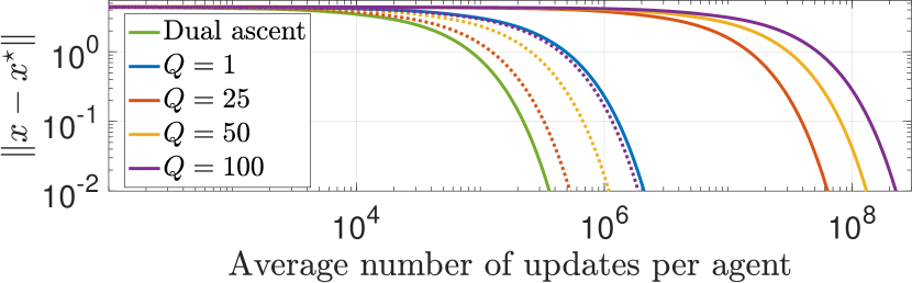
Figure 2: Distance from the optimum, with step sizes chosen to satisfy their theoretical upper bounds (solid lines) and $100$ times larger (dotted lines).

We consider an OPF problem on the IEEE 14-bus network [9, Fig. 2]. Each bus $i\in\mathcal{I}=\{1,\dots,14\}$ has a decision variable $x_{i}=\mathrm{col}(P_{i},\psi_{i})\in\mathbb{R}^{2}$, where $P_{i}\geq 0$ is the power generated, bounded by generation capacities, and $\psi_{i}$ is the voltage phase of bus $i$. The goal is to minimize the sum of strongly convex quadratic local costs, subject to the coupling flow constraints $\{P_{i}-P_{i}^{\text{d}}=\textstyle\sum_{j\in\mathcal{N}_{i}}B_{i,j}(\psi_{i}-\psi_{j}),\forall{i\in\mathcal{I}}\}$, where $P_{i}^{\text{d}}\geq 0$ is the power demand at bus $i$ and $B_{i,j}$ is the susceptance of line $(i,j)$, which represent the direct current approximation of the power flow equations. We simulate Algorithm 1 for the setup in Figure 1, with randomly chosen delays and local clock frequencies. We compare four scenarios, resulting in different values for $Q$, with the synchronous dual ascent (6), in Figure 2. The case $Q=1$ corresponds to a synchronous algorithm, where all the agents update their variables at every iteration. For $Q>1$, the agents perform updates asynchronously, according to their own clocks. To compare synchronous and asynchronous implementation, we take into account the overall computation burden, i.e., the average number of updates performed per agent. For large values of $Q$, the upper bounds on the step sizes $\gamma_{i}$’s in (14) decrease, resulting in slower convergence. However, the bounds can be conservative. In fact, Algorithm 1 still converges with step sizes set $100$ times larger than their theoretical upper bounds for $Q=25,50,100$ (but not for $Q=1$).

VI Conclusion

The distributed dual ascent retains its convergence properties even if the updates are carried out completely asynchronously and using delayed information, provided that small enough uncoordinated step sizes are chosen. Convergence rates for primal-dual methods in this general asynchronous scenario are currently unknown.

References

- [1] D. K. Molzahn, F. Dörfler, H. Sandberg, S. H. Low, S. Chakrabarti, R. Baldick, and J. Lavaei, “A survey of distributed optimization and control algorithms for electric power systems,” IEEE Transactions on Smart Grid, vol. 8, no. 6, pp. 2941–2962, 2017.
- [2] Li Xiao, M. Johansson, and S. P. Boyd, “Simultaneous routing and resource allocation via dual decomposition,” IEEE Transactions on Communications, vol. 52, no. 7, pp. 1136–1144, 2004.
- [3] S. Boyd, N. Parikh, E. Chu, B. Peleato, and J. Eckstein, “Distributed optimization and statistical learning via the alternating direction method of multipliers,” Foundations and Trends in Machine Learning, vol. 3, no. 1, p. 1–122, 2010.
- [4] M. G. Rabbat and R. D. Nowak, “Decentralized source localization and tracking [wireless sensor networks],” in IEEE International Conference on Acoustics, Speech, and Signal Processing, vol. 3, 2004, pp. 921–924.
- [5] H. Everett, “Generalized Lagrange multiplier method for solving problems of optimum allocation of resources,” Operations Research, vol. 11, no. 3, pp. 399–417, 1963.
- [6] I. Necoara and V. Nedelcu, “On linear convergence of a distributed dual gradient algorithm for linearly constrained separable convex problems,” Automatica, vol. 55, pp. 209–216, 2015.
- [7] A. Beck, A. Nedić, A. Ozdaglar, and M. Teboulle, “An gradient method for network resource allocation problems,” IEEE Transactions on Control of Network Systems, vol. 1, no. 1, pp. 64–73, 2014.
- [8] A. Nedić and A. Ozdaglar, “Approximate primal solutions and rate analysis for dual subgradient methods,” SIAM Journal on Optimization, vol. 19, no. 4, p. 1757–1780, 2009.
- [9] W. Ananduta, C. Ocampo-Martinez, and A. Nedić, “Accelerated multi-agent optimization method over stochastic networks,” in 59th IEEE Conference on Decision and Control (CDC), 2020, pp. 2961–2966.
- [10] A. Camisa, F. Farina, I. Notarnicola, and G. Notarstefano, “Distributed constraint-coupled optimization over random time-varying graphs via primal decomposition and block subgradient approaches,” in 58th IEEE Conference on Decision and Control, 2019, pp. 6374–6379.
- [11] A. Falsone and M. Prandini, “A distributed dual proximal minimization algorithm for constraint-coupled optimization problems,” IEEE Control Systems Letters, vol. 5, no. 1, pp. 259–264, 2021.
- [12] X. Li, G. Feng, and L. Xie, “Distributed proximal algorithms for multiagent optimization with coupled inequality constraints,” IEEE Transactions on Automatic Control, vol. 66, no. 3, pp. 1223–1230, 2021.
- [13] D. P. Bertsekas and J. N. Tsitsiklis, Parallel and distributed computation: numerical methods. Prentice hall, 1989, vol. 23.
- [14] K. Srivastava and A. Nedić, “Distributed asynchronous constrained stochastic optimization,” IEEE Journal of Selected Topics in Signal Processing, vol. 5, no. 4, pp. 772–790, 2011.
- [15] Y. Tian, Y. Sun, and G. Scutari, “Achieving linear convergence in distributed asynchronous multiagent optimization,” IEEE Transactions on Automatic Control, vol. 65, no. 12, pp. 5264–5279, 2020.
- [16] I. Notarnicola, R. Carli, and G. Notarstefano, “Distributed partitioned big-data optimization via asynchronous dual decomposition,” IEEE Transactions on Control of Network Systems, vol. 5, no. 4, pp. 1910–1919, 2018.
- [17] N. Bastianello, R. Carli, L. Schenato, and M. Todescato, “Asynchronous distributed optimization over lossy networks via relaxed ADMM: Stability and linear convergence,” IEEE Transactions on Automatic Control, 2020, doi: 10.1109/TAC.2020.3011358.
- [18] Y. Lin, I. Shames, and D. Nešić, “Asynchronous distributed optimization via dual decomposition and block coordinate ascent,” in 58th IEEE Conference on Decision and Control (CDC), 2019, pp. 6380–6385.
- [19] F. Farina, A. Garulli, A. Giannitrapani, and G. Notarstefano, “A distributed asynchronous method of multipliers for constrained nonconvex optimization,” Automatica, vol. 103, pp. 243–253, 2019.
- [20] T. Wu, K. Yuan, Q. Ling, W. Yin, and A. H. Sayed, “Decentralized consensus optimization with asynchrony and delays,” IEEE Transactions on Signal and Information Processing over Networks, vol. 4, no. 2, pp. 293–307, 2018.
- [21] T. Chang, M. Hong, W. Liao, and X. Wang, “Asynchronous distributed ADMM for large-scale optimization—Part I: Algorithm and convergence analysis,” IEEE Transactions on Signal Processing, vol. 64, no. 12, pp. 3118–3130, 2016.
- [22] Z. Peng, Y. Xu, M. Yan, and W. Yin, “ARock: An algorithmic framework for asynchronous parallel coordinate updates,” SIAM Journal on Scientific Computing, vol. 38, no. 5, pp. A2851–A2879, 2016.
- [23] S. H. Low and D. E. Lapsley, “Optimization flow control. I. Basic algorithm and convergence,” IEEE/ACM Transactions on Networking, vol. 7, no. 6, pp. 861–874, 1999.
- [24] R. Hannah and W. Yin, “On unbounded delays in asynchronous parallel fixed-point algorithms,” Journal of Scientific Computing volume, vol. 76, p. 299–326, 2018.
- [25] R. T. Rockafellar, Network Flows and Monotropic Optimization. Athena Scientific, 1998.
- [26] ——, Convex Analysis. Princeton University Press, 1970.
- [27] J. Hiriart-Urruty and C. Lemaréchal, Fundamentals of convex analysis. Springer Science & Business Media, 2012.