Linear response theory and damped modes of stellar clusters

Abstract

Because all stars contribute to its gravitational potential, stellar clusters amplify perturbations collectively. In the limit of small fluctuations, this is described through linear response theory, via the so-called response matrix. While the evaluation of this matrix is somewhat straightforward for unstable modes (i.e. with a positive growth rate), it requires a careful analytic continuation for damped modes (i.e. with a negative growth rate). We present a generic method to perform such a calculation in spherically symmetric stellar clusters. When applied to an isotropic isochrone cluster, we recover the presence of a low-frequency weakly damped ${\ell\!=\!1}$ mode. We finally use a set of direct $N$-body simulations to test explicitly this prediction through the statistics of the correlated random walk undergone by a cluster’s density centre.

1 Introduction

All the stars in a stellar cluster contribute collectively to the system’s potential. This self-consistency naturally allows the cluster to respond and amplify disturbances. In the limit of small perturbations, this is described by linear response theory (see, e.g., Binney & Tremaine, 2008). Such a generic machinery is paramount to characterise a cluster’s possible unstable modes, i.e. with an amplitude growing exponentially in time, for example via the radial-orbit instability in radially anisotropic stellar clusters (see, e.g., Merritt, 1999; Maréchal & Perez, 2011, for reviews).

Yet, even if a cluster is dynamically stable, i.e. there are no unstable modes, it does not imply that it is dynamically static. Indeed, the cluster can still sustain damped modes, i.e. with an amplitude decaying exponentially in time. These are commonly called Landau damped modes, and require a careful analytic continuation of the response matrix following Landau’s prescription. While these modes naturally damp when in isolation, they can also be excited by external perturbations, e.g., fly-bys (Weinberg, 1989) or continuously seeded by the cluster’s intrinsic thermal Poisson shot noise (Weinberg, 1998).

The importance of these damped modes in globular clusters is the clearest through its ${\ell\!=\!1}$ ‘sloshing’ mode that induces slow long-lasting oscillations of a cluster’s centre (see, e.g., Heggie et al., 2020, and references therein), and is also imprinted through the strong amplification of large-scale dipole fluctuations (Weinberg, 1998; Hamilton et al., 2018; Lau & Binney, 2019). In a seminal work, Weinberg (1994) developed an elegant numerical procedure to systematically evaluate a cluster’s response matrix for such damped frequencies. This is the problem that we revisit here putting forward a different approach to perform efficiently and explicitly this analytic continuation.

The present paper is organised as follows. In §2, we briefly review the linear response theory of stellar systems. In §3, we rewrite the cluster’s response matrix to perform its analytic continuation necessary to capture the damped part of the modes’ spectrum. We apply this method in §4 to the isotropic isochrone cluster and recover the presence of a weakly damped ${\ell\!=\!1}$ mode therein, which is subsequently compared with direct $N$-body simulations. Finally, we conclude in §5. In all these sections, technical details are either deferred to Appendices or to appropriate references.

2 Linear response theory

The linear response theory of an integrable long-range interacting system of dimension $d$ is generically characterised by its response matrix, ${\mathbf{M}(\omega)}$ (see §5.3 in Binney & Tremaine, 2008), reading

$$M_{\alpha\beta}(\omega)=-(2\pi)^{d}\sum_{\mathbf{n}\in\mathbb{Z}^{d}}\int_{\begin{subarray}{c}\\[2.50153pt] \hphantom{-1}\\ \mathcal{L}\end{subarray}}^{\hphantom{1}}\!\!\!\!\mathrm{d}\mathbf{J}\,\frac{\mathbf{n}\!\cdot\!\partial F_{\mathrm{tot}}/\partial\mathbf{J}}{\mathbf{n}\!\cdot\!\mathbf{\Omega}(\mathbf{J})-\omega}\,\psi^{(\alpha)*}_{\mathbf{n}}(\mathbf{J})\,\psi^{(\beta)}_{\mathbf{n}}(\mathbf{J}).$$ (1)

In that expression, we introduced angle-action coordinates (of dimension $d$) as ${(\bm{\theta},\mathbf{J})}$, and the system’s quasi-stationary distribution function (DF), ${F_{\mathrm{tot}}(\mathbf{J})}$, normalised so that ${\!\int\!\mathrm{d}\bm{\theta}\mathrm{d}\mathbf{J}F_{\mathrm{tot}}\!=\!M}$, with $M$ the system’s total active mass. Equation (1) contains the orbital frequencies, ${\mathbf{\Omega}(\mathbf{J})}$, as well as the Fourier resonance numbers ${\mathbf{n}\!\in\!\mathbb{Z}^{d}}$. Finally, following the basis method (see §A), Eq. (1) also involves a set of biorthogonal potential basis elements, ${\psi^{(\alpha)}}$.

A system sustains a mode at the (complex) frequency $\omega$, if one has ${\det[\mathbf{I}\!-\!\mathbf{M}(\omega)]\!=\!0}$, with $\mathbf{I}$ the identity matrix. Here, the sign of ${\mathrm{Im}[\omega]}$ controls the nature of the mode, as ${\mathrm{Im}[\omega]\!>\!0}$ corresponds to unstable modes, ${\mathrm{Im}[\omega]\!=\!0}$ to neutral modes, and ${\mathrm{Im}[\omega]\!<\!0}$ to (Landau) damped ones. We refer to Case (1959); Lee (2018); Polyachenko et al. (2021); Lau & Binney (2021) and references therein for detailed discussions on the subtle distinction between genuine (van Kampen) modes and the present Landau damped modes.

Importantly, for ${\mathrm{Im}[\omega]\!<\!0}$ the action integral from Eq. (1) must be computed using Landau’s prescription (see, e.g., §5.2.4 in Binney & Tremaine, 2008), hence the notation ${\!\int_{\mathcal{L}}\mathrm{d}\mathbf{J}}$. In the case of ${1D}$ homogeneous system, this prescription takes the simple form

$$\int_{\begin{subarray}{c}\\[2.50153pt] -\infty\\ \mathcal{L}\end{subarray}}^{+\infty}\!\!\!\!\!\!\!\!\mathrm{d}u\,\frac{G(u)}{u\!-\!\omega}=\begin{cases}\displaystyle\!\!\int_{-\infty}^{+\infty}\!\!\!\!\!\!\!\!\mathrm{d}u\,\frac{G(u)}{u\!-\!\omega}&\!\!\!\text{if}\;\;\mathrm{Im}[\omega]>0,\\[8.61108pt] \displaystyle\mathcal{P}\!\!\int_{-\infty}^{+\infty}\!\!\!\!\!\!\!\!\mathrm{d}u\,\frac{G(u)}{u\!-\!\omega}+\mathrm{i}\pi\,G(\omega)&\!\!\!\text{if}\;\;\mathrm{Im}[\omega]=0,\\[8.61108pt] \displaystyle\!\!\int_{-\infty}^{+\infty}\!\!\!\!\!\!\!\!\mathrm{d}u\,\frac{G(u)}{u-\omega}+2\mathrm{i}\pi\,G(\omega)&\!\!\!\text{if}\;\;\mathrm{Im}[\omega]<0\end{cases}$$ (2)

where the function ${u\!\mapsto\!G(u)}$ is assumed to be analytic, e.g., ${G(u)\!\propto\!u\,\mathrm{e}^{-u^{2}}}$ in the case of a Maxwellian distribution. In Eq. (2), we also introduced $\mathcal{P}$ as Cauchy’s principal value. Our goal is to illustrate how one may adapt Landau’s prescription to the case of self-gravitating systems.

We now focus our interest on spherically symmetric stellar systems. In that case, as detailed in §4 of Hamilton et al. (2018), the response matrix from Eq. (1) decouples the various spherical harmonics ${\ell\!\geq\!0}$ from one another. The response matrix is then limited to a ${2D}$ action integral. For a given harmonic $\ell$, Eq. (1) generically takes the form

$$M^{\ell}_{pq}(\omega)=\sum_{\mathbf{n}\in\mathbb{Z}^{2}}\int_{\begin{subarray}{c}\\[2.50153pt] \hphantom{-1}\\ \mathcal{L}\end{subarray}}^{\hphantom{1}}\!\!\!\!\mathrm{d}\mathbf{J}\,\frac{G_{pq}^{\ell\mathbf{n}}(\mathbf{J})}{\mathbf{n}\!\cdot\!\mathbf{\Omega}(\mathbf{J})-\omega},$$ (3)

with ${(p,q)}$ the radial indices associated with the basis decomposition, and with ${G_{pq}^{\ell\mathbf{n}}(\mathbf{J})}$ fully spelled out in Eq. (22). In Eq. (3), we introduced the ${2D}$ action coordinates ${\mathbf{J}\!=\!(J_{r},L)}$, as the radial action and angular momentum. Similarly, the resonance vectors are ${2D}$, i.e. ${\mathbf{n}\!=\!(n_{1},n_{2})}$, with the orbital frequencies ${\mathbf{\Omega}(\mathbf{J})\!=\!(\Omega_{1}(\mathbf{J}),\Omega_{2}(\mathbf{J}))}$, respectively associated with the radial and azimuthal motions.

There are two main difficulties associated with the application of Landau’s prescription to Eq. (3):

• It involves the resonant denominator, ${1/(\mathbf{n}\!\cdot\!\mathbf{\Omega}(\mathbf{J})\!-\!\omega)}$, considerably more intricate than the ${1/(u\!-\!\omega)}$ appearing in the homogeneous case. Orbital frequencies are non-trivial functions of the action variables, i.e. non-trivial functions of the coordinate w.r.t. which the integrals are performed. In that sense, the stellar resonance condition is not ‘aligned’ with one of the integration coordinates.
  

• The numerator, ${G_{pq}^{\ell\mathbf{n}}(\mathbf{J})}$, is an expensive numerical function which, as such, cannot be evaluated for arbitrary complex arguments. This is in stark constrast with the homogeneous case, where it is generically assumed that the numerator, ${G(u)}$, is an explicitly known analytic function.

Our goal is now to circumvent these two issues to explicitly apply Landau’s prescription to the stellar case.

3 Analytic continuation

In order to simplify the notations, we now drop the dependence w.r.t. the harmonics $\ell$, as well as w.r.t. the considered basis elements ${(p,q)}$. As a consequence, following Eq. (3), our goal is to evaluate an expression of the form

$$M_{\mathbf{n}}(\omega)=\int_{\begin{subarray}{c}\\[2.50153pt] \hphantom{-1}\\ \mathcal{L}\end{subarray}}^{\hphantom{1}}\!\!\!\!\mathrm{d}\mathbf{J}\,\frac{G_{\mathbf{n}}(\mathbf{J})}{\mathbf{n}\!\cdot\!\mathbf{\Omega}(\mathbf{J})-\omega},$$ (4)

for a given resonance vector ${\mathbf{n}\!=\!(n_{1},n_{2})}$.

We now assume that the cluster’s density follows an outward decreasing core profile, e.g. as in the isochrone cluster. As such, we introduce the natural frequency scale

$$\Omega_{0}=\Omega_{1}\big{(}J_{r}\!\to\!0,L\!\to\!0\big{)},$$ (5)

corresponding to the frequency of harmonic oscillation in the cluster’s very core. In order to ‘align’ the resonant denominator from Eq. (4), we introduce the new dimensionless coordinates

$$\alpha=\frac{\Omega_{1}}{\Omega_{0}};\quad\beta=\frac{\Omega_{2}}{\Omega_{1}},$$ (6)

so that $\alpha$ corresponds to the (dimensionless) radial frequency, and ${\beta}$ to the ratio of the azimuthal and radial frequencies. Such a choice stems from the fact that $\alpha$ and $\beta$ are naturally obtained through the angle-action coordinates mapping (Tremaine & Weinberg, 1984) – see also §A. Importantly, as long as the cluster’s potential is not degenerate, e.g., different from the Keplerian and harmonic one, the mapping ${\mathbf{J}\!\mapsto\!(\alpha,\beta)}$ is bijective. As such, an orbit can unambiguously be characterised by its two orbital frequencies. In addition, we note that $\alpha$ and $\beta$ satisfy the range constraints

$$0\leq\alpha\leq 1;\quad\tfrac{1}{2}\leq\beta\leq\beta_{\mathrm{c}}(\alpha).$$ (7)

Here, ${\alpha\!\to\!0}$ corresponds the outer regions of the cluster, while ${\alpha\!\to\!1}$ corresponds to the inner regions. One has ${\beta\!=\!\tfrac{1}{2}}$ along radial orbits (i.e. ${J_{r}\!\to\!+\infty}$), while ${\beta\!=\!\beta_{\mathrm{c}}(\alpha)}$ stands for the value of the frequency ratio along circular orbits (i.e. ${J_{r}\!\to\!0}$). We refer to Eq. (42) for an explicit expression of ${\beta_{\mathrm{c}}(\alpha)}$ in the case of the isochrone potential.

All in all, we may rewrite Eq. (4) as

$$M_{\mathbf{n}}(\omega)=\int_{\begin{subarray}{c}\\[2.50153pt] 0\\ \mathcal{L}\end{subarray}}^{1}\!\!\mathrm{d}\alpha\!\!\int_{\tfrac{1}{2}}^{\beta_{\mathrm{c}}(\alpha)}\!\!\mathrm{d}\beta\,\frac{G_{\mathbf{n}}(\alpha,\beta)}{n_{1}\,\alpha+n_{2}\,\alpha\,\beta-\omega},$$ (8)

where we introduced ${G_{\mathbf{n}}(\alpha,\beta)\!=\!G_{\mathbf{n}}(\mathbf{J})\,|\partial\mathbf{J}/\partial(\alpha,\beta)|/\Omega_{0}}$, and make the convenient replacement ${\omega/\Omega_{0}\!\to\!\omega}$ for the rest of this section. We refer to §C for an explicit expression of the Jacobian of that transformation for the isochrone potential.

The next step of the calculation is to perform one additional change of variables so as to fully align the resonant denominator from Eq. (8) with one of the integration variables. To proceed forward, for a given resonance vector $\mathbf{n}$, we introduce the (real) resonance frequency

$$\omega_{\mathbf{n}}(\alpha,\beta)=n_{1}\,\alpha+n_{2}\,\alpha\,\beta.$$ (9)

In practice, we then perform a change of variables of the form ${(\alpha,\beta)\!\mapsto\!(u,v)}$, so that the new coordinates satisfy the three constraints: (i) ${u\!\propto\!\omega_{\mathbf{n}}\!+\!\mathrm{cst.}}$; (ii) ${-1\!\leq\!u\!\leq\!1}$; (iii) ${v_{\mathbf{n}}^{-}(u)\!\leq\!v\!\leq\!v_{\mathbf{n}}^{+}(u)}$. We spell out explicitly this change of variables in §B, and tailor it for the isochrone case in §C.

All in all, Eq. (8) can then be rewritten under the generic form

$$M_{\mathbf{n}}(\omega)=\!\!\int_{\begin{subarray}{c}\\[2.50153pt] -1\\ \mathcal{L}\end{subarray}}^{1}\!\!\mathrm{d}u\!\int_{v_{\mathbf{n}}^{-}(u)}^{v_{\mathbf{n}}^{+}(u)}\!\!\!\!\mathrm{d}v\,\,\frac{G_{\mathbf{n}}(u,v)}{u-\varpi_{\mathbf{n}}(\omega)},$$ (10)

with the detailed expression of ${G_{\mathbf{n}}(u,v)}$ given in Eq. (32). In Eq. (10), we also introduced the rescaled (complex) frequency

$$\varpi_{\mathbf{n}}(\omega)=\frac{2\omega-\omega_{\mathbf{n}}^{\max}-\omega_{\mathbf{n}}^{\min}}{\omega_{\mathbf{n}}^{\max}-\omega_{\mathbf{n}}^{\min}},$$ (11)

with ${\omega_{\mathbf{n}}^{\min}\!=\!\mathrm{Min}_{(\alpha,\beta)}[\omega_{\mathbf{n}}(\alpha,\beta)]}$, and similarly for ${\omega_{\max}}$. Given that $\omega_{\mathbf{n}}^{\min}$ and $\omega_{\mathbf{n}}^{\max}$ are both real, we emphasise from Eq. (11) that $\omega$ and ${\varpi_{\mathbf{n}}(\omega)}$ share the same sign for their imaginary part, so that Landau’s prescription (Eq. (2)) also naturally applies with ${\varpi_{\mathbf{n}}(\omega)}$.

At this stage, we have made great progress, as the problem (A) from §2 has been fully circumvented in Eq. (10). Indeed, the resonant denominator in that equation now takes the simple form ${1/(u\!-\!\varpi_{\mathbf{n}})}$, with $u$ one of the integration variable.

It now only remains to deal with the problem (B) from §2, namely to perform the analytic continuation of Eq. (10). In order to further simplify the notations, we now drop the dependences w.r.t. the resonance vector $\mathbf{n}$, and the integral ${\!\int\!\mathrm{d}v}$, and make the replacement ${\varpi_{\mathbf{n}}(\omega)\!\to\!\omega}$. As a consequence, Eq. (10) generically asks for the computation of an expression of the form

$$M(\omega)=\!\!\int_{\begin{subarray}{c}\\[2.50153pt] -1\\ \mathcal{L}\end{subarray}}^{1}\!\!\mathrm{d}u\,\frac{G(u)}{u-\omega},$$ (12)

To proceed forward, we follow the same approach as Robinson (1990) by projecting the function ${u\!\mapsto\!G(u)}$ onto an explicit and analytic basis function. Considering that the integration range from Eq. (12) is finite, a natural choice is Legendre polynomials, ${P_{k}(u)}$. More precisely, given a maximum order $K_{u}$, we write the expansion

$$G(u)=\sum_{k=0}^{K_{u}-1}a_{k}\,P_{k}(u),$$ (13)

In practice, the frequency-independent coefficients, $a_{k}$, are obtained through a Gauss–Legendre (GL) quadrature (see §D). Equation (12) then simply becomes

$$M(\omega)=\sum_{k=0}^{K_{u}-1}a_{k}\,D_{k}(\omega),$$ (14)

with

$$D_{k}(\omega)=\!\!\int_{\begin{subarray}{c}\\[2.50153pt] -1\\ \mathcal{L}\end{subarray}}^{1}\!\!\mathrm{d}u\,\frac{P_{k}(u)}{u-\omega}.$$ (15)

Given that the integrand from Eq. (15) is analytic, it is straightforward to apply Landau’s prescription from Eq. (2) to evaluate the ${D_{k}(\omega)}$ in the whole complex frequency plane. We refer to §D for the details of their efficient evaluations. We also test this implementation in §E to recover the damped modes of homogeneous stellar systems. All in all, problem (B) has been solved.

Equation (14) is a great simplification of the difficulty of the computation of a cluster’s response matrix for ${\mathrm{Im}[\omega]\!<\!0}$. Indeed, the dependence of ${M(\omega)}$, w.r.t. the cluster’s properties is fully encompassed by the coefficients ${a_{k}}$ (that must be computed only once), while its dependence w.r.t. the considered complex frequency, ${\omega}$, only appears in the analytic functions ${D_{k}(\omega)}$.

To conclude this section, a word is in order to briefly recall the alternative approach put forward in the seminal work from Weinberg (1994). One can note that the evaluation of ${M_{pq}^{\ell}(\omega)}$ from Eq. (3) does not require any subtle prescription for ${\mathrm{Im}[\omega]\!>\!0}$. As such, one can evaluate ${M_{pq}^{\ell}(\omega_{i})}$ for some given complex frequencies ${\{\omega_{i}\}_{0\leq i\leq 2d}}$ with ${\mathrm{Im}[\omega_{i}]\!>\!0}$. Noting that Eq. (3) involves a resonant denominator of the form, ${1/(\mathbf{n}\!\cdot\!\mathbf{\Omega}(\mathbf{J})\!-\!\omega)}$, it is then natural to approximate ${M_{pq}^{\ell}(\omega)}$ with a rational function of the form

$$M_{pq}^{\ell}(\omega)\simeq\frac{R_{pq}^{\ell}(\omega)}{Q_{pq}^{\ell}(\omega)},$$ (16)

where ${R_{pq}^{\ell}(\omega)}$ and ${Q_{pq}^{\ell}(\omega)}$ are polynomials of degree ${\leq d}$, inferred from the gridded evaluations. Because it is analytic, the rational function from Eq. (16) can immediately be evaluated in the whole complex frequency plane, in particular for ${\mathrm{Im}[\omega]\!<\!0}$, i.e. to search for damped modes. In addition, the complex poles of this same approximation are directly given by the roots of the polynomial denominators. One obvious advantage of the method from Weinberg (1994) is that it does not require the series of change of variables that led us to Eq. (10). However, from the numerical point of view, this alternative method does not really converge as one increases the density of the nodes $\omega_{i}$ used. This leads to spurious numerical oscillations (see, e.g., Fig. 2 in Weinberg (1994)), somewhat similar to the one that are also present here, e.g., in Fig. 10, stemming from the Legendre series truncation.

4 Application

We are now set to apply the previous method to the case of spherical stellar clusters, in particular to characterise the properties of their (weakly) damped ${\ell\!=\!1}$ mode (Weinberg, 1994). Here, we limit ourselves to the particular case of the isotropic isochrone cluster, for which the direct availability of explicit angle-action coordinates simplifies the numerical implementation. We refer to §C for the associated expressions and the detailed numerical parameters used throughout.

Before investigating the cluster’s ${\ell\!=\!1}$ response matrix in the lower half of the complex plane, let us first investigate the cluster’s response for purely real frequencies. This is captured by the susceptibility matrix

$$\mathbf{N}_{\ell}(\omega_{\mathrm{R}})=\big{[}\mathbf{I}-\mathbf{M}_{\ell}(\omega_{\mathrm{R}})\big{]}^{-1},$$ (17)

with $\mathbf{I}$ the identity matrix, and $\omega_{\mathrm{R}}$ a real frequency. In Fig. 1, we represent the eigenvalue of ${\mathbf{N}_{\ell}(\omega_{\mathrm{R}})}$ that has the largest norm, which we denote with ${|\lambda(\omega_{\mathrm{R}})|_{\max}}$.

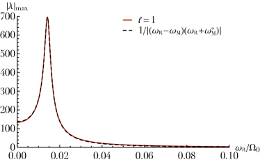
Figure 1: Illustration of the maximum eigenvalue norm, ${|\lambda(\omega_{\mathrm{R}})|_{\max}}$ of the susceptibility matrix ${\mathbf{N}_{\ell}(\omega_{\mathrm{R}})}$ for ${\ell\!=\!1}$, as a function of the real frequency ${\omega_{\mathrm{R}}/\Omega_{0}}$, with $\Omega_{0}$ the isochrone cluster’s frequency scale (see §C). One notes a clear amplification for frequencies close to the real part of the damped mode’s complex frequency, ${\omega_{\mathrm{R}}\!\simeq\!\mathrm{Re}[\omega_{\mathrm{M}}]}$. This amplification is well reproduced by a function ${\!\propto\!1/|(\omega_{\mathrm{R}}\!-\!\omega_{\mathrm{M}})(\omega_{\mathrm{R}}\!+\!\omega_{\mathrm{M}}^{*})|}$ that captures the effect from both damped modes with positive and negative real frequency. Here, we used the value of $\omega_{\mathrm{M}}$ inferred from Fig. 2, and only adjusted the function’s maximum height. See §C for the numerical details.

In that figure, we clearly observe a narrow amplification in frequency. This is the direct imprint along the real frequency line of the cluster’s nearby ${\ell\!=\!1}$ damped mode. Following Eq. (139) of Nelson & Tremaine (1999), it is natural to approximate this narrow amplification with

$$|\lambda(\omega_{\mathrm{R}})|_{\max}\propto\frac{1}{|(\omega_{\mathrm{R}}-\omega_{\mathrm{M}})(\omega_{\mathrm{R}}+\omega_{\mathrm{M}}^{*})|},$$ (18)

where $\omega_{\mathrm{M}}$ is the complex frequency of the damped mode (with ${\mathrm{Re}[\omega_{\mathrm{M}}]\!>\!0}$ and ${\mathrm{Im}[\omega_{\mathrm{M}}]\!<\!0}$). In Eq. (18), we also accounted for the contribution from the associated counter-rotating damped mode, ${-\omega_{\mathrm{M}}^{*}}$, whose existence is guaranteed by the cluster’s spherical invariance. In Fig. 1, we note in particular the good agreement between the approximation from Eq. (18) and the numerically measured maximum amplification eigenvalue.

Owing to our explicit analytic continuation of the response matrix in Eq. (14), we may push further this analysis by explicitly evaluating the cluster’s response matrix in the lower half of the complex plane, i.e. for ${\mathrm{Im}[\omega]\!<\!0}$. As such, we define the (complex) dispersion function

$$\varepsilon_{\ell}(\omega)=\det\big{[}\mathbf{I}-\mathbf{M}_{\ell}(\omega)\big{]},$$ (19)

so that damped mode corresponds to solutions of ${\varepsilon_{\ell}(\omega_{\mathrm{M}})\!=\!0}$ with ${\mathrm{Im}[\omega_{\mathrm{M}}]\!<\!0}$.

In Fig. 2, we present this dispersion function in the lower half of the complex frequency plane.

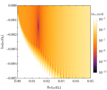
Figure 2: Illustration of the ${\ell\!=\!1}$ dispersion function ${\varepsilon_{\ell}(\omega)}$ in the lower half of the complex plane for the isotropic isochrone cluster. One clearly recovers the presence of a (weakly) damped mode of complex frequency ${\omega_{\mathrm{M}}/\Omega_{0}\!\simeq\!0.0143-0.00142\,\mathrm{i}}$. Further down in the complex plane, the present method saturates and suffers from spurious numerical oscillations.

From that figure, we infer that the isotropic isochrone cluster sustains a ${\ell\!=\!1}$ weakly damped mode of complex frequency

$$\omega_{\mathrm{M}}/\Omega_{0}\simeq 0.0143-0.00142\,\mathrm{i},$$ (20)

with ${\Omega_{0}\!=\!\sqrt{GM/b_{\mathrm{c}}^{3}}}$ the frequency scale of the isochrone cluster. We also recall that owing to spherical symmetry, there exists an associated damped mode of complex frequency ${-\omega_{\mathrm{M}}^{*}}$. We note that the present method suffers unfortunately from spurious numerical oscillations, as visible in Fig. 2, stemming from the Legendre series truncation.

As already pointed out by Weinberg (1994), this damped mode, as characterised by Eq. (20), is both (i) slow since ${\mathrm{Re}[\omega_{\mathrm{M}}]\!\ll\!\Omega_{0}}$, and (ii) weakly damped since ${|\mathrm{Im}[\omega_{\mathrm{M}}]/\mathrm{Re}[\omega_{\mathrm{M}}]|\!\ll\!1}$. These two properties are directly connected since the fact that ${\mathrm{Re}[\omega_{\mathrm{M}}]\!\ll\!\Omega_{0}}$ implies that only a small number of stars can effectively resonate with the mode (there are only a few slowly orbiting stars), which in turn only allows for an inefficient (Landau) damping of the mode itself.

Having determined the mode’s complex frequency, it is straightforward to obtain the mode’s radial dependence. (see, e.g., Eq. (72) of Hamilton et al. (2018)), as illustrated in Fig. 3.

Figure 3: Illustration of the density shape of the ${\ell\!=\!1}$ damped mode from Fig. 2. Top panel: Radial dependence of mode’s density, ${\rho(r)}$, and potential, ${\psi(r)}$. The normalisation of the vertical axis is arbitrary. Bottom panel: Illustration of the ${\ell\!=\!m\!=\!1}$ mode’s density in the ${(x,y)}$-plane. Overdensities (resp. underdensities) are shown in solid (reps. dashed) lines, spaced linearly between 95% and 5% of the maximum.

In that same figure, we also represent the shape of the associated ${\ell\!=\!m\!=\!1}$ density perturbation in the ${(x,y)}$-plane. We note in particular the striking similarity with the ${\ell\!=\!1}$ damped mode already presented in Fig. 4 of Weinberg (1994), in the context of the King sphere (a cluster with a finite radial extension) and recovered numerically in Fig. 6 of Heggie et al. (2020).

When excited, this ${\ell\!=\!1}$ mode manifests itself as dipole perturbation. This leads to a shift of the cluster’s density centre, as illustrated in Fig. 4.

Figure 4: Illustration of the overall effect of the density perturbation from Fig. 3 in solid lines, with contours spaced linearly between 95% and 5% of the background maximum. The maximum amplitude of the perturbation is fixed to 20% of the background maximum. The dashed contours correspond to the unperturbed cluster at the same levels. As already noted in Fig. 5 of Weinberg (1994), this perturbation leads to a shift of the cluster’s centre.

Once again, we emphasise the similarity with Fig. 5 of Weinberg (1994). All in all, this drives a sloshing motion of the cluster’s centre of typical frequency ${\mathrm{Re}[\omega_{\mathrm{M}}]}$, which, in the absence of any spontaneous emission, damps on a timescale set by ${\mathrm{Im}[\omega_{\mathrm{M}}]}$.

While in Fig. 2 we focused our interest on ${\ell\!=\!1}$ perturbations, we applied the same method for the other harmonics, namely ${\ell\!=\!0,2,3}$. We could not recover any significant damped mode before falling in the region of spurious numerical modes (as already visible in Fig. 2). Future works should focus on improving the present scheme’s numerical stability in order to delay the appearance of these artificial modes, as one explores the lower half of the complex plane further down.

Having characterised in detail the properties of the cluster’s ${\ell\!=\!1}$ damped mode, we finally set out to recover its imprints in direct $N$-body simulations. We follow an approach similar to the one presented in Spurzem & Aarseth (1996); Heggie et al. (2020), and we spell out details in §F.

We performed direct $N$-body simulations of ${N\!=\!10^{5}}$ isotropic isochrone clusters using NBODY6++GPU (Wang et al., 2015), keeping track of the stochastic wandering of the cluster’s density centre (Casertano & Hut, 1985), as illustrated in Fig. 5 (solid lines).

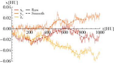
Figure 5: Illustration of one realisation of the random walk of the density centre as measured in one $N$-body realisation, in Hénon units ($\mathrm{HU}$; Hénon 1971). The dashed lines correspond to the filtered stochastic walks, see §F. The oscillations away from these smooth lines are notably signatures from the cluster’s damped ${\ell\!=\!1}$ mode.

In order not to be polluted by contributions from the outermost bound stars (see §F), we filter these time series (dashed lines) using a Savitzky–Golay (SG) filter on a timescale longer than the mode’s expected period. The oscillations of the time series around their underlying smooth evolutions are expected to be driven in part by the cluster’s damped mode.

To proceed further, similarly to Heggie et al. (2020), we finally estimate the power spectrum, ${P_{\mathrm{c}}(\omega)}$, of the distance of the cluster’s density centre w.r.t. its smooth evolution – see Eq. (72) for a detailed definition. Similarly to Eq. (18), we expect that for a real frequency $\omega_{\mathrm{R}}$ close to ${\mathrm{Re}[\omega_{\mathrm{M}}]}$, the power spectrum of the density centre should behave like a Lorentzian of the form

$$P_{\mathrm{c}}(\omega_{\mathrm{R}})\propto\frac{1}{|(\omega_{\mathrm{R}}\!-\!\omega_{\mathrm{M}})(\omega_{\mathrm{R}}\!+\!\omega_{\mathrm{M}}^{*})|^{2}},$$ (21)

where the value of the complex frequency $\omega_{\mathrm{M}}$ was obtained in Eq. (20). In that expression, similarly to Fig. 1, we accounted for the contributions from both damped modes, i.e. $\omega_{\mathrm{M}}$ and ${-\omega_{\mathrm{M}}^{*}}$, that only differ in the sign of their real part.

In Fig. 6, we present the estimation of ${P_{\mathrm{c}}(\omega)}$ along with its approximation from Eq. (21).

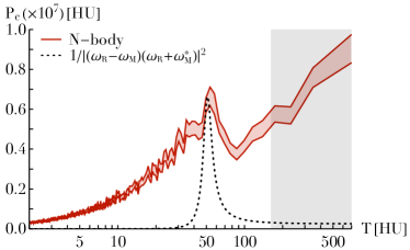
Figure 6: Illustration of the power spectrum, ${P_{\mathrm{c}}(T)}$, of the random motion of the cluster’s density centre, as measured in $N$-body simulations (solid lines), as a function of the period ${T\!=\!2\pi/\omega_{\mathrm{R}}}$ in Hénon units (${\mathrm{HU}}$). Errors are estimated through bootstrap resamplings over the available realisations, and the 16% and 84% confidence levels are represented. The dashed line corresponds to the prediction from Eq. (21), where only the overall amplitude has been adjusted to the one of the numerically measured peak. The gray region corresponds to the ${3\,\mathrm{dB}}$ cut region of the SG filter, so that it should not be considered. See §F for all the numerical details.

Reassuringly, we indeed recover the presence of a narrow amplification peak in the $N$-body simulations compatible with the one of the ${\ell\!=\!1}$ damped mode predicted using linear response theory. However, the measured peak seems slightly offset and somewhat too wide compared to the linear theory prediction. We note that Heggie et al. (2020) (see Fig. 4 therein), using a comparable method in King models, also recovered $N$-body power spectrums with wider peaks compared to the linear theory’s prediction. Likely origins for this disagreement include: (i) an incomplete numerical convergence of the $N$-body simulations; (ii) non time-stationary signal pollution associated with the system’s initial thermalisation during which the potential fluctuations get dressed (see, e.g., §A in Rogister & Oberman (1968), §F in Fouvry & Bar-Or (2018) and Lau & Binney (2019)).

5 Conclusion

In this work, we have shown how the matrix method for self-gravitating systems can naturally be tailored to also compute the (Landau) damped modes of a stellar system. In order to be able to apply Landau’s prescription, we had to (i) ‘align’ the resonant denominator with one of the integration coordinate, and (ii) project the integrand on some explicit basis function whose analytic continuation is straightforward. We applied this generic method to the isotropic isochrone cluster to recover the presence of a low-frequency weakly damped ${\ell\!=\!1}$ mode, as already demonstrated by Weinberg (1994) almost three decades ago. We also emphasised how the present approach, because it explicitly separates the orbital dependences w.r.t. the frequency ones (see Eq. (14)) offers a very efficient numerical scheme. Finally, following Heggie et al. (2020), we used direct $N$-body simulations to recover the main properties of this damped mode through the correlated stochastic motion of the clusters’ density centre. To conclude this work, we now mention a few possible venues for future works.

For the sake of simplicity, we limited ourselves to the sole consideration of an isotropic DF, ${F_{\mathrm{tot}}\!=\!F_{\mathrm{tot}}(E)}$, with an isochrone potential. Of course, it would be worthwhile to perform the same investigation for other classes of potentials, such as King spheres (Weinberg, 1994; Heggie et al., 2020). We note that applying the current method to cuspy profiles, e.g., Hernquist, would require some additional tuning, since the orbital frequencies, e.g., $\alpha$ as in Eq. (6), can diverge in the central regions. Similarly, following, e.g., Tremaine (2005), the present method would also require some further work to be applicable in dynamically degenerate systems such as quasi-Keplerian ones. Finally, lifting the assumption of velocity isotropy, i.e. considering ${F_{\mathrm{tot}}\!=\!F_{\mathrm{tot}}(E,L)}$, might offer new clues on the numerically observed accelerated relaxation of tangentially anisotropic clusters (Breen et al., 2017), the impact of rotation on a cluster’s long-term evolution (Rozier et al., 2019; Szölgyén et al., 2019; Breen et al., 2021) or its ${\ell\!=\!2}$ modes.

We also note that our use of the explicitly integrable isochrone potential eased the numerical tasks of various steps of the present application: (i) to perform systematically numerically stable orbit averages as in Eq. (24); (ii) to perform explicitly the change of coordinates towards the orbital frequencies as in Eq. (8); (iii) to determine the range of integrations ${v_{\mathbf{n}}^{-}(u)}$ and ${v_{\mathbf{n}}^{+}(u)}$ in Eq. (10); (iv) to easily determine the frequency range probed by every resonance vector $\mathbf{n}$, through ${\varpi_{\mathbf{n}}(\omega)}$ in Eq. (11). The present method should be extended to any arbitrary numerically-given radial potential, along with an appropriately tailored basis expansion (Weinberg, 1999). Such a generalisation is a necessary first step to ultimately hope for the explicit time integration of dressed kinetic equations such as the Balescu–Lenard equation (e.g., Fouvry et al., 2021).

Lau & Binney (2021) recently derived for the first time the van Kampen modes (Van Kampen, 1955) of isotropic stellar clusters, emphasising in particular how they allow for the detailed characterisation of the time-stationary thermal fluctuations present in a stellar cluster. Following the line of Case (1959), it will be undoubtedly be of interest to fully clarify the connexion between these genuine modes and the present damped ones.

Hamilton & Heinemann (2020) recently introduced the quasilinear collision operator in the context of stellar systems, to describe the evolution of the cluster’s distribution function as a result of resonant interactions with Landau damped waves. Benefiting from the present characterisation of a cluster’s ${\ell\!=\!1}$ damped mode, one should quantitatively investigate the heating signatures arising from such wave-particle interactions. In particular, noting that the present ${\ell\!=\!1}$ damped mode is low-frequency, so that resonant interactions with the mode only occur for very small orbital frequencies, it is expected that this process will only affect the cluster’s outskirts (see, e.g., Theuns, 1996), e.g., through the rate of stellar escapers (Hénon, 1960).

Finally, we focused here our interest on spherical stellar clusters. Without much work, the present method could also be applied to razor-thin axisymmetric stellar discs, since their action space is also ${2D}$. In particular, it would surely be physically enlightening to re-interpret the strong swing amplification that inevitably occurs in sufficiently self-gravitating stellar discs (see, e.g., Binney, 2020, and references therein) as the imprint of (weakly) damped modes.

Data Distribution

The code and the data underlying this article is available through reasonable request to the authors.

Appendix A Linear response theory in spherical systems

In this Appendix, we reproduce the key equations giving the response matrix of spherically symmetric stellar clusters. For a spherically symmetric system, the different spherical harmonics, $\ell$, decouple from one another. Following Eq. (B9) of Fouvry et al. (2021), the function ${G_{pq}^{\ell\mathbf{n}}(\mathbf{J})}$ introduced in Eq. (3) reads

$$G_{pq}^{\ell\mathbf{n}}(\mathbf{J})=-\frac{2(2\pi)^{3}}{2\ell+1}\big{|}y_{\ell}^{n_{2}}\big{|}^{2}\,L\,\mathbf{n}\!\cdot\!\frac{\partial F_{\mathrm{tot}}}{\partial\mathbf{J}}\,W_{\ell p}^{\mathbf{n}}(\mathbf{J})\,W_{\ell q}^{\mathbf{n}}(\mathbf{J}),$$ (22)

where we introduced ${y_{\ell}^{n}\!=\!Y_{\ell}^{n}(\tfrac{\pi}{2},0)}$, with ${Y_{\ell}^{m}(\vartheta,\phi)}$ the spherical harmonics normalised so that ${\!\int\!\mathrm{d}\vartheta\mathrm{d}\phi\sin(\vartheta)|Y_{\ell}^{m}(\vartheta,\phi)|^{2}\!=\!1}$. We note that these coefficients impose the constraints ${|n_{2}|\!\leq\!\ell}$ and ${(\ell\!-\!n_{2})}$ even, and that the vector ${\mathbf{n}\!=\!(0,0)}$ does not contribute to the response matrix. We also recall that the shape of an orbit is fully characterised by the action ${\mathbf{J}\!=\!(J_{r},L)}$, with $J_{r}$ the radial action, and $L$ the angular momentum, with the associated orbital frequencies ${\mathbf{\Omega}\!=\!(\Omega_{1},\Omega_{2})}$. Equation (22) also involves the system’s total DF, ${F_{\mathrm{tot}}(\mathbf{J})}$, normalised so that ${\!\int\!\mathrm{d}\mathbf{r}\mathrm{d}\mathbf{v}\,F_{\mathrm{tot}}\!=\!M}$ with $M$ the cluster’s total mass, and ${(\mathbf{r},\mathbf{v})}$ the position and velocity coordinates.

In Eq. (22), ${p,q\!\geq\!1}$ stand for the radial indices of the considered biorthogonal basis of potentials and densities. These are introduced following Kalnajs (1976), using the same convention as in Eq. (B1) of Fouvry et al. (2021). In practice, owing to spherical symmetry, it is natural to expand the potential basis elements as

$$\psi^{(\alpha)}(\mathbf{r})=Y_{\ell}^{m}(\vartheta,\phi)\,U_{n}^{\ell}(r),$$ (23)

and similarly for the densities, with ${U_{n}^{\ell}(r)}$ some real radial functions with ${n\!\geq\!1}$. In practice, we used radial basis elements from Clutton-Brock (1973), and we refer to §B1 of Fouvry et al. (2021) for an explicit expression of ${U_{n}^{\ell}(r)}$. Equation (22) also involves the coefficients

$$W_{\ell n}^{\mathbf{n}}(\mathbf{J})=\!\!\int_{0}^{\pi}\!\!\frac{\mathrm{d}\theta_{1}}{\pi}\,U_{n}^{\ell}(r)\,\cos(n_{1}\theta_{1}+n_{2}(\theta_{2}\!-\!\varphi)),$$ (24)

which correspond to the Fourier transform of the basis elements w.r.t. the canonical angles ${\bm{\theta}\!=\!(\theta_{1},\theta_{2}\!-\!\varphi)}$. Following Tremaine & Weinberg (1984) (recalled in §A of Fouvry et al. (2021)), they read

$$\theta_{1}=\!\!\int_{\mathcal{C}}\!\!\mathrm{d}r\,\frac{\Omega_{1}}{|v_{r}|};\quad\theta_{2}-\varphi{} =\!\!\int_{\mathcal{C}}\!\!\mathrm{d}r\,\frac{\Omega_{2}-L/r^{2}}{|v_{r}|},$$ (25)

with the radial velocity ${v_{r}^{2}\!=\!2(E\!-\!\psi(r))\!-\!L^{2}/r^{2}}$ and $\mathcal{C}$ the contour going from the orbit’s pericentre $r_{\mathrm{p}}$ up to the current position ${r\!=\!r(\theta_{1})}$ along the radial oscillation. Similarly, ${(\alpha,\beta)}$ from Eq. (6) are generically given by

$$\frac{1}{\alpha}=\frac{1}{\pi}\!\!\int_{r_{\mathrm{p}}}^{r_{\mathrm{a}}}\!\!\!\!\mathrm{d}r\,\frac{\Omega_{0}}{|v_{r}|};\quad\beta=\frac{1}{\pi}\!\!\int_{r_{\mathrm{p}}}^{r_{\mathrm{a}}}\!\!\!\!\mathrm{d}r\,\frac{L/r^{2}}{|v_{r}|},$$ (26)

with $r_{\mathrm{a}}$ the orbit’s apocentre. We refer to §B3 of Fouvry et al. (2021) for details regarding the computation of ${W_{\ell n}^{\mathbf{n}}(\mathbf{J})}$. These coefficients are the numerically most demanding quantities. We finally emphasise that our use of the isochrone potential allows for straightforward numerically stable angular averages, as highlighted in Eq. (G10) of Fouvry et al. (2021).

Appendix B Mapping to orbital frequencies

In this Appendix, we detail the change of variables ${(\alpha,\beta)\!\mapsto\!(u,v)}$ used to obtain Eq. (10).

From Eq. (9), we recall that the resonance frequency, ${\omega_{\mathbf{n}}(\alpha,\beta)}$, is defined as

$$\omega_{\mathbf{n}}(\alpha,\beta)=n_{1}\,\alpha+n_{2}\,\alpha\,\beta.$$ (27)

For a given $\mathbf{n}$, we define the minimum value reached by ${\omega_{\mathbf{n}}}$ as

$$\omega_{\mathbf{n}}^{\min}\!=\!\mathrm{Min}_{(\alpha,\beta)}[\omega_{\mathbf{n}}(\alpha,\beta)],$$ (28)

and similarly for $\omega_{\mathbf{n}}^{\max}$, recalling that ${(\alpha,\beta)}$ are confined to the domain from Eq. (7). We detail in §C how $\omega_{\mathbf{n}}^{\min}$ and $\omega_{\mathbf{n}}^{\max}$ can easily be determined in the case of the isochrone potential.

We then define the variable $u$ as

$$u=\frac{2\,\omega_{\mathbf{n}}(\alpha,\beta)-\omega_{\mathbf{n}}^{\max}-\omega_{\mathbf{n}}^{\min}}{\omega_{\mathbf{n}}^{\max}-\omega_{\mathbf{n}}^{\min}},$$ (29)

so that ${-1\!\leq\!u\!\leq\!1}$ by design. As for the second variable, $v$, we pick

$$v=\begin{cases}\displaystyle\beta&\text{if}\quad n_{2}=0,\\ \displaystyle\alpha&\text{if}\quad n_{2}\neq 0.\end{cases}$$ (30)

With such a choice, the Jacobian of the transformation ${(\alpha,\beta)\!\mapsto\!(u,v)}$ simply reads

$$\bigg{|}\frac{\partial(\alpha,\beta)}{\partial(u,v)}\bigg{|}=|\omega_{\mathbf{n}}^{\max}\!-\omega_{\mathbf{n}}^{\min}|\times\begin{cases}\displaystyle 1/|2n_{1}|&\text{if}\quad n_{2}=0,\\[8.61108pt] \displaystyle 1/|2n_{2}v|&\text{if}\quad n_{2}\neq 0,\end{cases}$$ (31)

where we recall that ${\mathbf{n}\!=\!(n_{1},n_{2})\!=\!(0,0)}$ does not contribute to the response matrix. All in all, this allows us to obtain the expression of ${G_{\mathbf{n}}(u,v)}$ from Eq. (10) as

$$G_{\mathbf{n}}(u,v)=\frac{2}{\omega_{\mathbf{n}}^{\max}\!-\omega_{\mathbf{n}}^{\min}}\,\bigg{|}\frac{\partial(\alpha,\beta)}{\partial(u,v)}\bigg{|}\,G_{\mathbf{n}}(\alpha,\beta),$$ (32)

with ${G_{\mathbf{n}}(\alpha,\beta)}$ introduced in Eq. (8).

Let us now detail how the minimum and maximum frequencies, ${(\omega_{\mathbf{n}}^{\min},\omega_{\mathbf{n}}^{\max})}$, may be determined. We note that ${\partial\omega_{\mathbf{n}}/\partial\alpha}$ (resp. ${\partial\omega_{\mathbf{n}}/\partial\beta}$) is of constant sign for fixed $\beta$ (resp. fixed $\alpha$). As a consequence, following Eq. (7), the extrema of $\omega_{\mathbf{n}}$ are reached either in the three edges ${(0,\tfrac{1}{2})}$, ${(0,1)}$, ${(1,\tfrac{1}{2})}$, or along the curve ${(\alpha,\beta_{\mathrm{c}}(\alpha))}$ with ${0\!\leq\!\alpha\!\leq\!1}$. This greatly simplifies the search of these extremum values, as one is left with investigating the behaviour of the function

$$\omega_{\mathbf{n}}^{\mathrm{c}}(\alpha)=n_{1}\,\alpha+n_{2}\,\alpha\,\beta_{\mathrm{c}}(\alpha).$$ (33)

We detail this characterisation in §C for the isochrone potential.

In addition to determining ${(\omega_{\mathbf{n}}^{\min},\omega_{\mathbf{n}}^{\max})}$, Eq. (10) also requires the knowledge of the integration boundaries ${(v_{\mathbf{n}}^{-}(u),v_{\mathbf{n}}^{+}(u))}$. Following Eq. (29), we first introduce the quantity

$$h_{\mathbf{n}}(u)=\tfrac{1}{2}\big{[}\omega_{\mathbf{n}}^{\max}\!+\omega_{\mathbf{n}}^{\min}+u(\omega_{\mathbf{n}}^{\max}\!-\omega_{\mathbf{n}}^{\min})\big{]}.$$ (34)

For ${n_{2}\!=\!0}$, Eq. (30) then gives the simple bounds

$$v_{\mathbf{n}}^{-}(u)=\tfrac{1}{2};\quad v_{\mathbf{n}}^{+}(u)=\beta_{\mathrm{c}}(h_{\mathbf{n}}(u)/n_{1}).$$ (35)

For ${n_{2}\!\neq\!0}$, the integration bounds are more intricate to determine. Following the mapping from Eq. (30) and the allowed domain from Eq. (7), $v$ must satisfy the four constraints

$$0\!\leq\!v;\;\;v\!\leq\!1;\;\;\frac{1}{2}\!\leq\!\frac{h_{\mathbf{n}}(u)}{n_{2}v}-\frac{n_{1}}{n_{2}};\;\;\frac{h_{\mathbf{n}}(u)}{n_{2}v}-\frac{n_{1}}{n_{2}}\!\leq\!\beta_{\mathrm{c}}(v).$$ (36)

The first two constraints are straightforward to account for. The third one is also easily incorporated provided one deals carefully with the respective signs of $n_{2}$ and ${n_{1}\!+\!\tfrac{1}{2}n_{2}}$. For ${n_{2}\!>\!0}$, the fourth and final constraint can be rewritten as ${h_{\mathbf{n}}(u)\!\leq\!\omega_{\mathbf{n}}^{\mathrm{c}}(v)}$, with the opposite inequality for ${n_{2}\!<\!0}$. As a consequence, getting the bounds associated with this constraint asks for the computation of the root of the function ${v\!\mapsto\!h_{\mathbf{n}}(u)\!-\!\omega_{\mathbf{n}}^{\mathrm{c}}(v)}$, at most twice. Fortunately, for the isochrone potential (see §C), the function ${\omega_{\mathbf{n}}^{\mathrm{c}}(v)}$ is explicitly known, and its extrema as well. In practice, once appropriate bracketing intervals are found, we used the bisection method to find the required roots. Accounting simultaneously for all these constraints finally provide us with the values of ${(v_{\mathbf{n}}^{-}(u),v_{\mathbf{n}}^{+}(u))}$ appearing in Eq. (10). Finally, for a given value of $u$, once ${(v_{\mathbf{n}}^{-}(u),v_{\mathbf{n}}^{+}(u))}$ determined, we compute the integral over ${\mathrm{d}v}$ in Eq. (10) using a midpoint rule with $K_{v}$ nodes.

Appendix C Isochrone potential

In this Appendix, we detail key expressions of the isochrone potential (Hénon, 1959), following notations similar to §G of Fouvry et al. (2021). We emphasise that the availability of these various analytical expressions greatly eased the practical implementation of the method described in the main text.

The isochrone potential is defined as

$$\psi(r)=-\frac{GM}{b_{\mathrm{c}}+\sqrt{b_{\mathrm{c}}^{2}+r^{2}}},$$ (37)

with $b_{\mathrm{c}}$ the associated lengthscale. In that case, the frequency scale from Eq. (5) takes the simple form

$$\Omega_{0}=\sqrt{\frac{GM}{b_{\mathrm{c}}^{3}}}.$$ (38)

As defined in Eq. (6), the dimensionless radial frequency, $\alpha$, and the frequency ratio, $\beta$, take the simple form

$$\alpha=\bigg{(}\frac{2E}{E_{0}}\bigg{)}^{3/2};\quad\beta=\tfrac{1}{2}\bigg{(}1+\frac{L}{\sqrt{L^{2}+4L_{0}^{2}}}\bigg{)},$$ (39)

with the energy and action scales, ${E_{0}\!=\!-GM/b_{\mathrm{c}}}$ and ${L_{0}\!=\!\sqrt{GMb_{\mathrm{c}}}}$. Fortunately, Eq. (39) can be readily inverted to determine the energy and angular momentum of an orbit with given frequencies. One simply has

$$E=\tfrac{1}{2}E_{0}\,\alpha^{2/3};\quad L=L_{0}\,\frac{2\beta-1}{\sqrt{\beta(1-\beta)}}.$$ (40)

All in all, these mappings allow for the straightforward computation of the Jacobian ${|\partial\mathbf{J}/\partial(\alpha,\beta)|}$ appearing in Eq. (8), recalling that ${|\partial\mathbf{J}/\partial(E,L)|\!=\!1/\Omega_{1}}$.

As given in Eq. (G8) of Fouvry et al. (2021), along circular orbits, one has

$$\alpha_{\mathrm{c}}(x)=\bigg{(}\frac{1}{\sqrt{1+x^{2}}}\bigg{)}^{3/2};\quad\beta_{\mathrm{c}}(x)=\frac{\sqrt{1+x^{2}}}{1+\sqrt{1+x^{2}}},$$ (41)

with ${x\!=\!r/b_{\mathrm{c}}}$. Luckily, these two relations can easily be leveraged to express the frequency ratio, ${\beta_{\mathrm{c}}}$, along circular orbits, as a function of the associated (dimensionless) radial frequency. One gets

$$\beta_{\mathrm{c}}(\alpha)=\frac{1}{1+\alpha^{2/3}}.$$ (42)

It is this function that characterises the bound of the integration domain in Eq. (8).

Finally, for a given resonance $\mathbf{n}$, we must determine the minimum and maximum frequencies, ${(\omega_{\mathbf{n}}^{\min},\omega_{\mathbf{n}}^{\max})}$ as defined in Eq. (28). This asks for the determination of the extrema of the function ${\alpha\!\mapsto\!\omega_{\mathbf{n}}^{\mathrm{c}}(\alpha)}$, as defined in Eq. (33). Owing to Eq. (42), for the isochrone potential one has

$$\frac{\partial\omega_{\mathbf{n}}^{\mathrm{c}}}{\partial\alpha}=\frac{P_{\mathbf{n}}(q)}{3q^{2}},$$ (43)

with ${q\!=\!1\!+\!\alpha^{2/3}}$. In Eq. (43), we also introduced the polynomial

$$P_{\mathbf{n}}(q)=3n_{1}q^{2}+n_{2}q+2n_{2}.$$ (44)

Given that ${P(q)}$ is at most a second-order polynomial, it is straightforward to determine the existence/absence of extrema for the function ${\alpha\!\mapsto\!\omega_{\mathbf{n}}^{\mathrm{c}}(\alpha)}$. We also note that the same polynomial, ${P_{\mathbf{n}}(q)}$, is used to fully characterise the integration bounds ${(v_{\mathbf{n}}^{-}(u),v_{\mathbf{n}}^{+}(u))}$, as constrained by Eq. (36).

In order to validate our implementation of the response matrix, we recovered the radial-orbit instability in a radially anisotropic isochrone potential, as investigated in Saha (1991). We refer to §G of Fouvry et al. (2021) for the detailed definition of the considered DF. For this calculation, we used a total of ${n_{\mathrm{max}}\!=\!100}$ basis elements with the scale radius ${R_{\mathrm{b}}\!=\!20\,b_{\mathrm{c}}}$ (see §B1 in Fouvry et al. (2021)), and the sum over resonance number was truncated at ${n_{1}^{\max}\!=\!10}$. The orbit-averages in Eq. (24) were performed with ${K\!=\!200}$ steps, while the integrations w.r.t. $v$ (see Eq. (10)) were performed with ${K_{v}\!=\!200}$ steps, and the GL quadrature used ${K_{u}\!=\!200}$ nodes.

In Fig. 7, we recover that the radially-anisotropic model, ${R_{\mathrm{a}}\!=\!b_{\mathrm{c}}}$ supports an unstable mode with growth rate ${\eta\!\simeq\!0.023\,\Omega_{0}}$ in good agreement with the value ${0.024\,\Omega_{0}}$ obtained by Saha (1991).

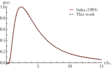
Figure 7: Illustration of the radial shape, ${\psi(r)}$, as presented in Fig. 4 of Saha (1991) and compared with the present method, for the ${\ell\!=\!2}$ unstable mode of a radially anisotropic ${R_{\mathrm{a}}\!=\!b_{\mathrm{c}}}$ isochrone cluster. The normalisation of the vertical axis is arbitrary. See the text for the detailed numerical parameters.

Similarly, the radial shapes of the modes are in good agreement. This strengthens our confidence in the present method, at least when searching for instabilities in the upper half of the complex frequency plane.

In §4, when investigating the cluster’s ${\ell\!=\!1}$ damped mode, we used the exact same numerical control parameters as in Fig. 7. In order to further assess the appropriate numerical convergence of the numerical scheme, following the same calculation as in Fig. 1, we present in Fig. 8 the maximum norm of the susceptibility matrix ${|N_{pq}^{\ell}(\omega_{\mathrm{R}})|}$ as one varies the real frequency $\omega_{\mathrm{R}}$, for ${\ell\!=\!1}$ and fixed ${(p,q)}$.

Figure 8: Illustration of the maximum norm, ${|N_{pq}^{\ell}|_{\max}}$, of the susceptibility matrix ${\mathbf{N}_{\ell}(\omega_{\mathrm{R}})\!=\![\mathbf{I}\!-\!\mathbf{M}_{\ell}(\omega_{\mathrm{R}})]^{-1}}$ for ${\ell\!=\!1}$, as one varies the real frequency $\omega_{\mathrm{R}}$ for fixed ${(p,q)}$. Values smaller than ${0.05}$ are replaced with white colors, highlighting the fact that ${N_{pq}\!\to\!\delta_{pq}}$ for ${p,q\!\gg\!1}$.

In that figure, we recover in particular that for ${p,q\!\gg\!1}$, one has ${N_{pq}(\omega_{\mathrm{R}})\!\to\!\delta_{pq}}$, i.e. collective effects can be safely neglected on small physical scales.

Appendix D Legendre functions

In this Appendix, we detail our use of the GL quadrature and our computation of the Legendre functions.

The Legendre polynomials satisfy the normalisation

$$\!\!\int_{-1}^{1}\!\!\mathrm{d}u\,P_{k}(u)\,P_{k^{\prime}}(u)=c_{k}\,\delta_{kk^{\prime}},$$ (45)

with ${c_{k}\!=\!2/(2k\!+\!1)}$. Following Eq. (13), a given coefficient $a_{k}$ is given by

$$a_{k}=\frac{1}{c_{k}}\!\!\int_{-1}^{1}\!\!\mathrm{d}u\,G(u)\,P_{k}(u).$$ (46)

In practice, these coefficients are directly computed through a GL quadrature of order $K_{u}$ (see, e.g., Press et al., 2007). As such, we have at our disposal an explicit set of nodes, ${\{u_{i}\}_{1\leq i\leq K_{u}}}$, and weights ${\{w_{i}\}_{1\leq i\leq K_{u}}}$. Then, for any ${0\!\leq\!k\!<\!K_{u}}$, one approximates the integral from Eq. (46) through

$$a_{k}=\frac{1}{c_{k}}\sum_{i=1}^{K_{u}}w_{i}\,G(u_{i})\,P_{k}(u_{i}),$$ (47)

noting that the values of ${\{P_{k}(u_{i})\}_{i,k}}$ may be computed once and for all, independently of the function ${G(u)}$.

In order to compute the response matrix, following Eq. (15), one has to evaluate the functions

$$D_{k}(\omega)=\!\!\int_{\begin{subarray}{c}\\[2.50153pt] -1\\ \mathcal{L}\end{subarray}}^{1}\!\!\mathrm{d}u\,\frac{P_{k}(u)}{u-\omega},$$ (48)

The ${P_{k}(u)}$ are analytic functions that can readily be evaluated in the whole complex plane. As such, applying Landau’s prescription from Eq. (2), we can rewrite Eq. (48) as

$$D_{k}(\omega)=\begin{cases}\displaystyle Q_{k}(\omega)&\!\!\!\text{if}\;\;\mathrm{Im}[\omega]>0,\\[8.61108pt] \displaystyle Q_{k}(\omega)\!+\!\mathrm{i}\pi P_{k}(\omega)\,H(\omega)&\!\!\!\text{if}\;\;\mathrm{Im}[\omega]=0,\\[8.61108pt] \displaystyle Q_{k}(\omega)\!+\!2\mathrm{i}\pi P_{k}(\omega)\,H(\mathrm{Re}[\omega])&\!\!\!\text{if}\;\;\mathrm{Im}[\omega]<0.\end{cases}$$ (49)

In that expression, we introduced the Heaviside function of the ${[-1,1]}$ interval, ${H(x)}$ with ${x\!\in\!\mathbb{R}}$, as

$$H(x)=\begin{cases}\displaystyle 0&\text{if}\quad x<-1,\\[4.30554pt] \displaystyle\tfrac{1}{2}&\text{if}\quad x=-1,\\[4.30554pt] \displaystyle 1&\text{if}\quad-1<x<1,\\[4.30554pt] \displaystyle\tfrac{1}{2}&\text{if}\quad x=1,\\[4.30554pt] \displaystyle 0&\text{if}\quad 1<x.\end{cases}$$ (50)

In Eq. (49), we also introduced the function ${Q_{k}(\omega)}$ defined as

$$Q_{k}(\omega)=\begin{cases}\displaystyle\!\!\int_{-1}^{1}\!\!\mathrm{d}u\,\frac{P_{k}(u)}{u-\omega}&\text{if}\quad\mathrm{Im}[\omega]>0,\\ \displaystyle\mathcal{P}\!\!\int_{-1}^{1}\!\!\mathrm{d}u\,\frac{P_{k}(u)}{u-\omega}&\text{if}\quad\mathrm{Im}[\omega]=0,\\ \displaystyle\!\!\int_{-1}^{1}\!\!\mathrm{d}u\,\frac{P_{k}(u)}{u-\omega}&\text{if}\quad\mathrm{Im}[\omega]<0.\end{cases}$$ (51)

The Legendre polynomials, ${P_{k}(\omega)}$, generically satisfy Bonnet’s recursion formula. For ${k\!\geq\!1}$, it reads

$$(k+1)\,P_{k+1}(\omega)=(2k+1)\,\omega\,P_{k}(\omega)-k\,P_{k-1}(\omega).$$ (52)

Given the definition from Eq. (51), the exact same recurrence relation also applies for ${Q_{k}(\omega)}$. It now only remains to specify the initial conditions of these functions. For the Legendre polynomials, one naturally has

$$P_{0}(\omega)=1;\quad P_{1}(\omega)=\omega.$$ (53)

For the function ${Q_{0}(\omega)}$, we straightforwardly obtain the expression

$$Q_{0}(\omega)=\begin{cases}\displaystyle\ln(1\!-\!\omega)-\ln(-1\!-\!\omega)&\text{if}\quad\mathrm{Im}[\omega]>0,\\[8.61108pt] \displaystyle\ln(|1\!-\!\omega|)-\ln(|-1\!-\!\omega|)&\text{if}\quad\mathrm{Im}[\omega]=0,\\[8.61108pt] \displaystyle\ln(1\!-\!\omega)-\ln(-1\!-\!\omega)&\text{if}\quad\mathrm{Im}[\omega]<0,\end{cases}$$ (54)

where the complex logarithm, ${\ln(\omega)}$, is defined with its usual branch cut in ${\mathrm{Im}[\omega]=0}$ and ${\mathrm{Re}[\omega]<0}$. Finally, noting that

$$\frac{P_{1}(u)}{u-\omega}=\frac{u}{u-\omega}=1+\frac{\omega}{u-\omega}=1+\omega\,\frac{P_{0}(u)}{u-\omega},$$ (55)

we can complement Eq. (54) with the additional relation

$$Q_{1}(\omega)=2+\omega\,Q_{0}(\omega).$$ (56)

In Fig. 9, we illustrate the behaviour of the function ${D_{0}(\omega)}$.

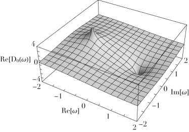
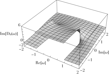
Figure 9: Illustration of the complex function ${D_{0}(\omega)}$ as defined in Eq. (48). The top panel corresponds to ${\mathrm{Re}[D_{0}(\omega)]}$, and the bottom one to ${\mathrm{Im}[D_{0}(\omega)]}$. As expected, this function does not suffer from any discontinuities in the upper half of the complex plane, i.e. in the region of unstable modes.

We note that this function does not present any discontinuities in the upper half of the complex plane, but suffers from two discontinuities in the lower half, namely: (i) ${\mathrm{Re}[D_{0}(\omega)]}$ diverges in ${\omega\!=\!\pm 1}$; (ii) ${\mathrm{Im}[D_{0}(\omega)]}$ has step discontinuities along all the lines ${\mathrm{Im}[\omega]\!<\!0}$, in the locations ${\mathrm{Re}[\omega]\!=\!\pm 1}$. Such discontinuities originate from the fact that the integral from Eq. (48) only covers a finite range of frequencies, i.e. ${-1\!\leq\!u\!\leq\!1}$.

For a given value of $K_{u}$ and a given complex frequency $\omega$, a natural way to compute ${\{P_{k}(\omega)\}_{0\leq k<K_{u}}}$ and ${\{Q_{k}(\omega)\}_{0\leq k<K_{u}}}$ is to use Eq. (52) as a forward recurrence relation. Namely, one starts from the initial conditions given by Eqs. (53), (54) and (56), and, for ${k\!\geq\!2}$, uses the recurrence relation

$$P_{k}(\omega)=\frac{2k-1}{k}\,\omega\,P_{k-1}(\omega)-\frac{k-1}{k}\,P_{k-2}(\omega),$$ (57)

similarly for ${Q_{k}(\omega)}$.

Yet, for some values of $\omega$ such a recurrence relation is not numerically stable to compute ${Q_{k}(\omega)}$. In that case, we may resort to a backward recurrence. To do so, we give ourselves a ‘warm-up’ starting point, ${K_{\mathrm{c}}\!>\!K_{u}}$, and initialise the recurrence with

$$Q_{K_{\mathrm{c}}+2}(\omega)=0;\quad Q_{K_{\mathrm{c}}+1}(\omega)=1.$$ (58)

Such an initial condition is appropriate because when the forward recurrence is unstable it is because one is interested in the decaying mode of recurrence, which, fortunately, becomes the growing one of the backward recurrence (see, e.g., Zhang & Jin, 1996). In that case, the recurrence is propagated backwards using, for ${k\!\geq\!0}$, the relation

$$Q_{k}(\omega)=\frac{2k+3}{k+1}\,\omega\,Q_{k+1}(\omega)-\frac{k+2}{k+1}\,Q_{k+2}(\omega).$$ (59)

Once ${Q_{0}(\omega)}$ has been reached, owing to the linearity of Eq. (59), we rescale all the computed values ${\{Q_{k}(\omega)\}_{0\leq k<K_{u}}}$ to the correct value of ${Q_{0}(\omega)}$ given by Eq. (54).

For a given value of $\omega$ and $K_{u}$, it only remains to setup a criteria to specify whether the forward or backward recurrence relation should be used. In practice, we follow the exact same criteria as in Heiter (2010) (see in particular the function qtm1 therein). The Legendre functions, ${P_{k}(\omega)}$, are always computed with the forward recurrence relation from Eq. (57). For the functions ${Q_{k}(\omega)}$, we use the forward recurrence if $\omega$ lies within a given ellipse around the real segment ${-1\!\leq\!\mathrm{Re}[\omega]\!\leq\!1}$ and ${\mathrm{Im}[\omega]\!=\!0}$. More precisely, we define

$$b=\mathrm{Min}\bigg{[}1,\frac{4.5}{(K_{u}+1)^{1.17}}\bigg{]};\quad a=\sqrt{1+b^{2}}.$$ (60)

Then, if ever the criterion

$$\bigg{(}\frac{\mathrm{Re}[\omega]}{a}\bigg{)}^{2}+\bigg{(}\frac{\mathrm{Im}[\omega]}{b}\bigg{)}^{2}\leq 1$$ (61)

is satisfied, we use the forward recurrence from Eq. (57). When Eq. (61) is not satisfied, we resort to the backward recurrence from Eq. (59). In that case, the warm-up, $K_{\mathrm{c}}$ – see Eq. (58), is determined through

$$z{} =\big{|}\mathrm{Re}[\omega]\big{|}+\mathrm{i}\,\big{|}\mathrm{Im}[\omega]\big{|};\quad c=\sqrt{z^{2}-1};$$

$$d{} =2\,\ln(|z+c|);\quad K_{\mathrm{c}}=K_{u}+\bigg{\lceil}\frac{\ln(1/\epsilon)}{d}\bigg{\rceil},$$ (62)

with ${\epsilon\!=\!10^{-14}}$ a given tolerance target.

Appendix E Homogeneous stellar systems

In this Appendix, we apply the method from Eq. (14) to an homogeneous stellar system (see §5.2.4 of Binney & Tremaine, 2008). This is useful to test our implementation of the Legendre functions, as well as the numerical stability of the overall scheme. As such, we consider the simple case of a $1D$ Maxwellian velocity distribution with

$$M(\omega)=\frac{q}{\sqrt{\pi}}\!\!\int_{\begin{subarray}{c}\\[2.50153pt] -\infty\\ \mathcal{L}\end{subarray}}^{+\infty}\!\!\!\!\mathrm{d}u\,\frac{u\,\mathrm{e}^{-u^{2}}}{u-\omega}$$ (63)

where ${0\!<\!q\!<\!1}$ ensures linear stability. Following Eq. (5.64) of Binney & Tremaine (2008), one can rewrite Eq. (63) under the simple form

$$M(\omega)=q\big{(}1+\omega\,Z(\omega)\big{)},$$ (64)

with the usual plasma dispersion function (Fried & Conte, 1961)

$$Z(\omega)=\frac{1}{\sqrt{\pi}}\!\!\int_{\begin{subarray}{c}\\[2.50153pt] -\infty\\ \mathcal{L}\end{subarray}}^{+\infty}\!\!\!\!\mathrm{d}x\,\frac{\mathrm{e}^{-x^{2}}}{x-\omega},$$ (65)

which can readily be evaluated in the whole complex plane.

We then compare the analytical expression from Eq. (64) with the result obtained by applying the method from Eq. (14). To do so, we introduce a truncation velocity, ${u_{\mathrm{max}}\!>\!0}$, and rewrite Eq. (63) as

$$M(\omega)=\!\!\int_{\begin{subarray}{c}\\[2.50153pt] -1\\ \mathcal{L}\end{subarray}}^{1}\!\!\mathrm{d}u\,\frac{G(u)}{u-\varpi},$$ (66)

with

$$G(u)=\frac{q\,u_{\mathrm{max}}}{\sqrt{\pi}}\,u\,\mathrm{e}^{-u_{\mathrm{max}}^{2}u^{2}};\quad\varpi=\frac{\omega}{u_{\mathrm{max}}}.$$ (67)

Given that Eq. (12) and (66) are of the exact same form, we may use the same Legendre projection as in Eq. (14). In Fig. 10 we illustrate the contours of the associated dispersion function in the lower half of the complex frequency space.

Figure 10: Illustration of the contours of the dispersion function, ${\ln(|\varepsilon(\omega)|)\!=\!\ln(|1\!-\!M(\omega)|)}$ in the lower half of the complex plane for the (stable) homogeneous case from Eq. (63), with ${q\!=\!\tfrac{1}{2}}$. Around each pole, the outermost contours correspond to ${\ln(|\varepsilon|)\!=\!-0.5}$ with the subsequent contours spaced every ${-0.5}$. Top panel: Analytical prediction from Eq. (64) computed with ${u_{\mathrm{max}}\!=\!+\infty}$. Bottom panel: Numerical prediction from Eq. (66), truncating the velocity integral at ${u_{\mathrm{max}}\!=\!20}$ and using ${K_{u}\!=\!200}$ points to perform the GL quadrature.

We note that both methods are in very good agreement for the first few damped modes. For larger damping rates, the present numerical method produces spurious zeros, stemming from the Legendre series truncation – a problem also encountered in Fig. 2 of Weinberg (1994). Similar artificial zeros are also present in the self-gravitating case presented here in Fig. 2.

Appendix F Numerical simulations

In this Appendix, we detail the numerical simulations used in Figs. 5 and 6. The direct $N$-body simulations were performed with NBODY6++GPU (Wang et al., 2015) using a setup identical to the ones presented in Fouvry et al. (2021) (§H1 therein). Each simulation is composed of ${N\!=\!10^{5}}$ particles, integrated for a total duration ${t_{\mathrm{max}}\!=\!10^{3}\,\mathrm{HU}}$, with an output every ${\Delta t\!=\!1\,\mathrm{HU}}$. For the isochrone potential, Hénon units (Hénon, 1971) are such that ${G\!=\!M\!=\!R_{\mathrm{v}}}$, with $M$ the cluster’s total mass and ${R_{\mathrm{v}}\!=\!6\,b_{\mathrm{c}}/(3\pi\!-\!8)}$ the virial radius. We performed a total of ${N_{\mathrm{real}}\!=\!200}$ different realisations.

For each output, the position of the density centre was estimated using the algorithm from Casertano & Hut (1985) with ${j\!=\!6}$ neighbours. Once the position of the density centre estimated, we followed the same recentring as in Heggie et al. (2020). Namely, we place ourselves within the inertial frame moving along with the system’s barycentric uniform motion and fix the origin of the coordinate’s system so that all the density centres start their evolution from ${\mathbf{r}\!=\!\mathbf{0}}$. Following these manipulations, each realisation provides us with three time series, namely ${\{x_{\mathrm{c}}(t),y_{\mathrm{c}}(t),z_{\mathrm{c}}(t)\}}$.

The density of the isochrone cluster scales likes ${\rho(r)\!\propto\!1/r^{4}}$ for ${r\!\to\!+\infty}$. As such, it is a rather ‘puffy’ cluster, i.e. one with a significant population of very loosely bound stars. More precisely, following Eq. (2.51) of Binney & Tremaine (2008), the mass outside radius $r$ in the isochrone model is of order ${2b_{\mathrm{c}}M/r}$. As a consequence, the outermost bound star is at a radius of order ${2Nb_{\mathrm{c}}}$. While this outermost star orbits the system, it will drive significant excursions of the cluster’s density centre of typical lengths ${2\,b_{\mathrm{c}}\!\simeq\!0.5\,\mathrm{HU}}$, likely visible in Fig. 5 (D. Heggie, private communication). We also point out that the timescales associated with these oscillations is long, and cannot be directly resolved within the timespan of our simulations. In order not to be polluted by these contributions, one must therefore filter our time series to better single out the effect of the cluster’s damped mode on the correlated motion of the cluster’s density centre.

In that view, we followed an approach similar to Spurzem & Aarseth (1996). For a given realisation, each of the time series, ${\{x_{\mathrm{c}}(t),y_{\mathrm{c}}(t),z_{\mathrm{c}}(t)\}}$ is filtered using a SG filter (see, e.g., Schafer, 2011). Such a filter is characterised by a (half-)window size $M_{\mathrm{f}}$ and an order $N_{\mathrm{f}}$. In practice, in order not to affect the frequency associated with the damped mode, we used ${M_{\mathrm{f}}\!=\!153\!\simeq\!3\,T_{\mathrm{M}}/\Delta t}$, with the mode’s period ${T_{\mathrm{M}}\!=\!2\pi/\mathrm{Re}[\omega_{\mathrm{M}}]\!\simeq\!50.8\,\mathrm{HU}}$, as given by Eq. (20). We arbitrarily fixed the order of the filter to ${N_{\mathrm{f}}\!=\!5}$. For a given choice of filtering parameters, we can then estimate the ${3\,\mathrm{dB}}$ cutoff period of the filter, $T_{\mathrm{c}}$, through Eq. (12) of Schafer (2011). It reads here

$$T_{\mathrm{c}}\simeq\frac{2\,(3.2\,M_{\mathrm{f}}-4.6)}{N_{\mathrm{f}}+1}\,\Delta t\simeq 167\,\mathrm{HU}.$$ (68)

This cutoff period is such that any signal on period faster than $T_{\mathrm{c}}$ is essentially left untouched by the filtering, hence the requirement ${T_{\mathrm{c}}\!>\!T_{\mathrm{M}}}$ to characterise the mode’s properties.

Owing to this filtering, we construct the filtered time series

$$\delta x_{\mathrm{c}}(t)=x_{\mathrm{c}}(t)-\overline{x}_{\mathrm{c}}(t),$$ (69)

(similarly for $y_{\mathrm{c}}$ and $z_{\mathrm{c}}$) where ${\overline{x}_{\mathrm{c}}(t)}$ is obtained via the filtering of ${x_{\mathrm{c}}(t)}$ and is illustrated in Fig. 5. Following Spurzem & Aarseth (1996), for each realisation we finally construct one time series

$$\delta R_{\mathrm{c}}(t)=\sqrt{\big{[}\delta x_{\mathrm{c}}(t)\big{]}^{2}+\big{[}\delta y_{\mathrm{c}}(t)\big{]}^{2}+\big{[}\delta z_{\mathrm{c}}(t)\big{]}^{2}}.$$ (70)

Recalling that our effective sampling rate is ${\Delta t\!=\!1\,\mathrm{HU}}$, each time series consist then of an array ${\{\delta R_{i}\}_{0\leq i<n}}$, with ${n\!=\!1001\!-\!2M_{\mathrm{f}}}$ the total length of the available signal after the filtering. For ${0\!\leq\!k\!<\!n}$, we define the discrete Fourier transform with the convention

$$\widehat{\delta R}_{k}=\frac{1}{n}\sum_{i=0}^{n-1}\delta R_{i}\,\mathrm{e}^{-\mathrm{i}2\pi ik/n},$$ (71)

so that ${\widehat{\delta R}_{k}}$ is associated with the frequency ${\omega_{k}\!=\!\frac{2\pi k}{n}\tfrac{1}{\Delta t}}$. Finally, we construct the associated power spectrum

$$P_{\mathrm{c}}(\omega_{k})=\big{|}\widehat{\delta R}_{k}\big{|}^{2}.$$ (72)

This is the quantity presented in Fig. 6.

To finalise our measurement, Eq. (72) is ensemble-averaged over all the $N_{\mathrm{real}}$ realisations available. In order to estimate the associated errors, we performed ${N_{\mathrm{boot}}\!=\!N_{\mathrm{real}}}$ bootstrap resamplings over the available realisations. This is presented in Fig. 6 with the associated ${16\%}$ and ${84\%}$ error levels.

References

- Binney (2020) Binney J., 2020, MNRAS, 496, 767
- Binney & Tremaine (2008) Binney J., Tremaine S., 2008, Galactic Dynamics: Second Edition. Princeton Univ. Press
- Breen et al. (2017) Breen P. G., Varri A. L., Heggie D. C., 2017, MNRAS, 471, 2778
- Breen et al. (2021) Breen P. G., Rozier S., Heggie D. C., Varri A. L., 2021, MNRAS, 502, 4762
- Case (1959) Case K. M., 1959, Ann. Phys., 7, 349
- Casertano & Hut (1985) Casertano S., Hut P., 1985, ApJ, 298, 80
- Clutton-Brock (1973) Clutton-Brock M., 1973, Ap&SS, 23, 55
- Fouvry & Bar-Or (2018) Fouvry J.-B., Bar-Or B., 2018, MNRAS, 481, 4566
- Fouvry et al. (2021) Fouvry J.-B., Hamilton C., Rozier S., Pichon C., 2021, MNRAS, submitted
- Fried & Conte (1961) Fried B. D., Conte S. D., 1961, The Plasma Dispersion Function. Academic Press