Embedded training of neural-network sub-grid-scale turbulence models

Abstract

The weights of a deep neural network model are optimized in conjunction with the governing flow equations to provide a model for sub-grid-scale stresses in a temporally developing plane turbulent jet at Reynolds number $Re_{0}=6\,000$. The objective function for training is first based on the instantaneous filtered velocity fields from a corresponding direct numerical simulation, and the training is by a stochastic gradient descent method, which uses the adjoint Navier–Stokes equations to provide the end-to-end sensitivities of the model weights to the velocity fields. In-sample and out-of-sample testing on multiple dual-jet configurations show that its required mesh density in each coordinate direction for prediction of mean flow, Reynolds stresses, and spectra is half that needed by the dynamic Smagorinsky model for comparable accuracy. The same neural-network model trained directly to match filtered sub-grid-scale stresses—without the constraint of being embedded within the flow equations during the training—fails to provide a qualitatively correct prediction. The coupled formulation is generalized to train based only on mean-flow and Reynolds stresses, which are more readily available in experiments. The mean-flow training provides a robust model, which is important, though a somewhat less accurate prediction for the same coarse meshes, as might be anticipated due to the reduced information available for training in this case. The anticipated advantage of the formulation is that the inclusion of resolved physics in the training increases its capacity to extrapolate. This is assessed for the case of passive scalar transport, for which it outperforms established models due to improved mixing predictions.

1 Introduction

The attractiveness of sub-grid-scale models that reduce the resolution needs of large-eddy simulation (LES) methods is well understood.[1] However, the required resolution to achieve sufficiently universal sub-grid-scale behavior, which simplifies modeling, remains higher than might be desired,[2] and, even for finely resolved LES, the modeling challenge is not necessarily simple.[3] Flexibility to produce diverse sub-grid-scale behaviors is, in a sense, at odds with cleanly expressed models, which are necessarily simpler than the diverse range of phenomenology that they seek to represent. Models with little empiricism, perhaps most notably dynamic models,[4, 5] are obviously attractive for their anticipated convergence and concomitant portability, and are expected to see continued use indefinitely, though models with greater parametric flexibility might afford opportunities for further relaxing mesh resolution needs. We examine such an approach here and introduce sub-grid-scale models with many parameters. The hope is that the greater empiricism will reduce the resolution requirements yet still provide useful extrapolation to new configurations, beyond the training data. Maybe most importantly for motivation, we also seek procedures that are sufficiently flexible to include additional sub-grid-scale physical effects, beyond that expressed in the flow equations and possibly beyond that which has been well-described to-date by governing equations. The attractiveness of the dynamic procedure depends upon the turbulence physics that underlie its spectral extrapolation procedure. Cases with coupled physics, such as turbulent combustion, do not lend themselves directly to decoupled sub-grid-scale predictions. We therefore also seek to use the additional empiricism to increase flexibility in the proposed models to facilitate incorporation of observations that lack as complete of a mathematical description as turbulence.

The approach we take uses the formulations, optimization procedures, and efficient implementations available for deep neural networks. As for any large-eddy simulation, the $\,\bar{\cdot}\,$ filtered equations will be solved numerically,

$$\frac{\partial\overline{u}_{i}}{\partial t}+\overline{u}_{j}\frac{\partial\overline{u}_{i}}{\partial x_{j}} =-\frac{1}{\rho}\frac{\partial\overline{p}}{\partial x_{i}}+\nu\frac{\partial^{2}\overline{u}_{i}}{\partial x_{j}^{2}}+\frac{\partial h_{ij}(\overline{\mathbf{u}};\vec{\theta}\,)}{\partial x_{j}}$$ (1.1)

$$\frac{\partial\overline{u}_{j}}{\partial x_{j}} =0,$$ (1.2)

with the closure $h_{ij}=h_{ij}(\overline{\mathbf{u}};\vec{\theta}\,)$, with model parameters $\vec{\theta}\,$, dependent on the velocity and its derivatives. The dimension of $\vec{\theta}\,$ is small for established sub-grid-scale models and nominally zero for models based on a dynamic procedure. For large-eddy simulation, the simplest approach, here referred to as the direct approach, is to minimize

$$L(\vec{\theta}\,)=D\left(\tau_{ij}^{\text{{sgs}}}(\overline{\mathbf{u}}_{e},\overline{\mathbf{u}_{e}^{\top}\mathbf{u}_{e}}),h_{ij}(\overline{\mathbf{u}}_{e};\vec{\theta}\,)\right),$$ (1.3)

where $D$ is an appropriate distance

$$D(\mathbf{a},\mathbf{b})=\int_{0}^{T}\int_{\Omega}\left\lVert\mathbf{a}-\mathbf{b}\right\rVert\;d\mathbf{x}dt$$ (1.4)

and $\tau_{ij}^{\text{{sgs}}}$ and $\mathbf{u}_{e}$ are a priori trusted data, likely from a direct numerical simulation (DNS) or possibly from advanced experimental methods. Accelerating optimization of $\vec{\theta}\,$ by using the gradient

$$\frac{\partial L}{\partial\vec{\theta}\,}=\frac{\partial L}{\partial\mathbf{h}}\cdot\frac{\partial\mathbf{h}}{\partial\vec{\theta}\,}$$ (1.5)

is straightforward, with the $\cdot$ dot operator here representing an appropriate inner product as needed. The first factor in (1.5) follows directly from the selected measure of mismatch (1.3), and the second is the usual sensitivity gradient available from a backpropagation training algorithm, as is available in any neural network software.[6] One drawback is the availability of $\tau_{ij}^{\text{{sgs}}}$, which is a complex quantity in a turbulent flow. Even when $\tau_{ij}^{\text{{sgs}}}$ and $\mathbf{u}_{e}$ are available from advanced diagnostics or direct numerical simulation, it is alarming that the optimization problem (1.3) ignores the governing equations (1.1) and (1.2), so the trained model is at most indirectly constrained by the known and resolved physics expressed in the unclosed governing equations, which risks diminishing its capacity for extrapolative prediction.

Such a direct approach, using a variant of (1.3), has been employed with some success in Reynolds-averaged Navier–Stokes (RANS) modeling to close the mismatch with trusted data.[7] Of course, in Reynolds-averaged descriptions, the mismatch is relatively simple to infer from mean flow fields. In contrast, for large-eddy simulation, it is time-dependent, three-dimensional, and smaller-scale, so it is difficult to design a training regimen that would with confidence close the mismatch[8, 9]. Still more challengingly, it is unclear how to anticipate the limits of model validity: How far from the training data will the model successfully extrapolate? For this question, how even to define distance is not obvious. Training on the mismatch (the direct approach) has the additional challenge that it requires data specifically aligned with that mismatch. Such correspondingly rich datasets likely do not exist in many machine learning applications to fluid mechanics.[10]

The approach we pursue is designed to both reduce the need for training data and remove the requirement of obtaining the challenging data for $\tau_{ij}^{\text{{sgs}}}$. To constrain the models by the physics in (1.1) and (1.2), we minimize

$$L(\vec{\theta}\,)=D\left(F(\overline{\mathbf{u}}_{e}),F(\overline{\mathbf{u}})\right),$$ (1.6)

where $F$ is a function of the flow field, $\overline{\mathbf{u}}_{e}$ indicates that $F(\overline{\mathbf{u}}_{e})$ is derived from a trusted flow field, even if $\overline{\mathbf{u}}_{e}$ is not necessarily known in detail, and $\overline{\mathbf{u}}$ is the a posteriori solution of (1.1) and (1.2). Thus, minimization of (1.6) is a PDE-constrained optimization problem, unlike (1.3). If $\overline{\mathbf{u}}_{e}$ is available, at least in some $\Omega$ part of the domain, then $F(\overline{\mathbf{u}})=\overline{\mathbf{u}}$ can be simply used, though any convenient and effective quantity of interest can, in principle, be selected.

Unfortunately, this indirect loss function (1.6) greatly increases the training challenge because any new set of parameters $\vec{\theta}\,$ requires a new flow solution to determine $\overline{\mathbf{u}}$ and thus $F(\overline{\mathbf{u}})$. Gradient-based acceleration of the optimization, in particular, is more challenging to implement due to the dimension of $\vec{\theta}\,$. The gradient of (1.6) for the discretized form of (1.1) satisfies

$$\frac{\partial L}{\partial\vec{\theta}\,}=\frac{\partial L}{\partial\overline{\mathbf{u}}}\cdot\frac{\partial\overline{\mathbf{u}}}{\partial\mathbf{h}}\cdot\frac{\partial\mathbf{h}}{\partial\vec{\theta}\,},$$ (1.7)

the middle factor of which describes the change in the flow solution due to changes in the closure term $\mathbf{h}$. The $\cdot$ is a dot-product, and the dimension of $\frac{\partial L}{\partial\overline{\mathbf{u}}}$ matches the number of space and time degrees of freedom in the discretization. For the continuous case of (1.1), (1.7) would be replaced by functional derivatives that satisfy an adjoint PDE. Adjoint-based methods are well-understood to efficiently provide such high-dimensional gradient information, and we employ them here. Most of the details of the numerical implementation are available elsewhere,[11] where they were demonstrated for the limited case of $F(\overline{\mathbf{u}})=\overline{\mathbf{u}}$ for isotropic turbulence. A similar approach has also been demonstrated in two-dimensional aerodynamics applications,[12] based on a similarly motivated framework previously demonstrated on illustrative model applications.[13] The same challenges also motivate recent efforts to achieve more-robust learning via more sophisticated network models, rather than building the governing equations directly into the learning procedure.[14] Another approach uses reverse-mode differentiable programming to implement adjoint PDEs[15], similar to algorithmic differentiation[16], and could be useful in solving (1.7) for complex systems.

Building on the success for isotropic turbulence[11], several temporally developing planar turbulent shear flows with Reynolds number $6\,000$ are used to assess the method for the more complex case of free shear flow, including its scalar mixing, and multiple training regimens. The numerical simulation methods are summarized in section 2. The turbulent flows considered are introduced in section 3. The neural-network model is standard; for completeness, its particulars are summarized in section 4. We also consider non-trivial $F$ in (1.6) and portability of trained $\mathbf{h}$ to other flows (section 5). The form of the trained $\mathbf{h}$ is analyzed in section 6, and how it better represents turbulence on relatively coarse meshes is analyzed in section 7. The extrapolative capacity of the method is demonstrated in section 8, where a model trained on sub-grid-scale stresses is shown to be more effective than established models when applied directly—without additional training—to scalar transport. Finally, in section 9 we consider the implications of the mesh resolution. Conclusions are discussed in the context of future directions in section 10.

2 Flow Simulations

2.1 Governing equations

To provide the direct numerical simulation training and testing data, the incompressible-fluid flow equations, including transport of a passive scalar $\xi$,

$$\frac{\partial u_{i}}{\partial t}+u_{j}\frac{\partial u_{i}}{\partial x_{j}} =-\frac{1}{\rho}\frac{\partial p}{\partial x_{i}}+\nu\frac{\partial^{2}u_{i}}{\partial x_{j}^{2}}$$ (2.1)

$$\frac{\partial u_{j}}{\partial x_{j}} =0$$ (2.2)

$$\frac{\partial\xi}{\partial t}+u_{j}\frac{\partial\xi}{\partial x_{j}} =D\frac{\partial^{2}\xi}{\partial x_{j}^{2}},$$ (2.3)

are discretized with sufficient resolution such that all turbulence scales are sufficiently resolved.

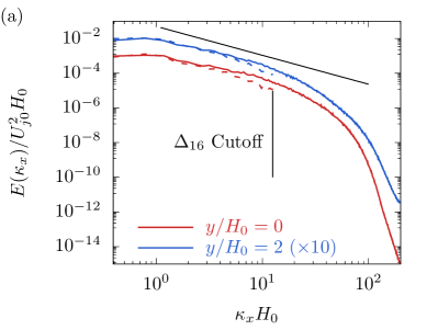
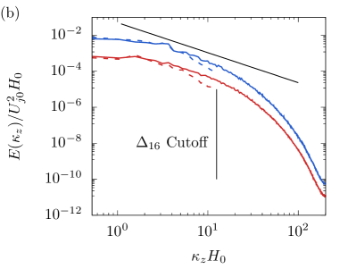
Figure 1: One-dimensional energy spectra from direct numerical simulation of a temporally evolving jet (case A; see table 1) at the centerline ($y/H_{0}=0$) and in the shear layer ($y/H_{0}=2$, shown offset by a factor of 10), at time $t=62.5t_{j0}$: (a) streamwise and (b) spanwise spectra. Dashed lines are the filtered direct numerical simulation data, with vertical lines indicating the $\Delta_{16}$ filter-cutoff wavenumber. Reference $\sim\kappa^{-5/3}$ lines are shown.

For the large-eddy simulations, (2.1) is replaced with either

$$\frac{\partial\overline{u}_{i}}{\partial t}+\overline{u}_{j}\frac{\partial\overline{u}_{i}}{\partial x_{j}}=-\frac{1}{\rho}\frac{\partial\overline{p}}{\partial x_{i}}+\nu\frac{\partial^{2}\overline{u}_{i}}{\partial x_{j}^{2}}-\frac{\partial\tau^{r}_{ij}}{\partial x_{j}},$$ (2.4)

for comparison with established $\tau_{ij}^{r}$ closure approaches, or (1.1), with the fitted neural network closure $h_{ij}$. For the anisotropic residual stress $\tau_{ij}^{r}=\tau_{ij}^{\text{{sgs}}}-\tau_{kk}^{\text{{sgs}}}\delta_{ij}/3$, we consider the Smagorinsky model[17, 18] with constant coefficient $C_{s}=0.18$, the dynamic Smagorinsky model[4, 5], and the model of Clark et al.[19]. Differently from a previous demonstration[11], where $\mathbf{h}$ modeled $\nabla\cdot\vec{\tau}\,^{r}$, here $h_{ij}$ models $\tau^{r}_{ij}$ directly for smoother optimization and greater modeling flexibility (§5.5). Moreover, it enables us to compare the functional form of $h_{ij}$ to traditional models (section 6).

The filter underlying the large-eddy simulation formulation is

$$\overline{\phi}(\mathbf{x},t)=\int_{\Omega}G(\mathbf{y},\mathbf{x})\phi(\mathbf{x}-\mathbf{y},t)\,d\mathbf{y},$$ (2.5)

though this is only explicitly used for comparison with direct numerical simulations and for generating large-eddy simulation initial conditions. For this, $G(\mathbf{y},\mathbf{x})$ has unit support in a ${\overline{\Delta}}$-cube centered on $\mathbf{x}$ [19].

2.2 Numerical discretization

Second-order centered differences are used on a staggered mesh [20], except for convective terms in the scalar equation (2.3), which were discretized using a third-order weighted essentially non-oscillatory (WENO) scheme [21]. Time integration is by a fractional-step method [22] and a linearized trapezoid method in an alternating-direction implicit (ADI) framework for the diffusive terms, as implemented by Desjardins et al.[23] Mesh densities for the direct numerical simulation cases listed in table 1 were selected so that the Kolmogorov scale $\eta=(\nu^{3}/\varepsilon)^{1/4}$, based on the calculated viscous dissipation rate $\varepsilon$, is resolved with uniform mesh spacing $\Delta x_{\text{{dns}}}$ such that $\Delta x_{\text{{dns}}}/\eta<1.8$ in the turbulence regions, which matches successful resolutions of turbulent jets at similar Reynolds number[24, 25, 26, 27, 28]. Spectra in figure 1 confirm that several decades of turbulence energy decay are resolved. The time step $\Delta t_{\text{{dns}}}$ was fixed, with initial CFL number about 0.37 that decreased to about 0.18 by the end of the simulation. A posteriori large-eddy simulations used the same numerical methods together with sub-grid-scale models or the deep learning model discussed subsequently in section 4. Analogous filtered spectra in figure 1 with $\Delta_{16}$ show a relatively high energy at the cutoff wavenumber. This substantially increases the modeling challenge, as is shown in section 3.3.

The adjoint-based neural network model training, which is described in section 4.2, uses the same numerical methods for the forward solution with the exception of time integration, which is by the fourth-order Runge–Kutta method for simplicity; thus the temporal adjoint solution is approximate. Since the overall order-of-accuracy is limited by the pressure-projection step, it is comparable to that of the forward solution. We further note that the adjoint solution is computed over only short time horizons (§4.2), for which the slightly different energy-conservation properties of the forward and adjoint time integrators do not become appreciable. An exact (in space only) discrete adjoint was solved.

3 Configurations

Free-shear-flow turbulence from multiple temporally developing planar jets, some with multiple streams, will be used for training and testing. These are introduced in the following subsections.

3.1 Turbulent plane jets

The baseline turbulent plane jet has a rounded top-hat initial streamwise mean velocity,

$$\hat{u}(y)=\frac{U_{j0}}{2}\left[\tanh\frac{y/H_{0}+1/2}{\delta_{L}}-\tanh\frac{y/H_{0}-1/2}{\delta_{L}}\right],$$ (3.1)

of width $\approx H_{0}$ bounded by shear layers of thickness $\approx\delta_{L}=0.1H_{0}$. The Reynolds number is $Re_{0}=U_{j0}H_{0}/\nu=6\,000$.

To seed transition to turbulence, spatially periodic fluctuations in the $x$–$z$ plane are added to the streamwise and cross-stream velocities:

$$\hat{\hat{u}}(y,z) =a\,\hat{u}(y)\cos\!\left[\frac{16\pi z}{L}\right]+\hat{u}(y)$$ (3.2)

$$\hat{\hat{w}}(x,y) =a\,\hat{u}(y)\cos\!\left[\frac{16\pi x}{W}\right],$$ (3.3)

where $a=0.1$, and $L$ and $W$ are the domain sizes in the periodic $x$- and $z$-directions, respectively (see table 1). Three-dimensional random perturbations are superimposed on top of these at each mesh point:

$$u(x,y,z) =\left[1+a(r_{x}(x,y,z)-0.5)\right]\hat{\hat{u}}(y,z)$$ (3.4)

$$w(x,y,z) =\left[1+a(r_{z}(x,y,z)-0.5)\right]\hat{\hat{w}}(x,y),$$ (3.5)

where $r_{x}$ and $r_{z}\in[0,1]$ are uniformly distributed. The initial cross-stream velocity is $v(x,y,z)=0$. This single-jet baseline case is case A in table 1.

Additional dual-jet cases, which are anticipated to involve entrainment and merging processes not seen in the single jet,[29] are used for out-of-sample tests. These additional processes occur over significantly longer duration than the development of approximate self-similarity in the single jet. Three specific dual-jet cases are considered: symmetric parallel jets (case B), asymmetric parallel jets (case C), and asymmetric anti-parallel jets (case D). These have initial streamwise mean velocity profile

$$\begin{split}\hat{u}(y)&=\frac{U_{j0}}{2}\left[\tanh\frac{(y+H_{s,0})/H_{0}+1/2}{\delta_{L}}-\tanh\frac{(y+H_{s,0})/H_{0}-1/2}{\delta_{L}}\right]\\ &+\frac{U_{j1}}{2}\left[\tanh\frac{(y-H_{s,1})/H_{1}+1/2}{\delta_{L,1}}-\tanh\frac{(y-H_{s,1})/H_{1}-1/2}{\delta_{L,1}}\right],\end{split}$$ (3.6)

where $H_{s}=\min(H_{0},H_{1})$, $H_{s,0}=(H_{s}+H_{0})/2$, $H_{s,1}=(H_{s}+H_{1})/2$, and $\delta_{L,1}=(H_{1}/H_{0})\delta_{L}$. The primary and secondary jets are set to have the same Reynolds number ($Re_{0}=Re_{1}$) based on their speed and width. Perturbations are superimposed following the same long-wavelength and random perturbations as for the single jet. Specific $H_{1}/H_{0}$ and $U_{j1}/U_{j0}$ ratios are listed in table 1.

Case	Configuration	$Re_{0}=U_{j0}H_{0}/\nu$	$H_{1}/H_{0}$	$U_{j1}/U_{j0}$	$(L,H,W)/H_{0}$	Uniform mesh
A	Single jet	6 000	–	–	$16,20,12$	$1024\times 1280\times 768$
B	Dual jets		1.0	1.0
C	Dual asym.		2.0	$+0.5$
D	Dual anti-para.		2.0	$-0.5$

Table 1: Conditions for the initial mean velocity profiles (3.1) for case A and (3.6) for cases B–D.

3.2 Jet evolution

Reynolds averages are over the periodic streamwise ($x$) and transverse ($z$) directions and are functions of the cross-stream ($y$) coordinate and time ($t$):

$$\langle{\phi}\rangle(y,t)=\frac{1}{L_{x}L_{z}}\int_{0}^{L_{x}}\int_{-L_{z}/2}^{L_{z}/2}\phi(x,y,z,t)\;dzdx,$$ (3.7)

with discrete analog

$$\langle{\phi}\rangle(y_{j},t^{n})=\frac{1}{N_{x}N_{z}}\sum_{i=1}^{N_{x}}\sum_{k=1}^{N_{z}}\phi(x_{i},y_{j},z_{k},t^{n}),$$ (3.8)

where $N_{x}$ and $N_{z}$ are the number of mesh points in the $x$- and $z$-directions. Subsequently presented large-eddy simulation results were also ensemble averaged in time using at least two realizations initialized with different random perturbations sampled from the same distributions.

The evolving centerline velocity $U_{cl}(t)\equiv\langle{u}\rangle(0,t)$ and half-width $y_{1/2}(t)$, defined by $\langle{u}\rangle(y_{1/2},t)=U_{cl}(t)/2$, are shown in figure 2 for the single jet (case A). There is an adjustment from the initial non-self-similar plug-like flow to an approximately linear spreading with $\sim t^{-1/2}$ centerline velocity decay for $t\gtrsim 15t_{j0}$, $t_{j0}=H_{0}/U_{j0}$, consistent with an onset of similarity. Spectra at $t=62.5t_{j0}$, such as are used subsequently for model evaluation, are shown in figure 1. The vorticity magnitude at $t=62.5t_{j0}$, as visualized in figure 3 (a), shows a range of large- and small-scale turbulence.

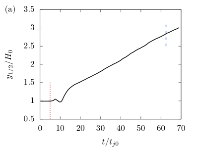
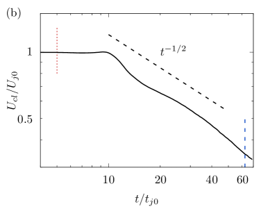
Figure 2: (a) Half-width and (b) centerline velocity of the case A jet direct numerical simulation. Subsequently discussed large-eddy simulations are initialized at $t=5t_{j0}$, indicated by dotted lines. Comparisons for this case are carried out at $t=62.5t_{j0}$, indicated by dashed lines.

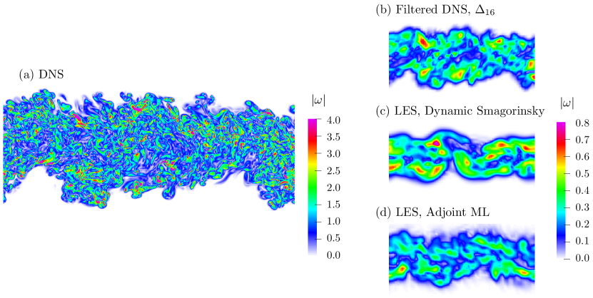
Figure 3: Vorticity magnitude at $z=0$ for $t=62.5t_{j0}$: (a) direct numerical simulation case A ($1024\times 1280\times 768$ mesh points); (b) the same field as (a) filtered using $\overline{\Delta}/\Delta_{\text{{dns}}}=16$ for an effective mesh of $64\times 80\times 48$ points; (c) large-eddy simulation using the dynamic Smagorinsky sub-grid-scale model, initialized at $t=5t_{j0}$ (see section 3.2), on $64\times 80\times 48$ mesh points; and (d) the analogous $64\times 80\times 48$ simulation on using the adjoint-trained deep learning model (section 4).

The large-eddy simulations are initialized by filtering the direct numerical simulation fields at $t=5t_{j0}$. As seen in figure 2, this is prior to the period of approximate self-similarity, which presumably increases the difficulty of matching statistics at later times. This initialization is also more representative of realistic LES, for which fully developed filtered-DNS initial conditions are typically unavailable. Primary comparisons for the single-jet case are made at $t=62.5t_{j0}$, which is approximately four times the time for first achieving approximate self-similarity based on the mean velocity. At this time, the jet has grown to approximately 2.75 times its original width. As an example, the vorticity magnitude of filtered DNS data is compared to large-eddy simulations using the dynamic Smagorinsky and adjoint-trained machine learning model in figures 3 (b–d). On this coarse grid, the learned model, described in section 4, produces turbulence that qualitatively better matches the filtered direct numerical simulation. Quantitative comparisons of these and other model predictions are presented in section 5.

Mean velocities for all cases are shown in figure 4. As expected, the single-jet profiles exhibit approximately self-similar evolution for $t\gtrsim 15t_{j0}$. However, the dual-jet cases do not, so a successful model will need to reproduce a presumably more challenging non-self-similar evolution. Subsequent quantitative comparisons for the dual-jet cases are at $t=50t_{j0}$ (case B) and $t=42.5t_{j0}$ (cases C and D).

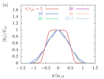
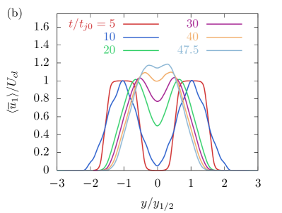
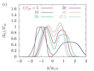
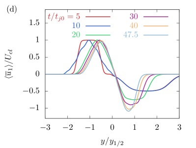
Figure 4: Mean streamwise velocity for (a) single jet (case A), (b) symmetric parallel jets (case B), (c) asymmetric parallel jets (case C), and (d) asymmetric anti-parallel jets (case D), all normalized by case A similarity variables. Profiles are shown starting at $t=5t_{j0}$.

3.3 Baseline sub-grid-scale models

The deep learning sub-grid-scale model is analyzed and compared primarily against a standard dynamic Smagorinsky model [4, 5]. Baseline performance of the dynamic Smagorinsky model is established by comparing with filtered direct numerical simulations. Since there is not explicit filtering during the large-eddy simulation, the nominal filter width and mesh resolution are equivalent: $\overline{\Delta}\equiv\Delta_{N}=N\Delta_{\text{{dns}}}$ [18].

Figure 5 shows mean streamwise velocity predictions of the single-jet case (A) for $\Delta_{N=16,8,4,2}$. The $\Delta_{16}$ case overpredicts the centerline velocity and underpredicts the jet spreading, though, as expected, agreement improves with finer meshes $\Delta_{8,4,2}$. This increases the separation between the dynamic-model test-filter scale and the large turbulence scales, thereby improving the realism of the isotropy assumption. The DNS mean filtered velocity is also shown in figure 5; this deviates only slightly from the unfiltered mean velocity.

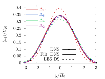
Figure 5: Direct numerical simulation, filtered DNS, and dynamic Smagorinsky (DS)[4] large-eddy simulation mean streamwise velocity $\overline{u}$ for the single jet (case A) at $t=62.5t_{j0}$ for filter sizes indicated: $\Delta_{16,8,4,2}$.

Budgets of turbulence kinetic energy provide a measure of the role of the models’ resolved-to-subgrid scale energy transfer versus viscous dissipation. Upon filtering, energy may be decomposed into resolved $E_{f}$ and residual (sub-grid-scale) $k_{r}$ components as

$$\overline{E}\equiv\frac{1}{2}\overline{u_{i}u_{i}}=\underbrace{\frac{1}{2}\overline{u}_{i}\overline{u}_{i}}_{E_{f}}+\underbrace{\frac{1}{2}\left(\overline{u_{i}u_{i}}-\overline{u}_{i}\overline{u}_{i}\right)}_{k_{r}}.$$ (3.9)

A gage of model importance can be inferred from the relative amounts viscous dissipation of $E_{f}$ by the resolved (filtered) velocity field

$$\varepsilon_{f}\equiv 2\nu\overline{S}_{ij}\overline{S}_{ij}$$ (3.10)

and the production rate of residual kinetic energy

$$P_{r}\equiv-\tau_{ij}^{r}\overline{S}_{ij}.$$ (3.11)

For both of these, $\overline{S}_{ij}$ is the filtered strain-rate. Both $\varepsilon_{f}$ and $P_{r}$ represent sink terms when positive.

Figure 6 compares the large-eddy simulation and filtered direct numerical simulation $\varepsilon_{f}$ and $P_{r}$ for the baseline jet. Ideally, $\varepsilon_{f}$ and $P_{r}$ should match the filtered direct numerical simulation values for the same filter size. As filter size increases, $\varepsilon_{f}$ is expected to decrease and $P_{r}$ to increase, and both do exhibit these trends. However, the dynamic Smagorinsky model increasingly overpredicts both $\varepsilon_{f}$ and $P_{r}$ with increasing filter size. This means that there is excessive removal of kinetic energy from the resolved scales. For $\Delta_{4}$, $P_{r}$ is a small fraction of $\varepsilon_{f}$, so the model for $\tau_{ij}^{r}$ plays only a minor role. The $\Delta_{4}$ filtered $\varepsilon_{f}^{\text{{dns}}}$ is about half the unfiltered dissipation $\varepsilon^{\text{{dns}}}$ (figure 6 a), so it dominates the evolution of the resolved kinetic energy. However, the balance is different for $\Delta_{16}$. Here, the sub-grid-scale production dominates the resolved dissipation, making the model essential. Such a challenge affords opportunities for improvement, so we focus on $\Delta_{16}$ for subsequent deep-learning modeling.

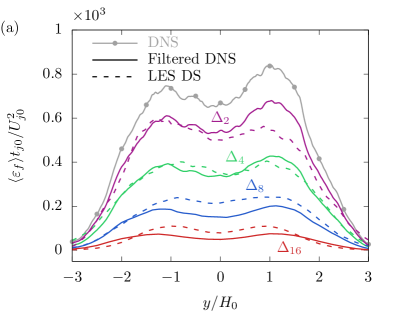
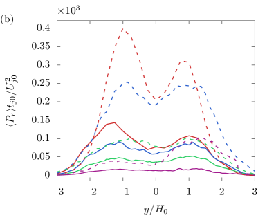
Figure 6: Evaluation of the dynamic Smagorinsky (DS) model for the baseline single jet (case A): (a) resolved viscous dissipation $\varepsilon_{f}$ (3.10) and (b) residual kinetic energy production rate $P_{r}$ (3.11) at $t=62.5t_{j0}$ for filter sizes indicated.

4 Neural-network Model and Training

The deep learning model architecture, hyperparameters, and training algorithm are described in this section. Section 4.1 presents the neural network model. Section 4.2 discusses the training algorithm.

4.1 Model architecture

We use a deep neural network $\mathbf{G}(\vec{\phi}\,(\mathbf{x},t);\vec{\theta}\,)$, where $\vec{\phi}\,$ represents space- and time-dependent input data from the running simulation, with the following architecture:

$$\begin{split}H^{1}&=\sigma(W^{1}\vec{\phi}\,+b^{1})\\ H^{2}&=\sigma(W^{2}H^{1}+b^{2})\\ H^{3}&=G^{1}\odot H^{2}\qquad\qquad\text{with}\quad G^{1}=\sigma(W^{5}z+b^{5})\\ H^{4}&=\sigma(W^{3}H^{3}+b^{3})\\ H^{5}&=G^{2}\odot H^{4}\qquad\qquad\text{with}\quad G^{2}=\sigma(W^{6}z+b^{6})\\ \mathbf{G}(\vec{\phi}\,;\vec{\theta}\,)&=W^{4}H^{5}+b^{4}\end{split}$$ (4.1)

where $\sigma$ is a $\tanh()$ element-wise nonlinearity, $\odot$ denotes element-wise multiplication, and the parameters are $\theta=\{W^{1},W^{2},W^{3},W^{4},W^{5},W^{6},b^{1},b^{2},b^{3},b^{4},b^{5},b^{6}\}$. The gated units $G^{1}$ and $G^{2}$ are chosen for their general capability to represent stiff, nonlinear behavior. Each layer includes $N_{\textsc{H}}=100$ hidden units, all initialized using a standard Xavier initialization [30]. Inputs to the neural network are normalized by the same set of constants for all cases.

In (1.1), $\mathbf{h}(\mathbf{x},t;\vec{\theta}\,)=\Psi(y)\mathbf{G}(\vec{\phi}\,(\mathbf{x},t));\vec{\theta}\,)$, where in the implementation $\Psi$ simply sets the neural network to zero at the $y=\pm H/2$ boundary mesh points.

We note that the discrete stress tensor $\mathbf{h}^{i,j,k}$ is not constrained to be exactly symmetric on the staggered mesh at finite resolution. Similarly, the symmetric sub-grid-scale stress components (e.g., $\tau^{r}_{12}$ versus $\tau^{r}_{21}$) appear in different equations ($x$- versus $y$-momentum), which are not exactly constrained by the same symmetries as the (unfiltered) Navier–Stokes equations.[2] Thus, further model flexibility in the finite-resolution limit may be achieved by relaxing the symmetry requirement. The same argument applies for corresponding tensor invariants; they will not hold for finite resolution, so are not imposed on the network. To be clear, as for any well-posed sub-grid-scale model, symmetry and invariance properties will be achieved with increasing resolution. Symmetry is revisited in section 5.5 and invariants in section 7.

The output $h^{i,j,k}_{ll}$ is at the cell center $\mathbf{x}=(i\Delta+\frac{\Delta}{2},j\Delta+\frac{\Delta}{2},k\Delta+\frac{\Delta}{2})$. For $l\neq m$, the output $h^{i,j,k}_{lm}$ is at the cell corners

$$\mathbf{x}=\begin{cases}(i\Delta,j\Delta,k\Delta+\frac{\Delta}{2}),&\textrm{if}\phantom{...}(l,m)=(1,2)\\ (i\Delta,j\Delta+\frac{\Delta}{2},k\Delta),&\textrm{if}\phantom{...}(l,m)=(1,3)\\ (i\Delta+\frac{\Delta}{2},j\Delta,k\Delta),&\textrm{if}\phantom{...}(l,m)=(2,3).\end{cases}$$ (4.2)

The derivatives $\frac{\partial h_{ij}}{\partial x_{j}}$ are then calculated at the cell faces using central differences with mesh-size $\Delta$, for example

$$\frac{\partial h_{11}}{\partial x}(i\Delta,j\Delta+\tfrac{\Delta}{2},k\Delta+\tfrac{\Delta}{2}) =\frac{h_{11}^{i,j,k}-h_{11}^{i-1,j,k}}{\Delta},$$

$$\frac{\partial h_{12}}{\partial y}(i\Delta,j\Delta+\tfrac{\Delta}{2},k\Delta+\tfrac{\Delta}{2}) =\frac{h_{12}^{i,j+1,k}-h_{12}^{i,j,k}}{\Delta},$$

$$\frac{\partial h_{13}}{\partial y}(i\Delta,j\Delta+\tfrac{\Delta}{2},k\Delta+\tfrac{\Delta}{2}) =\frac{h_{13}^{i,j,k+1}-h_{13}^{i,j,k}}{\Delta}.$$ (4.3)

Models were implemented and tested using two different sets of input variables. We first tested using $\vec{\phi}\,=(\overline{\mathbf{u}},\partial_{x_{l}}\overline{\mathbf{u}},\partial_{x_{l}x_{l}}\overline{\mathbf{u}})$ as an input, although this closure model is not Galilean invariant. For the simpler case of isotropic turbulence, for which this approach was first tested,[11] the model appeared to learn Galilean invariance. However, for the jets here, not surprisingly, it was found to be unstable in a posteriori simulations, at least for the amount of training evaluated. Therefore, a Galilean invariant form with $\vec{\phi}\,=(\partial_{x_{l}}\overline{\mathbf{u}},\partial_{x_{l}x_{l}}\overline{\mathbf{u}})$ was used here.

The input $\vec{\phi}\,$ to (4.1) for a large-eddy simulation grid cell $(i,j,k)$ includes the variables $\vec{\phi}\,^{i,j,k}$ for $(i,j,k)$ as well as the 6 adjacent cells. Velocity-gradient inputs are calculated using the same stencils as the convective and viscous operators. Thus, on-diagonal derivatives $\overline{u}_{l,l}$ are evaluated at cell centers, and off-diagonal derivatives $\overline{u}_{l,m},\ m\neq l$ are evaluated at cell faces. As an example,

$$\overline{u}_{1,x}(i\Delta+\tfrac{\Delta}{2},j\Delta+\tfrac{\Delta}{2},k\Delta+\tfrac{\Delta}{2}) =\frac{\overline{u}_{1}(i\Delta+\Delta,j\Delta+\frac{\Delta}{2},k\Delta+\frac{\Delta}{2})-\overline{u}_{1}(i\Delta,j\Delta+\frac{\Delta}{2},k\Delta+\frac{\Delta}{2})}{\Delta},$$

$$\overline{u}_{1,y}(i\Delta,j\Delta,k\Delta+\tfrac{\Delta}{2}) =\frac{\overline{u}_{1}(i\Delta,j\Delta+\frac{\Delta}{2},k\Delta+\frac{\Delta}{2})-\overline{u}_{1}(i\Delta,j\Delta-\frac{\Delta}{2},k\Delta+\frac{\Delta}{2})}{\Delta},$$

$$\overline{u}_{1,z}(i\Delta,j\Delta+\tfrac{\Delta}{2},k\Delta) =\frac{\overline{u}_{1}(i\Delta,j\Delta+\tfrac{\Delta}{2},k\Delta+\frac{\Delta}{2})-\overline{u}_{1}(i\Delta,j\Delta+\tfrac{\Delta}{2},k\Delta-\tfrac{\Delta}{2})}{\Delta}.$$ (4.4)

4.2 Training algorithm

A stochastic gradient descent-type scheme is employed, in which the adjoint partial differential equation is solved on random time sub-intervals $m=1,\ldots,M$ during each optimization iteration, each of which can be evaluated in parallel. The training algorithm is summarized below. We first consider the case in which we seek to minimize (1.6) as discussed in section 1 with $F(\overline{\mathbf{u}})=\overline{\mathbf{u}}(\mathbf{x},t)$. The extension to training on mean statistics is described in section 4.3.

• Initialize the parameters $\vec{\theta}\,^{0}$ with samples from the Xavier distribution [30].

• For training iteration $k=1,2,\ldots,K$:

  • Each sub-iteration $m=1,\ldots,M$ selects a random time $t^{m}$; the corresponding filtered direct numerical simulation data for $[t^{m},t^{m}+T_{s}]$ is taken as the training target: $F(\overline{\mathbf{u}}_{e})=\overline{\mathbf{u}}^{\text{{dns}}}$.

  • Equations (1.1) and (1.2) are solved over $[t^{m},t^{m}+T_{s}]$ with the filtered direct numerical simulation data at $t^{m}$ projected onto a divergence-free manifold as the initial condition.[11]

  • For each $m$, the adjoint is solved on $[t^{m}+T_{s},t^{m}]$ with objective function, rewritten from (1.6),

    $$L^{m}(\theta)=\int_{\Omega}\left\lVert\overline{u}^{\text{{dns}}}(t^{m}+T_{s},x)-\overline{u}(t^{m}+T_{s},x)\right\rVert\,d\mathbf{x}.$$ (4.5)

  • The adjoint solution provides the gradient $\nabla_{\vec{\theta}\,}L^{m}(\theta)$ for $m=1,\ldots,M$.

  • These $M$ gradients are averaged as $G=\displaystyle\frac{1}{M}\sum_{m=1}^{M}\nabla_{\theta}L^{L}(\theta)$.

  • The parameter $\vec{\theta}\,$ for the deep learning large-eddy simulation model is updated using the RMSprop algorithm[31] with the gradient $G$:

    $$\vec{r}^{k+1} =\rho\vec{r}^{k}+(1-\rho)G\odot G,$$

    $$\vec{\theta}\,^{k+1} =\vec{\theta}\,^{k}-\frac{\alpha^{k}}{\sqrt{\vec{r}^{k+1}}+\epsilon}\odot G,$$ (4.6)

    where $\alpha^{k}$ is the learning rate, and we take $\rho=0.99$ and $\epsilon=10^{-8}$. The $\sqrt{\vec{r}^{\ell+1}}$ operation is element-wise. The learning rate $\alpha^{k}$ is decreased by a factor of $\frac{1}{2}$ every $K$ iterations.

Taking $K=250$ and $M=12$ was found to be effective, though of course the optimal choice of such hyperparameters will generally depend upon the application and the model architecture. The time segments used had $T_{s}=5\Delta t_{\text{{les}}}$, with the large-eddy simulation time step $\Delta t_{\text{{les}}}=10\Delta t_{\text{{dns}}}$.

4.3 Training on the Reynolds-averaged statistics

As discussed in section 1, direct numerical simulation data, or correspondingly resolved experimental measurements, are not available in all cases. Therefore, as a relevant example of limited availability of data, we train a model only on the mean velocity and resolved Reynolds stresses: $F(\overline{\mathbf{u}})=(\langle{\overline{\mathbf{u}}}\rangle;\langle{{\overline{\mathbf{u}}^{\prime}\overline{\mathbf{u}}^{\prime}}}\rangle)(y,t)$. We obtain target data $F(\overline{\mathbf{u}}_{e})=(\langle{\overline{\mathbf{u}}^{\text{{dns}}}}\rangle;\langle{(\overline{\mathbf{u}}^{\prime}\overline{\mathbf{u}}^{\prime})^{\text{{dns}}}}\rangle)$ from the filtered case A, though in general measured data may be substituted without modification. In this case, the objective function becomes

$$L(\theta)=\frac{1}{L_{y}}\frac{1}{(T_{2}-T_{1})}\int_{T_{1}}^{T_{2}}\int_{0}^{L_{y}}\sum_{i=1}^{3}\frac{c_{1}}{U_{j0}^{2}}\bigg{(}\langle{\overline{u}_{i}^{{\text{{dns}}}}-\overline{u}_{i}}\rangle^{2}+\frac{c_{1}}{U_{j0}^{2}}\sum_{j=i}^{3}\langle{\overline{u}_{i}^{{\text{{dns}}}}\overline{u}_{j}^{{\text{{dns}}}}-\overline{u}_{i}\overline{u}_{j}}\rangle^{2}\bigg{)}\;dydt,$$ (4.7)

with $c_{1}=U_{j0}^{2}=467.4$ found to be effective for the current application. Training this objective function is computationally more challenging than with (4.5), since (4.7) requires solving the flow and its adjoint on the full $t\in[T_{1}=5,T_{2}=67.5]t_{j0}$ case A time horizon for each optimization iteration. Despite solving over a relatively long time length, the adjoint equation remains well-behaved.

5 Model Predictions

The objective functions, training data, and testing data for all cases are listed in table 2. We start in section 5.1 with an a priori $\tau_{ij}^{\text{{sgs}}}$ model, trained directly based on the sub-grid-scale stress mismatch (1.3). This simpler approach is demonstrated to be poor compared with the adjoint-based training in the following sections: in-sample results for the baseline case A jet (section 5.2) and out-of-sample analysis of cases B, C, and D (section 5.3). The performance for the averaged objective function (4.7) is assessed in section 5.4.

Objective Function ($F$)	Training	Testing	Section
$\tau_{ij}^{\text{{sgs}}}(\overline{\mathbf{u}})$	Jet (3.1)	Jet (3.1)	§5.1
(a priori ML)
$F(\overline{\mathbf{u}})=\overline{\mathbf{u}}(\mathbf{x},t)$	Jet (3.1)	Jet (3.1)	§5.2
(filtered velocity)		Dual jets (3.6)	§5.3
		Dual asymmetric (3.6)	§5.3
		Dual anti-parallel (3.6)	§5.3
$F(\overline{\mathbf{u}})=(\langle{\overline{\mathbf{u}}}\rangle;\langle{{\overline{\mathbf{u}}^{\prime}\overline{\mathbf{u}}^{\prime}}}\rangle)_{(y,t)}$	Jet (3.1)	Jet (3.1)	§5.4
($x$ and $z$ averaged)		Dual jets (3.6)
		Dual asymmetric (3.6)
		Dual anti-parallel (3.6)
$F(\overline{\mathbf{u}})=\overline{\mathbf{u}}(\mathbf{x},t)$	Jet (3.1)	Jet (3.1)	§5.5
(filtered velocity; $h_{ij}=h_{ji}$)		Dual jets (3.6)
		Dual asymmetric (3.6)
		Dual anti-parallel (3.6)

Table 2: Objective functions, training data, and testing data for primary cases studied.

5.1 A priori training

The model of section 4.1 is trained to minimize the a priori mismatch between the modeled and filtered direct numerical simulation $\tau_{ij}^{\text{{sgs}}}$. This is the simple, direct approach: training requires only 5.5 hours on 24 Nvidia K20X GPU nodes. The a priori $\tau_{ij}^{\text{{sgs}}}$ agreement in figure 7 (a) is good, as expected since deep neural networks are well-understood to fit data well. However, this fit is unconstrained by the how the model interacts with the governing equations, so it is unsurprising that the a posteriori performance in a large-eddy simulation is poor (figure 7 b), even for the mean velocity. Simply minimizing the mismatch is insufficient, even for this relatively simple free-shear flow. In figure 7 (b), the adjoint-trained neural network with $F(\overline{\mathbf{u}})=\overline{\mathbf{u}}$, which is discussed subsequently, performs far better for the same network model.

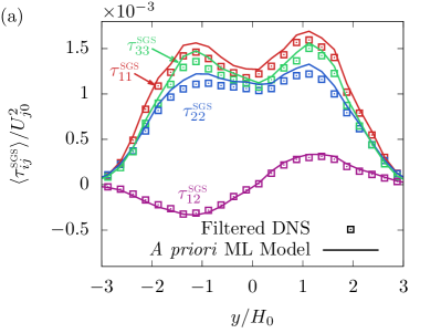
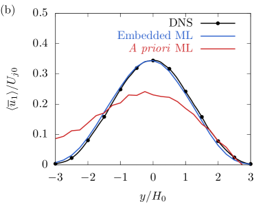
Figure 7: The a priori-trained deep learning model for case A for $\Delta_{16}$ at $t=62.5t_{j0}$: (a) residual stress agreement from filtered direct numerical simulations and the a priori-trained model, and (b) predicted mean streamwise velocity.

5.2 Single-jet case (in-sample)

In this case, the model is trained on filtered instantaneous velocity fields ($F(\overline{\mathbf{u}})=\overline{\mathbf{u}}(\mathbf{x},t)$) from case A and tested on the same configuration. In figure 8 (a), we see that for $\Delta_{16}$ the deep learning model nearly perfectly reproduces the mean velocity, doing better than the dynamic Smagorinsky (DS) model for the coarse $\Delta_{16}$ case and comparably to it for $\Delta_{8}$. In figure 8 (b), it also better tracks the evolution of $y_{1/2}$: for both $\Delta_{8}$ and $\Delta_{16}$, the dynamic Smagorinsky model underpredicts jet spreading at early times.

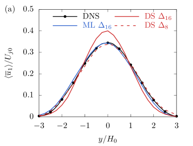
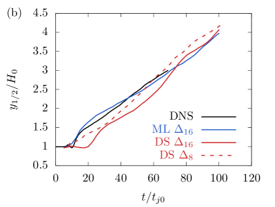
Figure 8: Single jet (case A) in-sample comparison for learning (ML) and dynamics Smagorinsky (DS) models: (a) mean streamwise velocity $\overline{u}_{1}$ at $t=62.5t_{j0}$ and (b) half-width $y_{1/2}$ evolution for the indicated filter sizes. The direct numerical simulation data are included for comparison.

Resolved Reynolds stress components $R_{ij}\equiv\langle{\left(\overline{u}_{i}-\langle{\overline{u}_{i}}\rangle\right)\left(\overline{u}_{j}-\langle{\overline{u}_{j}}\rangle\right)}\rangle$ are compared in figure 9. As expected, based on the mean-flow evolution, the trained model significantly outperforms dynamic Smagorinsky at this coarse resolution. The complete Reynolds stress from the direct numerical simulation, prior to filtering to match the large-eddy simulation model, is also shown to quantify the sub-grid-scale contribution to the turbulence stresses. One-dimensional energy spectra in figure 10 confirm that the deep learning model more accurately reproduces the spectral energy distribution than the dynamic Smagorinsky model, and this is particularly evident at high wavenumbers.

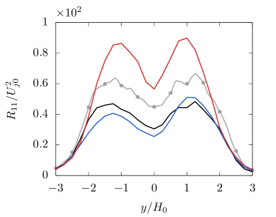
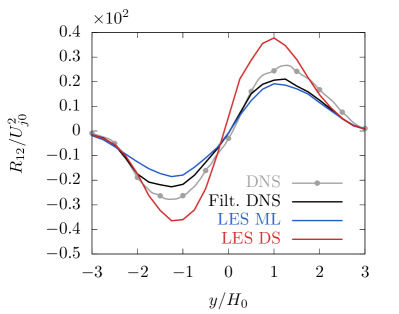
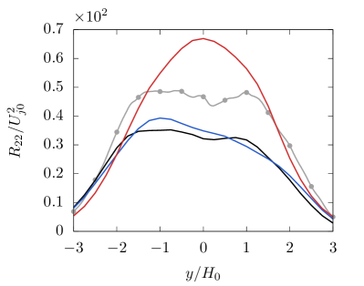
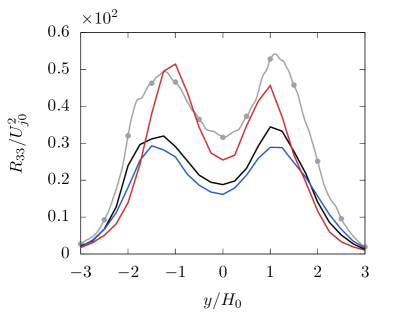
Figure 9: Resolved Reynolds stress components as labeled in the single-jet case A at $t=62.5t_{j0}$ for $\Delta_{16}$: the new learning model (ML), dynamic Smagorinsky (DS), and the filtered direct numerical simulation (DNS). The unfiltered Reynolds stress components are also shown for reference.

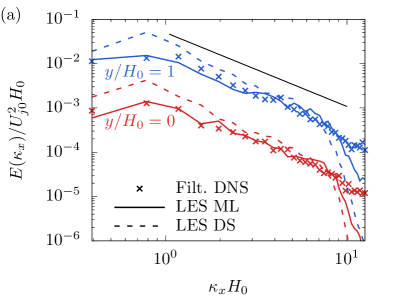
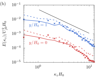
Figure 10: (a) Streamwise and (b) spanwise energy spectra for the single-jet case A with $\Delta_{16}$ at $t=62.5t_{j0}$: filtered (DNS), machine learning model (ML), and dynamic Smagorinsky (DS). The straight lines have $\kappa^{-5/3}$ slope. Spectra are shown at the centerline ($y/H_{0}=0$) and at $y/H_{0}=1$, which corresponds to the cross-stream location of maximum resolved kinetic energy is shown offset by a factor of 10.

5.3 Dual-jet cases (out-of-sample)

Out-of-sample mean-flow results are shown in figure 11 for all three dual-jet cases of table 1. The corresponding resolved viscous dissipation rates are shown in figure 12.

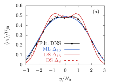
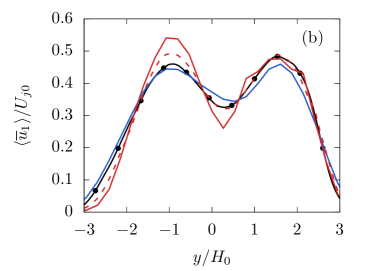
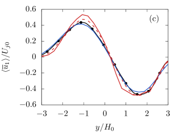
Figure 11: Out-of-sample mean streamwise velocity $\overline{u}_{1}$ for $\Delta_{16}$ and the deep learning (ML) and dynamic Smagorinsky (DS) models: (a) case B at $t=50t_{j0}$, (b) case C at $t=42.5t_{j0}$, and (c) case D at $t=42.5t_{j0}$. The $\Delta_{8}$ case is shown for reference.

For the symmetric parallel jets case B, the deep learning model on $\Delta_{16}$ has accuracy comparable to the dynamic Smagorinsky model on $\Delta_{8}$ and predicts the resolved viscous dissipation rate. It is thus predicts the merging process for which it was not trained. Conversely, for this resolution, the dynamic Smagorinsky model on the coarse $\Delta_{16}$ mesh substantially underpredicts the jet merging, showing two distinct peaks of mean velocity. Similarly to case A, this corresponds to over-prediction of $\varepsilon_{f}$ near the high-shear regions.

The overall performance for the asymmetric parallel jets (case C) is similarly good: the coarse-grid deep learning model more accurately reproduces the jet spreading than the dynamic Smagorinsky model for both $\Delta_{16}$ and $\Delta_{8}$ (figure 11 b). Of the three models, the deep learning model also most accurately reproduces the peak velocity of the lower jet ($y\approx-H_{0}$), though at the same time it less accurate for the peak velocity of the slower-speed upper jet ($y\approx 2H_{0}$). This might be because the lower jet more closely matches the training case A, whereas the upper jet is slower ($U_{1}=U_{0}/2$) and wider ($H_{1}=2H_{0}$), as seen in table 1 and figure 4. These trends are repeated in figure 12 (b) for the resolved dissipation rate.

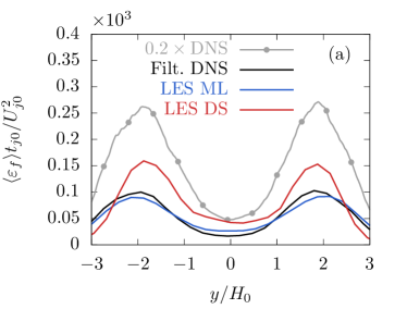
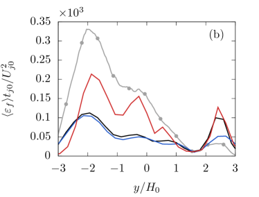
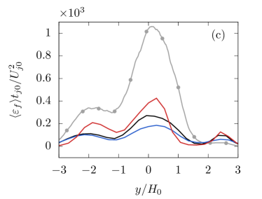
Figure 12: Out-of-sample resolved viscous dissipation $\varepsilon_{f}$ for the deep learning (ML) and dynamic Smagorinsky (DS) models for $\Delta_{16}$: (a) case B at $t=50t_{j0}$, (b) case C at $t=42.5t_{j0}$, and (c) case D at $t=42.5t_{j0}$. The unfiltered direct numerical simulation viscous dissipation rate $\times 0.2$ is shown for comparison.

The deep learning model similarly outperforms the dynamic Smagorinsky model in the asymmetric, anti-parallel jets (case D) (figures 11 c and 12 c), for both $\Delta_{16}$ and $\Delta_{8}$. Unlike previous cases, this configuration has much larger $\varepsilon_{f}$ in the high-shear, inter-jet region ($y\approx 0$) than in the jets themselves. The deep learning model performs especially well in this region.

One-dimensional energy spectra in figure 13 show that the deep learning model performs particularly well at high wavenumbers. This might follow from the ability of the deep learning model to compensate for discretization errors, as considered for isotropic turbulence[11]. As can be seen in figure 13, the deep learning model nearly eliminates unphysical near-cutoff-wavenumber dissipation.

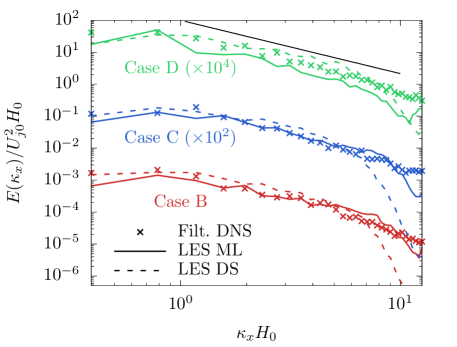
Figure 13: Out-of-sample one-dimensional streamwise energy spectra at the point of peak resolved turbulence kinetic energy for $\Delta_{16}$ at $t=50t_{j0}$ for case B, at $t=42.5t_{j0}$ for case C, and at $t=42.5t_{j0}$ for case D. The straight line has $\kappa^{-5/3}$ slope.

5.4 Training for mean statistics

It is, of course, expected that the reduced information content in this case will make training sub-grid-scale turbulence models more challenging. We take $F(\overline{\mathbf{u}})=(\langle{\overline{\mathbf{u}}}\rangle;\langle{{\overline{\mathbf{u}}^{\prime}\overline{\mathbf{u}}^{\prime}}}\rangle)_{(y,t)}$, leading to the loss function (4.7) developed in section 4.3 trained on the single-jet case A. This corresponds to the third set of tests in table 2. The same neural network architecture (section 4.1) and training algorithm (section 4.2) are used as for the previous demonstrations.

The results for the mean flow are shown in figure 14. In all cases, the model produces a reasonable prediction, unlike the a priori training on the mismatch of section 5.1. And, as expected, it performs well in-sample, which is expected since it was trained specifically to match its Reynolds stress data. For the out-of-sample symmetric dual-jet (case B), is also performs comparably to the model trained on the filtered data. However, with its less rich training set, it is not expected to extrapolate as well as the model trained with the richer three-dimensional filtered data. For the asymmetric out-of-sample jets (cases C and D), it only closely matches the data on the sides of the dual-jets that are similar to the case A training data ($y<0$; see table 1 and figure 4). On the other sides, the model overpredicts spreading, though not catastrophically, despite the huge reduction of training data size: the mean flow statistics have $N_{x}N_{z}$ times fewer degrees of freedom per (3.8) than the instantaneous velocity. It might be anticipated that expanded training data sets are likely necessary for this approach to be more accurate. Additional implications of the mean-statistics training are discussed in section 7.

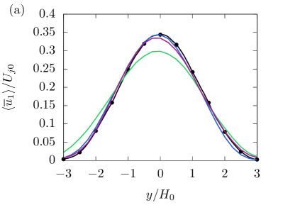
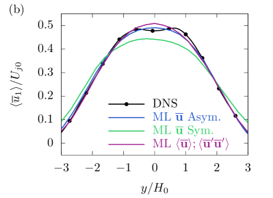
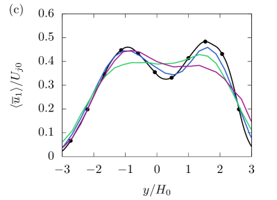
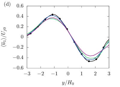
Figure 14: Mean-flow development for training with (4.7) mean statistics (see table 2) for $\Delta_{16}$: in-sample (a) case A at $t=62.5t_{j0}$ and out of sample (b) case B at $t=50t_{j0}$, (c) case C at $t=42.5t_{j0}$, and (d) case D at $t=42.5t_{j0}$. Results for the baseline instantaneous field training (ML $\overline{\mathbf{u}}$ Asym.) and its symmetrically constrained variant of section 5.5 (ML $\overline{\mathbf{u}}$ Sym.) are also shown.

5.5 A symmetric constraint

As introduced in section 4.1, the models discussed up to this point were not constrained to produce symmetric stress outputs, which is not a rigid constraint for typical discretizations of the governing equations. Corresponding results for a model that is trained to match the filtered velocity from case A ($F(\overline{\mathbf{u}})=\overline{\mathbf{u}}$), but now exactly constrained to produce symmetric stresses ($h_{ij}=h_{ji}$), are shown figure 14 for both in-sample and out-of-sample cases. Its performance is markedly worse than either previous model in most circumstances. This highlights performance gained by relaxing the symmetry constraint, which is not consistent with the discretized form of the governing equations.

6 The $\mathbf{h}$ Closure

With the trained model working effectively in testing cases, especially when the training is based on the filtered instantaneous data, it is natural to analyze its form. As for any deep-learning model, it is difficult to infer the mode of its operation, which in turn risks hindrance of its physical interpretation for flows.[10] However, we can make some assessment of it. Here, we develop simplified functional forms based on $\mathbf{h}$ from the trained neural network by calibrating candidate functional forms $\mathbf{g}$ that minimize

$$J(\vec{\phi}\,)=D\left(\mathbf{h}(\overline{\mathbf{u}};\vec{\theta}\,),\mathbf{g}(\overline{\mathbf{u}};\vec{\phi}\,)\right),$$ (6.1)

as determined by a linear least-squares fit. Each candidate closure $\mathbf{g}$ has a low-dimensional set of parameters $\vec{\phi}\,$ that are fitted to the $\mathbf{h}$ trained for $F(\overline{\mathbf{u}})=\overline{\mathbf{u}}$ based on evaluation at all mesh and time points in case A. Attempts to interpret the fitted models are then made, and several of these $\mathbf{h}$-fitted models are implemented for a posteriori tests.

We start with a Taylor series expansion in filter width including terms up to $O(\overline{\Delta}^{2})$, which thus has 39 parameters per $\tau^{r}_{ij}$ component (351 total):

$$g_{ij}(\overline{\mathbf{u}})=a_{ijk}\overline{u}_{k}+\overline{\Delta}b_{ijkl}\frac{\partial\overline{u}_{k}}{\partial x_{l}}+\overline{\Delta}^{2}c_{ijklm}\frac{\partial^{2}\overline{u}_{k}}{\partial x_{l}\partial x_{m}}.$$ (6.2)

This expansion for two sub-grid-scale stress components is shown in figure 15. We focus on components for which the deep learning model learns asymmetries (discussed in section 4), with $\tau^{r}_{12}$ and $\tau^{r}_{21}$ shown in figure 15 as an example, though we made analogous observations for all other components. The Taylor-series model (6.2) is able to reproduce the asymmetries learned by $\mathbf{h}$ and, roughly, its variances. Other model forms, such as those discussed subsequently based on the Smagorinsky and Clark models, are unable to do so. There seem to be two aspects to the relative success of (6.2): (1) assigning separate parameters to asymmetric velocity gradient tensors (and not using the symmetric strain-rate tensor $S_{ij}$) and (2) including all velocity derivatives in $g_{ij}$, not just those with the same $i,j$ indices. One would expect that asymmetries in decoupled closures (for example, those based on the Boussinesq hypothesis) could be learned simply by including the asymmetric velocity derivatives. However, the improvements of including non-index-matching velocity derivatives reinforces the idea that $\mathbf{h}$ can learn inter-PDE couplings, consistently with the overall discretization of the equations.

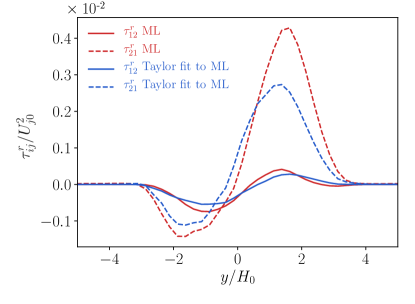
Figure 15: Taylor-series expansion $\mathbf{g}$ from (6.2) fitted to the deep learning (ML) model outputs $\mathbf{h}$ for the $\tau_{12}$ and $\tau_{21}$ non-symmetric model components.

We can also infer properties of $\mathbf{h}$ by fitting it with the functional forms of standard low-degree-of-freedom turbulence models. We first consider the constant-coefficient Smagorinsky model,[17, 18]

$$\tau^{r,\mathrm{Smag}}_{ij}=-2C_{s}^{2}\overline{\Delta}^{2}|\overline{S}|\left(\overline{S}_{ij}-\frac{1}{3}\overline{S}_{kk}\delta_{ij}\right),$$ (6.3)

where $|\overline{S}|=(2\overline{S}_{ij}\overline{S}_{ij})^{1/2}$ is the filtered strain-rate magnitude. The fitting parameter is $\vec{\phi}\,=[C_{s}^{2}]$. With all components of the model denoted $\vec{\tau}\,^{r,\mathrm{Smag}}=\mathbf{a}(\overline{\mathbf{u}})\vec{\phi}\,$, we can obtain $C_{s}$ by minimizing (6.1). For case A, this yields $C_{s}=0.163$ for $\mathbf{h}(\overline{\mathbf{u}};\vec{\theta}\,)$ and $C_{s}=0.118$ for $\vec{\tau}\,^{r}_{\text{{dns}}}$, both of which are comparable to common values. Simulation results for these candidate coefficients are shown in figure 16 (a). The coefficient learned from $\mathbf{h}$, $C_{s}=0.163$, most accurately reproduces the mean flow of the three. The learned coefficients ($C_{s}=0.163$ and $C_{s}=0.118$) also more correctly reproduce jet spreading (not shown), but not as accurately as the full neural-network model.

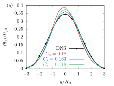
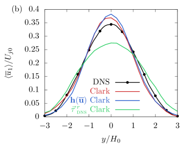
Figure 16: Performance on case A of baseline, $\mathbf{h}$-fitted, and $\overline{u}$-fitted models at $t=62.5t_{j0}$ and for $\Delta_{16}$: (a) the constant-coefficient Smagorinsky model ($C_{s}=0.163$: $\mathbf{h}$-fit; $C_{s}=0.118$: $\vec{\tau}\,^{r}_{\text{{dns}}}$-fit), and (b) the Clark model (see text).

We also consider the model of Clark et al.[19], which is obtained via a Taylor-series expansions of $\vec{\tau}\,^{r}$ in filter size $\overline{\Delta}$:

$$\tau^{r,\mathrm{Clark}}_{ij} =\tau^{r,\mathrm{Smag}}_{ij}+\tau^{r,\mathrm{grad}}_{ij}$$

$$=\tau^{r,\mathrm{Smag}}_{ij}+\frac{1}{12}\left(\overline{\Delta}^{2}\frac{\partial\overline{u}_{i}}{\partial x_{k}}\frac{\partial\overline{u}_{j}}{\partial x_{k}}-\frac{\overline{\Delta}^{2}}{3}\frac{\partial\overline{u}_{k}}{\partial x_{k}}\frac{\partial\overline{u}_{k}}{\partial x_{k}}\delta_{ij}\right).$$ (6.4)

The second term on its own is known as the gradient model, which, while accurate in a priori evaluations because it provides a good approximation for filter-scale perturbations in an ideally filtered DNS field, can cause numerical instabilities in a posteriori evaluation.[32]

To fit coefficients with $\vec{\phi}\,=[C_{s}^{2},C_{g}]^{T}$, we rewrite (6.4) as

$$\vec{\tau}\,^{r,\mathrm{Clark}}=C_{s}^{2}\,\mathbf{a}_{\mathrm{Smag}}(\overline{\mathbf{u}})+C_{g}\,\mathbf{a}_{\mathrm{grad}}(\overline{\mathbf{u}}).$$ (6.5)

With $\mathbf{a}(\overline{\mathbf{u}})=[\mathbf{a}_{\mathrm{Smag}},\mathbf{a}_{\mathrm{grad}}]$, the model is $\vec{\tau}\,^{r,\mathrm{Clark}}=\mathbf{a}(\overline{\mathbf{u}})\vec{\phi}\,$. Fitting to $\mathbf{h}(\overline{\mathbf{u}})$ yields $C_{s}=0.151$ and $C_{g}=0.422$, and fitting to $\vec{\tau}\,^{r}_{\text{{dns}}}$ yields $C_{s}=0.041$ and $C_{g}=1.288$. Of these, only the fit to $\mathbf{h}(\overline{\mathbf{u}})$ appears reasonable based on typical values. This is a surprise, since one might expect that the coefficients could be learned directly from the filtered data. However, the same assumption is the reason a priori evaluation often incorrectly predicts a model’s a posteriori performance. A posteriori results are shown in figure 16 (b). With $\mathbf{h}$-learned coefficients, results are comparable to the unity-coefficient model, and, indeed, the DNS-fitted coefficients are inaccurate.

These results suggest that high-degree-of-freedom models can be interpreted in the context of pre-specified functional forms. In particular, we observe that asymmetries in the modeled sub-grid-scale stress can be codified using asymmetric velocity gradient tensors, and that $\mathbf{h}$ might learn inter-PDE couplings between the different velocity components. However, low-degree-of-freedom attempts to interpret highly parameterized models will often be found wanting, and this can be seen in attempts to fit standard turbulence-model parameters to the neural network form. While these can produce better-performing fitted (or at least not seriously performance degrading) parameters, they do not match the a posteriori accuracy of the full model.

7 Predicted Turbulence Structure

The agreement of the deep learning model prediction with the usual statistical measures (mean, turbulence stresses, energy spectrum) suggests an improved representation of realistic turbulence at the resolved scales. Whether or not this agreement translates to an improved representation of the turbulence structure, which would be important for extrapolation beyond the training metrics, is quantified with barycentric maps. These track the eigenvalue invariants of the normalized resolved Reynolds stress anisotropy $a_{ij}=R_{ij}/R_{kk}-\delta_{ij}/3$,[33] and as such quantify resolved turbulence componentiality. Though an obvious downside for neural network models is the lack of proof about realizability and boundedness, barycentric maps offer an empirical assessment of this: the lines connecting the vertices of such maps are physical bounds, and remaining within them is not guaranteed. One could envision that a deep learning model might, despite a PDE constraint, sacrifice physical realism for a good fit to data; this is tested in this section. The degree to which a deep learning closure recovers the ideal turbulence structure supports its extrapolative capacity and its additional adherence to the physics beyond reproduction of the training data.

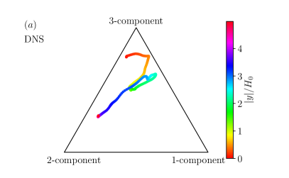
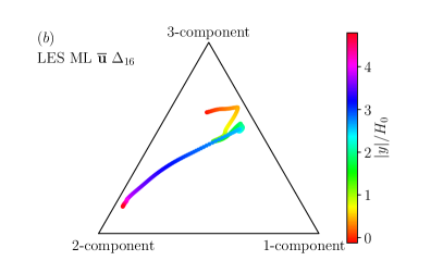
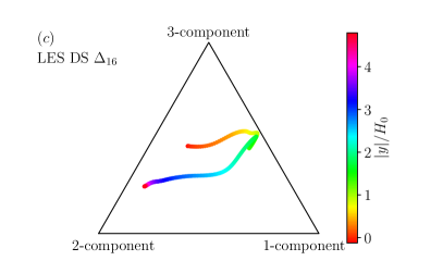
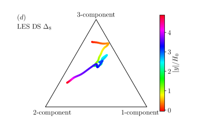
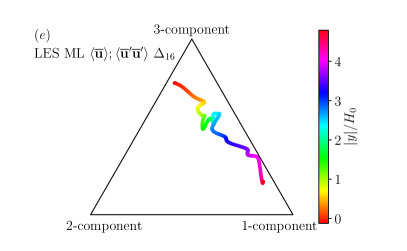
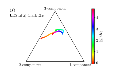
Figure 17: Barycentric maps of normalized resolved Reynolds stress invariants at various cross-stream locations $|y|/H_{0}$ for case A at $t=62.5t_{j0}$, with data averaged $\pm y$: (a) direct numerical simulation, (b) machine learning model with $\mathbf{h}(\overline{\mathbf{u}})$ (see table 2), (c–d) the dynamic Smagorinsky model fo $\Delta_{16,8}$, (e) training on averaged statistics $F(\overline{\mathbf{u}})=(\langle\mathbf{u}\rangle;\langle\overline{\mathbf{u}}^{\prime}\overline{\mathbf{u}}^{\prime}\rangle)$ (see table 2), and (f) the Clark model fitted to $\mathbf{h}(\overline{\mathbf{u}})$ (see section 6).

Barycentric maps for the case A resolved turbulence and $\Delta_{16}$ machine-learning model are shown in figures 17 (a) and (b). All trajectories remain within the physical bounds, and this is also the case for the dual-jet configurations (not shown). The trajectories within the maps show the variation of componentiality in $y$. Key features of the direct numerical simulation (figure 17 a) include a relative two-component condition in the outer shear layers ($|y|\approx 4H_{0}$), predominantly plane-strain (the line bridging three- and two-componentiality) within the shear layers, and three-component turbulence near the centerline ($|y|\lesssim H_{0}$). Also shown are invariant maps of a posteriori large-eddy simulation using the dynamic Smagorinsky model, the $F(\overline{\mathbf{u}})=(\langle\mathbf{u}\rangle;\langle\overline{\mathbf{u}}^{\prime}\overline{\mathbf{u}}^{\prime}\rangle)$ closure, and the $\mathbf{h}(\overline{\mathbf{u}})$-fitted Clark model. Both the $\Delta_{16}$ $\mathbf{h}(\overline{\mathbf{u}})$ states (figure 17 b) and $\Delta_{8}$ dynamic Smagorinsky states (figure 17 d) show the general features of the direct numerical simulation, consistent with the ability of these models to reproduce other turbulence statistics. However, the coarse $\Delta_{16}$ dynamic Smagorinsky model (figure 17 c) fails to achieve the same three-componentiality for $|y|\rightarrow 0$.

Trajectories obtained using $\mathbf{h}$ trained with only mean statistics ($F(\overline{\mathbf{u}})=(\langle\mathbf{u}\rangle;\langle\overline{\mathbf{u}}^{\prime}\overline{\mathbf{u}}^{\prime}\rangle)$) in figure 17 (e) only recover the turbulence structure for $|y|\lesssim H_{0}$. This case fails to recover the two-component limiting conditions in the outer shear layers ($|y|/H_{0}\approx 4$), instead trending toward one-component turbulence. More training data from richer flows might remedy this.[7]

Finally, invariant trajectories of the $\mathbf{h}(\overline{\mathbf{u}})$-fitted Clark model from section 6 are shown in figure 17 (f). Despite its apparently good mean-flow prediction (figure 16 b), the turbulence produced bears little resemblance the direct numerical simulation data. Thus, this model is not expected to be extrapolative, efforts for which will likely benefit from better faithful representation of the turbulence structure in addition to any particular statistics. For example, subfilter models for reacting flows will almost certainly benefit from the capability to encode these dynamics.[34, 35] As a step toward assessing, out-of-sample tests of the $\mathbf{h}$-fitted Clark model are presented along with the machine-learning model for scalar mixing in the following section.

8 Mixing of a Passive Scalar

In section 5.1, it was shown that the high-dimensional neural-network model could, not surprisingly, fit the filtered direct numerical simulation sub-grid-scale stresses through a direct mismatch loss function, though this fitted stress failed to provide a viable mode when subsequently used in a simulation. This exemplifies the risk of fitting without physical constraints, which guard against overfitting and unreliability for extrapolative prediction. Optimizing the model as embedded in the governing equation (sections 5.2 and 5.3) provided a model that reproduced turbulence statistics for a class of similar flows, demonstrating some capacity for reliable extrapolation. Here, we further evaluate the extrapolative capacity of the model by assessing passive scalar $\xi$ mixing predictions. Filtering (2.3) yields

$$\frac{\partial\overline{\xi}}{\partial t}+\overline{u}_{j}\frac{\partial\overline{\xi}}{\partial x_{j}}=D\frac{\partial^{2}\overline{\xi}}{\partial x_{j}^{2}}-\frac{\partial}{\partial x_{j}}\left(\overline{u_{j}\xi}-\overline{u}_{j}\overline{\xi}\right),$$ (8.1)

where $D=0$. Only numerical diffusion was active in both the direct numerical simulation and the large-eddy simulation, and then only for the scalar advection. The second term on the right-hand side of (8.1) is the divergence of the unclosed residual scalar flux $F_{j}^{\xi}=\overline{u_{j}\xi}-\overline{u}_{j}\overline{\xi}$. We model $F_{j}^{\xi}$ using the gradient-diffusion hypothesis, in which the eddy diffusivity is obtained using a scalar analog of the dynamic Smagorinsky model [4].

The predicted mean scalar profiles for the four jet cases, simulated with $\vec{\tau}\,^{r}$ obtained from either the deep learning model, the dynamic Smagorinsky model, or the $\mathbf{h}$-fitted Clark model, are evaluated in figure 18. The deep learning model outperforms the others in all four cases. This is particularly evident in the double-jet cases, for which the same $\Delta_{16}$ using dynamic Smagorinsky underpredicts jet spreading and merging (see figure 11). This result is comparably accurate to dynamic-Smagorinsky predictions for $\Delta_{8}$. Conversely, the $\mathbf{h}$-fitted Clark model, with coefficients obtained for case A, performs poorly for the out-of-sample dual-jet cases.

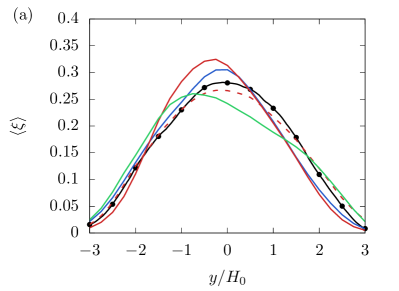
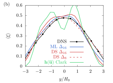
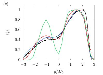
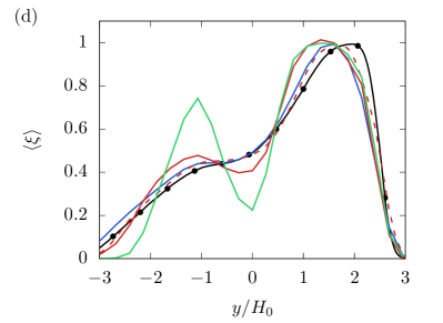
Figure 18: Mean passive scalar for the deep learning (ML), dynamic Smagorinsky (DS), and $\mathbf{h}$-fitted Clark model for $\vec{\tau}\,^{r}$ for $\Delta_{16}$ for (a) case A at $t=62.5t_{j0}$, (b) case B at $t=50t_{j0}$, (c) case C at $t=42.5t_{j0}$, and (d) case D at $t=42.5t_{j0}$. For comparison, $\Delta_{8}$ DS results are also shown.

The results in this section provide evidence of potentially improved predictive accuracy of coupled-PDE simulations using the deep learning model. However, we note that the more complicated case of two-way-coupled PDEs has yet to be investigated. Variable-density, non-reacting scalar mixing, with a simple equation of state, is an obvious next step in analyzing two-way couplings.

9 Mesh-dependence

We finally consider the effect of different grid resolutions on the learned closure $\mathbf{h}$. The a priori convergence of $\mathbf{h}$ outputs with grid refinement is first shown. Then, a posteriori performance of the model on finer grids, for which the model was not explicitly trained, is assessed.

9.1 Convergence with grid refinement

The preceding sections center around implicitly filtered large-eddy simulation, $\Delta_{\text{{les}}}/\Delta_{\text{{dns}}}=\overline{\Delta}/\Delta_{\text{{dns}}}$, where $\Delta_{\text{{dns}}}$ and $\Delta_{\text{{les}}}$ distinguish the fine direct numerical simulation mesh and large-eddy simulation meshes. For constant $\overline{\Delta}$, we now consider a priori convergence of sub-grid-scale closure approximations with refinement of $\Delta_{\text{{les}}}$. This enables estimation of discretization errors and the degree to which $\mathbf{h}$ deviates from the expected convergence of the differential approximation of the underlying numerical scheme.

For constant $\overline{\Delta}$, standard models for $\vec{\tau}\,^{r}$ converge as $O(\Delta_{\text{{les}}}^{p})$ for order-$p$ spatial discretizations. Here, $p=2$. The deep learning model is not constrained by this: as described in section 4.1, although its inputs are the velocity first and second derivatives at adjacent mesh points, it is nonlinear and so not constrained to show second-order convergence, at least for the resolutions we test. In theory, it can compensate for coarse-grid truncation error in a posteriori large-eddy simulation, for which numerical errors appear as additional, unclosed terms when compared to trusted target data[11].

Velocity gradients are computed from filtered direct numerical simulation data for $\overline{\Delta}=\Delta_{16}$. The finite-difference approximations are evaluated for $\Delta_{\text{{les}}}/\Delta_{\text{{dns}}}=16,8,4,2,1$ using the same staggered variable placement as the solver (see section 2.2).

To quantify the mesh convergence of the different closures, a relative difference[36] is computed as

$$\varepsilon_{\Delta x}\equiv\ell_{2}\left(\vec{\tau}\,^{r}_{\Delta x}-\vec{\tau}\,^{r}_{\Delta x/2}\right),$$ (9.1)

where $\ell_{2}$ is the 2-norm and $\vec{\tau}\,^{r}_{\Delta x}$ and $\vec{\tau}\,^{r}_{\Delta x/2}$ are closure approximations evaluated for mesh spacings $\Delta_{\text{{les}}}$ and $\Delta_{\text{{les}}}/2$.

Behavior is shown in figure 19 for both the deep learning and Smagorinsky models. Also shown, for reference, is the cross-stream $u$-velocity gradient evaluated on $\Delta_{\text{{les}}}$. Both the velocity gradients and the Smagorinsky-model $\vec{\tau}\,^{r}$ appear to follow $O(\Delta_{\text{{les}}}^{2})$, as expected. Conversely, the deep learning model only approaches linear $O(\Delta_{\text{{les}}})$ behavior over the available range of mesh densities. This is presumably a consequence of the more complex and nonlinear properties that provide its excellent a posteriori performance.

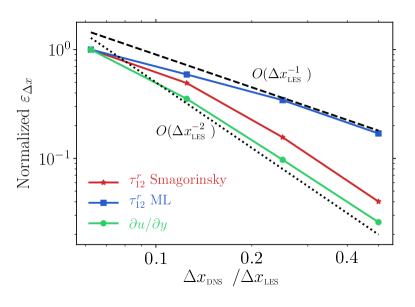
Figure 19: Relative difference $\varepsilon_{\Delta x}$ from (9.1) showing mesh dependence of $\tau^{r}_{12}$ for case A with $\overline{\Delta}=\Delta_{16}$ training for the indicated models (section 5.2). The corresponding convergence of $\partial u/\partial y$ is shown for reference.

In the sense of optimal LES[3], discrepancies between the formal convergence of unclosed LES solutions (or trusted DNS data) and the ideal closed LES solution are expected. The ideal LES closure, which achieves the upper limit of accuracy with respect to trusted data, must approximate Navier–Stokes physics that the filter operator (2.5) maps to its null space. These are, of course, not representable in an LES solution space even with explicit filtering[3].

Figure 19 may be understood in this context by considering an optimal closure model

$$\vec{\tau}\,^{r}_{\Delta x}=\mathrm{P}\vec{\tau}\,^{r}_{\mathrm{Ideal}}+\varepsilon_{\mathrm{P}}(\Delta x)+c\Delta x^{p},$$ (9.2)

where $\tau^{r}_{\mathrm{Ideal}}$ is the ideal LES closure model, $\mathrm{P}$ is a (non-unique) projection to the truncated $\Delta x$ LES solution space, $\varepsilon_{\mathrm{P}}(\Delta x)$ is the dynamical error in the Navier–Stokes solution due to the projection, and $c\Delta x^{p}$ is the spatial discretization error of the model inputs. Since $\mathrm{P}$ is linear and invertible, the relative difference (9.1) eliminates $\mathrm{P}\vec{\tau}\,^{r}_{\mathrm{Ideal}}$ leaving only the error terms. Traditional LES closures do not model $\varepsilon_{\mathrm{P}}(\Delta x)$ and so converge as $O(\Delta x^{p})$. Conversely, the a posteriori-trained (1.6) deep learning model does not, even though its inputs are $O(\Delta x^{p})$-accurate, which suggests that it at least partially accounts for $\varepsilon_{\mathrm{P}}(\Delta x)$.

9.2 Performance on out-of-sample meshes

The model is trained for a particular coarse resolution, for which, at least for established models, discretization errors are known to couple with model errors. The performance of the model suggests that it also compensates for discretization errors, which was assessed previously for isotropic turbulence.[11] Hence, it comes with no a priori assurance that it will be as accurate away from resolutions for which it was trained. We assess this by applying the $\mathbf{h}$ closure to finer grids than the training $\Delta_{16}$. Figure 20 shows the performance over a range of $\Delta_{N}$ using both instantaneous-velocity training and mean-statistics training. The instantaneous-velocity-trained model in figure 20 (a) reproduces the mean profile on $\Delta_{4}$ nearly as well as for the $\Delta_{16}$ trained case, but not so well on $\Delta_{8}$. The mean-flow training is more robust, as seen in figure 20 (b). However, the implicit filter definition used for a posteriori LES is still a potential source of error. The mean-flow training (figure 20b) is presumably less sensitive to discrepancies between this and the a priori explicit filter definition, although further testing is certainly warranted.

Finally, we note that a deep learning model trained only for isotropic turbulence[11] performed reasonably well when tested out-of-sample on the jet case A, although it was not as accurate as the deep learning models in figure 20. The model is at least stable and reasonably accurate when applied to different grids and potentially to different flows. However, its overall extrapolative capacity, for example, to different flow phenomena, is likely reduced.

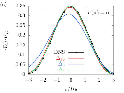
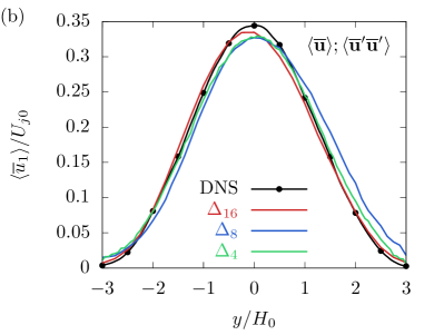
Figure 20: Predicted streamwise mean velocity for the single jet case (A) for grid-filter ratios $\overline{\Delta}/\Delta_{\text{{dns}}}$. (a) Instantaneous-velocity training; (b) mean-flow and Reynolds stress training. Both models were trained only on $\Delta_{16}$.

10 Additional Discussion

In some sense, it is unsurprising that a high-degree-of-freedom model can outperform established models with few if any parameters, at least for the modest degree of out-of-sample extrapolation we attempted here. However, determining viable parameters for this is challenging. The adjoint-based PDE-coupled training procedures used here seem to perform well for finding parameters sufficient for robust and extrapolative models. The predictive agreement with trusted data for coarse meshes is striking. Still, given the number of parameters required and the challenging optimization procedures needed, this should not be taken as an unqualified improvement. Indeed, a fair way to view results is recognition of just how well dynamic Smagorinsky, as an example of established models, does with neither significant parameterization nor a complicated training regimen. In closing, we revisit some of the motivations beyond the basic goal of increasing accuracy for fixed mesh resolution.

One particular hope is that this framework will facilitate representation of turbulence when it is coupled with additional physics, especially in cases where this coupling lacks models of the fidelity available for incompressible turbulence. The final demonstration, where the model is shown to also extrapolate to represent scalar mixing, is an example of this. Similarly, training of a robust model based only on mean statistics provides an avenue for predictions even when part of the physics (e.g., flame dynamics) might be insufficiently described to craft an explicit model. Generalizing high-degree-of-freedom models to out-of-sample flow conditions or new physics couplings is a main target for this procedure.

Even for inert incompressible turbulence, without the complexity of additional physics, we also anticipate potential synergies between the highly parameterized approach we introduce and established models and modeling approaches. Our efforts to interpret the successful neural-network model by fitting the parameters of low-degree-of-freedom models are a first step toward using the successful working representations to improve conventional models. A related opportunity is the use of a posteriori successful neural-network models to aid coefficient discovery in moderately-parameterized models, based on physical reasoning, such as those that aim to codify nonlinearly coupled multi-physical interactions. We anticipate a fruitful middle ground between fitting accuracy and generalization where the two modeling approaches can complement and augment each other.

An outstanding issue, which is shared with all turbulence sub-grid-scale modeling, is the interplay of numerical errors associated with the coarse mesh resolution and the model closures. As trained through solutions of the discrete flow equations and their adjoint, the current deep learning models account for errors introduced by the coarse discretizations, which is important for its predictive success. A potential drawback is that it risks linking the trained model with the specific mesh spacing (and discretization method) for which it is trained. In the present case, we demonstrated that this is not a severe limitation: the model is robustly predictive for different meshes, though accuracy is indeed reduced. Looking forward, it can be anticipated that systematically training for a range of mesh resolutions might provide improved predictions. We can also speculate that the training on the case A jet, which spreads by over a factor of two during the training period, might imbue the learned model with some robustness in this regard since it exposes the model to different nominal resolutions through the evolution of the flow. For example, if the development were exactly self-similar, then the model requirements for the $\Delta_{16}$ mesh at some later time would match those for the $\Delta_{8}$ mesh at the earlier time when the jet has half the later thickness. Systematic studies of extrapolative capacity to different resolutions, mesh configurations, numerical methods, and flows are all warranted.

Finally, it is important to address a general challenge faced when applying adjoint methods to turbulence. It is well-understood that the chaos of turbulence will, for long enough times, lead to divergence of sensitivity fields, which diminishes the utility of computed sensitivities. This is not a challenge for the short-time adjoint solutions used in the most of the present demonstrations, and we anticipate that many applications of this method will not suffer from this because of the character of the problem: a sub-grid-scale model to provide a stress correction for the local instantaneous resolved-scale turbulence. Since the large turbulence scales are relatively local in space and time, the sensitivity will not accumulate significantly. In general, however, this might limit applications with limited data availability, especially if it is sensitive to turbulence that is significantly distant in space and time. Further work will be required to understand how the Lyapunov divergence of turbulence might hinder the adjoint-based training. We do note that the adjoint equations remained sufficiently well-behaved when we trained and simulated over the entire time history of the jet flow when training for mean statistics.

Acknowledgments

This material is based in part upon work supported by the Department of Energy, National Nuclear Security Administration, under Award Number DE-NA0002374. This research is part of the Blue Waters sustained-petascale computing project, which is supported by the National Science Foundation (awards OCI-0725070 and ACI-1238993) and the State of Illinois. Blue Waters is a joint effort of the University of Illinois at Urbana–Champaign and its National Center for Supercomputing Applications.

References

- [1] C. Meneveau, J. Katz, Scale-invariance and turbulence models for large-eddy simulation, Annu. Rev. Fluid Mech. 32 (2000) 1–32.
- [2] S. Ghosal, Mathematical and physical constraints on large-eddy simulation of turbulence, AIAA J. 37 (4) (1999) 425–433.
- [3] J. A. Langford, R. D. Moser, Optimal LES formulations for isotropic turbulence, J. Fluid Mech. 398 (1999) 321–346.
- [4] M. Germano, U. Piomelli, P. Moin, W. H. Cabot, A dynamic subgrid-scale eddy viscosity model, Phys. Fluids 3 (7) (1991) 1760–1765.
- [5] D. K. Lilly, A proposed modification of the Germano subgrid-scale closure method, Phys. Fluids 4 (1992) 633–635.
- [6] B. Steiner, Z. DeVito, S. Chintala, S. Gross, A. Paszke, F. Massa, A. Lerer, G. Chanan, Z. Lin, E. Yang, A. Desmaison, A. Tejani, A. Kopf, J. Bradbury, L. Antiga, M. Raison, N. Gimelshein, S. Chilamkurthy, T. Killeen, L. Fang, J. Bai, Pytorch: An imperative style, high-performance deep learning library, NeurIPS 2019.
- [7] J. Ling, A. Kurzawski, J. Templeton, Reynolds averaged turbulence modelling using deep neural networks with embedded invariance, J. Fluid Mech. 807 (2016) 155–166.
- [8] M. Gamahara, Y. Hattori, Searching for turbulence models by artificial neural network, Phys. Rev. Fluids 2 (2017) 1–20.
- [9] A. Beck, D. Flad, C. D. Munz, Deep neural networks for data-driven LES closure models, J. Comp. Phys. 398 (2019) 108910.
- [10] M. P. Brenner, J. D. Eldredge, J. B. Freund, A perspective on machine learning for advancing fluid mechanics, Phys. Rev. Fluids 4 (2019) 100501.
- [11] J. Sirignano, J. F. MacArt, J. B. Freund, DPM: A deep learning PDE augmentation method with application to large-eddy simulation, J. Comp. Phys. 423 (2020) 109811.
- [12] J. R. Holland, J. D. Baeder, K. Duraisamy, Towards integrated field inversion and machine learning with embedded neural networks for RANS modeling, In: AIAA SciTech Forum (2019) 1884.
- [13] E. J. Parish, K. Duraisamy, A paradigm for data-driven predictive modeling using field inversion and machine learning, J. Comp. Phys. 305 (2016) 758–774.
- [14] G. Novati, H. L. de Laroussilhe, P. Koumoutsakos, Automating Turbulence Modeling by Multi-Agent Reinforcement Learning, arXiv:2005.09023 (2020) (preprint).
- [15] C. Rackauckas, Y. Ma, J. Martensen, C. Warner, K. Zubov, R. Supekar, D. Skinner, A. Ramadhan, A. Edelman, Universal Differential Equations for Scientific Machine Learning, arXiv:2001.04385 (2020) (preprint).
- [16] A. G. Baydin, B. A. Pearlmutter, A. A. Radul, J. M. Siskind, Automatic Differentiation in Machine Learning: a Survey, J. Mach. Learn. Res. 18 (2018) 1–43.
- [17] J. Smagorinsky, General circulation experiments with the primitive equations I. The basic experiment, Mon. Weather Rev. 91 (3) (1963) 99–164.
- [18] R. S. Rogallo, P. Moin, Numerical simulation of turbulent flows, Annu. Rev. Fluid Mech. 16 (1984) 99–137.
- [19] R. A. Clark, J. H. Ferziger, W. C. Reynolds, Evaluation of subgrid-scale models using a fully simulated turbulent flow, J. Fluid Mech. 91 (1) (1979) 1–16.
- [20] F. H. Harlow, J. E. Welch, Numerical calculation of time-dependent viscous incompressible flow of fluid with free surface, Phys. Fluids 8 (12) (1965) 2182–2189.
- [21] G.-S. Jiang, C.-W. Shu, Efficient implementation of weighted ENO schemes, J. Comput. Phys. 126 (1996) 202–228.
- [22] J. Kim, P. Moin, Application of a fractional-step method to incompressible Navier–Stokes equations, J. Comp. Phys. 59 (2) (1985) 308–323.
- [23] O. Desjardins, G. Blanquart, G. Balarac, H. Pitsch, High order conservative finite difference scheme for variable density low Mach number turbulent flows, J. Comp. Phys. 227 (15) (2008) 7125–7159.
- [24] J. B. Freund, S. K. Lele, P. Moin, Compressibility effects in a turbulent annular mixing layer. Part 2. Mixing of a passive scalar, J. Fluid Mech. 421 (2000) 269–292.
- [25] C. Pantano, S. Sarkar, A study of compressibility effects in the high-speed turbulent shear layer using direct simulation, J. Fluid Mech. 451 (2002) 329–371.
- [26] R. Knaus, C. Pantano, On the effect of heat release in turbulence spectra of non-premixed reacting shear layers, J. Fluid Mech. 626 (2009) 67–109.
- [27] E. R. Hawkes, O. Chatakonda, H. Kolla, A. R. Kerstein, J. H. Chen, A petascale direct numerical simulation study of the modelling of flame wrinkling for large-eddy simulations in intense turbulence, Combust. Flame 159 (2012) 2690–2703.
- [28] J. F. MacArt, T. Grenga, M. E. Mueller, Effects of combustion heat release on velocity and scalar statistics in turbulent premixed jet flames at low and high Karlovitz numbers, Combust. Flame 191 (2018) 468–485.
- [29] D. R. Miller, E. W. Comings, Force-momentum fields in a dual-jet flow, J. Fluid Mech. 7 (1960) 237–256.
- [30] X. Glorot, Y. Bengio, Understanding the difficulty of training deep feedforward neural networks, Proceedings of the thirteenth international conference on artificial intelligence and statistics (2010) 249–256.
- [31] I. Goodfellow, Y. Bengio, A. Courville, Deep Learning, MIT Press, 2016.
- [32] B. Vreman, B. J. Geurts, H. Kuerten, Large-eddy simulation of the temporal mixing layer using the Clark model, Theor. Comput. Fluid Dyn. 8 (1996) 309–324.
- [33] S. Banerjee, R. Krahl, F. Durst, C. Zenger, Presentation of anisotropy properties of turbulence, invariants versus eigenvalue approaches, J. Turbul. 8 (2007) N32.
- [34] J. O’Brien, C. A. Z. Towery, P. E. Hamlington, M. Ihme, A. Y. Poludnenko, J. Urzay, The cross-scale physical-space transfer of kinetic energy in turbulent premixed flames, Proc. Combust. Inst. 36 (2) (2017) 1967–1975.
- [35] J. F. MacArt, M. E. Mueller, Scaling and modeling of heat-release effects on subfilter turbulence in premixed combustion, Center for Turbulence Research Proceedings of the Summer Program (2018) 299–308.
- [36] J. F. MacArt, M. E. Mueller, Semi-implicit iterative methods for low Mach number turbulent reacting flows: Operator splitting versus approximate factorization, J. Comp. Phys. 326 (2016) 569–595.