Initialization and Regularization of
Factorized Neural Layers

Abstract

Factorized layers—operations parameterized by products of two or more matrices—occur in a variety of deep learning contexts, including compressed model training, certain types of knowledge distillation, and multi-head self-attention architectures. We study how to initialize and regularize deep nets containing such layers, examining two simple, understudied schemes, spectral initialization and Frobenius decay, for improving their performance. The guiding insight is to design optimization routines for these networks that are as close as possible to that of their well-tuned, non-decomposed counterparts; we back this intuition with an analysis of how the initialization and regularization schemes impact training with gradient descent, drawing on modern attempts to understand the interplay of weight-decay and batch-normalization. Empirically, we highlight the benefits of spectral initialization and Frobenius decay across a variety of settings. In model compression, we show that they enable low-rank methods to significantly outperform both unstructured sparsity and tensor methods on the task of training low-memory residual networks; analogs of the schemes also improve the performance of tensor decomposition techniques. For knowledge distillation, Frobenius decay enables a simple, overcomplete baseline that yields a compact model from over-parameterized training without requiring retraining with or pruning a teacher network. Finally, we show how both schemes applied to multi-head attention lead to improved performance on both translation and unsupervised pre-training.

1 Introduction

Most neural network layers consist of matrix-parameterized functions followed by simple operations such as activation or normalization. These layers are the main sources of model expressivity, but also the biggest contributors to computation and memory cost; thus modifying these layers to improve computational performance while maintaining performance is highly desirable. We study the approach of factorizing layers, i.e. reparameterizing them so that their weights are defined as products of two or more matrices. When these are smaller than the original matrix, the resulting networks are more efficient for both training and inference (Denil et al., 2013; Moczulski et al., 2015; Ioannou et al., 2016; Tai et al., 2016), resulting in model compression. On the other hand, if training cost is not a concern, one can increase the width or depth of the factors to over-parameterize models (Guo et al., 2020; Cao et al., 2020), improving learning without increasing inference-time cost. This can be seen as a simple, teacher-free form of knowledge distillation. Factorized layers also arise implicitly, such as in the case of multi-head attention (MHA) (Vaswani et al., 2017).

Despite such appealing properties, networks with factorized neural layers are non-trivial to train from scratch, requiring custom initialization, regularization, and optimization schemes. In this paper we focus on initialization, regularization, and how they interact with gradient-based optimization of factorized layers. We first study spectral initialization (SI), which initializes factors using singular value decomposition (SVD) so that their product approximates the target un-factorized matrix. Then, we study Frobenius decay (FD), which regularizes the product of matrices in a factorized layer rather than its individual terms. Both are motivated by matching the training regimen of the analogous un-factorized optimization. Note that SI has been previously considered in the context of model compression, albeit usually for factorizing pre-trained models (Nakkiran et al., 2015; Yaguchi et al., 2019; Yang et al., 2020) rather than low-rank initialization for end-to-end training; FD has been used in model compression using an uncompressed teacher (Idelbayev & Carreira-Perpiñán, 2020).

We formalize and study the justifications of SI and FD from both the classical perspective—matching the un-factorized objective and scaling—and in the presence of BatchNorm (Ioffe & Szegedy, 2015), where this does not apply. Extending recent studies of weight-decay (Zhang et al., 2019), we argue that the effective step-size at spectral initialization is controlled by the factorization’s Frobenius norm and show convincing evidence that weight-decay penalizes the nuclear norm.

We then turn to applications, starting with low-memory training, which is dominated by unstructured sparsity methods—i.e. guessing “lottery tickets” (Frankle & Carbin, 2019)—with a prevailing trend of viewing low-rank methods as uncompetitive for compression (Blalock et al., 2020; Zhang et al., 2020; Idelbayev & Carreira-Perpiñán, 2020; Su et al., 2020). Here we show that, without tuning, factorized neural layers outperform all structured sparsity methods on ResNet architectures (He et al., 2016), despite lagging on VGG (Simonyan & Zisserman, 2015). Through ablations, we show that this result is due to using both SI and FD on the factorized layers. We further compare to a recent evaluation of tensor-decomposition approaches for compressed WideResNet training (Zagoruyko & Komodakis, 2016; Gray et al., 2019), showing that (a) low-rank approaches with SI and FD can outperform them and (b) they are themselves helped by tensor-variants of SI and FD.

We also study a fledgling subfield we term overcomplete knowledge distillation (Arora et al., 2018; Guo et al., 2020; Cao et al., 2020) in which model weights are over-parameterized as overcomplete factorizations; after training the factors are multiplied to obtain a compact representation of the same network. We show that FD leads to significant improvements, e.g. we outperform ResNet110 with an overcomplete ResNet56 that takes 1.5x less time to train and has 2x fewer parameters at test-time.

Finally, we study Transformer architectures, starting by showing that FD improves translation performance when applied to MHA. We also show that SI is critical for low-rank training of the model’s linear layers. In an application to BERT pre-training (Devlin et al., 2019), we construct a Frobenius-regularized variant—FLAMBé—of the LAMB method (You et al., 2020), and show that, much like for transformers, it improves performance both for full-rank and low-rank MHA layers.

To summarize, our main contributions are (1) motivating the study of training factorized layers via both the usual setting (model compression) and recent applications (distillation, multi-head attention), (2) justifying the use of SI and FD mathematically and experimentally, and (3) demonstrating their effectiveness by providing strong baselines and novel advances in many settings. Code to reproduce our results is available here: https://github.com/microsoft/fnl_paper.

1.1 Related Work

We are not the first study gradient descent on factorized layers; in particular, deep linear nets are well-studied in theory (Saxe et al., 2014; Gunasekar et al., 2019). Apart from Bernacchia et al. (2018) these largely examine existing algorithms, although Arora et al. (2018) do effectively propose overcomplete knowledge distillation. Rather than the descent method, we focus on the initialization and regularization. For the former, several papers use SI after training (Nakkiran et al., 2015; Yaguchi et al., 2019; Yang et al., 2020), while Ioannou et al. (2016) argue for initializing factors as though they were single layers, which we find inferior to SI in some cases. Outside deep learning, spectral methods have also been shown to yield better initializations for certain matrix and tensor problems (Keshavan et al., 2010; Chi et al., 2019; Cai et al., 2019). For regularization, Gray et al. (2019) suggest compression-rate scaling (CRS), which scales weight-decay using the reduction in parameter count; this is justified via the usual Bayesian understanding of $\ell_{2}$-regularization (Murphy, 2012). However, we find that FD is superior to any tuning of regular weight-decay, which subsumes CRS. Our own analysis is based on recent work suggesting that the function of weight-decay is to aid optimization by preventing the effective step-size from becoming too small (Zhang et al., 2019).

2 Preliminaries on Factorized Neural Layers

In the training phase of (self-)supervised ML, we often solve optimization problems of the form $\min_{\theta\in\Theta}\frac{1}{|{\mathcal{S}}|}\sum_{({\bm{x}},{\bm{y}})\in{\mathcal{S}}}\ell(f_{\theta}({\bm{x}}),{\bm{y}})+\Omega(\theta)$, where $f_{\theta}:{\mathcal{X}}\mapsto{\mathcal{Y}}$ is a function from input domain ${\mathcal{X}}$ to output domain ${\mathcal{Y}}$ parameterized by elements $\theta\in\Theta$, $\ell:{\mathcal{Y}}\times{\mathcal{Y}}\mapsto\mathbb{R}$ is a scalar-valued loss function, $\Omega:\Theta\mapsto\mathbb{R}$ is a scalar-valued regularizer, and ${\mathcal{S}}\subset{\mathcal{X}}\times{\mathcal{Y}}$ is a finite set of (self-)supervised training examples. We study the setting where $f_{\theta}$ is a neural network, an $L$-layer function whose parameters $\theta$ consist of $L$ matrices ${\bm{W}}_{i}\in\mathbb{R}^{m_{i}\times n_{i}}$ and whose output $f_{\theta}({\bm{x}})$ given input ${\bm{x}}$ is defined recursively using $L$ functions $g_{i}$ via the formula ${\bm{x}}_{i}=g_{i}({\bm{W}}_{i},{\bm{x}}_{i-1})$, with ${\bm{x}}_{0}={\bm{x}}$ and $f_{\theta}({\bm{x}})={\bm{x}}_{L}$.

The standard approach to training $f_{\theta}$ is to specify the regularizer $\Omega$, (randomly) pick an initialization in $\Theta$, and iteratively update the parameters using some first-order algorithm such as SGD to optimize the objective above until some stopping criterion is met. However, in many cases we instead optimize over factorized variants of these networks, in which some or all of the matrices ${\bm{W}}_{i}\in\mathbb{R}^{m_{i}\times n_{i}}$ are re-parameterized as a product ${\bm{W}}_{i}={\bm{U}}_{i}(\prod_{j=1}^{d_{i}}{\bm{M}}_{ij}){\bm{V}}_{i}^{T}$ for some inner depth $d_{i}\geq 0$ and matrices ${\bm{U}}_{i}\in\mathbb{R}^{m_{i}\times r_{i}},{\bm{V}}_{i}\in\mathbb{R}^{n_{i}\times r_{i}}$, and ${\bm{M}}_{ij}\in\mathbb{R}^{r_{i}\times r_{i}}~{}\forall~{}j$. As discussed in the following examples, this can be done to obtain better generalization, improve optimization, or satisfy practical computational or memory constraints during training or inference. For simplicity, we drop the subscript $i$ whenever re-parameterizing only one layer and only consider the cases when inner depth $d$ is 0 or 1.

2.1 Fully-Connected Layers

A fully-connected layer takes an $n$-dimensional input ${\bm{x}}_{i-1}$ and outputs an $m$-dimensional vector ${\bm{x}}_{i}=\sigma({\bm{W}}{\bm{x}}_{i-1})$, where $\sigma:\mathbb{R}^{m}\mapsto\mathbb{R}^{m}$ is an element-wise activation function. Here, decomposing ${\bm{W}}\in\mathbb{R}^{m\times n}$ into the product ${\bm{U}}{\bm{V}}^{T}$, where ${\bm{U}}\in\mathbb{R}^{m\times r},{\bm{V}}\in\mathbb{R}^{n\times r}$, and setting $r\ll\min\{m,n\}$ reduces computation and memory costs from ${\mathcal{O}}(mn)$ to ${\mathcal{O}}(mr+nr)$. We refer to this setting as model compression. Standard learning theory suggests that a small rank $r$ also improves generalization, e.g. for a factorized fully-connected ReLU network, applying $\|{\bm{W}}\|_{F}^{2}/\|{\bm{W}}\|_{2}^{2}\leq\operatorname{rank}({\bm{W}})$ to Neyshabur et al. (2018, Theorem 1) and substituting ${\bm{W}}_{i}={\bm{U}}_{i}{\bm{V}}_{i}^{T}$ gives a w.h.p. margin-bound $\tilde{\mathcal{O}}(\sqrt{mr/|{\mathcal{S}}|})$ suggesting that generalization error varies with the square root of the rank (see Corollary A.1).

Alternatively, by setting $r\geq\min\{m,n\}$ and/or including an inner matrix ${\bm{M}}\in\mathbb{R}^{r\times r}$, we can attempt to take advantage of improved optimization due to increased width (Du & Hu, 2019) and/or increased depth (Arora et al., 2018). Crucially, this does not increase inference costs because we can recompose the matrix after training and just use the product. As the goal is to obtain a better small model by first training a large one, we refer to this setting as overcomplete knowledge distillation; of course, unlike regular distillation it is much simpler since there is no student-teacher training stage.

2.2 Convolutional Layers

A 2d convolutional layer takes an $h\times w\times c_{i-1}$-dimensional input ${\bm{x}}_{i-1}$ and outputs a $h\times w\times c_{i}$-dimensional output ${\bm{x}}_{i}$ defined by convolving $c_{i}$ different $k\times k$ filters over each of $c_{i-1}$ input channels. Often the result is passed through a nonlinearity. 2d convolutional layers are parameterized by $c_{i}\times c_{i-1}\times k\times k$ tensors and require $O(k^{2}c_{i}c_{i-1})$ memory and compute. A straightforward way of factorizing this tensor without using tensor decomposition is to reshape it into a $c_{i}k\times c_{i-1}k$ matrix ${\bm{W}}$, which can then be decomposed as ${\bm{W}}={\bm{U}}{\bm{V}}^{T}$ for ${\bm{U}}\in\mathbb{R}^{c_{i}k\times r}$, ${\bm{V}}\in\mathbb{R}^{c_{i-1}k\times r}$ and some rank $r>0$. As in the fully-connected case, we can either set the rank $r$ to be small in order to reduce the number of parameters or alternatively increase the width ($r$) or the depth ($d$) of the factorization to do overcomplete knowledge distillation.

Note that in the low-rank case a naive approach does not save computation since we must first multiply ${\bm{U}}$ and ${\bm{V}}^{T}$, reshape the product ${\bm{U}}{\bm{V}}^{T}$, and then use the resulting tensor in a regular 2d convolution of the original size and complexity. However, as shown by Tai et al. (2016), applying the 2d $k\times k$ convolution with $c_{i-1}$ input channels and $c_{i}$ output channels obtained by reshaping ${\bm{U}}{\bm{V}}^{T}$ is equivalent to a composition of two 1d convolutions: the first defined by ${\bm{V}}^{T}\in\mathbb{R}^{r\times c_{i-1}k}$ consists of $r$ output channels and filters of size $k$ along one input dimension and the second defined by ${\bm{U}}\in\mathbb{R}^{c_{i}k\times r}$ consists of $c_{i}$ output channels and filters of size $k$ along the other input dimension. Together the two 1d convolutions require $O(kr(c_{i}+c_{i-1}))$ memory and computation, which is significantly better than the $O(k^{2}c_{i}c_{i-1})$ cost of the unfactorized case if $r\ll k\min\{c_{i},c_{i-1}\}$.

2.3 Multi-Head Attention

An MHA layer (Vaswani et al., 2017) with $H$ attention heads and hidden dimension $d$ can be expressed as being parameterized with $4H$ matrices: one each of ${\bm{Q}}_{h},{\bm{K}}_{h},{\bm{V}}_{h},{\bm{O}}_{h}\in\mathbb{R}^{d\times d/H}$ for each head $h$. Then for a length-$T$ input ${\bm{x}}\in\mathbb{R}^{T\times d}$ it outputs

$$\sum_{h=1}^{H}\operatorname{Softmax}\left(\frac{{\bm{x}}{\bm{Q}}_{h}{\bm{K}}_{h}^{T}{\bm{x}}^{T}}{\sqrt{d/H}}\right){\bm{x}}{\bm{V}}_{h}{\bm{O}}_{h}^{T}\vspace{-1mm}$$ (1)

MHA combines $2H$ quadratic forms ${\bm{Q}}_{h}{\bm{K}}_{h}^{T}$, ${\bm{V}}_{h}{\bm{O}}_{h}^{T}$ of rank $r=d/H$, each a product of matrices, i.e. a factorized layer. We refer to the first form as “Query-Key” and the second as “Output-Value.” Note that $r$ can be varied independently of $d$ to change expressivity, memory, and computation.

3 Initialization and Regularization

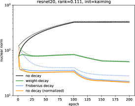
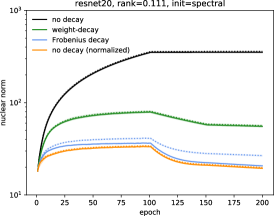
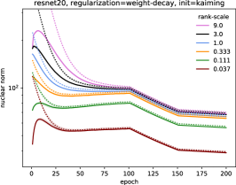
Figure 1: Average nuclear norm across factorized layers of ResNet20 during CIFAR-10 training when initialized regularly (left) and using SI (center); the dotted line is the upper bound on the nuclear norm regularized by weight-decay (2). The right plot track the same quantities for the case of regular weight-decay across different rank-scales. “no decay (normalized)” normalizes matrix factors after each step to have the same norm as “Frobenius decay ” (detailed in Section 3.3).

We now define the initialization and regularization schemes we study as natural extensions of techniques for non-factorized models. They thus require no tuning when an existing training implementation of a non-factorized deep net is available. We later discuss how to justify these schemes when layers are normalized, e.g. using BatchNorm (Ioffe & Szegedy, 2015). In all experiments with convolutional models in this and subsequent sections we factorize all layers except the first and last, which are small, and determine layer ranks by multiplying a uniform scaling factor by the product of a layer’s output channels and kernel width. This rank-scale can be varied to attain the desired number of parameters. Note that our approach may be further improved via a more sophisticated or adaptive rank-assignment scheme (Idelbayev & Carreira-Perpiñán, 2020).

3.1 Spectral Initialization

Initialization is a major focus of deep learning research (He et al., 2015; Mishkin & Matas, 2016; Yang & Schoenholz, 2017). A common approach is to prevent compounding changes in the norms of the intermediate representations across layers caused by repeated multiplication by the weight matrices. The spectral initialization scheme for initializing low-rank factorized layers attempts to inherit, when possible, this property from an existing initialization by using SVD to ensure that the resulting product matrix is as close as possible to the original parameter:

Definition 3.1.

Let ${\bm{W}}\in\mathbb{R}^{m\times n}$ be a parameter of an unfactorized layer. For $r\leq\min\{m,n\}$ the spectral initialization (SI) of the factors ${\bm{U}}\in\mathbb{R}^{m\times r},{\bm{V}}\in\mathbb{R}^{n\times r}$ of the corresponding factorized layer sets ${\bm{U}}=\tilde{\bm{U}}\sqrt{\Sigma}$ and ${\bm{V}}=\tilde{\bm{V}}\sqrt{\Sigma}$, for $\tilde{\bm{U}},\Sigma,\tilde{\bm{V}}=\operatorname{SVD}_{r}({\bm{W}})$ given by the rank-$r$ SVD of ${\bm{W}}$.

SI preserves the largest singular value of ${\bm{W}}$, so if the original scheme did not suffer from a compounding increase in representation norm then neither will spectral initialization. On the other hand, while low-rank layers impose a nullspace, SI aligns it with the directions minimized by ${\bm{W}}$.

3.2 Frobenius Decay

Weight-decay is a common regularizer for deep nets, often implemented explicitly by adding $\Omega(\theta)=\frac{\lambda}{2}\sum_{{\bm{W}}\in\theta}\|{\bm{W}}\|_{F}^{2}$ to the objective for some $\lambda\geq 0$. Classically, it is thought to improve generalization by constraining model capacity. When training factorized layers parameterized by ${\bm{U}}(\prod_{j=1}^{d}{\bm{M}}_{j}){\bm{V}}^{T}$, the easiest approach to implement is to replace each $\frac{\lambda}{2}\|{\bm{W}}\|_{F}^{2}$ term in $\Omega(\theta)$ by $\frac{\lambda}{2}\left(\|{\bm{U}}\|_{F}^{2}+\|{\bm{V}}\|_{F}^{2}+\sum_{j=1}^{d}\|{\bm{M}}_{j}\|_{F}^{2}\right)$. However, this yields a very different optimization problem: for example, if we consider the case of $d=0$ then this regularizer is in fact an upper bound on the nuclear norm of the recomposed matrix ${\bm{U}}{\bm{V}}^{T}$ (Srebro & Shraibman, 2005, Lemma 1):

$$\frac{\lambda}{2}\left(\|{\bm{U}}\|_{F}^{2}+\|{\bm{V}}\|_{F}^{2}\right)\geq\min_{\tilde{\bm{U}}\tilde{\bm{V}}^{T}={\bm{U}}{\bm{V}}^{T}}\frac{\lambda}{2}\left(\|\tilde{\bm{U}}\|_{F}^{2}+\|\tilde{\bm{V}}\|_{F}^{2}\right)=\lambda\|{\bm{U}}{\bm{V}}^{T}\|_{\ast}\vspace{-1mm}$$ (2)

In fact, Figure 1 shows that for weight-decay this upper bound is tight throughout the training of factorized ResNet20 across a variety of ranks and initializations, suggesting that the naive approach is indeed regularizing the nuclear norm rather than the Frobenius norm.

Since compression already constrains capacity, in the low-rank case one might favor just reducing regularization, e.g. multiplying $\lambda$ by the compression rate (Gray et al., 2019). However, Figure 2 shows that this can lead to worse performance, and the approach still penalizes the nuclear norm. Frobenius decay avoids this issue by simply penalizing the squared norm of the entire factorization:

Definition 3.2.

For $\lambda\geq 0$ let $\frac{\lambda}{2}\|{\bm{W}}\|_{F}^{2}$ be the contribution of an unfactorized layer parameterized by ${\bm{W}}\in\mathbb{R}^{m\times n}$ to the penalty term. Then the Frobenius decay (FD) penalty on matrices ${\bm{U}}\in\mathbb{R}^{m\times r}$, ${\bm{V}}\in\mathbb{R}^{n\times r}$, and ${\bm{M}}_{j}\in\mathbb{R}^{r\times r}$ of the corresponding factorized layer is $\frac{\lambda}{2}\left\|{\bm{U}}(\prod_{j=1}^{d}{\bm{M}}_{j}){\bm{V}}^{T}\right\|_{F}^{2}$.

By substituting the factorization directly, FD makes the least change to the problem: rank-$r$ optima of the non-factorized objective will also minimize the factorized one. We can also bound generalization error of the ReLU net from Section 2.1 by a term $\tilde{\mathcal{O}}\left(\sqrt{\frac{m}{|{\mathcal{S}}|}\sum_{i=1}^{L}\|{\bm{U}}_{i}(\prod_{j=1}^{d}{\bm{M}}_{ij}){\bm{V}}_{i}^{T}\|_{F}^{2}}\right)$ varying directly with the quantity penalized by FD (see Corollary A.2). Notably, FD is a stronger penalty than the nuclear norm implicitly regularized by weight-decay, yet it still yields better models.

3.3 Initialization and Regularization in the Presence of Normalization

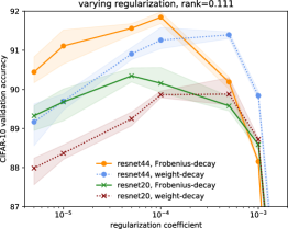
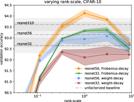
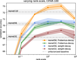
Figure 2: Comparison of weight-decay and FD at different regularization levels (left) and different rank-scales (center and right) when training factorized ResNets on CIFAR.

The use of spectral initialization and Frobenius decay is largely motivated by the norms of the recomposed matrices: SI prevents them increasing feature vector norms across layers, while FD constrains model capacity via parameter norms. However, normalization layers like BatchNorm (Ioffe & Szegedy, 2015) and others (Ba et al., 2016) largely negate the forward-pass and model-capacity effects of the norms of the weights parameterizing the layers they follow. Thus for most modern models we need a different explanation for the effectiveness of SI and FD.

Despite the fact that most layers’ norms do not affect inference or capacity, weight-decay remains useful for optimizing deep nets. Recently, Zhang et al. (2019) extended the analysis of Hoffer et al. (2018) to argue that the effective step-size of the weight direction $\hat{\bm{W}}$ is roughly $\eta/\|{\bm{W}}\|_{F}^{2}$, where $\eta$ is the SGD step-size. Thus by preventing the norm of ${\bm{W}}$ from growing too large weight-decay maintains a large-enough effective step-size during training. We draw on this analysis to explore the effect of SI and FD on factorized models. For simplicity, we define a normalized layer to be one that does not depend on the scale of its parameter. Ignoring stability offset terms, this definition roughly holds for normalized linear layers, convolutional layers in ResNets, and the Output-Value quadratic form in Transformers if the residual connection is added after rather than before normalization.

Definition 3.3.

A normalized layer $g({\bm{W}},{\bm{x}})$ parameterized by ${\bm{W}}\in\mathbb{R}^{m\times n}$ is one that satisfies $g({\bm{W}},{\bm{x}})=g(\rho{\bm{W}},{\bm{x}})$ for all ${\bm{W}}\in\mathbb{R}^{m\times n}$ and all positive scalars $\rho$.

Because the output does not depend on the magnitude of ${\bm{U}}{\bm{V}}^{T}$, what matters is the direction of the composed matrix. During an SGD step this direction is updated as follows (proof in Appendix B):

Claim 3.1.

At all steps $t\geq 0$ let $g$ be a normalized layer of a differentiable model $f_{\theta_{t}}:{\mathcal{X}}\mapsto{\mathcal{Y}}$ parameterized by ${\bm{U}}_{t}{\bm{V}}_{t}^{T}$ for ${\bm{U}}_{t}\in\mathbb{R}^{m\times r},{\bm{V}}_{t}^{T}\in\mathbb{R}^{n\times r}$, $r\geq 1$. Suppose we update ${\bm{P}}={\bm{U}}$ and ${\bm{P}}={\bm{V}}$ by SGD, setting ${\bm{P}}_{t+1}\leftarrow{\bm{P}}_{t}-\eta\nabla_{{\bm{P}}_{t}}$ using a gradient $\nabla_{{\bm{P}}_{t}}=\frac{1}{|{\mathcal{B}}|}\sum_{({\bm{x}},{\bm{y}})\in{\mathcal{B}}}\nabla_{{\bm{P}}_{t}}\ell(f_{\theta_{t}}({\bm{x}}),{\bm{y}})$ over batch ${\mathcal{B}}\subset({\mathcal{X}},{\mathcal{Y}})$ and $\eta>0$ sufficiently small. Then for $\hat{\nabla}_{t}=\nabla_{\hat{\bm{W}}_{t}}{\bm{V}}_{t}{\bm{V}}_{t}^{T}+{\bm{U}}_{t}{\bm{U}}_{t}^{T}\nabla_{\hat{\bm{W}}_{t}}$ we have that the vectorized direction $\hat{\bm{w}}_{t}=\operatorname{vec}(\hat{\bm{W}}_{t})$ of ${\bm{W}}_{t}={\bm{U}}_{t}{\bm{V}}_{t}^{T}$ is updated as

$$\hat{\bm{w}}_{t+1}\leftarrow\hat{\bm{w}}_{t}-\frac{\eta}{\|{\bm{W}}_{t}\|_{F}^{2}}\left({\bm{I}}_{mn}-\hat{\bm{w}}_{t}\hat{\bm{w}}_{t}^{T}\right)\operatorname{vec}(\hat{\nabla}_{t})+{\mathcal{O}}(\eta^{2})\vspace{-1mm}$$ (3)

Note that (1) we ignore decay because $\lambda={\mathcal{O}}(\eta)$ so any resulting term is ${\mathcal{O}}(\eta^{2})$ and (2) the update rule is almost the same as that obtained for the unfactorized case by Zhang et al. (2019), except they have $\hat{\nabla}_{t}$ as the true gradient of the direction. Thus, apart from a rank-one correction, $\hat{\bm{W}}_{t}$ is approximately updated with step-size $\eta/\|{\bm{W}}_{t}\|_{F}^{2}$ multiplying a sum $\hat{\nabla}_{t}$ of two positive semi-definite linear transformations of its gradient $\nabla_{\hat{\bm{W}}_{t}}$. Note that, in the special case where the factorization is full-rank, this means that $\hat{\nabla}_{t}$ is close to a scalar multiple of $\nabla_{\hat{\bm{W}}_{t}}$ if the singular values are very similar. If ${\bm{W}}$ is a Gaussian ensemble with scale $1/\sqrt{n}$, which roughly aligns with common initialization schemes (He et al., 2015), then its singular values are roughly distributed around 1 and supported on $[0,2]$ (Bai & Yin, 1993), and so the linear transforms will not significantly increase the magnitude of $\nabla_{\hat{\bm{W}}_{t}}$. In the following discussion, we treat $\left({\bm{I}}_{mn}-\hat{\bm{w}}_{t}\hat{\bm{w}}_{t}^{T}\right)\operatorname{vec}(\hat{\nabla}_{t})$ as the effective gradient update for the refactorized parameter $\hat{\bm{w}}$.

As in the unfactorized case, our analysis suggests that, the main role of decay may be to maintain a large effective learning rate $\eta/\|{\bm{W}}\|_{F}^{2}$; furthermore, FD may be more effective than regular decay because it provides stronger regularization and directly penalizes the quantity of interest. We support this hypothesis using experiments analogous to Zhang et al. (2019) by comparing training a low-rank ResNet-20 with FD to training it with no decay but at each step normalizing all BatchNormed layers to have the same Frobenius norm as the FD run. In Figure 3 we see that the latter scheme closely tracks the former in terms of both the training loss and the test accuracy. Figure 3 also shows that FD maintains a higher effective step-size than regular weight-decay throughout training.

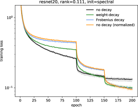
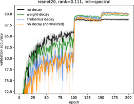
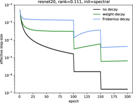
Figure 3: Traces depicting training of low-rank ResNet-20 with different decay settings; “no decay (normalized)” normalizes matrix factors after each step to have the same norm as “Frobenius decay.” The effective step size (right) is the average over convolution layers $i$ of $\eta/\|{\bm{U}}_{i}{\bm{V}}_{i}^{T}\|_{F}^{2}$.

4 Compressed Model Training: Low-Rank, Sparse, and Tensorial

Table 1: Comparison of low-rank and sparse training in a common evaluation setting for “ticket-guessing” (Wang et al., 2020; Su et al., 2020). Best results overall are italicized; best results from full low-memory training are bolded. For complete results and deviations see Tables 5 and 6.

	VGG19${}^{\textrm{NFC}}$ (full model)⋆	CIFAR-10 (93.75$\pm$0.48)			CIFAR-100 (73.42$\pm$0.17)			Tiny-ImageNet (62.19$\pm$0.74)
Regime	Compressed (from $\approx$20M)	0.10	0.05	0.02	0.10	0.05	0.02	0.10	0.05	0.02
Regular	Pruning∗	93.83	93.69	93.49	73.83	73.07	71.69	61.21	60.49	55.55
Training	Lottery† (w. hybrid/rewind)	94.14	93.99	93.52	74.06	73.10	71.61	61.19	60.57	56.18
Low Memory Training	Dynamic Sparsity‡	93.75	93.86	93.13	72.36	71.98	70.70	62.49	59.81	58.36
	Fixed Sparsity#	93.77	93.43	92.45	72.84	71.83	68.98	61.02	59.50	57.28
	Low-Rank⋆	90.71	88.08	80.81	62.32	54.97	42.80	48.50	46.98	36.57
	Low-Rank (SI)⋆	90.99	88.61	82.53	63.77	58.51	45.02	49.87	46.73	37.25
	Low-Rank (FD)⋆	91.57	88.16	82.81	64.07	59.34	45.73	53.93	47.95	35.63
	Low-Rank (SI & FD)⋆	91.58	88.98	83.27	65.61	60.1	46.43	53.53	47.60	35.68
	ResNet32${}^{\textrm{x2}}$ (full model)⋆	CIFAR-10 (94.49$\pm$0.29)			CIFAR-100 (75.41$\pm$1.26)			Tiny-ImageNet (63.02$\pm$0.94)
Regime	Compressed (from $\approx$7.5M)	0.10	0.05	0.02	0.10	0.05	0.02	0.15	0.10	0.05
Regular	Pruning∗	94.21	93.29	90.31	72.34	68.73	60.65	58.86	57.62	51.70
Training	Lottery† (w. hybrid/rewind)	94.14	93.02	90.85	72.41	69.28	63.44	60.31	57.77	51.21
Low Memory Training	Dynamic Sparsity‡	92.97	91.61	88.46	69.66	68.20	62.25	57.08	57.19	56.18
	Fixed Sparsity#	92.97	91.60	89.10	69.70	66.82	60.11	57.25	55.53	51.41
	Low-Rank⋆	93.59	92.45	87.95	72.71	67.86	61.08	60.82	58.72	55.39
	Low-Rank (SI)⋆	92.52	91.72	87.36	71.71	67.41	60.79	59.53	57.60	55.00
	Low-Rank (FD)⋆	92.92	89.44	83.05	71.85	66.89	55.31	59.45	57.24	54.15
	Low-Rank (SI & FD)⋆	94.34	92.90	87.97	74.41	70.22	61.40	62.24	60.25	55.97

• Best of (LeCun et al., 1990; Zeng & Urtasun, 2019), obtained from Wang et al. (2020).

• Best of (Frankle & Carbin, 2019; Renda et al., 2020; Su et al., 2020), obtained from Wang et al. (2020) and Su et al. (2020).

• Best of (Mostafa & Wang, 2019; Mocanu et al., 2018; Bellec et al., 2018), obtained from Wang et al. (2020).

• Best of (Lee et al., 2018; Wang et al., 2020; Su et al., 2020), obtained from Wang et al. (2020) and Su et al. (2020).

• Our method or our reproduction; results averaged over three random trials.

We first study SI and FD for training factorized models with low-rank convolutional layers, comparing against the dominant approaches to low-memory training: sparse layers and tensor decomposition. For direct comparison we evaluate models with near-identical parameter counts; note that by normalizing by memory we disadvantage the low-rank approach, which often has a comparative advantage for speed. All models are trained for 200 epochs with the same optimizer settings as for the unfactorized models; the weight-decay coefficient is left unchanged when replacing by FD.

Low-Rank and Sparse Training:

We train modified ResNet32 and VGG19 used in the lottery-ticket-guessing literature (Wang et al., 2020; Su et al., 2020). Motivated by Frankle & Carbin (2019), such methods fix a sparsity pattern at initialization and train only the unpruned weights. While they achieve high parameter savings, their computational advantages over full models are less clear, as software and accelerators often do not efficiently implement arbitrary sparsity (Paszke et al., 2019; NVIDIA, 2020). In contrast, we do see acceleration via low-rank convolutions, almost halving the time of ResNet’s forward and backward pass at the highest compression. For completeness, we also show methods that vary the sparsity pattern (dynamic), prune trained models (pruning), and prune trained models and retrain (lottery); note that the latter two require training an uncompressed model.

In Table 1 we see that the low-rank approach, with SI & FD, dominates at the higher memory settings of ResNet across all three datasets considered, often outperforming even approaches that train an uncompressed model first. It is also close to the best compressed training approach in the lowest memory setting for CIFAR-100 (Krizhevksy, 2009) and Tiny-ImageNet (Deng et al., 2009). On the other hand, the low-rank approach is substantially worse for VGG; nevertheless, ResNet is both smaller and more accurate, so if the goal is an accurate compressed model learned from scratch then one should prefer the low-rank approach. Our results demonstrate a strong, simple baseline not frequently compared to in the low-memory training literature (Frankle & Carbin, 2019; Wang et al., 2020; Su et al., 2020). In fact, since it preserves the top singular components of the original weights, SI can itself be considered a type of (spectral) magnitude pruning. Finally, Table 1 highlights the complementary nature of SI and FD, which outperform regular low-rank training on both models, although interestingly they consistently decrease ResNet performance when used separately.

Matrix and Tensor Decomposition:

Table 2: Comparison of low-rank and tensor-decomposition training of WideResNet28-10 on CIFAR-10 (mean of 3 trials) with different regularization and initialization. Best errors bolded.

compression	decomposition∗	WD†	WD† & SI	CRS‡	CRS‡ & SI	FD	FD & SI
none ($\approx$36.5M param.)		3.21$\pm$0.22
0.01667	Low-Rank	7.62$\pm$0.08	7.72$\pm$0.11	8.63$\pm$0.87	8.83$\pm$0.17	7.23$\pm$0.32	7.26$\pm$0.45
($\approx$0.61M param.)	Tensor-Train	8.55$\pm$4.22	7.72$\pm$0.46	7.01$\pm$0.35	6.52$\pm$0.17	7.26$\pm$0.73	6.22$\pm$0.50
0.06667	Low-Rank	5.31$\pm$0.06	5.49$\pm$0.42	5.86$\pm$0.22	5.53$\pm$0.72	3.89$\pm$0.17	3.86$\pm$0.22
($\approx$2.4M param.)	Tensor-Train	7.33$\pm$0.27	6.49$\pm$0.30	5.20$\pm$0.37	4.79$\pm$0.15	5.02$\pm$0.15	5.10$\pm$0.35

• See Table 7 for results using the Tucker decomposition, which generally performs worse than Tensor-Train at the same compression.

• Regular weight-decay with $\lambda=0.005$.

• Regular weight-decay with coefficient scaled by the compression rate (Gray et al., 2019).

We next compare against tensor decompositions, another common approach to small model training (Kossaifi et al., 2020a; b). A recent evaluation of tensors and other related approaches by Gray et al. (2019) found that Tensor-Train decomposition (Oseledets, 2011) obtained the best memory-accuracy trade-off on WideResNet; we thus compare directly to this approach. Note that, while we normalize according to memory, Tensor-Train must be expanded to the full tensor prior to convolution and thus increases the required compute, unlike low-rank factorization. In Table 2 we show that at 6.7% of the original parameters the low-rank approach with FD and SI significantly outperforms Tensor-Train. Tensor-Train excels at the highly compressed 1.7% setting but is greatly improved by leveraging tensor analogs of SI—decomposing a random initialization rather than randomly initializing tensor cores directly—and FD—penalizing the squared Frobenius norm of the full tensor. We also compare to CRS (Gray et al., 2019), which scales regular weight-decay by the compression rate. It is roughly as beneficial as FD across different evaluations of Tensor-Train, but FD is significantly better for low-rank factorized neural layers.

5 Overcomplete Knowledge Distillation

Table 3: Overcomplete ResNet performance (mean of 3 trials). Best at each depth is bolded; cases where we match the next deeper network with around the same training memory are underlined.

	ResNet		unfactorized	DO-Conv∗	full		deep		wide
data	depth	metric	WD	WD	WD	FD	WD	FD	WD	FD
CIFAR 10		test accuracy (%)	92.66	N/A	92.11	93.32	91.37	93.11	92.26	93.36
	32	training param. (M)	0.46	N/A	0.95	0.95	1.43	1.43	2.84	2.84
		testing param. (M)	0.46	0.46	0.46	0.46	0.46	0.46	0.46	0.46
		test accuracy (%)	93.15	93.38	92.95	94.13	92.52	93.89	93.08	93.83
	56	training param. (M)	0.85	N/A	1.72	1.72	2.59	2.59	5.16	5.16
		testing param. (M)	0.85	0.85	0.85	0.85	0.85	0.85	0.85	0.85
		test accuracy (%)	93.61	93.93	93.73	94.28	93.25	94.42	93.53	94.13
	110	training param. (M)	1.73	N/A	3.47	3.47	5.21	5.21	10.39	10.39
		testing param. (M)	1.73	1.73	1.73	1.73	1.73	1.73	1.73	1.73
CIFAR 100		test accuracy (%)	68.17	N/A	68.84	70.32	67.84	70.25	69.23	70.53
	32	training param. (M)	0.47	N/A	0.95	0.95	1.44	1.44	2.84	2.84
		testing param. (M)	0.46	0.46	0.46	0.46	0.46	0.46	0.46	0.46
		test accuracy (%)	70.25	70.78	70.6	72.79	69.62	72.28	70.69	73.01
	56	training param. (M)	0.86	N/A	1.73	1.73	2.60	2.60	5.17	5.17
		testing param. (M)	0.86	0.86	0.86	0.86	0.86	0.86	0.86	0.86
		test accuracy (%)	72.11	72.22	72.33	73.98	71.28	74.17	71.7	73.69
	110	training param. (M)	1.73	N/A	3.48	3.48	5.22	5.22	10.40	10.40
		testing param. (M)	1.73	1.73	1.73	1.73	1.73	1.73	1.73	1.73

• Validation accuracies from Cao et al. (2020) are averages over the last five epochs across five training runs.

In contrast to compressed model training, in knowledge distillation (KD) we have the capacity to train a large model but want to deploy a small one. We study what we call overcomplete KD, in which a network is over-parameterized in such a way that an equivalent small model can be directly recovered. Similar approaches have been previously studied only with small models (Arora et al., 2018; Guo et al., 2020) or using convolution-specific methods (Ding et al., 2019; Cao et al., 2020). We take a simple factorization approach in which we decompose weights ${\bm{W}}\in\mathbb{R}^{m\times n}$ to be products of 2 or 3 matrices while increasing the parameter count, either via depth or width. Here we consider three cases: the full (rank) setting where ${\bm{W}}={\bm{U}}{\bm{V}}^{T}$ for ${\bm{U}}\in\mathbb{R}^{m\times m},{\bm{V}}\in\mathbb{R}^{n\times m}$, the deep setting where ${\bm{W}}={\bm{U}}{\bm{M}}{\bm{V}}^{T}$ for ${\bm{U}},{\bm{M}}\in\mathbb{R}^{m\times m}$, ${\bm{V}}\in\mathbb{R}^{n\times m}$, and the wide setting where ${\bm{W}}={\bm{U}}{\bm{V}}^{T}$ for ${\bm{U}}\in\mathbb{R}^{m\times 3m}$, ${\bm{V}}\in\mathbb{R}^{n\times 3m}$. As before, we factorize all but the first and last layer and train factorized networks using the same routine as for the base model, except when replacing weight-decay by FD. We do not study SI here, using the default initialization for ${\bm{U}},{\bm{V}}^{T}$ and setting ${\bm{M}}={\bm{I}}_{m}$.

Table 3 shows the strength of this approach: we can train ResNet32 to beat ResNet56 and ResNet56 to beat ResNet110 while needing about the same number of parameters during training and only half as many at inference. Note that training ResNet56 using the “full” setting is also 1.5x faster than training ResNet110 (see Table 8 for timings). Furthermore, we improve substantially upon DO-Conv (Cao et al., 2020), which obtains much smaller improvements over the unfactorized baseline. In fact, Table 9 suggests our approach compares favorably even with regular KD methods; combined with its simplicity and efficiency this suggests that our overcomplete method can be considered as a baseline in the field. Finally, we also show that Frobenius decay is critical: without it, overcomplete KD performs worse than regular training. A detailed visualization of this, comparing the CIFAR performance of factorized ResNets across a range of rank-scale settings covering both the current high-rank (distillation) case and the previous low-rank (compression) case, can be found in Figure 2.

6 Multi-Head Attention as Factorized Quadratic Forms

Our final setting is multi-head attention (Transformer) architectures (Vaswani et al., 2017). As discussed in Section 2, the MHA component is already a factorized layer, consisting of an aggregation over the output of two quadratic forms per head: the “Query-Key” (QK) forms passed into the softmax and the “Output-Value” (OV) forms that multiply the resulting attention scores (c.f. Equation 1). Transformers also contain large linear layers, which can also be factorized for efficiency.

Improving Transformer Training and Compression:

We start with the original Transformer architecture on the IWSLT-14 translation task (Cettolo et al., 2014) but use an SGD-based training routine as a baseline (Gehring et al., 2017). As there is no weight-decay by default, we first tune both this and FD on the non-factorized model; here FD is applied to the implicitly factorized MHA layers. In Figure 4 we show that this alone yields an improvement: whereas the effect of weight-decay is either negligible or negative, tuning FD does improve the BLEU score. Furthermore, we see that tuning just the OV form in MHA is more robust at higher regularization levels than tuning both OV and QK. We conclude by examining both SI and FD when reducing the number of parameters by (1) factorizing all linear and embedding layers and (2) scaling down the embedding dimension in MHA. In Figure 4 we see that the benefit of Frobenius decay disappears when compressing; on the other hand, SI provides a strong boost under both types of decay, and is in fact necessary for FD to work at all. Note that the major effect here is for the factorized linear layers—we found that SI has minimal effect when applied to MHA, likely because those initializations have already been tuned.

FLAMBé for Unsupervised BERT Pre-Training:

Lastly, we examine BERT (Devlin et al., 2019), a large transformer trained on a massive unsupervised text corpus and evaluated on downstream language tasks. The state-of-the-art training approach is via the LAMB optimizer (You et al., 2020) using weight-decay based on the AdamW algorithm of Loshchilov & Hutter (2019), in which $\lambda\eta$ times each parameter is subtracted from itself; this is equivalent to $\ell_{2}$-regularization for SGD but not for adaptive methods. We can define a similar Frobenius alternative by subtracting $\lambda\eta$ times the Frobenius gradients ${\bm{U}}{\bm{V}}^{T}{\bm{V}}=\nabla_{\bm{U}}\frac{1}{2}\|{\bm{U}}{\bm{V}}^{T}\|_{F}^{2}$ and ${\bm{V}}{\bm{U}}^{T}U=\nabla_{\bm{V}}\frac{1}{2}\|{\bm{U}}{\bm{V}}^{T}\|_{F}^{2}$ from ${\bm{U}}$ and ${\bm{V}}$, respectively; when used with the LAMB optimizer we call this method FLAMBé. We see in Table 4 that FLAMBé outperforms the simple FD modification of LAMB and, as with IWSLT, leads to an improvement in downstream task performance without changing model size. For BERT, however, applying FD via FLAMBé also leads to better downstream performance when scaling down the MHA embedding dimension by half. Besides achieving a better compressed model, the success of FLAMBé also shows the potential of new types of decay schemes for adaptive methods.

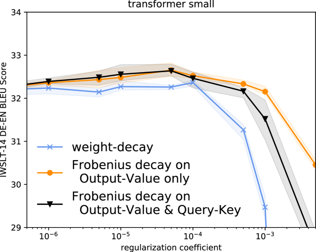
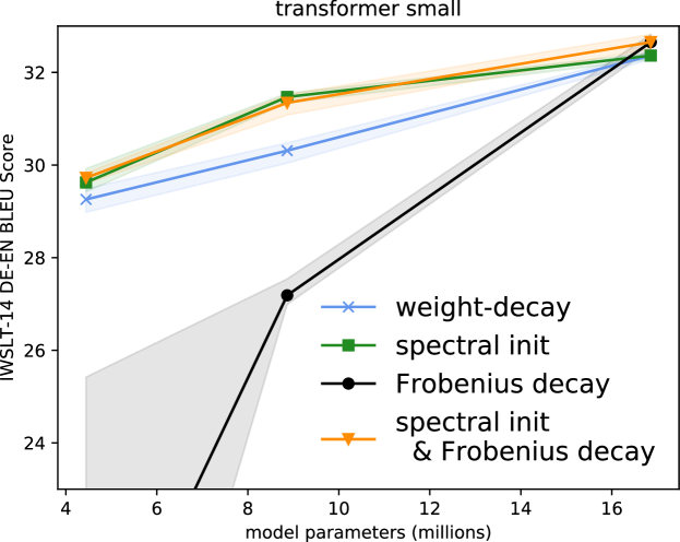
Figure 4: Transformer performance on IWSLT-14 as a function of regularization (top) and compression (bottom).

Table 4: Comparison of BERT unsupervised pretraining using LAMB (You et al., 2020) and our Frobenius decay scheme FLAMBé. Evaluation is conducted by fine-tuning the final model on the SQuAD question-answering task (Rajpurkar et al., 2016). Guided by IWSLT results, FLAMBé is applied only to the Output-Value form in MHA; regular weight-decay is used on all other parameters. Spectral initialization of MHA is used for FLAMBé as well, but we find the effect minimal. Regularization coefficients for both methods were obtained by tuning on the uncompressed model, targeting the unsupervised loss.

		compression	param.
		rate	count	SQuAD
model	optimizer	(MHA-only)	(M)	F1	EM
BERT base	LAMB	1.0	110	88.55	81.06
	LAMB (SI & FD)	1.0	110	88.16	80.86
	FLAMBé (SI & FD)	1.0	110	88.88	81.54
	LAMB	0.5	95.7	87.35	79.83
	FLAMBé (SI & FD)	0.5	95.7	87.69	80.42
BERT	LAMB	1.0	340	91.41	84.99
large	FLAMBé (SI & FD)	0.5	295.8	90.55	83.82

7 Conclusion

In this paper we studied the design of training algorithms for deep nets containing factorized layers, demonstrating that two simple specializations of standard initialization and regularization schemes from the unfactorized case lead to strong improvements for model compression, knowledge distillation, and MHA-based architectures. While we largely focused on the case where the unfactorized model uses Gaussian initialization and $\ell_{2}$-regularization, we believe our work provides guidance for the many cases where other schemes are used to enforce alternative priors or improve optimization. For example, SI as defined can be applied to any random initialization, while our FD results suggest that regularizers such as penalty terms and DropConnect (Wan et al., 2013) should be applied on the product matrix rather than directly on individual factors. The success of SI and FD for both low-rank and tensor decomposition also suggests that these schemes may be useful for other types of factorized neural layers, such as ACDC (Moczulski et al., 2015) or K-matrices (Dao et al., 2020).

Appendix A Generalization Error of Factorized Layers

In this section we briefly discuss how to apply the generalization bounds in Neyshabur et al. (2018) to factorized models.

Definition A.1.

For any $\gamma>0$ and distribution ${\mathcal{D}}$ over classification data ${\mathcal{X}}\times{\mathcal{Y}}$ the $\gamma$-margin-loss of a model $f_{\theta}:{\mathcal{X}}\mapsto{\mathcal{Y}}$ is defined as $\ell_{\mathcal{D}}^{\gamma}(f_{\theta})=\mathbb{P}_{({\bm{x}},y)\sim{\mathcal{D}}}\left(f_{\theta}({\bm{x}})[y]\leq\gamma+\max_{y^{\prime}\neq y}f_{\theta}({\bm{x}})[y^{\prime}]\right)$.

Note that $\ell_{\mathcal{D}}^{0}$ is the expected classification loss over the distribution and $\ell_{\operatorname{Uniform}({\mathcal{S}})}^{\gamma}$ is the empirical $\gamma$-margin-loss. We have the following corollaries:

Corollary A.1.

Let $f_{\theta}$ be a neural network with $L-1$ factorized fully-connected ReLU layers $g_{i}({\bm{U}}_{i}{\bm{V}}_{i}^{T},{\bm{x}}_{i-1})=\max\left\{{\bm{U}}_{i}{\bm{V}}_{i}^{T}{\bm{x}}_{i-1},{\bm{0}}_{m}\right\}$ of hidden dimension $m$ and one factorized classification layer $g_{L}({\bm{U}}_{L}{\bm{V}}_{L}^{T},{\bm{x}}_{L-1})={\bm{U}}_{L}{\bm{V}}_{L}^{T}{\bm{x}}_{L-1}$. Let ${\mathcal{D}}$ be a distribution over $B$-bounded classification data ${\mathcal{X}}\times{\mathcal{Y}}$ and suppose we have a finite set ${\mathcal{S}}$ of i.i.d. samples from it. If $\operatorname{rank}({\bm{U}}_{i}{\bm{V}}_{i}^{T})\leq r$ and $\|{\bm{U}}_{i}{\bm{V}}_{i}^{T}\|_{2}\}\leq\sigma$ for all $i$ then for any $\delta>0$ we have w.p. $1-\delta$ that

$$\ell_{\mathcal{D}}^{0}(f_{\theta})\leq\ell_{\operatorname{Uniform}({\mathcal{S}})}^{\gamma}+{\mathcal{O}}\left(\sqrt{\frac{B^{2}L^{3}m\sigma^{2L}r\log(Lm)\prod_{i=1}^{L}\|{\bm{U}}_{i}{\bm{V}}_{i}^{T}\|_{2}^{2}+\log\frac{L|{\mathcal{S}}|}{\delta}}{\gamma^{2}|{\mathcal{S}}|}}\right)$$ (4)

Proof.

Apply the inequality $\|{\bm{W}}_{i}\|_{F}^{2}/\|{\bm{W}}_{i}\|_{2}^{2}\leq\operatorname{rank}({\bm{W}}_{i})$ to Neyshabur et al. (2018, Theorem 1) and substitute ${\bm{W}}_{i}={\bm{U}}_{i}{\bm{V}}_{i}^{T}$. ∎

Corollary A.2.

Let $f_{\theta}$ be a neural network with $L-1$ factorized fully-connected ReLU layers $g_{i}({\bm{U}}_{i}(\prod_{j=1}^{d}{\bm{M}}_{ij}){\bm{V}}_{i}^{T},{\bm{x}}_{i-1})=\max\left\{{\bm{U}}_{i}(\prod_{j=1}^{d}{\bm{M}}_{ij}){\bm{V}}_{i}^{T}{\bm{x}}_{i-1},{\bm{0}}_{m}\right\}$ of hidden dimension $m$ and one factorized classification layer $g_{L}({\bm{U}}_{L}(\prod_{j=1}^{d}{\bm{M}}_{Lj}){\bm{V}}_{L}^{T},{\bm{x}}_{L-1})={\bm{U}}_{L}(\prod_{j=1}^{d}{\bm{M}}_{Lj}){\bm{V}}_{L}^{T}{\bm{x}}_{L-1}$. Let ${\mathcal{D}}$ be a distribution over $B$-bounded classification data ${\mathcal{X}}\times{\mathcal{Y}}$ from which we have a finite set ${\mathcal{S}}$ of i.i.d. samples. If $\|{\bm{U}}_{i}\prod_{j=1}^{d}{\bm{M}}_{ij}{\bm{V}}_{i}^{T}\|_{2}\}\leq\sigma$ for all $i$ then for any $\delta>0$ we have w.p. $1-\delta$ that

$$\ell_{\mathcal{D}}^{0}(f_{\theta})\leq\ell_{\operatorname{Uniform}({\mathcal{S}})}^{\gamma}+{\mathcal{O}}\left(\sqrt{\frac{B^{2}L^{2}m\sigma^{2L-2}\log(Lm)\sum_{i=1}^{L}\|{\bm{U}}_{i}(\prod_{j=1}^{d}{\bm{M}}_{ij}){\bm{V}}_{i}^{T}\|_{F}^{2}+\log\frac{L|{\mathcal{S}}|}{\delta}}{\gamma^{2}|{\mathcal{S}}|}}\right)$$ (5)

Proof.

Apply the equality $\left(\prod_{i=1}^{L}\|{\bm{W}}_{i}\|_{2}^{2}\right)\sum_{i=1}^{L}\frac{\|{\bm{W}}_{i}\|_{F}^{2}}{\|{\bm{W}}_{i}\|_{2}^{2}}=\sum_{i=1}^{L}\|{\bm{W}}_{i}\|_{F}^{2}\prod_{j\neq i}\|{\bm{W}}_{j}\|_{2}^{2}$ to Neyshabur et al. (2018, Theorem 1) and substitute ${\bm{W}}_{i}={\bm{U}}_{i}(\prod_{j=1}^{d}{\bm{M}}_{ij}){\bm{V}}_{i}^{T}$. ∎

Appendix B Proof of Claim 3.1

Proof.

Let $\rho_{t}=\|{\bm{W}}_{t}\|_{F}$ be the Frobenius norm of the composed matrix at time $t$. Applying the update rules for ${\bm{U}}_{t}$ and ${\bm{V}}_{t}$ and using the fact that $\rho_{t}\nabla_{{\bm{W}}_{t}}=\nabla_{\hat{\bm{W}}_{t}}$ yields

$$\begin{split}{\bm{W}}_{t+1}=({\bm{U}}_{t}-\eta\nabla_{{\bm{U}}_{t}})({\bm{V}}_{t}^{T}-\eta\nabla_{{\bm{V}}_{t}^{T}})&=({\bm{U}}_{t}-\eta\nabla_{{\bm{W}}_{t}}{\bm{V}}_{t})({\bm{V}}_{t}^{T}-\eta{\bm{U}}_{t}^{T}\nabla_{{\bm{W}}_{t}^{T}})\\ &={\bm{W}}_{t}-\frac{\eta}{\rho_{t}}\hat{\nabla}_{t}+\eta^{2}\nabla_{{\bm{W}}_{t}}{\bm{W}}_{t}^{T}\nabla_{{\bm{W}}_{t}}\end{split}$$ (6)

Taking the squared norm of both sides yields $\rho_{t+1}^{2}=\rho_{t}^{2}-2\eta\operatorname{Tr}(\hat{\bm{W}}_{t}^{T}\hat{\nabla}_{t})+{\mathcal{O}}(\eta^{2})$; we can then take the square root of both sides and use a Tayor expansion to obtain

$$\rho_{t+1}=\rho_{t}\sqrt{1-\frac{2\eta}{\rho_{t}^{2}}\operatorname{Tr}(\hat{\bm{W}}_{t}^{T}\hat{\nabla}_{t})+{\mathcal{O}}(\eta^{2})}=\rho_{t}-\frac{\eta}{\rho_{t}}\operatorname{Tr}(\hat{\bm{W}}_{t}^{T}\hat{\nabla}_{t})+{\mathcal{O}}(\eta^{2})$$ (7)

Then, starting from Equation 6 divided by $\rho_{t+1}$, substituting Equation 7, and applying a Taylor expansion yields

$$\begin{split}\hat{\bm{W}}_{t+1}&=\frac{\rho_{t}}{\rho_{t+1}}\hat{\bm{W}}_{t}-\frac{\eta}{\rho_{t}\rho_{t+1}}\hat{\nabla}_{t}+{\mathcal{O}}(\eta^{2})\\ &=\frac{1}{1-\frac{\eta}{\rho_{t}^{2}}\operatorname{Tr}(\hat{\bm{W}}_{t}^{T}\hat{\nabla}_{t})}\hat{\bm{W}}_{t}-\frac{\eta}{\rho_{t}^{2}-\eta\operatorname{Tr}(\hat{\bm{W}}_{t}^{T}\hat{\nabla}_{t})}\hat{\nabla}_{t}+{\mathcal{O}}(\eta^{2})\\ &=\left(1+\frac{\eta}{\rho_{t}^{2}}\operatorname{Tr}(\hat{\bm{W}}_{t}^{T}\hat{\nabla}_{t})\right)\hat{\bm{W}}_{t}-\frac{\eta}{\rho_{t}^{2}}\hat{\nabla}_{t}+{\mathcal{O}}(\eta^{2})\\ &=\hat{\bm{W}}_{t}-\frac{\eta}{\rho_{t}^{2}}(\hat{\nabla}_{t}-(\hat{\bm{w}}_{t}^{T}\operatorname{vec}(\hat{\nabla}_{t}))\hat{\bm{W}}_{t})+{\mathcal{O}}(\eta^{2})\end{split}$$ (8)

Vectorizing and observing that $(\hat{\bm{w}}_{t}^{T}\operatorname{vec}(\hat{\nabla}_{t}))\hat{\bm{w}}_{t}=\hat{\bm{w}}_{t}\hat{\bm{w}}_{t}^{T}\operatorname{vec}(\hat{\nabla}_{t})$ yields the result. ∎

Appendix C Experimental Details for Training Convolutional Networks

For experiments with regular ResNets on CIFAR we used code provided here: https://github.com/akamaster/pytorch_resnet_cifar10. All hyperparameter settings are the same, except initialization and regularization as appropriate, with the exception that we use a warmup epoch with a 10 times smaller learning rate for ResNet56 for stability (this is already done by default for ResNet110).

For comparisons with sparse model training of ResNet32${}^{\textrm{x2}}$ and VGG19${}^{\textrm{NFC}}$ we use code by Wang et al. (2019, https://github.com/alecwangcq/EigenDamage-Pytorch), which is closely related to that of the lottery-ticket-guessing paper by Wang et al. (2020). All hyperparameter settings are the same, except (1) initialization and regularization as appropriate and (2) for Tiny-ImageNet we only train for 200 epochs instead of 300.

For comparisons with tensor decomposition training of WideResNet we use code by Gray et al. (2019, https://github.com/BayesWatch/deficient-efficient). All hyperparameter settings are the same, except initialization and regularization as appropriate.

Table 5: Pruning, sparse training, and low-rank training for VGG-19${}^{\textrm{NFC}}$, i.e. the model of Simonyan & Zisserman (2015) with no fully-connected layers, as in Wang et al. (2020).

CIFAR-10	uncompressed	0.1	0.05	0.02
baseline∗	94.23
baseline†	93.70
baseline (reproduced)	93.75$\pm$0.48
OBD∗ LeCun et al. (1990)		93.74	93.58	93.49
MLPrune∗ (Zeng & Urtasun, 2019)		93.83	93.69	93.49
LT∗, original initialization		93.51	92.92	92.34
LT∗, reset to epoch 5		93.82	93.61	93.09
LR Rewinding† (Renda et al., 2020)		94.14$\pm$0.17	93.99$\pm$0.15	10.00$\pm$0.00
Hybrid Tickets† (Su et al., 2020)		94.00$\pm$0.12	93.83$\pm$0.10	93.52$\pm$0.28
DSR∗ (Mostafa & Wang, 2019)		93.75	93.86	93.13
SET∗ (Mocanu et al., 2018)		92.46	91.73	89.18
Deep-R∗ (Bellec et al., 2018)		90.81	89.59	86.77
SNIP∗ (Lee et al., 2018)		93.63$\pm$0.06	93.43$\pm$0.20	92.05$\pm$0.28
GraSP∗ (Wang et al., 2020)		92.59$\pm$0.10	91.01$\pm$0.21	87.51$\pm$0.31
Random Tickets† (Su et al., 2020)		93.77$\pm$0.10	93.42$\pm$0.22	92.45$\pm$0.22
Low-Rank		90.71$\pm$0.42	88.08$\pm$0.14	80.81$\pm$0.85
Low-Rank (SI)		90.99$\pm$0.34	88.61$\pm$0.95	82.53$\pm$0.14
Low-Rank (FD)		91.57$\pm$0.26	88.16$\pm$0.50	82.81$\pm$0.37
Low-Rank (SI & FD)		91.58$\pm$0.27	88.98$\pm$0.18	83.27$\pm$0.56
CIFAR-100	uncompressed	0.1	0.05	0.02
baseline∗	74.16
baseline†	72.60
baseline (reproduced)	73.42$\pm$0.17
OBD∗ LeCun et al. (1990)		73.83	71.98	67.79
MLPrune∗ (Zeng & Urtasun, 2019)		73.79	73.07	71.69
LT∗, original initialization		72.78	71.44	68.95
LT∗, reset to epoch 5		74.06	72.87	70.55
LR Rewinding† (Renda et al., 2020)		73.73$\pm$0.18	72.39$\pm$0.40	1.00$\pm$0.00
Hybrid Tickets† (Su et al., 2020)		73.53$\pm$0.20	73.10$\pm$0.11	71.61$\pm$0.46
DSR∗ (Mostafa & Wang, 2019)		72.31	71.98	70.70
SET∗ (Mocanu et al., 2018)		72.36	69.81	65.94
Deep-R∗ (Bellec et al., 2018)		66.83	63.46	59.58
SNIP∗ (Lee et al., 2018)		72.84$\pm$0.22	71.83$\pm$0.23	58.46$\pm$1.10
GraSP∗ (Wang et al., 2020)		71.95$\pm$0.18	71.23$\pm$0.12	68.90$\pm$0.47
Random Tickets† (Su et al., 2020)		72.55$\pm$0.14	71.37$\pm$0.09	68.98$\pm$0.34
Low-Rank		62.32$\pm$0.26	54.97$\pm$5.28	42.80$\pm$3.14
Low-Rank (SI)		63.77$\pm$0.93	58.51$\pm$1.90	45.02$\pm$3.24
Low-Rank (FD)		64.07$\pm$1.58	59.34$\pm$2.97	45.73$\pm$2.62
Low-Rank (SI & FD)		65.61$\pm$1.48	60.1$\pm$1.29	46.43$\pm$1.26
Tiny-ImageNet	uncompressed	0.1	0.05	0.02
baseline∗	61.38
baseline†	61.57
baseline (reproduced)	62.19$\pm$0.74
OBD∗ LeCun et al. (1990)		61.21	60.49	54.98
MLPrune∗ (Zeng & Urtasun, 2019)		60.23	59.23	55.55
LT∗, original initialization		60.32	59.48	55.12
LT∗, reset to epoch 5		61.19	60.57	56.18
DSR∗ (Mostafa & Wang, 2019)		62.43	59.81	58.36
SET∗ (Mocanu et al., 2018)		62.49	59.42	56.22
Deep-R∗ (Bellec et al., 2018)		55.64	52.93	49.32
SNIP∗ (Lee et al., 2018)		61.02$\pm$0.41	59.27$\pm$0.39	48.95$\pm$1.73
GraSP∗ (Wang et al., 2020)		60.76$\pm$0.23	59.50$\pm$0.33	57.28$\pm$0.34
Random Tickets† (Su et al., 2020)		60.94$\pm$0.38	59.48$\pm$0.43	55.87$\pm$0.16
Low-Rank		48.50$\pm$3.43	46.98$\pm$1.68	36.57$\pm$1.03
Low-Rank (SI)		49.87$\pm$1.39	46.73$\pm$2.83	37.25$\pm$0.19
Low-Rank (FD)		53.93$\pm$0.66	47.95$\pm$1.13	35.63$\pm$0.71
Low-Rank (SI & FD)		53.53$\pm$0.45	47.60$\pm$0.51	35.68$\pm$0.64

• Obtained from Wang et al. (2020).

• Obtained from Su et al. (2020).

Table 6: Pruning, sparse training, and low-rank training for ResNet-32${}^{\textrm{x2}}$, i.e. the model of He et al. (2016) with twice the number of filters, as in Wang et al. (2020).

CIFAR-10	uncompressed	0.1	0.05	0.02
baseline∗	94.80
baseline†	94.62
baseline (reproduced)	94.49$\pm$0.29
OBD∗ LeCun et al. (1990)		94.17	93.29	90.31
MLPrune∗ (Zeng & Urtasun, 2019)		94.21	93.02	89.65
LT∗, original initialization		92.31	91.06	88.78
LT∗, reset to epoch 5		93.97	92.46	89.18
LR Rewinding† (Renda et al., 2020)		94.14$\pm$0.10	93.02$\pm$0.28	90.83$\pm$0.22
Hybrid Tickets† (Su et al., 2020)		93.98$\pm$0.15	92.96$\pm$0.13	90.85$\pm$0.06
DSR∗ (Mostafa & Wang, 2019)		92.97	91.61	88.46
SET∗ (Mocanu et al., 2018)		92.30	90.76	88.29
Deep-R∗ (Bellec et al., 2018)		91.62	89.84	86.45
SNIP∗ (Lee et al., 2018)		92.59$\pm$0.10	91.01$\pm$0.21	87.51$\pm$0.31
GraSP∗ (Wang et al., 2020)		92.38$\pm$0.21	91.39$\pm$0.25	88.81$\pm$0.14
Random Tickets† (Su et al., 2020)		92.97$\pm$0.05	91.60$\pm$0.26	89.10$\pm$0.33
Low-Rank		93.59$\pm$0.12	92.45$\pm$0.69	87.95$\pm$0.91
Low-Rank (SI)		92.52$\pm$0.66	91.72$\pm$0.63	87.36$\pm$0.65
Low-Rank (FD)		92.92$\pm$0.29	89.44$\pm$0.25	83.05$\pm$1.02
Low-Rank (SI & FD)		94.34$\pm$0.34	92.90$\pm$0.43	87.97$\pm$0.86
CIFAR-100	uncompressed	0.1	0.05	0.02
baseline∗	74.64
baseline†	74.57
baseline (reproduced)	75.41$\pm$1.26
OBD∗ LeCun et al. (1990)		71.96	68.73	60.65
MLPrune∗ (Zeng & Urtasun, 2019)		72.34	67.58	59.02
LT∗, original initialization		68.99	65.02	57.37
LT∗, reset to epoch 5		71.43	67.28	58.95
LR Rewinding† (Renda et al., 2020)		72.41$\pm$0.49	67.22$\pm$3.42	59.22$\pm$1.15
Hybrid Tickets† (Su et al., 2020)		71.47$\pm$0.26	69.28$\pm$0.40	63.44$\pm$0.34
DSR∗ (Mostafa & Wang, 2019)		69.63	68.20	61.24
SET∗ (Mocanu et al., 2018)		69.66	67.41	62.25
Deep-R∗ (Bellec et al., 2018)		66.78	63.90	58.47
SNIP∗ (Lee et al., 2018)		68.89$\pm$0.45	65.22$\pm$0.69	54.81$\pm$1.43
GraSP∗ (Wang et al., 2020)		69.24$\pm$0.24	66.50$\pm$0.11	58.43$\pm$0.43
Random Tickets† (Su et al., 2020)		69.70$\pm$0.48	66.82$\pm$0.12	60.11$\pm$0.16
Low-Rank		72.71$\pm$0.43	67.86$\pm$0.91	61.08$\pm$0.76
Low-Rank (SI)		71.71$\pm$1.46	67.41$\pm$1.12	60.79$\pm$0.26
Low-Rank (FD)		71.85$\pm$0.39	66.89$\pm$0.73	55.31$\pm$0.61
Low-Rank (SI & FD)		74.41$\pm$0.67	70.22$\pm$0.64	61.40$\pm$0.96
Tiny-ImageNet	uncompressed	0.15	0.1	0.1
baseline∗	62.89
baseline†	62.92
baseline (reproduced)	63.02$\pm$0.94
OBD∗ LeCun et al. (1990)		58.55	56.80	51.00
MLPrune∗ (Zeng & Urtasun, 2019)		58.86	57.62	51.70
LT∗, original initialization		56.52	54.27	49.47
LT∗, reset to epoch 5		60.31	57.77	51.21
DSR∗ (Mostafa & Wang, 2019)		57.08	57.19	56.08
SET∗ (Mocanu et al., 2018)		57.02	56.92	56.18
Deep-R∗ (Bellec et al., 2018)		53.29	52.62	52.00
SNIP∗ (Lee et al., 2018)		56.33$\pm$0.24	55.43$\pm$0.14	49.57$\pm$0.44
GraSP∗ (Wang et al., 2020)		57.25$\pm$0.11	55.53$\pm$0.11	51.34$\pm$0.29
Random Tickets† (Su et al., 2020)		N/A	55.26$\pm$0.22	51.41$\pm$0.38
Low-Rank		60.82$\pm$0.72	58.72$\pm$0.53	55.39$\pm$1.02
Low-Rank (SI)		59.53$\pm$1.41	57.60$\pm$0.88	55.00$\pm$0.90
Low-Rank (FD)		59.45$\pm$0.82	57.24$\pm$0.61	54.15$\pm$1.22
Low-Rank (SI & FD)		62.24$\pm$0.39	60.25$\pm$1.02	55.97$\pm$0.48

• Obtained from Wang et al. (2020).

• Obtained from Su et al. (2020).

Table 7: Comparison of low-rank and tensor-decomposition training (mean of 3 trials) of WideResNet28-10 on CIFAR-10. The best error for each compression-decomposition setting is bolded; in addition, the best error at each compression level is underlined.

			initialization
compression	decomposition	decay ($\lambda=0.005$)	default	spectral
none ($\approx$36.5 param.)			3.21$\pm$0.22
0.01667 ($\approx$0.61M param.)		regular	7.62$\pm$0.08	7.72$\pm$0.11
	Low-Rank	CRS∗	8.63$\pm$0.87	8.83$\pm$0.17
		Frobenius	7.23$\pm$0.32	7.26$\pm$0.45
		regular	8.55$\pm$4.22	7.72$\pm$0.46
	Tensor-Train	CRS∗	7.01$\pm$0.35	6.52$\pm$0.17
		Frobenius	7.26$\pm$0.73	6.22$\pm$0.50
		regular	10.67$\pm$7.68	9.91$\pm$6.71
	Tucker	CRS∗	8.28$\pm$0.05	6.79$\pm$0.34
		Frobenius	8.65$\pm$0.27	7.07$\pm$0.28
0.06667 ($\approx$2.4M param.)		regular	5.31$\pm$0.06	5.49$\pm$0.42
	Low-Rank	CRS∗	5.86$\pm$0.22	5.53$\pm$0.72
		Frobenius	3.89$\pm$0.17	3.86$\pm$0.22
		regular	7.33$\pm$0.27	6.49$\pm$0.30
	Tensor-Train	CRS∗	5.20$\pm$0.37	4.79$\pm$0.15
		Frobenius	5.02$\pm$0.15	5.10$\pm$0.35
		regular	5.64$\pm$0.19	5.61$\pm$0.46
	Tucker	CRS∗	5.30$\pm$0.35	5.15$\pm$0.23
		Frobenius	5.30$\pm$0.12	5.24$\pm$0.21

• Regular weight-decay with coefficient scaled by the compression rate (Gray et al., 2019).

Table 8: Overcomplete ResNet performance (mean of 3 trials). The best accuracy at each depth is bolded; cases where we match the next deeper network with around the same training memory are underlined. Note that training times are reported for roughly similar machine types; all ResNet56 and ResNet110 times are reported on identical machine types.

CIFAR-10			factorization type
depth	decay type/metric	unfactorized	full	deep	wide
	WD test accuracy	$92.66\pm 0.34$	$92.11\pm 0.36$	$91.37\pm 0.09$	$92.26\pm 0.35$
	training time (H)	$1.51\pm 0.17$	$1.86\pm 0.23$	$2.10\pm 0.14$	$2.20\pm 0.22$
32	FD test accuracy		$\underline{93.32\pm 0.07}$	$93.11\pm 0.13$	$\mathbf{93.36\pm 0.11}$
	training time (H)		$1.60\pm 0.22$	$2.40\pm 0.16$	$1.97\pm 0.23$
	training param. (M)	0.46	0.95	1.43	2.84
	WD test accuracy	$93.15\pm 0.56$	$92.95\pm 0.24$	$92.52\pm 0.13$	$93.08\pm 0.23$
	training time (H)	$1.39\pm 0.04$	$2.12\pm 0.00$	$2.45\pm 0.12$	$3.51\pm 0.09$
56	FD test accuracy		$\underline{\mathbf{94.13\pm 0.16}}$	$93.89\pm 0.13$	$93.83\pm 0.10$
	training time (H)		$2.22\pm 0.07$	$2.89\pm 0.05$	$3.65\pm 0.14$
	training param. (M)	0.85	1.72	2.59	5.16
	WD test accuracy	$93.61\pm 0.28$	$93.73\pm 0.16$	$93.25\pm 0.07$	$93.53\pm 0.07$
	training time (H)	$3.51\pm 0.06$	$3.86\pm 0.13$	$4.92\pm 0.15$	$6.37\pm 0.21$
110	FD test accuracy		$94.28\pm 0.05$	$\mathbf{94.42\pm 0.09}$	$94.13\pm 0.05$
	training time (H)		$4.18\pm 0.04$	$5.77\pm 0.22$	$6.55\pm 0.18$
	training param. (M)	1.73	3.47	5.21	10.39
CIFAR-100			factorization type
depth	metric	unfactorized	full	deep	wide
	WD test accuracy	$68.17\pm 0.48$	$68.84\pm 0.27$	$67.84\pm 0.50$	$69.23\pm 0.32$
	training time (H)	$1.60\pm 0.21$	$1.80\pm 0.23$	$1.61\pm 0.04$	$2.48\pm 0.19$
32	FD test accuracy		$\underline{70.32\pm 0.41}$	$70.25\pm 0.46$	$\mathbf{70.53\pm 0.07}$
	training time (H)		$1.61\pm 0.10$	$2.13\pm 0.20$	$2.61\pm 0.18$
	training param. (M)	0.47	0.95	1.44	2.84
	WD test accuracy	$70.25\pm 0.30$	$70.6\pm 0.53$	$69.62\pm 0.35$	$70.69\pm 0.21$
	training time (H)	$1.39\pm 0.04$	$2.09\pm 0.04$	$2.59\pm 0.04$	$3.48\pm 0.27$
56	FD test accuracy		$\underline{72.79\pm 0.37}$	$72.28\pm 0.26$	$\mathbf{73.01\pm 0.39}$
	training time (H)		$2.30\pm 0.05$	$2.96\pm 0.17$	$3.33\pm 0.19$
	training param. (M)	0.86	1.73	2.60	5.17
	WD test accuracy	$72.11\pm 0.37$	$72.33\pm 0.57$	$71.28\pm 0.62$	$71.70\pm 0.55$
	training time (H)	$3.87\pm 0.08$	$3.78\pm 0.04$	$4.95\pm 0.23$	$6.12\pm 0.25$
110	FD test accuracy		$73.98\pm 0.22$	$\mathbf{74.17\pm 0.23}$	$73.69\pm 0.72$
	training time (H)		$4.46\pm 0.07$	$5.66\pm 0.18$	$6.81\pm 0.18$
	training param. (M)	1.73	3.48	5.22	10.40

Appendix D Experimental Details for Training Transformer Models

For experiments with Transformer models on machine translation we used code provided here: https://github.com/StillKeepTry/Transformer-PyTorch. All hyperparameter settings are the same, except initialization and regularization as appropriate.

For comparisons with LAMB optimization of BERT, we use an implementation provided by NVIDIA: https://github.com/NVIDIA/DeepLearningExamples/tree/master/PyTorch/LanguageModeling/BERT. All hyperparameter settings are the same, except initialization and regularization as appropriate. For fine-tuning on SQuAD we apply the same optimization routine to all pre-trained models.

Appendix E Past Work on Knowledge Distillation

We first briefly summarize past work on overcomplete KD. While the use of factorized neural layers for improving training has theoretical roots (Arora et al., 2018; Du & Hu, 2019), we are aware of two other works focusing on experimental practicality: ExpandNets (Guo et al., 2020) and DO-Conv (Cao et al., 2020). As the former focuses on small student networks, numerically we compare directly to the latter, showing much better improvement due to distillation for both ResNet56 and ResNet110 on both CIFAR-10 and CIFAR-100 in Table 3. Note that we are also aware of one paper proposing a related method that also trains an over-parameterized model without increasing expressivity that can then be collapsed into a smaller “original” model (Ding et al., 2019); their approach, called ACNet, passes the input to each layer through differently-shaped kernels that can be composed additively. Note that it is unclear how to express this method as a factorization and it may not be easy to generalize to non-convolutional networks, so we do not view it as an overcomplete KD approach.

We now conduct a brief comparison with both these works and more standard approaches to KD. Direct comparison with past work is made difficult by the wide variety of training routines, teacher models, student models, and evaluation procedures employed by the community. Comparing our specific approach is made even more difficult by the fact that we have no teacher network, or at least not one that is a standard model used in computer vision. Nevertheless, in Table 9 we collect an array of existing results that can be plausibly compared to our own overcomplete distillation of ResNets. Even here, note that absolute numbers vary significantly, so we focus on changes in accuracy. As can be seen from the results, our overcomplete approach yields the largest improvements for ResNet56 and ResNet110 on both CIFAR-10 and CIFAR-100. For ResNet32, the Snapshot Distillation method of Xu & Liu (2019) outperforms our own, although it does not do so for ResNet110 and is not evaluated for ResNet56. On CIFAR-10 the additive ACNet approach also has a larger performance improvement for ResNet32. Nevertheless, our method is still fairly close in these cases, so the results in Table 9 together with the simplicity and short (single-stage) distillation routine of our overcomplete approach suggest that it should be a standard baseline for KD.

Table 9: Comparison of our knowledge distillation approach with past work in which the same student network attains roughly similar performance.

CIFAR-10			reported	reported	change
baseline			baseline	distilled	in
depth	method (source)	teacher	accuracy	accuracy	accuracy
32	SD (Xu & Liu, 2019)	self	92.78	93.68	+0.90
	ACNet (Ding et al., 2019)	additive	94.31	95.09	+0.78
	wide factorization w. FD (ours)	overcomplete	92.66	93.36	+0.70
56	KD-fn (Xu et al., 2020)	ResNet110	93.63	94.14	+0.51
	DO-Conv (Cao et al., 2020)	overcomplete	93.26	93.38	+0.12
	full factorization w. FD (ours)	overcomplete	93.15	94.13	+0.98
110	SD (Xu & Liu, 2019)	self	94.00	94.43	+0.43
	DO-Conv (Cao et al., 2020)	overcomplete	93.72	93.93	+0.21
	deep factorization w. FD (ours)	overcomplete	93.61	94.42	+0.81
CIFAR-100			reported	reported	change
baseline			baseline	distilled	in
depth	method (source)	teacher	accuracy	accuracy	accuracy
32	CRD (Tian et al., 2020)	ResNet110	71.14	73.48	+2.34
	SD (Xu & Liu, 2019)	self	68.99	71.78	+2.79
	Snapshot (Yang et al., 2019)	self	68.39	69.84	+1.45
	ACNet (Ding et al., 2019)	additive	73.58	74.04	+0.46
	wide factorization w. FD (ours)	overcomplete	68.17	70.53	+2.36
56	FT (Kim et al., 2018)	ResNet110	71.96	74.38	+2.42
	Snapshot (Yang et al., 2019)	self	70.06	70.78	+0.72
	DO-Conv (Cao et al., 2020)	overcomplete	70.15	70.78	+0.63
	wide factorization w. FD (ours)	overcomplete	70.25	73.01	+2.76
110	SD (Xu & Liu, 2019)	self	73.21	74.96	+1.75
	Snapshot (Yang et al., 2019)	self	71.47	72.48	+1.01
	DO-Conv (Cao et al., 2020)	overcomplete	72.00	72.22	+0.22
	deep factorization w. FD (ours)	overcomplete	72.11	74.17	+2.06

References

- Arora et al. (2018) Sanjeev Arora, Nadav Cohen, and Elad Hazan. On the optimization of deep networks: Implicit acceleration by overparameterization. In Proceedings of the 35th International Conference on Machine Learning, 2018.
- Ba et al. (2016) Jimmy Lei Ba, Jamie Ryan Kiros, and Geoffrey E. Hinton. Layer normalization. arXiv, 2016.
- Bai & Yin (1993) Z. D. Bai and Y. Q. Yin. Limit of the smallest eigenvalue of a large dimensional sample covariance matrix. The Annals of Probability, 21(3):1275–1294, 1993.
- Bellec et al. (2018) Guillaume Bellec, David Kappel, Wolfgang Maass, and Robert Legenstein. Deep rewiring: Training very sparse deep networks. In Proceedings of the 6th International Conference on Learning Representations, 2018.
- Bernacchia et al. (2018) Alberto Bernacchia, Máté Lengyel, and Guillaume Hennequin. Exact natural gradient in deep linear networks and application to the nonlinear case. In Advances in Neural Information Processing Systems, 2018.
- Blalock et al. (2020) Davis Blalock, Jose Javier Gonzalez Ortiz, Jonathan Frankle, and John Guttag. What is the state of neural network pruning? In Proceedings of Machine Learning and Systems, 2020.
- Cai et al. (2019) Changxiao Cai, Gen Li, H. Vincent Poor, and Yuxin Chen. Nonconvex low-rank tensor completion from noisy data. In Advances in Neural Information Processing Systems, 2019.
- Cao et al. (2020) Jinming Cao, Yangyan Li, Mingchao Sun, Ying Chen, Dani Lischinski, Daniel Cohen-Or, Baoquan Chen, and Changhe Tu. DO-Conv: Depthwise over-parameterized convolutional layer. arXiv, 2020.
- Cettolo et al. (2014) Mauro Cettolo, Jan Niehues, Sebastian Stüker, Luisa Bentivogli, and Marcello Federico. Report on the 11th IWSLT evaluation campaign. In Proceedings of the International Workshop on Spoken Language Translation, 2014.
- Chi et al. (2019) Yuejie Chi, Yue M. Lu, and Yuxin Chen. Nonconvex optimization meets low-rank matrix factorization. IEEE Transactions on Signal Processing, 67:5239–5269, 2019.
- Dao et al. (2020) Tri Dao, Nimit Sohoni, Albert Gu, Matthew Eichhorn, Amit Blonder, Megan Leszczynski, Atri Rudra, and Christopher Ré. Kaleidoscope: An efficient, learnable representation for all structured linear maps. In Proceedings of the 8th International Conference on Learning Representations, 2020.
- Deng et al. (2009) Jia Deng, Wei Dong, Richard Socher, Li-Jia Li, Kai Li, and Li Fei-Fei. ImageNet: A large-scale hierarchical image database. In Proceedings of the IEEE Conference on Computer Vision and Pattern Recognition, 2009.
- Denil et al. (2013) Misha Denil, Babak Shakibi, Laurent Dinh, Marc’Aurelio Ranzato, and Nando de Freitas. Predicting parameters in deep learning. In Advances in Neural Information Processing Systems, 2013.
- Devlin et al. (2019) Jacob Devlin, Ming-Wei Chang, Kenton Lee, and Kristina Toutanova. BERT: Pre-training of deep bidirectional transformers for language understanding. In Proceedings of the North American Chapter of the Association for Computational Linguistics: Human Language Technologies, 2019.
- Ding et al. (2019) Xiaohan Ding, Yuchen Guo, Guiguang Ding, and Jungong Han. ACNet: Strengthening the kernel skeletons for powerful CNN via asymmetric convolution blocks. In Proceedings of the IEEE International Conference on Computer Vision, 2019.
- Du & Hu (2019) Simon S. Du and Wei Hu. Width provably matters in optimization for deep linear neural networks. In Proceedings of the 36th International Conference on Machine Learning, 2019.
- Frankle & Carbin (2019) Jonathan Frankle and Michael Carbin. The lottery ticket hypothesis: Finding sparse, trainable neural. In Proceedings of the 7th International Conference on Learning Representations, 2019.
- Gehring et al. (2017) Jonas Gehring, Michael Auli, David Grangier, Denis Yarats, and Yann N. Dauphin. Convolutional sequence to sequence learning. In Proceedings of the 35th International Conference on Machine Learning, 2017.
- Gray et al. (2019) Gavin Gray, Elliot J. Crowley, and Amos Storkey. Separable layers enable structured efficient linear substitutions. arXiv, 2019.
- Gunasekar et al. (2019) Suriya Gunasekar, Jason Lee, Daniel Soudry, and Nathan Srebro. Implicit bias of gradient descent on linear convolutional networks. In Advances in Neural Information Processing Systems, 2019.
- Guo et al. (2020) Shuxuan Guo, Jose M. Alvarez, and Mathieu Salzmann. ExpandNets: Linear over-parameterization to train compact convolutional networks. arXiv, 2020.
- He et al. (2015) Kaiming He, Xiangyu Zhang, Shaoqing Ren, and Jian Sun. Delving deep into rectifiers: Surpassing human-level performance on imagenet classification. In Proceedings of the IEEE International Conference on Computer Vision, 2015.
- He et al. (2016) Kaiming He, Xiangyu Zhang, Shaoqing Ren, and Jian Sun. Deep residual learning for image recognition. In Proceedings of the IEEE Conference on Computer Vision and Pattern Recognition, 2016.
- Hoffer et al. (2018) Elad Hoffer, Ron Banner, Itay Golan, and Daniel Soudry. Norm matters: Efficient and accurate normalization schemes in deep networks. In Advances in Neural Information Processing Systems, 2018.
- Idelbayev & Carreira-Perpiñán (2020) Yerlan Idelbayev and Miguel A. Carreira-Perpiñán. Low-rank compression of neural nets: Learning the rank of each layer. In Proceedings of the IEEE Conference on Computer Vision and Pattern Recognition, 2020.
- Ioannou et al. (2016) Yani Ioannou, Duncan Robertson, Jamie Shotton, Roberto Cipolla, and Antonio Criminisi. Training CNNs with low-rank filters for efficient image classification. In Proceedings of the 4th International Conference on Learning Representations, 2016.
- Ioffe & Szegedy (2015) Sergey Ioffe and Christian Szegedy. Batch normalization: Accelerating deep network training by reducing internal covariate shift. In Proceedings of the 32nd International Conference on Machine Learning, 2015.
- Keshavan et al. (2010) Raghunandan H. Keshavan, Andrea Montanari, and Sewoong Oh. Matrix completion from a few entries. IEEE Transactions on Information Theory, 56:2980–2998, 2010.
- Kim et al. (2018) Jangho Kim, SeongUk Park, and Nojun Kwak. Paraphrasing complex network: Network compression via factor transfer. In Advances in Neural Information Processing Systems, 2018.
- Kossaifi et al. (2020a) Jean Kossaifi, Zachary C. Lipton, Arinbjorn Kolbeinsson, Aran Khanna, Tommaso Furlanello, and Anima Anandkumar. Tensor regression networks. Journal of Machine Learning Research, 21:1–21, 2020a.
- Kossaifi et al. (2020b) Jean Kossaifi, Antoine Toisoul, Adrian Bulat, Yannis Panagakis, and Maja Pantic. Factorized higher-order CNNs with an application to spatio-temporal emotion estimation. In Proceedings of the IEEE Conference on Computer Vision and Pattern Recognition, 2020b.
- Krizhevksy (2009) Alex Krizhevksy. Learning multiple layers of features from tiny images. Technical report, 2009.
- LeCun et al. (1990) Yann LeCun, John S. Decker, and Sara A. Solla. Optimal brain damage. In Advances in Neural Information Processing Systems, 1990.
- Lee et al. (2018) Namhoon Lee, Thalaiyasingam Ajanthan, and Philip H. S. Torr. SNIP: Single-shot network pruning based on connection sensitivity. In Proceedings of the 6th International Conference on Learning Representations, 2018.
- Loshchilov & Hutter (2019) Ilya Loshchilov and Frank Hutter. Decoupled weight decay regularization. In Proceedings of the 7th International Conference on Learning Representations, 2019.
- Mishkin & Matas (2016) Dmytro Mishkin and Jiri Matas. All you need is a good init. In Proceedings of the 4th International Conference on Learning Representations, 2016.
- Mocanu et al. (2018) Decebal Constantin Mocanu, Elena Mocanu, Peter Stone, Phuong H. Nguyen, Madeleine Gibescu, and Antonio Liotta. Scalable training of artificial neural networks with adaptive sparse connectivity inspired by network science. Nature Communications, 9(1), 2018.
- Moczulski et al. (2015) Marcin Moczulski, Misha Denil, Jeremy Appleyard, and Nando de Freitas. ACDC: A structured efficient linear layer. arXiv, 2015.
- Mostafa & Wang (2019) Hesham Mostafa and Xin Wang. Parameter efficient training of deep convolutional neural networks by dynamic sparse reparameterization. In Proceedings of the 36th International Conference on Machine Learning, 2019.
- Murphy (2012) Kevin P. Murphy. Machine Learning: A Probabilistic Perspective. MIT Press, 2012.
- Nakkiran et al. (2015) Preetum Nakkiran, Raziel Alvarez, Rohit Prabhavalkar, and Carolina Parada. Compressing deep neural networks using a rank-constrained topology. In Proceedings of the 16th Annual Conference of the International Speech Communication Association, 2015.
- Neyshabur et al. (2018) Behnam Neyshabur, Srinadh Bhojanapalli, and Nathan Srebro. A PAC-Bayesian approach to spectrally-normalized margin bounds for neural networks. In Proceedings of the 6th International Conference on Learning Representations, 2018.
- NVIDIA (2020) NVIDIA. NVIDIA Ampere GA102 GPU Architecture, 2020. Whitepaper.
- Oseledets (2011) Ivan V. Oseledets. Tensor-train decomposition. SIAM Journal on Scientific Computing, 33(5):2295–2317, 2011.
- Paszke et al. (2019) Adam Paszke, Sam Gross, Francisco Massa, Adam Lerer, James Bradbury, Gregory Chanan, Trevor Killeen, Zeming Lin, Natalia Gimelshein, Luca Antiga, Alban Desmaison, Andreas Kopf, Edward Yang, Zachary DeVito, Martin Raison, Alykhan Tejani, Sasank Chilamkurthy, Benoit Steiner, Lu Fang, Junjie Bai, and Soumith Chintala. PyTorch: An imperative style, high-performance deep learning library. In Advances in Neural Information Processing Systems, 2019.
- Rajpurkar et al. (2016) Pranav Rajpurkar, Jian Zhang, Konstantin Lopyrev, and Percy Liang. SQuAD: 100,000+ questions for machine comprehension of text. In Proceedings of the Conference on Empirical Methods in Natural Language Processing, 2016.
- Renda et al. (2020) Alex Renda, Jonathan Frankle, and Michael Carbin. Comparing rewinding and fine-tuning in neural network pruning. In Proceedings of the 8th International Conference on Learning Representations, 2020.
- Saxe et al. (2014) Andrew M. Saxe, James L. McClelland, and Surya Ganguli. Exact solutions to the nonlinear dynamics of learning in deep linear neural networks. In Proceedings of the 2nd International Conference on Learning Representations, 2014.
- Simonyan & Zisserman (2015) Karen Simonyan and Andrew Zisserman. Very deep convolutional networks for large-scale image recognition. In Proceedings of the 3rd International Conference on Learning Representations, 2015.
- Srebro & Shraibman (2005) Nathan Srebro and Adi Shraibman. Rank, trace-norm and max-norm. In Proceedings of the International Conference on Computational Learning Theory, 2005.
- Su et al. (2020) Jingtong Su, Yihang Chen, Tianle Cai, Tianhao Wu, Ruiqi Gao, Liwei Wang, and Jason D. Lee. Sanity-checking pruning methods: Random tickets can win the jackpot. arXiv, 2020.
- Tai et al. (2016) Cheng Tai, Tong Xiao, Yi Zhang, Xiaogang Wang, and Weinan E. Convolutional neural networks with low-rank regularization. In Proceedings of the 4th International Conference on Learning Representations, 2016.
- Tian et al. (2020) Yonglong Tian, Dilip Krishnan, and Phillip Isola. Contrastive representation distillation. In Proceedings of the 8th International Conference on Learning Representations, 2020.
- Vaswani et al. (2017) Ashish Vaswani, Noam Shazeer, Niki Parmar, Jakob Uszkoreit, Llion Jones, Aidan N. Gomez, Łukasz Kaiser, and Illia Polosukhin. Attention is all you need. In Advances in Neural Information Processing Systems, 2017.
- Wan et al. (2013) Li Wan, Matthew Zeiler, Sixin Zhang, Yann LeCun, and Rob Fergus. Regularization of neural networks using DropConnect. In Proceedings of the 30th International Conference on Machine Learning, 2013.
- Wang et al. (2019) Chaoqi Wang, Roger Grosse, Sanja Fidler, and Guodong Zhang. EigenDamage: Structured pruning in the Kronecker-factored eigenbasis. In Proceedings of the 36th International Conference on Machine Learning, 2019.
- Wang et al. (2020) Chaoqi Wang, Guodong Zhang, and Roger Grosse. Picking winning tickets before training by preserving gradient flow. In Proceedings of the 8th International Conference on Learning Representations, 2020.
- Xu et al. (2020) Kunran Xu, Lai Rui, Yishi Li, and Lin Gu. Feature normalized knowledge distillation for image classification. In Proceedings of the European Conference on Computer Vision, 2020.
- Xu & Liu (2019) Ting-Bing Xu and Cheng-Lin Liu. Data-distortion guided self-distillation for deep neural networks. In Proceedings of the 33th AAAI Conference on Artificial Intelligence, 2019.
- Yaguchi et al. (2019) Atsushi Yaguchi, Taiji Suzuki, Shuhei Nitta, Yukinobu Sakata, and Akiyuki Tanizawa. Decomposable-Net: Scalable low-rank compression for neural networks. arXiv, 2019.
- Yang et al. (2019) Chenglin Yang, Lingxi Xie, Chi Su, and Alan L. Yuille. Snapshot distillation: Teacher-student optimization in one generation. In Proceedings of the IEEE Conference on Computer Vision and Pattern Recognition, 2019.
- Yang & Schoenholz (2017) Greg Yang and Samuel S. Schoenholz. Mean field residual networks: On the edge of chaos. In Advances in Neural Information Processing Systems, 2017.
- Yang et al. (2020) Huanrui Yang, Minxue Tang, Wei Wen, Feng Yan, Daniel Hu, Ang Li, Hai Li, and Yiran Chen. Learning low-rank deep neural networks via singular vector orthogonality regularization and singular value sparsification. In Proceedings of the IEEE Conference on Computer Vision and Pattern Recognition, 2020.
- You et al. (2020) Yang You, Jing Li, Sashank Reddi, Jonathan Hseu, Sanjiv Kumar, Srinadh Bhojanapalli, Xiaodan Song, James Demmel, Kurt Keutzer, and Cho-Jui Hsieh. Large batch optimization for deep learning: Training BERT in 76 minutes. In Proceedings of the 8th International Conference on Learning Representations, 2020.
- Zagoruyko & Komodakis (2016) Sergey Zagoruyko and Nikos Komodakis. Wide residual networks. In Proceedings of the British Machine Vision Conference, 2016.
- Zeng & Urtasun (2019) Wenyuan Zeng and Raquel Urtasun. MLPrune: Multi-layer pruning for automated neural network compression. OpenReview, 2019.
- Zhang et al. (2019) Guodong Zhang, Chaoqi Wang, Bowen Xu, and Roger Grosse. Three mechanisms of weight decay regularization. In Proceedings of the 7th International Conference on Learning Representations, 2019.
- Zhang et al. (2020) Yuge Zhang, Zejun Lin, Junyang Jiang, Quanlu Zhang, Yujing Wang, Hui Xue, Chen Zhang, and Yaming Yang. Deeper insights into weight sharing in neural architecture search. arXiv, 2020.