Inelastic dark matter, small scale problems, and the XENON1T excess

Abstract

We study a generic model in which the dark sector is composed of a Majorana dark matter $\chi_{1}$, its excited state $\chi_{2}$, both at the electroweak scale, and a light dark photon $Z^{\prime}$ with $m_{Z^{\prime}}\sim 10^{-4}$ eV. The light $Z^{\prime}$ enhances the self-scattering elastic cross section $\chi_{1}\chi_{1}\to\chi_{1}\chi_{1}$ enough to solve the small scale problems in the $N$-body simulations with the cold dark matter. The dark matter communicates with the SM via kinetic mixing parameterized by $\epsilon$. The inelastic scattering process $\chi_{1}\chi_{1}\to\chi_{2}\chi_{2}$ followed by the prompt decay $\chi_{2}\to\chi_{1}Z^{\prime}$ generates energetic $Z^{\prime}$. By setting $\delta\equiv m_{\chi_{2}}-m_{\chi_{1}}\simeq 2.8$ keV and $\epsilon\sim 10^{-10}$ the excess in the electron-recoil data at the XENON1T experiment can be explained by the dark-photoelectric effect. The relic abundance of the dark matter can also be accommodated by the thermal freeze-out mechanism via the annihilation $\chi_{1}\chi_{1}(\chi_{2}\chi_{2})\to Z^{\prime}Z^{\prime}$ with the dark gauge coupling constant $\alpha_{X}\sim 10^{-3}$.

1 Introduction

There are clear evidences that dark matter (DM) exists in the universe, although its particle nature is almost unknown. Since the standard model (SM) lacks candidate for the dark matter, new physics (NP) models are required to incorporate DM. The standard cold dark matter (CDM) model has been very successful in predicting the large scale structure of the universe. However, the $N$-body simulations with CDM predict cuspy density profiles, while observations of rotation curves of dwarf galaxies and low surface brightness galaxies point towards flat cores. Self-interacting dark matter (SIDM) with self-scattering cross sections, $\sigma_{\chi\chi}/m_{\chi}\sim 1\,\rm{cm^{2}/g}$, can be a possible solution to this problem Tulin:2017ara . The constraint, $\sigma_{\chi\chi}/m_{\chi}\lesssim 0.5\,{\rm cm^{2}/g}$, coming from collision of galaxy clusters Harvey:2015hha can be evaded by the SIDM’s velocity-dependent cross sections. Also the non-observation of DM in the DM-nucleon scattering experiments can be naturally explained in the inelastic DM models Blennow:2016gde .

In the year 2020, XENON1T collaboration has announced an excess of electron recoil near $2-3$ keV energy Aprile:2020tmw . Although the result can be explained by $\beta$ decays of tritium contamination, it can also be attributed to NP contributions such as the solar axion or anomalous neutrino magnetic moment with about 3$\sigma$ significance. However, the latter possibilities are in strong tension with the star cooling constraints Aprile:2020tmw . The excess may also be the result of the dark matter scattering with electrons inside the xenon atom. In this case the signal can give valuable information on the nature of the dark matter.

The XENON1T excess has been considered in various inelastic DM models Harigaya:2020ckz ; Lee:2020wmh ; Bramante:2020zos ; An:2020tcg ; Chao:2020yro ; Baek:2020owl ; He:2020wjs ; Choudhury:2020xui ; Ema:2020fit ; Borah:2020jzi ; Borah:2020smw ; Aboubrahim:2020iwb ; He:2020sat ; Dutta:2021wbn . In Baek:2020owl we studied exothermic DM scattering on electron to explain the anomaly. We found that both scalar and fermionic DM models can accommodate the XENON1T excess.

In this paper we consider another possible realization of inelastic DM. As in the fermionic DM model in Baek:2020owl the dark sector (DS) has two Majorana DM candidates, $\chi_{1},\chi_{2}$, with mass spltting, $\delta=m_{\chi_{2}}-m_{\chi_{1}}$, as well as the dark photon ($Z^{\prime}$). The current universe has only electroweak scale $\chi_{1}$ DM as opposed to the model in Baek:2020owl . The inelastic scattering $\chi_{1}\chi_{1}\to\chi_{2}\chi_{2}$ followed by the decay of the excited state $\chi_{2}\to\chi_{1}Z^{\prime}$ produces $Z^{\prime}$ with energy given by the mass splitting $\delta\equiv m_{\chi_{2}}-m_{\chi_{1}}$. The dark photon (DP) $Z^{\prime}$ whose mass is lighter than $\delta$ is absorbed in the xenon atom, ejecting an electron, which we may call the dark-photoelectric effect. We fix the mass splitting $\delta=2.8$ keV to fit the XENON1T excess.

The elastic scattering $\chi_{1}\chi_{1}\to\chi_{1}\chi_{1}$ can be large enough to solve the small scale problem, such as the cusp-core problem mentioned above. Since its cross section is velocity-dependent, the constraint from the galaxy clusters can also be easily evaded. The relic abundance of the $\chi_{1}$ is obtained by the thermal freeze-out mechanism.

The paper is organised as follows. In Section 2 we introduce the model. In Section 3 the relic density of the dark matter is calculated. In Section 4 we show that the small scale problems of the CDM can be solved in our model. In Section 5 we consider the dark-photoelectric effect to address the excess of recoil electrons in the XENON1T. We conclude in Section 6.

2 The model

The model has a dark gauge symmetry $U(1)_{X}$ under which all the SM particles are neutral. A $U(1)_{X}$-charged, but neutral under the SM, Dirac fermion $\chi(x)$ is introduced. For the inelastic dark matter we study the Lagrangian of the dark sector (DS) including the kinetic energy and kinetic mixing terms in the form Cui:2009xq

$$\mathcal{L} = \mathcal{L}_{\rm SM}-\frac{1}{4}\hat{X}_{\mu\nu}\hat{X}^{\mu\nu}+{1\over 2}m_{\hat{X}}^{2}\hat{X}_{\mu}\hat{X}^{\mu}-\frac{1}{2}\hat{\epsilon}\,\hat{X}_{\mu\nu}\hat{B}^{\mu\nu}+{1\over 2}m_{\hat{Z}}^{2}\hat{Z}_{\mu}\hat{Z}^{\mu}$$ (1)

$$+\overline{\chi}(i\not{D}-m_{\chi})\chi-{\delta\over 4}(\overline{\chi^{c}}\chi+h.c.),$$

where $\hat{X}_{\mu\nu}=\partial_{\mu}\hat{X}_{\nu}-\partial_{\nu}\hat{X}_{\mu}$ ($\hat{B}_{\mu\nu}=\partial_{\mu}\hat{B}_{\nu}-\partial_{\nu}\hat{B}_{\mu}$) is the field strength tensor for the dark photon $\hat{X}_{\mu}$ (for the $U(1)_{Y}$ gauge boson $\hat{B}_{\mu}$), $D_{\mu}=\partial_{\mu}+ig_{X}Q_{\chi}\hat{X}_{\mu}$ is the covariant derivative with $g_{X}$ the dark coupling constant, and we fix the dark charge of $\chi$, $Q_{\chi}=1$. The above Lagrangian can be considered an effective theory of the UV-complete theory given, for example, in Baek:2020owl . We assume the kinetic mixing between the dark photon and the $U(1)_{Y}$ gauge field is small, $\hat{\epsilon}\ll 1$. We do not specify the origin of the dark gauge boson mass $m_{\hat{X}}$ and the $Z$-boson mass $m_{\hat{Z}}$.

The gauge fields can be written in terms of mass eigenstates: the photon $A_{\mu}$, the SM $Z$-boson, and the physical DP $Z^{\prime}$. As we will see in Section 5, we are interested in very small mixing parameter, $\hat{\epsilon}\sim 10^{-10}$. So it suffices to keep only the linear terms in $\hat{\epsilon}$ in the analysis. In this case we get Babu:1997st

$$\hat{B}_{\mu} = c_{W}A_{\mu}-s_{W}Z_{\mu}-\hat{\epsilon}c_{W}^{2}Z^{\prime}_{\mu},$$

$$\hat{W}^{3}_{\mu} = s_{W}A_{\mu}+c_{W}Z_{\mu}-\hat{\epsilon}c_{W}s_{W}Z^{\prime}_{\mu},$$

$$\hat{X}_{\mu} = Z^{\prime}_{\mu}+\hat{\epsilon}s_{W}Z_{\mu},$$ (2)

where $c_{W}=\cos\theta_{W}(s_{W}=\sin\theta_{W})$ with $\theta_{W}$ the Weinberg angle, and $\hat{W}^{3}_{\mu}$ is the neutral component of $SU(2)_{L}$ gauge boson. In this approximation the gauge boson masses do not get corrections by the mixing (2): i.e. $m_{Z}=m_{\hat{Z}}$ and $m_{Z^{\prime}}=m_{\hat{X}}$.

The Dirac field $\chi$ splits into two Majorana mass eigenstates, $\chi_{1}$ and $\chi_{2}$, defined as Baek:2020owl

$$\chi = \frac{1}{\sqrt{2}}(\chi_{2}+i\chi_{1}),$$ (3)

$$\chi^{c} = \frac{1}{\sqrt{2}}(\chi_{2}-i\chi_{1}),$$ (4)

$$\chi_{1}^{c} = \chi_{1},\ \ \ \chi_{2}^{c}=\chi_{2},$$ (5)

with masses

$$m_{\chi_{1},\chi_{2}}=m_{\chi}\mp yv_{\phi}\equiv m_{\chi}\mp\frac{1}{2}\delta.$$ (6)

We assume $\delta\equiv m_{\chi_{2}}-m_{\chi_{1}}>0$. Then $\chi_{1}$ becomes the DM. The dark-gauge interactions of the DM and electron are Baek:2020owl

$${\cal L} \supset -ig_{X}Z^{\prime}_{\mu}\overline{\chi_{2}}\gamma^{\mu}\chi_{1}-\hat{\epsilon}ec_{W}Z^{\prime}_{\mu}\overline{e}\gamma^{\mu}e.$$ (7)

Note that the gauge interactions change the flavour of the dark fermions: $\chi_{1}\leftrightarrow\chi_{2}$. In the rest of the paper we fix $\delta=2.8$ keV, $m_{Z^{\prime}}=10^{-4}$ eV, and find $m_{\chi_{1}}$, $\alpha_{X}(=g_{X}^{2}/4\pi)$ which can explain the DM relic abundance, the small scale problem, and the XENON1T anomaly at the same time.

3 The relic abundance

In the early universe the dark sector (DS) can be in thermal equilibrium with the SM sector via process such as $Z^{\prime}f\rightleftharpoons\gamma(Z,g)f$, and $Z^{\prime}\gamma(Z,g)\rightleftharpoons f\overline{f}$ with $f$ a SM fermion. In this case the Boltzmann equation for the DM number density reads Griest:1990kh

$$\frac{dn}{dt}+3Hn=-\sum_{i,j=1,2}\langle\sigma_{ij}v\rangle(n_{i}n_{j}-n_{i}^{\rm eq}n_{j}^{\rm eq}),$$ (8)

where $n=n_{1}+n_{2}$ with $n_{i}\equiv n_{\chi_{i}}$. Following the procedure in Griest:1990kh , we obtain the freeze-out temperature $T_{f}$ of the DM by solving

$$x_{f}=\log\frac{0.0382\,g_{1}m_{1}M_{\rm pl}x_{f}^{1/2}\langle\sigma_{\rm eff}v\rangle}{g_{*}^{1/2}},$$ (9)

where $x_{f}\equiv m_{1}/T_{f}$ with $m_{1}\equiv m_{\chi_{1}}$ and $M_{\rm pl}\simeq 1.22\times 10^{19}$ GeV is the Planck mass. The effective thermal-averaged cross section $\langle\sigma_{\rm eff}v\rangle$ is obtained by

$$\langle\sigma_{\rm eff}v\rangle=\sum_{i,j=1,2}\langle\sigma_{ij}v\rangle r_{i}r_{j},\quad r_{i}=\frac{g_{i}(1+\Delta_{i})^{3/2}e^{-x_{f}\Delta_{i}}}{\sum_{i=1,2}g_{i}(1+\Delta_{i})^{3/2}e^{-x_{f}\Delta_{i}}},$$ (10)

where $\Delta_{i}=(m_{i}-m_{1})/m_{1}$. Since $\Delta_{2}(=\delta/m_{1})\ll 1$, $x_{f}\Delta_{2}\ll 1$, and $\sigma_{11}\simeq\sigma_{22}\gg\sigma_{12}$ in our scenario, we can approximate

$$\langle\sigma_{\rm eff}v\rangle\simeq{1\over 2}\langle\sigma_{11}v\rangle.$$ (11)

Explicitly we get the dominant $s$-wave contributions to the DM annihilations to be

$$\sigma_{ii}v \simeq \sigma v(\chi_{i}\chi_{i}\to Z^{\prime}Z^{\prime})\simeq\frac{\pi\alpha_{X}^{2}}{m_{1}^{2}}+O(v^{2}),$$

$$\sigma_{ij}v \simeq \sigma v(\chi_{i}\chi_{j}\to f\overline{f})\simeq\frac{2\pi\epsilon^{2}N_{c}^{f}\alpha_{\rm em}\alpha_{X}(2m_{1}^{2}+m_{f}^{2})(m_{1}^{2}-m_{f}^{2})^{1/2}}{9m_{1}^{5}}+O(v^{2}),$$ (12)

where $i\not=j$ ($i,j=1,2$), $N_{c}^{f}$ is the color factor of $f$, $\epsilon\equiv\hat{\epsilon}c_{W}$, and we used $m_{Z^{\prime}},\delta\ll m_{1}$. We see that $\sigma_{ij}v$ ($i\not=j$) is $\epsilon^{2}$-suppressed and negligible compared to $\sigma_{ii}v$.

Let us comment on a possible issue in the annihilation cross section. At high energy, $s\to\infty$, the cross section, $\sigma(\chi_{i}\chi_{i}\to Z^{\prime}Z^{\prime})$, behaves like

$$\sigma(\chi_{i}\chi_{i}\to Z^{\prime}Z^{\prime})=\frac{\alpha_{X}^{2}\pi\delta^{2}}{m_{Z^{\prime}}^{4}}+O\left(1\over s\right),$$ (13)

which violates the perturbative unitarity. So we need a UV completion of (1) to cure this problem. For example, we can introduce Higgs field(s) coupled to $\chi_{i}$. In this UV completion the Higgs mediated contribution to $\chi_{i}\chi_{i}\to Z^{\prime}Z^{\prime}$ is $p$-wave, and does not change the $s$-wave term in (12). The resulting relic density obtained from $s$-wave contribution only from (12) has corrections of order $O(3/x_{f})\simeq O(0.1)$. So we can take (1) as a leading effective Lagrangian for $\chi_{i}$ and $Z^{\prime}$ for a large class of microscopic theories where other NP particles are integrated out.

By solving the Boltzmann equation (8) with the condition (9) the final relic density from $s$-wave only in (12) is obtained to be

$$\Omega h^{2} \simeq\frac{2\times 1.038\times 10^{19}\,x_{f}\;{\rm GeV}^{-1}}{g_{*S}(T_{f})/g_{*}^{1/2}(T_{f})M_{\rm pl}\langle\sigma_{11}v\rangle}$$

$$\approx 0.12\left(3.59\times 10^{-3}\over\alpha_{X}\right)^{2}\left(m_{\chi_{1}}\over 100\,{\rm GeV}\right)^{2},$$ (14)

where $g_{*S}$ and $g_{*}$ are defined in Kolb:1988aj .

4 The small scale problem

Given a DM with mass $m_{1}$, the value of the dark gauge coupling constant $\alpha_{X}$ to yield the correct relic abundance can be predicted from (14). When these two parameters $m_{1}$ and $\alpha_{X}$ and the DP mass $m_{Z^{\prime}}$ are known, we can calculate the elastic scattering, $\chi_{1}\chi_{1}\to\chi_{1}\chi_{1}$, and inelastic scattering, $\chi_{1}\chi_{1}\to\chi_{2}\chi_{2}$, cross sections for a given DM relative velocity $v$. Since for $m_{Z^{\prime}}\ll m_{1}$ the non-perturbative Sommerfeld effect becomes significant, the perturbative calculation cannot be applied here. Following the Ref. Blennow:2016gde , we solve the corresponding Schrödinger equation in the CM-frame to calculate the two cross sections,

$$\left[-\frac{\nabla^{2}}{m_{1}}+V(\vec{r})\right]\Psi(\vec{r})=\frac{k^{2}}{m_{1}}\Psi(\vec{r}),$$ (15)

where $\Psi$ is the $2\times 1$ matrix wavefunction for the DM states with the upper component for the $\chi_{1}\chi_{1}$ state and the lower component for the $\chi_{2}\chi_{2}$ state, $\vec{r}=\vec{r}_{1}-\vec{r}_{2}$ is the relative spatial coordinate of colliding DM particles, and $\vec{k}=m_{1}\vec{v}/2$ is the relative momentum with $\vec{v}$ the relative velocity. The potential is written in the $2\times 2$-matrix form,

$$V(r)=\begin{pmatrix}0&-\frac{\alpha_{X}}{r}e^{-m_{Z^{\prime}}r}\\ -\frac{\alpha_{X}}{r}e^{-m_{Z^{\prime}}r}&2\delta\\ \end{pmatrix}.$$ (16)

As in Blennow:2016gde , we adopt the method suggested in Ershov:2011zz to solve the differential equation (15) numerically. The system of coupled radial equations in (15) leads to numerical instability in a classically forbidden region. The numerical stability is enhanced by using the modified variable phase method presented in Ershov:2011zz . We introduce dimensionless parameters Blennow:2016gde ,

$$a=\frac{k}{\alpha_{X}m_{1}},\quad b=\frac{\alpha_{X}m_{1}}{m_{Z^{\prime}}},\quad c=\sqrt{a^{2}-{2\delta\over\alpha_{X}^{2}m_{1}}},\quad x=m_{1}\alpha_{X}r,$$ (17)

in terms of which the radial part of the Schrödinger equation (15) becomes

$$\Bigg{[}{d^{2}\over dx^{2}}-\frac{\ell(\ell+1)}{x^{2}}+\begin{pmatrix}a^{2}&0\\ 0&c^{2}\end{pmatrix}\Bigg{]}\chi(x)=\begin{pmatrix}0&-{1\over x}e^{-x/b}\\ -{1\over x}e^{-x/b}&0\end{pmatrix}\chi(x),$$ (18)

where $\chi(x)=xR(x)$ with $\Psi(\vec{r})=R(r)Y_{\ell m}(\theta,\phi)$. As in Ershov:2011zz we write the solution in the form of $2\times 2$ matrix

$$\chi_{ij}(x)=\big{(}f(p_{i}x)\delta_{ik}-h^{(+)}(p_{i}x)M_{ik}(x)\big{)}\alpha_{kj}(x),$$ (19)

where $i,j,k=1,2$, the repeated indices are to be summed but not for the free indices $i,j$. We use $f(x)=xj_{\ell}(x),h^{(+)}(x)=ixh^{(1)}_{\ell}(x)$ which are the solutions when the potential in (18) is set to be zero and $a=c=1$. Here $j_{\ell}(x)$ ($h_{\ell}^{(1)}(x)$) are the spherical Bessel functions (the spherical Hankel functions of the first kind). The boundary condition $\chi_{ij}(x=0)=0$ leads to $M_{ij}(x=0)=0$. We can write the scattering amplitude in terms of the matrix $M(x=\infty)$, or equivalently, in terms of a unitariy matrix $S_{\ell}\equiv 1-2iM^{\ell}(x=\infty)$ as

$$f(\theta)=-i\sum_{\ell=0}^{\infty}(2\ell+1)P_{\ell}(\cos\theta)\begin{pmatrix}{1\over 2k}&0\\ 0&{1\over 2k^{\prime}}\end{pmatrix}(S_{\ell}-1),$$ (20)

where $k^{\prime}=\sqrt{k^{2}-2m_{1}\delta}$.

The differential cross sections for the scattering of identical particles are obtained by

$$\left(\frac{d\sigma}{d\Omega}\right)_{\xi}=\left|f(\theta)+\xi f(\pi-\theta)\right|^{2},$$ (21)

where $\xi=+1(-1)$ if the spatial wave function is symmetric (antisymmetric) under particle exchange. Assuming the DM is unpolarized, we average over the spin states to get

$$\frac{d\sigma}{d\Omega}={1\over 4}\left(\frac{d\sigma}{d\Omega}\right)_{\xi=+1}+{3\over 4}\left(\frac{d\sigma}{d\Omega}\right)_{\xi=-1},$$ (22)

where the first (the second) term is the contribution from the spin singlet (triplet) state with symmetric (antisymmetric) spatial wave funtion. Then the inelastic scattering cross section is obtained by

$$\sigma_{\rm inel}(\chi_{1}\chi_{1}\to\chi_{2}\chi_{2}) = {k^{\prime}\over 2k}\int\left[{1\over 4}\left|f_{21}(\theta)+f_{21}(\pi-\theta)\right|^{2}+{3\over 4}\left|f_{21}(\theta)-f_{21}(\pi-\theta)\right|^{2}\right]d\Omega$$ (23)

$$= \frac{4\pi}{kk^{\prime}}\sum_{\ell=0}^{\infty}\zeta_{\ell}(2\ell+1)\left|M^{\ell}_{21}(x=\infty)\right|^{2},$$

where $\zeta_{\ell}=1/2\,(3/2)$ for $\ell=$even (odd) and the values of $M_{21}^{\ell}$’s are to be evaluated at $x=\infty$. For the elastic scattering cross section which is used to solve the small scale problem, we consider the viscosity Blennow:2016gde and the momentum-transfer  Kahlhoefer:2017umn cross section. The viscosity cross section is given by

$$\sigma_{\rm el}^{V}(\chi_{1}\chi_{1}\to\chi_{1}\chi_{1})$$ (24)

$$= {1\over 2}\int\left[{1\over 4}\left|f_{11}(\theta)+f_{11}(\pi-\theta)\right|^{2}+{3\over 4}\left|f_{11}(\theta)-f_{11}(\pi-\theta)\right|^{2}\right]\sin^{2}\theta d\Omega$$

$$= \frac{4\pi}{k^{2}}\sum_{\ell=0}^{\infty}\zeta_{\ell}\Bigg{[}\left|M_{11}^{\ell}\right|^{2}\frac{2(2\ell+1)(\ell^{2}+\ell-1)}{(2\ell-1)(2\ell+3)}-(M_{11}^{\ell}(M_{11}^{\ell+2})^{*}+c.c.)\frac{(\ell+1)(\ell+2)}{2\ell+3}\Bigg{]}.$$

For the momentum transfer cross section it is more convenient to evaluate the spin singlet and triplet contributions separately,

$$\sigma_{\rm el}^{T}(\chi_{1}\chi_{1}\to\chi_{1}\chi_{1}) = {1\over 4}\sigma_{\rm el}^{T,{\rm Singlet}}+{3\over 4}\sigma_{\rm el}^{T,{\rm Triptlet}},$$ (25)

with

$$\sigma_{\rm el}^{T,{\rm Singlet}} = {1\over 2}\int\left|f_{11}(\theta)+f_{11}(\pi-\theta)\right|^{2}(1-|\cos\theta|)d\Omega$$

$$= \frac{8\pi}{k^{2}}\sum_{\ell,\ell^{\prime}={\rm even}}(2\ell^{\prime}+1)M_{11}^{\ell}{M_{11}^{\ell^{\prime}}}^{*}\left[\delta_{\ell\ell^{\prime}}-\left((\ell+1)f_{\ell^{\prime},\ell+1}+\ell f_{\ell^{\prime},\ell-1}\right)\right],$$

$$\sigma_{\rm el}^{T,{\rm Triplet}} = {1\over 2}\int\left|f_{11}(\theta)-f_{11}(\pi-\theta)\right|^{2}(1-|\cos\theta|)d\Omega$$ (26)

$$= \frac{8\pi}{k^{2}}\sum_{\ell,\ell^{\prime}={\rm odd}}(2\ell^{\prime}+1)M_{11}^{\ell}{M_{11}^{\ell^{\prime}}}^{*}\left[\delta_{\ell\ell^{\prime}}-\left((\ell+1)f_{\ell+1,\ell^{\prime}}+\ell f_{\ell-1,\ell^{\prime}}\right)\right],$$

where

$$f_{\ell,\ell^{\prime}}=\frac{(-1)^{(\ell+\ell^{\prime}+1)/2}\ell!\ell^{\prime}!}{2^{\ell+\ell^{\prime}-1}(\ell-\ell^{\prime})(\ell+\ell^{\prime}+1)\left[\left(\ell\over 2\right)!\right]^{2}\left[\left(\ell^{\prime}-1\over 2\right)!\right]^{2}},\quad\text{with $\ell=$even, $\ell^{\prime}=$odd}.$$ (27)

To obtain $M^{\ell}(x=\infty)$ we first transform $M$-matrix to $U$-matrix Ershov:2011zz ,

$$U_{ij}(x)=f(p_{i})h^{(+)}(p_{i})\delta_{ij}-h^{(+)}(p_{i})M_{ij}(x)h^{(+)}(p_{j}),$$ (28)

which gives numerically more stable solutions. From (18) we get a coupled first-order differential equation for $U(x)$,

$$U^{\prime}_{ij}(x) = p_{i}\delta_{ij}+p_{i}{g^{\prime}(p_{i}x)\over g(p_{i}x)}U_{ij}(x)+U_{ij}(x){g^{\prime}(p_{j}x)\over g(p_{j}x)}p_{j}-U_{ik}(x){1\over p_{k}}\hat{V}_{kl}U_{lj}(x),$$ (29)

where

$$\hat{V}(x)=\begin{pmatrix}0&-{1\over x}e^{-x/b}\\ -{1\over x}e^{-x/b}&0\end{pmatrix}.$$ (30)

The $S$-matrix is related to the $U$-matrix as

$$S_{ij}=\frac{h^{(-)}(p_{i}x)}{h^{(+)}(p_{i}x)}\delta_{ij}+2i\frac{1}{h^{(+)}(p_{i}x)}U_{ij}(x)\frac{1}{h^{(+)}(p_{j}x)},$$ (31)

where $h^{(-)}(x)=-ixh^{(2)}_{\ell}(x)$, $h^{(2)}_{\ell}(x)$ the spherical Hankel function of the second kind, and we take $x\to\infty$. We solved (29) numerically with initial condition

$$U_{ij}(x_{0})=f(p_{i}x_{0})h^{(+)}(p_{i}x_{0})\delta_{ij}\simeq\frac{p_{i}x_{0}}{2\ell+1}\delta_{ij},$$ (32)

where we take $x_{0}=0.01$. The results are not very sensitive to the value of $x_{0}$ as long as $x_{0}\ll 1$. When we integrate (29) to large $x$, $x=x_{\infty}(\gg 1)$, we take reasonably large value of $x_{\infty}$ in such a way that not only the $S$-matrix obtained in (31) keeps unitarity (when $k,k^{\prime}>0$) but also $U(x_{\infty})$ converges to a constant value.

	BP1	BP2	BP3
$m_{\chi_{1}}\;(\rm GeV)$	$70$	$100$	$120$
$\alpha_{X}$	$2.51\times 10^{-3}$	$3.59\times 10^{-3}$	$4.31\times 10^{-3}$
$\sigma_{\rm inel}\;(\rm pb)$	$3.93\times 10^{14}$	$1.78\times 10^{14}$	$5.71\times 10^{13}$
$\sigma^{V}_{\rm el}/m_{\chi_{1}}\;(\rm cm^{2}/g)$	$10.6(1.95,1.86\times 10^{-3})$	$3.19(0.871,1.38\times 10^{-3})$	$1.49(0.270,8.12\times 10^{-4})$
$\sigma^{T}_{\rm el}/m_{\chi_{1}}\;(\rm cm^{2}/g)$	$7.63(1.22,1.12\times 10^{-3})$	$2.14(0.645,5.88\times 10^{-4})$	$0.962(0.191,1.74\times 10^{-4})$
$\epsilon$	$5.39\times 10^{-10}$	$1.14\times 10^{-9}$	$2.02\times 10^{-9}$

Table 1: The results for the three benchmark masses $m_{\chi}=70,100,120$ GeV. In the 2nd line the required dark gauge coupling constant $\alpha_{X}$ to give the correct relic abundance, $\Omega_{\rm DM}h^{2}=0.119$, is given. In the 3rd–5th lines, the predictions of the cross sections for the inelastic scattering, $\sigma_{\rm inel}(\chi_{1}\chi_{1}\to\chi_{2}\chi_{2})$, and elastic scattering, $\sigma_{\rm el}^{V(T)}(\chi_{1}\chi_{1}\to\chi_{1}\chi_{1})/m_{\chi_{1}}$, are listed. We have fixed the DM velocity $v\approx 220\,{\rm km/s}$ in the Milky Way for the inelastic scattering calculation which is relevant for the XENON1T experiment. For the elastic cross sections, we used the DM velocity $v\approx 30(220,3000)\,{\rm km/s}$ which corresponds to the dwarf galaxies (the Milky Way, the bullet cluster). In the last line we show the value of kinetic mixing parameter ($\epsilon=\hat{\epsilon}c_{W}$) which explains the XENON1T excess. We fixed the other parameters: $\delta=2.8\,{\rm keV}$, $m_{Z^{\prime}}=10^{-4}\,{\rm eV}$.

The predictions for the elastic and inelastic DM annihilation cross sections for benchmark DM masses $m_{\chi_{1}}=70,100,120$ (GeV) are shown in Table 1 along with other results. To calculate the cross sections we have fixed, $v=30,220,3000\,{\rm km/s}$, corresponding to a typical DM velocity at the dwarf galaxies, the Milky Way, and the clusters of galaxies, respectively. For the inelastic scattering we show the results only with $v=220\,{\rm km/s}$ which is relevant for the XENON1T experiment. We can see that the inelastic cross sections have the correct values to solve the small scale problems. The momentum-transfer cross sections $\sigma_{\rm el}^{T}$ are smaller than the viscosity cross sections $\sigma_{\rm el}^{V}$ as can be expected from the suppression of $1-|\cos\theta|$ compared to $\sin^{2}\theta$. But they are similar in size and either of them can be used to measure the effect of the elastic scattering. The elastic cross sections are also highly velocity-dependent and can evade the constraints from the Milky Way and the galaxy clusters such as the bullet cluster. We note that the results in Table 1 are not very sensitive to $m_{Z^{\prime}}$ as long as $m_{Z^{\prime}}\ll\delta$.

Some comments are in order. For $v=30,220\,{\rm km/s}$, we sum only up to $l\lesssim 30$ in (23), (24) and (26) because $M_{ij}^{\ell}\to 0$ rapidly beyond $\ell\sim 30$. For $v=3000\,{\rm km/s}$ the solution does not decrease easily as $\ell$ increases and the unitarity of $S$-matrix begins to be violated by ${\cal O}(1)$ when $\ell\gtrsim 60$, and we stop near $\ell\sim 60$ to keep the unitarity. So the cross sections for $v=3000\,{\rm km/s}$ in Table 1 are expected to have ${\cal O}(1)$ errors. To make sure the elastic cross sections are suppressed to satisfy the constraints for this DM velocity we cross-checked the elastic cross sections using the Born approximation which is a good approximation in this regime. The elastic scattering occurs at the second order of the Born expansion. The result, $\sigma^{V}_{\rm el}/m_{\chi_{1}}=1.37\times 10^{-3},2.26\times 10^{-3},1.88\times 10^{-3}\,{\rm cm^{2}/g}$(for $m_{\chi_{1}}=70,100,120\,{\rm GeV}$, respectively), indeed shows that they are small enough to satisfy the constraint $\sigma_{\rm el}/m_{\chi_{1}}\lesssim 0.5\,{\rm cm^{2}/g}$.

5 The XENON1T excess

Now the excited state $\chi_{2}$ produced by the inelastic scattering decays promptly back into $\chi_{1}$ and $Z^{\prime}$, $\chi_{2}\to\chi_{1}Z^{\prime}$, with 100% branching ratio. Since the mass difference $\delta=m_{\chi_{2}}-m_{\chi}$ is fixed to be $2.8\,{\rm keV}$, the energy of $Z^{\prime}$ is also fixed to be that of the $\delta$. The relativistic $Z^{\prime}$ is absorbed in a xenon atom in the XENON1T experiment and ejects an electron with energy close to $2.8\,{\rm keV}$ via a photoelectric-like effect.

The flux of $Z^{\prime}$ per unit energy within the solid angle $\Delta\Omega$, coming from the inelastic scattering $\chi_{1}\chi_{1}\to\chi_{2}\chi_{2}$ and the subsequent decay $\chi_{2}\to\chi_{1}Z^{\prime}$, is obtained by

$$\frac{d\Phi_{Z^{\prime}}}{dE_{Z^{\prime}}}=\Delta\Omega\,\frac{r_{\odot}}{8\pi}\,\frac{dN_{Z^{\prime}}}{dE_{Z^{\prime}}}\,\left(\frac{\rho_{\odot}}{m_{\chi_{1}}}\right)^{2}\,\langle\sigma_{\rm inel}v\rangle\,\bar{J},$$ (33)

where $r_{\odot}\simeq 8.33$ kpc is the distance from the Earth to the galactic center (GC), $\rho_{\odot}\simeq 0.3\,{\rm GeV/cm^{3}}$ is the local DM density, the $J$-factor, $\bar{J}=\int\frac{d\Omega}{\Delta\Omega}\int_{l.o.s.}\frac{ds}{r_{\odot}}\left(\rho(r)\over\rho_{\odot}\right)^{2}$, is the line-of-sight integration of the DM density squared, and the energy spectrum is given by $\frac{dN_{Z^{\prime}}}{dE_{Z^{\prime}}}=2\delta(E_{Z^{\prime}}-\delta)$ in our model. Considering the $Z^{\prime}$-flux from the full sky, i.e. $\Delta\Omega=4\pi$, we get $\bar{J}\simeq 2.20$ by using the cored isothermal DM density profile Jimenez:2002vy ; Ng:2013xha :

$$\rho(r) =\rho_{\odot}\left[\frac{r}{r_{\odot}}\right]^{-\gamma}\left[\frac{1+(r_{\odot}/r_{s})^{\alpha}}{1+(r/r_{s})^{\alpha}}\right]^{\frac{\beta-\gamma}{\alpha}},$$ (34)

where $\{\alpha,\beta,\gamma,r_{s}\}=\{2,2,0,3.5\,{\rm kpc}\}$. Then the differential event rate of the dark-photoelectric effect per ton of the xenon target per year can be written as Chiang:2020hgb

$$\frac{dR}{dE_{e}} =\int dE_{Z^{\prime}}\,\frac{d\Phi_{Z^{\prime}}}{dE_{Z^{\prime}}}\,\frac{\sigma_{Z^{\prime}}(E_{Z^{\prime}})}{m_{Xe}}\frac{1}{\sqrt{2\pi}\sigma}e^{-\frac{(E_{e}-E_{Z^{\prime}})^{2}}{2\sigma^{2}}}\epsilon(E_{e}),$$ (35)

where $E_{e}$ is the emitted electron energy, $m_{Xe}$ is the mass of a xenon atom, and $\sigma_{Z^{\prime}}(E_{Z^{\prime}})=\epsilon^{2}\sigma_{\gamma}(E_{Z^{\prime}})$ is the dark-photoelectric cross section of the xenon atom at the energy $E_{Z^{\prime}}$. The Gaussian function simulates the smearing effect of the electron energy by the detector resolution with Aprile:2020tmw

$$\frac{\sigma}{E_{e}}=\frac{a}{\sqrt{E_{e}/{\rm keV}}}+b,$$ (36)

where $a=0.3171\pm 0.0065$ and $b=0.0015\pm 0.0002$. The function $\epsilon(E_{e})$ is the total detector efficiency reported in Aprile:2020tmw . We obtain $\sigma_{\gamma}(2.8\,{\rm keV})\simeq 2.0\times 10^{5}\,{\rm barn}$ XCOM . To fit the XENON1T data we find the required values of $\epsilon$ values are $\epsilon=5.39\times 10^{-10},1.14\times 10^{-9},2.02\times 10^{-9}$ for $m_{\chi_{1}}=70,100,120$ GeV, respectively.

In Fig. 1 we show the resulting differential event rate (solid red curve) for a benchmark point, $m_{\chi_{1}}=100\,{\rm GeV}$, $\alpha_{X}=3.59\times 10^{-3}$, $\epsilon=1.14\times 10^{-9}$, $\delta=2.8\,{\rm keV}$, and $m_{Z^{\prime}}=10^{-4}\,{\rm eV}$. The dashed curve is the contribution of the NP signal only. The experimental data and the background blue curve are extracted from Aprile:2020tmw .

These values of $\epsilon$ are consistent with the current experimental constraints Jaeckel:2013ija ; An:2013yua . The null observation of the dark matter at the DM-nucleon scattering experiments can be explained by the $\epsilon^{2}$-suppressed cross section of the relevant scattering $\chi_{1}q\to\chi_{2}q$ and also by the inelasticity of the scattering.

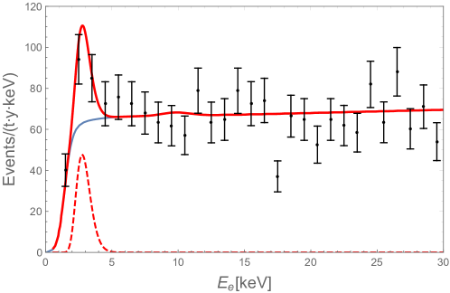
Figure 1: The differential event rate (solid red curve) for a benchmark point, $m_{\chi_{1}}=100\,{\rm GeV}$, $\alpha_{X}=3.59\times 10^{-3}$, $\epsilon=1.14\times 10^{-9}$, $\delta=2.8\,{\rm keV}$, and $m_{Z^{\prime}}=10^{-4}\,{\rm eV}$. The dashed curve is the contribution of the NP signal only. The experimental data and the background blue curve are extracted from Aprile:2020tmw .

6 Conclusions

Although the existence of dark matter is well-established, its particle nature is almost unknown. The small scale problem and the recent observation of the excess in electron-recoil at XENON1T experiment may reveal the nature of dark matter. We studied a dark matter model which can address these issues while explaining its abundance in the universe.

In the model the Majorana dark matter candidate $\chi_{1}$ has its excited partner $\chi_{2}$ with mass difference $\delta\simeq 2.8$ keV. The dark mass is about $100$ GeV and it can explain the current relic density by the thermal freeze-out mechanism whose main annihilation process is $\chi_{1}\chi_{1}(\chi_{2}\chi_{2})\to Z^{\prime}Z^{\prime}$. We find that the necessary dark gauge coupling is $\alpha_{X}\sim 10^{-3}$.

The light $Z^{\prime}$ can also mediate (in)elastic scattering $\chi_{1}\chi_{1}\to\chi_{1(2)}\chi_{1(2)}$. We solve the Schrödinger equation numerically to calculate the cross sections. We get the elastic cross section large enough to explain the small scale problems $\sigma_{\rm el}/m_{\chi_{1}}\sim 1\;{\rm cm^{2}/g}$ .

The dark sector can communicate with the SM sector through kinetic mixing parameterized by $\epsilon\sim 10^{-10}$. In the current universe the rate for the up-scattering $\chi_{1}\chi_{1}\to\chi_{2}\chi_{2}$ followed by $\chi_{2}\to\chi_{1}Z^{\prime}$ can be enhanced by the small $Z^{\prime}$ mass $m_{Z^{\prime}}\ll\delta$. The energetic $Z^{\prime}$ is absorbed by the xenon atom at the XENON1T detector via the mechanism similar to the photoelectric effect. The above mentioned values of $\epsilon$ and $\delta$ can explain the spectrum and the excess event rate observed by the XENON1T.

References

• (1) S. Tulin and H.-B. Yu, Dark Matter Self-interactions and Small Scale Structure, Phys. Rept. 730 (2018) 1 [1705.02358].
• (2) D. Harvey, R. Massey, T. Kitching, A. Taylor and E. Tittley, The non-gravitational interactions of dark matter in colliding galaxy clusters, Science 347 (2015) 1462 [1503.07675].
• (3) M. Blennow, S. Clementz and J. Herrero-Garcia, Self-interacting inelastic dark matter: A viable solution to the small scale structure problems, JCAP 03 (2017) 048 [1612.06681].
• (4) XENON collaboration, Observation of Excess Electronic Recoil Events in XENON1T, Phys. Rev. D 102 (2020) 072004 [2006.09721].
• (5) K. Harigaya, Y. Nakai and M. Suzuki, Inelastic Dark Matter Electron Scattering and the XENON1T Excess, Phys. Lett. B 809 (2020) 135729 [2006.11938].
• (6) H.M. Lee, Exothermic dark matter for XENON1T excess, JHEP 01 (2021) 019 [2006.13183].
• (7) J. Bramante and N. Song, Electric But Not Eclectic: Thermal Relic Dark Matter for the XENON1T Excess, Phys. Rev. Lett. 125 (2020) 161805 [2006.14089].
• (8) H. An and D. Yang, Direct detection of freeze-in inelastic dark matter, 2006.15672.
• (9) W. Chao, Y. Gao and M.j. Jin, Pseudo-Dirac Dark Matter in XENON1T, 2006.16145.
• (10) S. Baek, J. Kim and P. Ko, XENON1T excess in local $Z_{2}$ DM models with light dark sector, Phys. Lett. B 810 (2020) 135848 [2006.16876].
• (11) H.-J. He, Y.-C. Wang and J. Zheng, EFT Approach of Inelastic Dark Matter for Xenon Electron Recoil Detection, JCAP 01 (2021) 042 [2007.04963].
• (12) D. Choudhury, S. Maharana, D. Sachdeva and V. Sahdev, Dark matter, muon anomalous magnetic moment, and the XENON1T excess, Phys. Rev. D 103 (2021) 015006 [2007.08205].
• (13) Y. Ema, F. Sala and R. Sato, Dark matter models for the 511 keV galactic line predict keV electron recoils on Earth, Eur. Phys. J. C 81 (2021) 129 [2007.09105].
• (14) D. Borah, S. Mahapatra, D. Nanda and N. Sahu, Inelastic fermion dark matter origin of xenon1t excess with muon $(g-2)$ and light neutrino mass, Phys. Lett. B 811 (2020) 135933 [2007.10754].
• (15) D. Borah, S. Mahapatra and N. Sahu, Connecting Low scale Seesaw for Neutrino Mass and Inelastic sub-GeV Dark Matter with Abelian Gauge Symmetry, 2009.06294.
• (16) A. Aboubrahim, M. Klasen and P. Nath, Xenon-1T excess as a possible signal of a sub-GeV hidden sector dark matter, 2011.08053.
• (17) H.-J. He, Y.-C. Wang and J. Zheng, GeV Scale Inelastic Dark Matter with Dark Photon Mediator via Direct Detection and Cosmological/Laboratory Constraints, 2012.05891.
• (18) M. Dutta, S. Mahapatra, D. Borah and N. Sahu, Self-interacting Inelastic Dark Matter in the light of XENON1T excess, 2101.06472.
• (19) Y. Cui, D.E. Morrissey, D. Poland and L. Randall, Candidates for Inelastic Dark Matter, JHEP 05 (2009) 076 [0901.0557].
• (20) K.S. Babu, C.F. Kolda and J. March-Russell, Implications of generalized Z - Z-prime mixing, Phys. Rev. D 57 (1998) 6788 [hep-ph/9710441].
• (21) K. Griest and D. Seckel, Three exceptions in the calculation of relic abundances, Phys. Rev. D 43 (1991) 3191.
• (22) E.W. Kolb and M.S. Turner, The Early Universe, Westview Press (1990).
• (23) S. Ershov, J. Vaagen and M. Zhukov, Modified variable phase method for the solution of coupled radial Schrodinger equations, Phys. Rev. C 84 (2011) 064308.
• (24) F. Kahlhoefer, K. Schmidt-Hoberg and S. Wild, Dark matter self-interactions from a general spin-0 mediator, JCAP 08 (2017) 003 [1704.02149].
• (25) R. Jimenez, L. Verde and S. Oh, Dark halo properties from rotation curves, Mon. Not. Roy. Astron. Soc. 339 (2003) 243 [astro-ph/0201352].
• (26) K.C.Y. Ng, R. Laha, S. Campbell, S. Horiuchi, B. Dasgupta, K. Murase et al., Resolving small-scale dark matter structures using multisource indirect detection, Phys. Rev. D 89 (2014) 083001 [1310.1915].
• (27) C.-W. Chiang and B.-Q. Lu, Evidence of a simple dark sector from XENON1T excess, Phys. Rev. D 102 (2020) 123006 [2007.06401].
• (28) M. Berger, J. Hubbell, S. Seltzer, J. Chang, J. Coursey, R. Sukumar et al., “XCOM: Photon cross sections database.” http://www.nist.gov/pml/data/xcom/index.cfm, 2010. https://dx.doi.org/10.18434/T48G6X.
• (29) J. Jaeckel, A force beyond the Standard Model - Status of the quest for hidden photons, Frascati Phys. Ser. 56 (2012) 172 [1303.1821].
• (30) H. An, M. Pospelov and J. Pradler, Dark Matter Detectors as Dark Photon Helioscopes, Phys. Rev. Lett. 111 (2013) 041302 [1304.3461].