Cosmic acceleration with bulk viscosity in modified $f(Q)$ gravity

Abstract

In this article, we have investigated the role of bulk viscosity to study the accelerated expansion of the universe in the framework of modified $f(Q)$ gravity. The gravitational action in this modified gravity theory has the form $f(Q)$, where $Q$ denote the non-metricity scalar. In the present manuscript, we have considered a bulk viscous matter-dominated cosmological model with the bulk viscosity coefficient of the form $\xi=\xi_{0}+\xi_{1}H+\xi_{2}\left(\frac{\dot{H}}{H}+H\right)$ which is proportional to the velocity and acceleration of the expanding universe. Two sets of limiting conditions on the bulk viscous parameters $\xi_{0},$ $\xi_{1},$ $\xi_{2}$ and model parameter $\alpha$ arose here out of which one condition favours the present scenario of cosmic acceleration with a phase transition and corresponds to the universe with a Big Bang origin. Moreover, we have discussed the cosmological behaviour of some geometrical parameters. Then, we have obtained the best fitting values of the model parameters $\xi_{0},$ $\xi_{1},$ $\xi_{2}$ and $\alpha$ by constraining our model with updated Hubble datasets consisting of $57$ data points and recently released Pantheon datasets consisting of $1048$ data points which show that our obtained model has good compatibility with observations. Further, we have also included the Baryon Acoustic Oscillation (BAO) datasets of six data points with the Hubble & Pantheon datasets and obtained slightly different values of the model parameters. Finally, we have analyzed our model with the statefinder diagnostic analysis and found some interesting results and are discussed in details.

I Introduction

In the year 1915, Albert Einstein proposed the General Theory of Relativity (GR). In the Solar System tests, GR is extremely successful as yet, but GR does not give the final word to all gravity occurrences so far. Over the last two decades, a convergence of several cosmological observations indicate that our Universe is going through a period of accelerated expansion. The observational data on type Ia Supernovae have shown that the current universe is accelerating [1, 2]. The observational evidence such as Baryon Acoustic Oscillations (BAO) [3, 4], large scale structure [6, 7], galaxy redshift survey [5] and Cosmic Microwave Background Radiations (CMBR) [8, 9] strongly support this accelerating expansion. The observed late-time acceleration of the Universe is one of the premier mysteries of theoretical physics and the responsible mechanism for this accelerating expansion is still an open question. Plenty of models have been proposed in the literature to describe this recent acceleration. Basically, there are two approaches to interpret this recent acceleration of the universe. The first approach is the assumption of the existence of mysterious force with high negative pressure so-called dark energy (DE) as responsible for the current acceleration of the universe. The simplest candidate for dark energy is the cosmological constant $\Lambda$ (or vacuum energy) i.e. the fluid responsible for such an effective negative pressure with constant energy density. This model is characterized by the constant equation of state (EoS) parameter $\omega_{\Lambda}=-1$ and known as $\Lambda$CDM model [10, 11]. Even though this model agrees considerably well with observational data, it is faced with some strong problems. Of these, the two major drawbacks are the cosmic coincidence problem and the fine-tuning problem [12]. In today’s universe, the density of dark energy and the density of non-relativistic matter happen to be the same order of magnitude, even though their evolution is different. This observed coincidence between the densities referred to as cosmic coincidence problem, while the fine tuning problem refers to the inconsistency between the observed value and theoretically predicted value of the cosmological constant. To overcome these problems time-varying dark energy models have been proposed in the literature like quintessence [13, 14], k-essence [15, 16] and perfect fluid models (like the Chaplygin gas model) [17, 18]. The second approach to explain the current acceleration of the universe is to modify spacetime’s geometry. We can do this by modifying the left-hand side of the Einstein equation. Modified theories of gravity are the geometrical generalizations of Einstein’s general theory of relativity in which the cosmic acceleration can be achieved by modifying the Einstein-Hilbert action of GR. Recently, modified theories of gravity have attracted the interest of cosmologists for understanding the role of dark energy. In modified gravity, the origin of dark energy is recognized as a modification of gravity. A lot of research reveals that the modified theories of gravity can explain both early and late time acceleration of the universe. Hence, there are plenty of motivations to discover theories beyond the standard formulation of GR. There are several modified theories have been proposed in the literature like $\>f(R)\>$ theory [19, 20, 21], $\>f(T)\>$ theory [22, 23, 24], $f(T,B)$ theory [25], $\>f(R,T)\>$ theory [26, 27], $f(Q,T)$ theory [28, 29], $\>f(G)\>$ theory [30], $f(R,G)$ theory [31, 32], etc. Nowadays, $f(Q)$ theories of gravity have been extremely investigated. The symmetric teleparallel gravity or $f(Q)$ gravity was introduce by J.B. Jiménez et al. [33]. The $f(Q)$ theory is also an alternative theory for GR like teleparallel gravity. In symmetric teleparallel gravity gravitational interactions are described by the non-metricity $Q$. Recently, there are several studies done in $f(Q)$ gravity. T. Harko studied the extension of symmetric teleparallel gravity [34]. S. Mandal studied energy conditions in $f(Q)$ gravity and also did a comparative study between $f(Q)$ gravity and $\Lambda$CDM [35]. Moreover, they used the cosmographic idea to constrain the Lagrangian function $f(Q)$ using the latest pantheon data [36]. An interesting investigation on $f(Q)$ gravity was done by Noemi, where he explored the signatures of non-metricity gravity in its’ fundamental level [37].

Earlier, to study inflationary epoch in the early universe bulk viscosity has been proposed in the literature without any requirement of dark energy [38, 39]. Hence, it is very natural to expect that the bulk viscosity can be responsible for the current accelerated expansion of the universe. Nowadays, several authors are attempted to explain the late-time acceleration via bulk viscosity without any dark energy constituent or cosmological constant [40, 41, 42, 43, 44, 45]. Theoretically, deviations that occur from the local thermodynamic stability can originate the bulk viscosity but a detailed mechanism for the formation of bulk viscosity is still not achievable [46]. In cosmology, when the matter content of the universe expands or contract too fast as a cosmological fluid then the effective pressure is generated to bring back the system to its thermal stability. The bulk viscosity is the manifestation of such an effective pressure [47, 48].

In cosmology, there is two main formalism for the description of bulk viscosity. The first one is the non-casual theory, where the deviation of only first-order is considered and one can find that the heat flow and viscosity propagate with infinite speed while in the second one i.e. the casual theory it propagates with finite speed. In the year 1940, Eckart proposed the non-casual theory [49]. Later, Lifshitz and Landau gave a similar theory [50]. The casual theory was developed by Israel, Hiscock and Stewart. In this theory, second-order deviation from equilibrium is considered [51, 52, 53, 54, 55]. Moreover, Eckart theory can be acquired from it as a first-order approximation. Hence, Eckart’s theory is a good approximation to the Israel theory in the limit of vanishing relaxation time. To analyze the late acceleration of the universe, the casual theory of bulk viscosity has been used. Cataldo et al. have investigated the late time acceleration using the casual theory [56]. Basically, they used an ansatz for the Hubble parameter (inspired by the Eckart theory) and they have shown the transition of the universe from the big rip singularity to the phantom behavior.

The expansion process of an accelerating universe is a collection of states that lose their thermal stability in a small fragment of time [57]. Hence, it is quite natural to consider the existence of bulk viscosity coefficient to describe the expansion of the universe. The accelerated expansion scenario of the universe (the mean stage of low redshift) can be justified by the geometrical modification in Einstein’s equation. Also, without any requirement of cosmological constant bulk viscosity can generate an acceleration. It contributes to the pressure term and applies additional pressure to drive the acceleration [58]. C. P. Singh and Pankaj Kumar has investigated the role of bulk viscosity in modified $f(R,T)$ theories of gravity [59]. S. Davood has investigated the effect of bulk viscous matter in modified $f(T)$ theories of gravity [60].

In this work, we have focused on studying the cosmic acceleration of the universe in $f(Q)$ gravity with the presence of bulk viscous fluid. The motivation of working in the non-metricity $f(Q)$ gravity is that in this framework, the motion equations are in the second-order, which is easy to solve. In f(R) gravity, an extra scalar mode appears because the model is the higher derivative theory as the Ricci scalar includes the second-order derivatives of the metric tensor. This scalar mode generates additional force, and it is often inconsistent with the Newton law observations and also for a density of a canonical scalar field $\phi$; the non-minimal coupling between geometry and the matter Lagrangian produces an additional kinetic term which is not an agreement with the stable Horndeski class [61]. Nevertheless, the non-metricity formalism overcomes the above problems, which are induced by the higher-order theory.

In this article, we analyze the matter-dominated FLRW model in the framework of modified $f(Q)$ theories of gravity and study the role of bulk viscosity in explaining the late-time acceleration of the universe. The outline of the present article is as follows. In Sec. II we present the field equation formalism in $f(Q)$ gravity. In Sec. III we describe the FLRW universe dominated with bulk viscous matter and also we derive the expression for the Hubble parameter. In Sec. IV we derive the scale factor and found two sets of limiting conditions on the coefficients of bulk viscosity which corresponds to the universe which begins with a Big Bang and then making a transition from deceleration phase to the acceleration phase. In Sec. V we show the evolution of deceleration parameter $q$. In Sec. VI we have constrained the model parameters by using Hubble data and Pantheon data sets. In Sec. VII we adopt the statefinder diagnostic pair to differentiate present bulk viscous model with other models of dark energy. Finally, in the last section Sec. VIII we briefly discuss our conclusions.

II Motion Equations in $f(Q)$ gravity

The action in a universe governed by $f(Q)$ gravity reads

$$S=\int{\frac{1}{2}f(Q)\sqrt{-g}d^{4}x}+\int{L_{m}\sqrt{-g}d^{4}x}\text{{,}}$$ (1)

where $f(Q)$ is an arbitrary function of the nonmetricity $Q$, $g$ is the determinant of the metric $g_{\mu\nu}$ and $L_{m}$ is the matter Lagrangian density.

The nonmetricity tensor is defined as

$$Q_{\lambda\mu\nu}=\nabla_{\lambda}g_{\mu\nu}$$ (2)

and its two traces are given below

$$Q_{\alpha}={Q_{\alpha}^{\mu}}_{\mu}\ \ \text{and}\ \ \tilde{Q}_{\alpha}=Q^{\mu}_{\alpha\mu}\text{.}$$ (3)

Moreover, the superpotential tensor is given by

$$4P^{\lambda}_{\mu\nu}=-Q^{\lambda}_{\mu\nu}+2Q_{({\mu^{{}^{\lambda}}}{\nu})}+(Q^{\lambda}-\tilde{Q}^{\lambda})g_{\mu\nu}-\delta^{\mu}_{({\lambda^{{}^{Q}}}\nu)}\text{.}$$ (4)

Hence, the trace of nonmetricity tensor can be obtained as

$$Q=-Q_{\lambda\mu\nu}P^{\lambda\mu\nu}\text{.}$$ (5)

Now, the definition of the energy momentum tensor for the matter is

$$T_{\mu\nu}=\frac{-2}{\sqrt{-g}}\frac{\delta(\sqrt{-g}L_{m})}{\delta g^{\mu\nu}}\text{.}$$ (6)

For notational simplicity, we define $f_{Q}=\frac{df}{dQ}$

Varying the action (1) with respect to the metric, the gravitational field equation obtained is given below

$$\frac{2}{\sqrt{-g}}\nabla_{\lambda}(\sqrt{-g}f_{Q}P^{\lambda}_{\mu\nu})+\frac{1}{2}g_{\mu\nu}f+f_{Q}(P_{\mu\lambda\beta}Q_{\nu}^{\lambda\beta}-2Q_{\lambda\beta\mu}P^{\lambda\beta}_{\nu})=-T_{\mu\nu}$$ (7)

Furthermore, by varying the action (1) with respect to the connection, one can find the following result

$$\nabla_{\mu}\nabla_{\nu}(\sqrt{-g}f_{Q}P^{\mu\nu}_{\lambda})=0\text{.}$$ (8)

III FLRW universe dominated with bulk viscous matter

We consider that the universe is described by the spatially flat Friedmann-Lemaitre-Robertson-Walker(FLRW) line element

$$ds^{2}=-dt^{2}+a^{2}(t)[dx^{2}+dy^{2}+dz^{2}]\text{.}$$ (9)

Here, $a(t)$ is the scale factor of the universe dominated with bulk viscous matter. The trace of nonmetricity tensor with respect to line element given by (9) is

$$Q=6H^{2}\text{.}$$ (10)

For a bulk viscous fluid, described by its effective pressure $\bar{p}$ and the energy density $\rho$, the energy-momentum tensor takes the form

$$T_{\mu\nu}=(\rho+\bar{p})u_{\mu}u_{\nu}+\bar{p}h_{\mu\nu}\text{,}$$ (11)

where $h_{\mu\nu}=g_{\mu\nu}+u_{\mu}u_{\nu}$ and $\bar{p}=p-3\xi H$. Here $\xi$ is the coefficient of bulk viscosity which can be a function of Hubble parameter and its derivative and the components of four-velocity $u^{\mu}$ are $u^{\mu}=(1,0)$ and $p$ is the normal pressure which is 0 for non-relativistic matter.

The Friedmann equations describing the universe dominated with bulk viscous matter are

$$3H^{2}=\frac{1}{2f_{Q}}\left(-\rho+\frac{f}{2}\right)$$ (12)

and

$$\dot{H}+3H^{2}+\frac{\dot{f_{Q}}}{f_{Q}}H=\frac{1}{2f_{Q}}\left(\bar{p}+\frac{f}{2}\right)\text{.}$$ (13)

In an accelerated expanding universe, the coefficient of viscosity should depend on velocity and acceleration. In this paper, we consider a time dependent bulk viscosity of the form [62]

$$\xi=\xi_{0}+\xi_{1}\left(\frac{\dot{a}}{a}\right)+\xi_{2}\left(\frac{{\ddot{a}}}{\dot{a}}\right)=\xi_{0}+\xi_{1}H+\xi_{2}\left(\frac{\dot{H}}{H}+H\right)\text{.}$$ (14)

It is a linear combination of three terms, first one is a constant, second one is proportional to the Hubble parameter, which indicates the dependence of the viscosity on speed, and the third one is proportional to the $\frac{\ddot{a}}{\dot{a}}$, indicating the dependence of the bulk viscosity on acceleration.

In this paper, we consider the following functional form of $f(Q)$

$$f(Q)=\alpha Q,\ \ \ \alpha\neq 0\text{.}$$ (15)

Then, for this particular choice of the function, the field equation becomes

$$\rho=-3\alpha H^{2}$$ (16)

and

$$\bar{p}=2\alpha\dot{H}+3\alpha H^{2}\text{.}$$ (17)

As we are concerned with late-time acceleration, we have considered the non-relativistic matter dominates the universe. From the Friedmann equation (17) and equation (14), we have first-order differential equation for the Hubble parameter by replacing $\frac{d}{dt}$ with $\frac{d}{dln(a)}$ via $\frac{d}{dt}=H\frac{d}{dln(a)}$

$$\frac{dH}{dln(a)}+\left(\frac{3\alpha+3\xi_{1}+3\xi_{2}}{2\alpha+3\xi_{2}}\right)H+\left(\frac{3\xi_{0}}{2\alpha+3\xi_{2}}\right)=0\text{.}$$ (18)

Now, we set

$$3\xi_{0}=\bar{\xi_{0}}H_{0},\ \ 3\xi_{1}=\bar{\xi_{1}},\ \ 3\xi_{2}=\bar{\xi_{2}}\ \ \text{and}\ \ \bar{\xi}_{12}=\bar{\xi_{1}}+\bar{\xi_{2}}\text{,}$$ (19)

where $H_{0}$ is present value of the Hubble parameter and $\bar{\xi}_{0},\ \$ $\bar{\xi}_{1},\ \$ $\bar{\xi}_{2}$ are the dimensionless bulk viscous parameters, then by using above equation (18) becomes

$$\frac{dH}{dln(a)}+\left(\frac{3\alpha+\bar{\xi}_{12}}{2\alpha+\bar{\xi_{2}}}\right)H+\left(\frac{\bar{\xi_{0}}}{2\alpha+\bar{\xi_{2}}}\right)H_{0}=0\text{.}$$ (20)

After integrating above equation we obtain the Hubble parameter as

$$H(a)=H_{0}\left[a^{-\left(\frac{3\alpha+\bar{\xi}_{12}}{2\alpha+\bar{\xi_{2}}}\right)}\left(1+\frac{\bar{\xi_{0}}}{3\alpha+\bar{\xi}_{12}}\right)-\frac{\bar{\xi_{0}}}{3\alpha+\bar{\xi}_{12}}\right]\text{.}$$ (21)

At $\bar{\xi}_{0}=\bar{\xi}_{1}=\bar{\xi}_{2}=0$, equation (21) becomes

$$H=H_{0}a^{-\frac{3}{2}}\text{.}$$ (22)

The equation (22) gives the value of the Hubble parameter in case of ordinary matter-dominated universe i.e. when all the bulk viscous parameters are $0$.
Now, by using the relation between redshift and scale factor i.e $a(t)=\frac{1}{1+z}$, in terms of redshift the Hubble parameter is given as

$$H(z)=H_{0}\left[(1+z)^{\left(\frac{3\alpha+\bar{\xi}_{12}}{2\alpha+\bar{\xi_{2}}}\right)}\left(1+\frac{\bar{\xi_{0}}}{3\alpha+\bar{\xi}_{12}}\right)-\frac{\bar{\xi_{0}}}{3\alpha+\bar{\xi}_{12}}\right]\text{.}$$ (23)

IV Scale factor

Now, using the definition of Hubble parameter, the equation (21) becomes

$$\frac{1}{a}\frac{da}{dt}=H_{0}\left[a^{-\left(\frac{3\alpha+\bar{\xi}_{12}}{2\alpha+\bar{\xi_{2}}}\right)}\left(1+\frac{\bar{\xi_{0}}}{3\alpha+\bar{\xi}_{12}}\right)-\frac{\bar{\xi_{0}}}{3\alpha+\bar{\xi}_{12}}\right]\text{.}$$ (24)

On integrating the above equation we get the scale factor

$$a(t)=\left[\frac{3\alpha+\bar{\xi}_{12}+\bar{\xi}_{0}}{\bar{\xi}_{0}}-\left(\frac{3\alpha+\bar{\xi}_{12}}{\bar{\xi}_{0}}\right)e^{-H_{0}(t-t_{0})\frac{\bar{\xi}_{0}}{2\alpha+\bar{\xi}_{2}}}\right]^{\frac{2\alpha+\bar{\xi}_{2}}{3\alpha+\bar{\xi}_{12}}}\text{,}$$ (25)

where $t_{0}$ is the present cosmic time.

Now, let $y=H_{0}(t-t_{0})$ , then the second order derivative of $a(t)$ with respect to $y$ is

$$\frac{d^{2}a}{dy^{2}}=\frac{e^{\frac{-\bar{\xi}_{0}y}{2\alpha+\bar{\xi}_{2}}}}{2\alpha+\bar{\xi}_{2}}\left(-(\bar{\xi}_{0}+\bar{\xi}_{12}+3\alpha)+(2\alpha+\bar{\xi}_{2})e^{\frac{-\bar{\xi}_{0}y}{2\alpha+\bar{\xi}_{2}}}\right)\times\left[\frac{\bar{\xi}_{0}+\bar{\xi}_{12}+3\alpha-(3\alpha+\bar{\xi}_{12})e^{\frac{-\bar{\xi}_{0}y}{2\alpha+\bar{\xi}_{2}}}}{\bar{\xi}_{0}}\right]^{\frac{-2(2\alpha+\bar{\xi}_{1})-\bar{\xi}_{2}}{3\alpha+\bar{\xi}_{12}}}\text{.}$$ (26)

From the above expression it is clear that we have two limiting conditions based on the values of $\bar{\xi}_{0},$ $\bar{\xi}_{1}$ and $\bar{\xi}_{2}$. By equation (16) and the fact that density of ordinary matter in the universe is always positive, so we must have $\alpha<0$. Assuming, $\alpha=-\bar{\alpha}$ where $\bar{\alpha}>0$, these two limiting conditions are

$$\bar{\xi}_{0}>0,\text{ }\bar{\xi}_{12}<3\bar{\alpha},\text{ }\bar{\xi}_{2}<2\bar{\alpha},\text{ }\bar{\xi}_{0}+\bar{\xi}_{12}<3\bar{\alpha}$$ (27)

and

$$\bar{\xi}_{0}<0,\text{ }\bar{\xi}_{12}>3\bar{\alpha},\text{ }\bar{\xi}_{2}>2\bar{\alpha},\text{ }\bar{\xi}_{0}+\bar{\xi}_{12}>3\bar{\alpha}\text{.}$$ (28)

These two limiting condition implies that the universe experienced a deceleration phase at early times and then making a transition into the accelerated phase in the latter times. If we place $\bar{\xi}_{0}+\bar{\xi}_{12}>3\bar{\alpha}$ and $\bar{\xi}_{0}+\bar{\xi}_{12}<3\bar{\alpha}$ in the first and second limiting condition respectively, then the universe will experience an everlasting accelerated expansion.

V Deceleration parameter

The deceleration parameter is defined as

$$q=-\frac{a\ddot{a}}{\dot{a}^{2}}=-\frac{\ddot{a}}{a}\frac{1}{H^{2}}\text{.}$$ (29)

From the Friedmann equation (17) one can obtain

$$\frac{\ddot{a}}{a}=-\frac{1}{2\alpha}\left[\alpha H^{2}+3H\left(\xi_{0}+\xi_{1}H+\xi_{2}\left(\frac{\dot{H}}{H}+H\right)\right)\right]\text{.}$$ (30)

Using the equation (19) the deceleration parameter becomes

$$q=\frac{1}{2\alpha}\left[\bar{\xi}_{0}\frac{H_{0}}{H}+\left(\bar{\xi}_{12}+\alpha\right)+\bar{\xi}_{2}\frac{\dot{H}}{H^{2}}\right]\text{.}$$ (31)

Now, using the value of Hubble parameter given by equation (21) and equations (17)-(20), the equation (31) becomes

$$q(a)=\frac{1}{2\alpha+\bar{\xi}_{2}}\left[\bar{\xi}_{1}+\alpha+\frac{\bar{\xi}_{0}}{a^{-\left(\frac{3\alpha+\bar{\xi}_{12}}{2\alpha+\bar{\xi}_{2}}\right)}\left[1+\frac{\bar{\xi}_{0}}{3\alpha+\bar{\xi}_{12}}\right]-\frac{\bar{\xi}_{0}}{3\alpha+\bar{\xi}_{12}}}\right]\text{.}$$ (32)

Now, by using relation between redshift and scale factor i.e., $a(t)=\frac{1}{1+z}$, in terms of redshift deceleration parameter is given as

$$q(z)=\frac{1}{2\alpha+\bar{\xi}_{2}}\left[\bar{\xi}_{1}+\alpha+\frac{\bar{\xi}_{0}}{(1+z)^{\left(\frac{3\alpha+\bar{\xi}_{12}}{2\alpha+\bar{\xi}_{2}}\right)}\left[1+\frac{\bar{\xi}_{0}}{3\alpha+\bar{\xi}_{12}}\right]-\frac{\bar{\xi}_{0}}{3\alpha+\bar{\xi}_{12}}}\right]$$ (33)

The present value of deceleration parameter i.e., the value of $q$ at $z=0$ or $a=1$ is,

$$q_{0}=\frac{\alpha+\bar{\xi}_{0}+\bar{\xi}_{1}}{2\alpha+\bar{\xi}_{2}}\text{.}$$ (34)

If the value of all bulk viscous parameters are 0, then the deceleration parameter becomes $q=\frac{1}{2}$ which correspond to a matter dominated decelerating universe with null bulk viscosity. For the two sets of limiting conditions based on the dimensionless bulk viscous parameter, the variation of deceleration parameter with respect to redshift $z$ can be plotted as shown in Figs. 1 and 2.

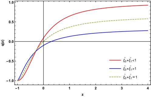
Figure 1: Variation of the deceleration parameter with redshift $z$ for the first limiting conditions $\bar{\xi}_{0}>0,\bar{\xi}_{12}<3,\bar{\xi}_{2}<2,\bar{\xi}_{0}+\bar{\xi}_{12}<3$. Here, we took $\alpha=-1$ i.e., $\bar{\alpha}=1$. $q$ enters the negative region in the recent past if $\bar{\xi}_{0}+\bar{\xi}_{1}>1$, at present if $\bar{\xi}_{0}+\bar{\xi}_{1}=1$ and in the future if $\bar{\xi}_{0}+\bar{\xi}_{1}<1$. For Red, Blue and Green plots the value of $(\bar{\xi}_{0},\bar{\xi}_{1},\bar{\xi}_{2})$ are $(0.9,0.01,1),(0.45,0.65,1),(0.65,0.35,1)$ respectively.

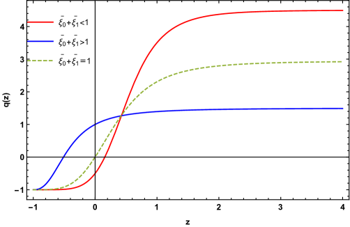
Figure 2: Variation of the deceleration parameter with redshift $z$ for the second limiting conditions $\bar{\xi}_{0}<0,\bar{\xi}_{12}>3,\bar{\xi}_{2}>2,\bar{\xi}_{0}+\bar{\xi}_{12}>3$. Here, we took $\alpha=-1$ i.e., $\bar{\alpha}=1$. $q$ enters the negative region in the recent past if $\bar{\xi}_{0}+\bar{\xi}_{1}<1$, at present if $\bar{\xi}_{0}+\bar{\xi}_{1}=1$ and in the future if $\bar{\xi}_{0}+\bar{\xi}_{1}>1$. For Red, Blue and Green plots the value of $(\bar{\xi}_{0},\bar{\xi}_{1},\bar{\xi}_{2})$ are $(-0.5,1.45,2.1),(-0.5,2.5,3),(-0.5,1.5,2.17)$ respectively

From the above figures of $q(z)\sim z$, we can see that, only first limiting condition with $\bar{\xi}_{0}+\bar{\xi}_{1}>1$ (blue line in Fig. 1 shows a phase transition from early deceleration to present acceleration and second limiting condition is not be suitable to discuss the present observational scenario. Also the first limiting condition with $\bar{\xi}_{0}+\bar{\xi}_{1}=1$ and $\bar{\xi}_{0}+\bar{\xi}_{1}<1$, which can be inferred from the following plots of Hubble parameter $H(z)\sim z$ as shown in Figs. 3 and 4.

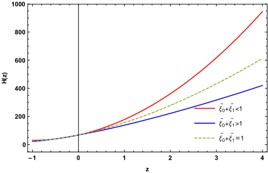
Figure 3: Variation of the Hubble parameter with redshift $z$ for the first limiting conditions $\bar{\xi}_{0}>0,\bar{\xi}_{12}<3,\bar{\xi}_{2}<2,\bar{\xi}_{0}+\bar{\xi}_{12}<3$. Here we took $\alpha=-1$ i.e., $\bar{\alpha}=1$. For Red, Blue and Green plots the value of $(\bar{\xi}_{0},\bar{\xi}_{1},\bar{\xi}_{2})$ are $(0.9,0.01,1),(0.45,0.65,1),(0.65,0.35,1)$ respectively.

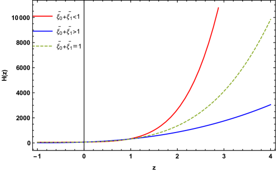
Figure 4: Variation of the Hubble parameter with redshift $z$ for the second limiting conditions $\bar{\xi}_{0}<0,\bar{\xi}_{12}>3,\bar{\xi}_{2}>2,\bar{\xi}_{0}+\bar{\xi}_{12}>3$. Here we took $\alpha=-1$ i.e., $\bar{\alpha}=1$. For Red, Blue and Green plots the value of $(\bar{\xi}_{0},\bar{\xi}_{1},\bar{\xi}_{2})$ are $(-0.5,1.45,2.1),(-0.5,2.5,3),(-0.5,1.5,2.17)$ respectively

With a discussion of the geometrical behavior of our obtained model, we shall now try to find out suitable numerical values of the model parameters consistent with the present observations. We only consider the first limiting condition for our further analysis.

VI Best fit values of model parameters from observation

We have found an exact solution of the Einstein field equations with the bulk viscous matter in $f(Q)$ gravity having four model parameters $\alpha$, $\xi_{0}$, $\xi_{1}$ and $\xi_{2}$. We must discuss the approximate values of these model parameters describing well the present universe through some observational datasets. To obtain the best fit values of these model parameters, we have used mainly two datasets namely, the Hubble datasets containing $57$ data points and the Pantheon datasets containing $1048$ datasets. Furthermore, we have discussed our results together with the Baryon Acoustic oscillations (BAO) datasets. To constrain the model parameters with the above discussed datasets, we have used the Python’s Scipy optimization technique. First, we have estimated the global minima for the Hubble function in equation (23). For the numerical analysis, we employ the Python’s emcee library and consider a Gaussian prior with above estimates as means and a fixed $\sigma=1.0$ as dispersion. The idea behind the analysis is to check the parameter space in the neighborhood of the local minima. More about the Hubble datasets, Pantheon datasets and BAO datasets and methodology are discussed below in some detail and finally, the results are discussed as 2-dimensional contour plots with $1-\sigma$ & $2-\sigma$ errors.

VI.1 H(z) datasets

We are familiar with the well known cosmological principle which assumes that on the large scale, our universe is homogeneous and isotropic. This principle is the backbone of modern cosmology. In the last few decades this principle had been tested several times and have been supported by many cosmological observations. In the study of observational cosmology, the expansion scenario of the universe be directly investigated by the Hubble parameter i.e. $H=\frac{\dot{a}}{a}$ where $\dot{a}$ represents derivative of cosmic scale factor $a$ with respect to cosmic time $t$. The Hubble parameter as a function of redshift can be expressed as $H(z)$ $=-\frac{1}{1+z}\frac{dz}{dt}$, where $dz$ is acquired from the spectroscopic surveys and therefore a measurement of $dt$ furnishes the model independent value of the Hubble parameter. In general, there are two well known methods that are used to measure the value of the Hubble parameter values $H(z)$ at some definite redshift. The first one is the extraction of $H(z)$ from line-of-sight BAO data and another one is the differential age method [63]-[81]. In this manuscript, we have taken an updated set of $57$ data points. In this set of $57$ Hubble data points, $31$ points measured via the method of differential age (DA) and remaining $26$ points through BAO and other methods in the range of redshift given as $0.07\leqslant z\leqslant 2.42$ [82]. Furthermore, we have taken $H_{0}=69$ $Km/s/Mpc$ for our analysis . To find out the mean values of the model parameters $\alpha$, $\xi_{0}$, $\xi_{1}$ and $\xi_{2}$ (which is equivalent to the maximum likelihood analysis), we have taken the chi-square function as,

$$\chi_{H}^{2}(\alpha,\xi_{0},\xi_{1},\xi_{2})=\sum\limits_{i=1}^{57}\frac{[H_{th}(z_{i},\alpha,\xi_{0},\xi_{1},\xi_{2})-H_{obs}(z_{i})]^{2}}{\sigma_{H(z_{i})}^{2}},$$ (35)

where the theoretical value of Hubble parameter is represented by $H_{th}$ and the observed value by $H_{obs}$ and $\sigma_{H(z_{i})}$ represents the standard error in the observed value of $H$. The $57$ points of Hubble parameter values $H(z)$ with errors $\sigma_{H}$ from differential age ($31$ points) method and BAO and other ($26$ points) methods are tabulated in Table-1 with references.

Table-1: 57 points of $H(z)$ datasets
31 points from DA method
$z$	$H(z)$	$\sigma_{H}$	Ref.	$z$	$H(z)$	$\sigma_{H}$	Ref.
$0.070$	$69$	$19.6$	[63]	$0.4783$	$80$	$99$	[67]
$0.90$	$69$	$12$	[64]	$0.480$	$97$	$62$	[63]
$0.120$	$68.6$	$26.2$	[63]	$0.593$	$104$	$13$	[65]
$0.170$	$83$	$8$	[64]	$0.6797$	$92$	$8$	[65]
$0.1791$	$75$	$4$	[65]	$0.7812$	$105$	$12$	[65]
$0.1993$	$75$	$5$	[65]	$0.8754$	$125$	$17$	[65]
$0.200$	$72.9$	$29.6$	[66]	$0.880$	$90$	$40$	[63]
$0.270$	$77$	$14$	[64]	$0.900$	$117$	$23$	[64]
$0.280$	$88.8$	$36.6$	[66]	$1.037$	$154$	$20$	[65]
$0.3519$	$83$	$14$	[65]	$1.300$	$168$	$17$	[64]
$0.3802$	$83$	$13.5$	[67]	$1.363$	$160$	$33.6$	[69]
$0.400$	$95$	$17$	[64]	$1.430$	$177$	$18$	[64]
$0.4004$	$77$	$10.2$	[67]	$1.530$	$140$	$14$	[64]
$0.4247$	$87.1$	$11.2$	[67]	$1.750$	$202$	$40$	[64]
$0.4497$	$92.8$	$12.9$	[67]	$1.965$	$186.5$	$50.4$	[69]
$0.470$	$89$	$34$	[68]
26 points from BAO & other method
$z$	$H(z)$	$\sigma_{H}$	Ref.	$z$	$H(z)$	$\sigma_{H}$	Ref.
$0.24$	$79.69$	$2.99$	[70]	$0.52$	$94.35$	$2.64$	[72]
$0.30$	$81.7$	$6.22$	[71]	$0.56$	$93.34$	$2.3$	[72]
$0.31$	$78.18$	$4.74$	[72]	$0.57$	$87.6$	$7.8$	[76]
$0.34$	$83.8$	$3.66$	[70]	$0.57$	$96.8$	$3.4$	[77]
$0.35$	$82.7$	$9.1$	[73]	$0.59$	$98.48$	$3.18$	[72]
$0.36$	$79.94$	$3.38$	[72]	$0.60$	$87.9$	$6.1$	[75]
$0.38$	$81.5$	$1.9$	[74]	$0.61$	$97.3$	$2.1$	[74]
$0.40$	$82.04$	$2.03$	[72]	$0.64$	$98.82$	$2.98$	[72]
$0.43$	$86.45$	$3.97$	[70]	$0.73$	$97.3$	$7.0$	[75]
$0.44$	$82.6$	$7.8$	[75]	$2.30$	$224$	$8.6$	[78]
$0.44$	$84.81$	$1.83$	[72]	$2.33$	$224$	$8$	[79]
$0.48$	$87.79$	$2.03$	[72]	$2.34$	$222$	$8.5$	[80]
$0.51$	$90.4$	$1.9$	[74]	$2.36$	$226$	$9.3$	[81]

Using the above datasets, we have estimated the best fit values of the model parameters $\alpha$, $\xi_{0}$, $\xi_{1}$ and $\xi_{2}$ as and is shown in the following plot 5 as 2-d contour sub-plots with $1-\sigma$ & $2-\sigma$ errors. The best fit values are obtained as $\alpha=-1.03_{-0.55}^{+0.52}$, $\xi_{0}=1.54_{-0.79}^{+0.83}$, $\xi_{1}=0.08_{-0.49}^{+0.49}$ and $\xi_{2}=0.66_{-0.83}^{+0.82}$ with the $57$ points of Hubble datasets as given in Table-1. Also, we have shown the error bar plot for the discussed Hubble datasets and is shown in the following plot 6 together with our obtained model compared with the $\Lambda$CDM model (with $\Omega_{m0}=0.3$ and $\Omega_{\Lambda 0}=0.7$). The plot shows nice fit of our model to the observational Hubble datasets.

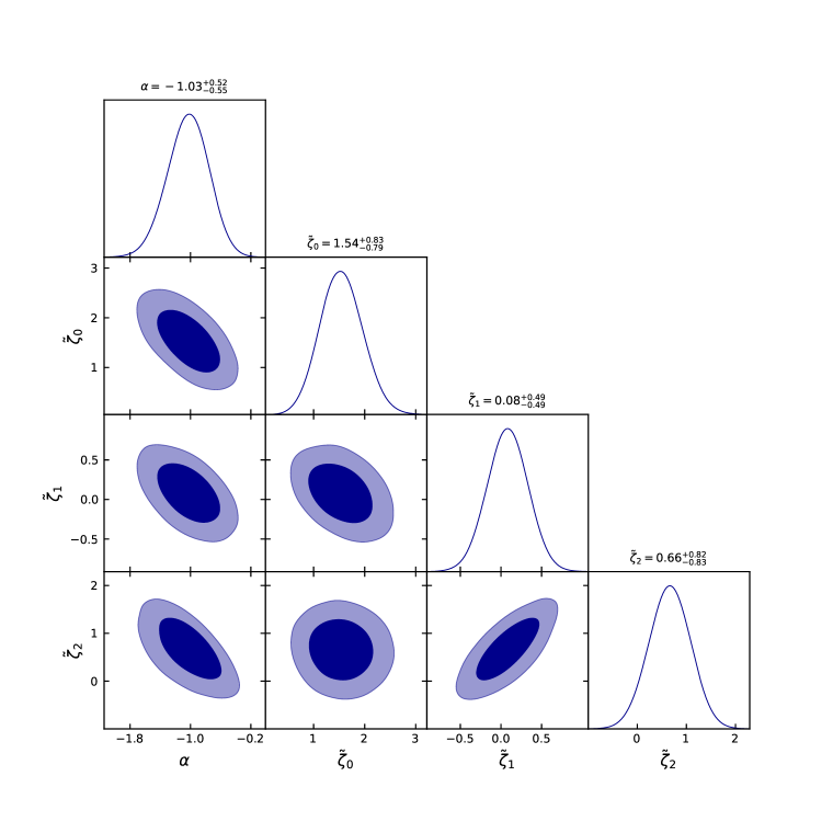
Figure 5: The plot shows the 2-d contour plots of the model parameters with $1-\sigma$ and $2-\sigma$ errors and also shows the best fit values of the model parameters $\alpha$, $\xi_{0}$, $\xi_{1}$ and $\xi_{2}$ obtained from the $57$ points of Hubble datasets.

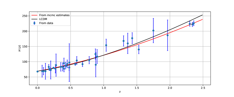
Figure 6: The plot shows the plot of Hubble function $H(z)$ vs. redshift $z$ for our model shown in red line which shows nice fit to the $57$ points of the Hubble datasets shown in dots with it’s error bars and also compared to the $\Lambda$CDM model shown in black solid line with $\Omega_{m0}=0.3$ & $\Omega_{\Lambda 0}=0.7$.

VI.2 Pantheon datasets

Initially, the observational studies on supernovae of the golden sample of $50$ points of type Ia suggested that our universe is in an accelerating phase of expansion. After the result, the studies on more and more samples of supernovae datasets increased during the past two decades. Recently, the latest sample of supernovae of type Ia datasets are released containing $1048$ data points. In this article, we have used this set of datasets known as Pantheon datasets [83] with $1048$ samples of spectroscopically confirmed SNe Ia covering the range in the redshift range $0.01<z<2.26$. In the redshift range $0<z_{i}\leq 1.41$, these data points gives the estimation of the distance moduli $\mu_{i}=\mu_{i}^{obs}$. Here, we fit our model parameters of the obtained model, comparing the theoretical $\mu_{i}^{th}$ value and the observed $\mu_{i}^{obs}$ value of the distance modulus. The distance moduli which are the logarithms given as $\mu_{i}^{th}=\mu(D_{L})=m-M=5\log_{10}(D_{L})+\mu_{0}$, where $m$ and $M$ represents apparent and absolute magnitudes and $\mu_{0}=5\log\left(H_{0}^{-1}/Mpc\right)+25$ is the marginalized nuisance parameter. The luminosity distance is taken to be,

$$D_{l}(z) = \frac{c(1+z)}{H_{0}}S_{k}\left(H_{0}\int_{0}^{z}\frac{1}{H(z^{\ast})}dz^{\ast}\right),$$

$$\text{where }S_{k}(x) = \left\{\begin{array}[]{c}\sinh(x\sqrt{\Omega_{k}})/\Omega_{k}\text{, }\Omega_{k}>0\\ x\text{, \ \ \ \ \ \ \ \ \ \ \ \ \ \ \ \ \ \ \ \ \ \ \ }\Omega_{k}=0\\ \sin x\sqrt{\left|\Omega_{k}\right|})/\left|\Omega_{k}\right|\text{, }\Omega_{k}<0\end{array}\right..$$

Here, $\Omega_{k}=0$ (flat space-time). We have calculated distance $D_{L}(z)$ and corresponding chi square function that measures difference between predictions of our model and the SN Ia observational data. The $\chi_{SN}^{2}$ function for the Pantheon datasets is taken to be,

$$\chi_{SN}^{2}(\mu_{0},\alpha,\xi_{0},\xi_{1},\xi_{2})=\sum\limits_{i=1}^{1048}\frac{[\mu^{th}(\mu_{0},z_{i},\alpha,\xi_{0},\xi_{1},\xi_{2})-\mu^{obs}(z_{i})]^{2}}{\sigma_{\mu(z_{i})}^{2}},$$ (37)

$\sigma_{\mu(z_{i})}^{2}$ is the standard error in the observed value. After marginalizing $\mu_{0}$, the chi square function is written as,

$\qquad\qquad\qquad\qquad\qquad\qquad\qquad\qquad\chi_{SN}^{2}(\alpha,\xi_{0},\xi_{1},\xi_{2})=A(\alpha,\xi_{0},\xi_{1},\xi_{2})-[B(\alpha,\xi_{0},\xi_{1},\xi_{2})]^{2}/C(\alpha,\xi_{0},\xi_{1},\xi_{2})$

where

$\qquad\qquad\qquad\qquad\qquad\qquad\qquad\qquad A(\alpha,\xi_{0},\xi_{1},\xi_{2})=\sum\limits_{i=1}^{1048}\frac{[\mu^{th}(\mu_{0}=0,z_{i},\alpha,\xi_{0},\xi_{1},\xi_{2})-\mu^{obs}(z_{i})]^{2}}{\sigma_{\mu(z_{i})}^{2}},$

$\qquad\qquad\qquad\qquad\qquad\qquad\qquad\qquad B(\alpha,\xi_{0},\xi_{1},\xi_{2})=\sum\limits_{i=1}^{1048}\frac{[\mu^{th}(\mu_{0}=0,z_{i},\alpha,\xi_{0},\xi_{1},\xi_{2})-\mu^{obs}(z_{i})]^{2}}{\sigma_{\mu(z_{i})}^{2}},$

$\qquad\qquad\qquad\qquad\qquad\qquad\qquad\qquad C(\alpha,\xi_{0},\xi_{1},\xi_{2})=\sum\limits_{i=1}^{1048}\frac{1}{\sigma_{\mu(z_{i})}^{2}}$.

Using the above Pantheon datasets, we have estimated the best fit values of the model parameters $\alpha$, $\xi_{0}$, $\xi_{1}$ and $\xi_{2}$ and is shown in the following plot 7 as 2-d contour sub-plots with $1-\sigma$ & $2-\sigma$ errors. The best fit values are obtained as $\alpha=-1.33_{-0.43}^{+0.45}$, $\xi_{0}=0.10_{-0.12}^{+0.21}$, $\xi_{1}=1.81_{-0.87}^{+0.91}$ and $\xi_{2}=2.08_{-0.96}^{+0.91}$ with $1048$ points of Pantheon datasets. Also, we have shown the error bar plot for the discussed Pantheon datasets and is shown in the following plot 8 together with our obtained model compared with the $\Lambda$CDM model (with $\Omega_{m0}=0.3$ and $\Omega_{\Lambda 0}=0.7$). The plot shows nice fit of our model to the observational Pantheon datasets.

Figure 7: The plot shows the best fit values of the model parameters $\alpha$, $\xi_{0}$, $\xi_{1}$ and $\xi_{2}$ obtained w.r.t to the $1048$ points of Pantheon datasets at $1-\sigma$ and $2-\sigma$ confidence level.

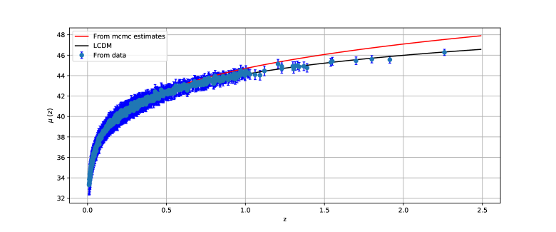
Figure 8: The plot shows the plot of distance modulus $\mu(z)$ vs. redshift $z$ for our model shown in red line which shows nice fit to the $1048$ points of the Pantheon datasets shown in dots with it’s error bars.

VI.3 BAO datasets

In the study of the Early Universe baryons, photons and dark matter come into picture and act as a single fluid coupled tightly through the Thompson scattering) but do not collapse under gravity and oscillate due to the large pressure of photons. Baryonic acoustic oscillations is an analysis that discusses these oscillations in the early Universe. The characteristic scale of BAO is governed by the sound horizon $r_{s}$ at the photon decoupling epoch $z_{\ast}$ and is given by the following relation,

$$r_{s}(z_{\ast})=\frac{c}{\sqrt{3}}\int_{0}^{\frac{1}{1+z_{\ast}}}\frac{da}{a^{2}H(a)\sqrt{1+(3\Omega_{0b}/4\Omega_{0\gamma})a}},$$

where $\Omega_{0b}$ and $\Omega_{0\gamma}$ are respectively referred to baryon density and photon density at present time.

The angular diameter distance $D_{A}$ and the Hubble expansion rate $H$ as a function of $z$ are derived using the BAO sound horizon scale. If the measured angular separation of the BAO feature is denoted by $\triangle\theta$ in the 2 point correlation function of the galaxy distribution on the sky and if the measured redshift separation of the BAO feature is denoted by $\triangle z$in same the 2 point correlation function along the line of sight then we have the relation, $\triangle\theta=\frac{r_{s}}{d_{A}(z)}$where $d_{A}(z)=\int_{0}^{z}\frac{dz^{\prime}}{H(z^{\prime})}$and $\triangle z=H(z)r_{s}$. Here, in this work, a simple BAO datasets of six points for $d_{A}(z_{\ast})/D_{V}(z_{BAO})$ is considered from the references [84, 85, 86, 87, 88, 89], where the photon decoupling redshift is taken as $z_{\ast}\approx 1091$and $d_{A}(z)$ is the co-moving angular diameter distance together with the dilation scale $D_{V}(z)=\left(d_{A}(z)^{2}z/H(z)\right)^{1/3}$. The following table-2 shows the six points of the BAO datasets,

Table-2: Values of $d_{A}(z_{\ast})/D_{V}(z_{BAO})$ for distinct values of $z_{BAO}$
$z_{BAO}$	$0.106$	$0.2$	$0.35$	$0.44$	$0.6$	$0.73$
$\frac{d_{A}(z_{\ast})}{D_{V}(z_{BAO})}$	$30.95\pm 1.46$	$17.55\pm 0.60$	$10.11\pm 0.37$	$8.44\pm 0.67$	$6.69\pm 0.33$	$5.45\pm 0.31$

.

Also, the chi square function for BAO is given by [89],

$$\chi_{BAO}^{2}=X^{T}C^{-1}X\,,$$ (38)

where

$$X=\left(\begin{array}[]{c}\frac{d_{A}(z_{\star})}{D_{V}(0.106)}-30.95\\ \frac{d_{A}(z_{\star})}{D_{V}(0.2)}-17.55\\ \frac{d_{A}(z_{\star})}{D_{V}(0.35)}-10.11\\ \frac{d_{A}(z_{\star})}{D_{V}(0.44)}-8.44\\ \frac{d_{A}(z_{\star})}{D_{V}(0.6)}-6.69\\ \frac{d_{A}(z_{\star})}{D_{V}(0.73)}-5.45\end{array}\right)\,,$$

and the inverse covariance matrix $C^{-1}$ is defined in [89].

$$C^{-1}=\left(\begin{array}[]{cccccc}0.48435&-0.101383&-0.164945&-0.0305703&-0.097874&-0.106738\\ -0.101383&3.2882&-2.45497&-0.0787898&-0.252254&-0.2751\\ -0.164945&-2.454987&9.55916&-0.128187&-0.410404&-0.447574\\ -0.0305703&-0.0787898&-0.128187&2.78728&-2.75632&1.16437\\ -0.097874&-0.252254&-0.410404&-2.75632&14.9245&-7.32441\\ -0.106738&-0.2751&-0.447574&1.16437&-7.32441&14.5022\end{array}\right)\,.$$

Including these six data points of the BAO datasets with the Hubble datasets and combine the above results of Hubble constrained values, we obtain the values of the model parameters as, $\alpha=-1.06_{-0.82}^{+0.34}$, $\xi_{0}=2.25_{-1.7}^{+0.37}$, $\xi_{1}=-0.08_{-0.96}^{+1.1}$ and $\xi_{2}=0.7_{-1.1}^{+1.1}$. Similarly, including these six data points of the BAO datasets with the Pantheon datasets and combine the above results of Panteon constrained values, we obtain the values of the model parameters as, $\alpha=-1.65_{-0.25}^{+0.85}$, $\xi_{0}=0.86_{-1.1}^{+0.29}$, $\xi_{1}=-1.90_{-0.99}^{+0.97}$ and $\xi_{2}=1.93_{-0.91}^{+1.2}$. The combined results are shown as 2-d contour sub-plots with $1-\sigma$ & $2-\sigma$ errors in the following plots 9 and 10.

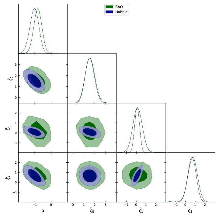
Figure 9: The plot shows the 2-d contour plots of the model parameters with $1-\sigma$ and $2-\sigma$ errors and also shows the best fit values of the model parameters $\alpha$, $\xi_{0}$, $\xi_{1}$ and $\xi_{2}$ obtained from the $57$ points of Hubble datasets together with six points of BAO datasets.

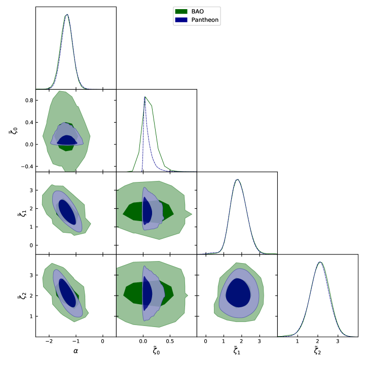
Figure 10: The plot shows the best fit values of the model parameters $\alpha$, $\xi_{0}$, $\xi_{1}$ and $\xi_{2}$ obtained w.r.t to the $1048$ points of Pantheon datasets together with six points of BAO datasets at $1-\sigma$ and $2-\sigma$ confidence level.

VII Statefinder Diagnostic

It is well-known that the deceleration parameter $q$ and the Hubble parameter $H$ are the oldest geometric variable. During the last few decades, plenty of DE (Dark Energy) models have been proposed and the remarkable growth in the precision of observational data both motivate us to go beyond these two parameters. In this direction, a new pair of geometrical quantities have been proposed by V. Sahni et al. [90] called statefinder diagnostic parameters $(r,s)$. The state finder parameters investigate the expansion dynamics through second and third derivatives of the cosmic scale factor which is a natural succeeding step beyond the parameters $H$ and $q$. These parameters are defined as follows

$$r=\frac{\dddot{a}}{aH^{3}}$$ (39)

and

$$s=\frac{r-1}{3(q-\frac{1}{2})}\text{.}$$ (40)

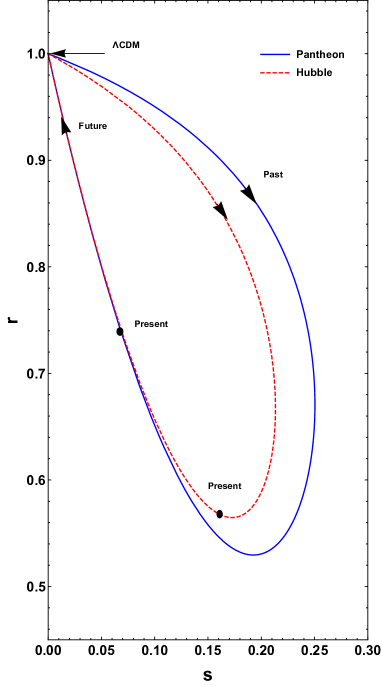
Figure 11: The evolution trajectories of the given model in $s-r$ plane corresponding to the values of model parameters constrained by the Hubble and Pantheon datasets.

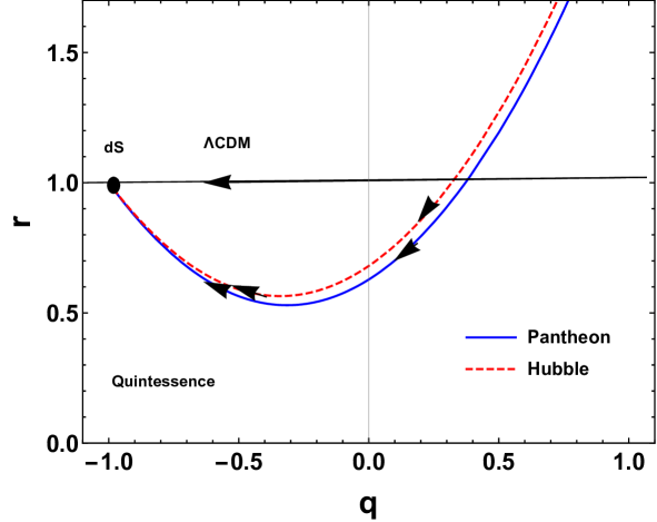
Figure 12: The evolution trajectories of the given model in $q-r$ plane corresponding to the values of model parameters constrained by the Hubble and Pantheon datasets.

The fixed point $(s,r)=(0,1)$ in the $s-r$ diagram 11 shows the spatially flat $\Lambda$CDM model and $(q,r)=(-1,1)$ shows the de Sitter point in Fig. 12. We plot the $s-r$ and $q-r$ diagram for the values of $\alpha$, $\xi_{0}$, $\xi_{1}$ and $\xi_{2}$ constrained by the Hubble and the Pantheon data sets. Corresponding to the Hubble and the Pantheon datasets, the present values of $(s,r)$ parameter are $(0.159,0.568)$ and $(0.065,0.748)$ respectively.Furthermore, we have also plotted the $s-r$ and $q-r$ diagrams for the other set of values of the model parameters $\alpha$, $\xi_{0}$, $\xi_{1}$ and $\xi_{2}$ as obtained by the combined results of BAO datasets with the Hubble and the Pantheon datasets and are shown in the following plots 13 & 14. Corresponding to the combined results of BAO datasets with Hubble and the Pantheon datasets, the present values of $(s,r)$ parameter are $(0.030,0.872)$ and $(0.096,0.621)$ respectively.

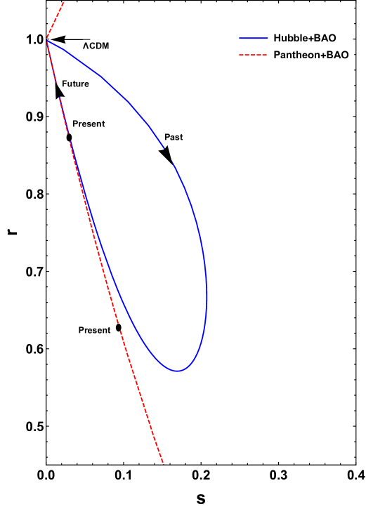
Figure 13: The evolution trajectories of the given model in $s-r$ plane corresponding to the values of model parameters constrained by the Hubble and Pantheon datasets together with BAO datasets.

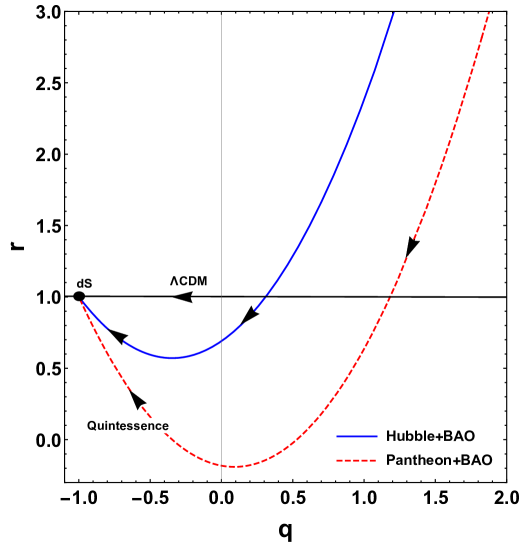
Figure 14: The evolution trajectories of the given model in $q-r$ plane corresponding to the values of model parameters constrained by the Hubble and Pantheon datasets together with BAO datasets.

The statefinder diagnostic can differentiate the variety of dark energy models like quintessence, the Chaplygin gas, braneworld models, etc. See the references [91, 92, 93]. The departure of our bulk viscous model from this fixed point establishes the distance of the given model from $\Lambda$CDM model. In present epoch the given model lie in Quintessence region $(s>0,r<1)$. We can observe that the trajectories of $s-r$ diagram will pass through the $\Lambda$CDM fixed point in the future. Thus the statefinder diagnostic successfully shows that the given model is different from other models of dark energy.

VIII Conclusions

In this article, we analyzed the evolution of FLRW universe dominated with non-relativistic bulk viscous matter, where the time-dependent bulk viscosity has the form $\xi=\xi_{0}+\xi_{1}H+\xi_{2}\left(\frac{\dot{H}}{H}+H\right)$. From the cosmic scale factor we found that in case of first limiting conditions the deceleration parameter shows the transition from deceleration to acceleration phase in past if  $\bar{\xi}_{0}+\bar{\xi}_{1}>\bar{\alpha}$, at present if $\bar{\xi}_{0}+\bar{\xi}_{1}=\bar{\alpha}$ and in the future if $\bar{\xi}_{0}+\bar{\xi}_{1}<\bar{\alpha}$. For second limiting conditions transition occur in the past if $\bar{\xi}_{0}+\bar{\xi}_{1}<\bar{\alpha}$, at present if $\bar{\xi}_{0}+\bar{\xi}_{1}=\bar{\alpha}$ and in the future if $\bar{\xi}_{0}+\bar{\xi}_{1}>\bar{\alpha}$. While in the absence of bulk viscosity i.e. $\xi_{0}=\xi_{1}=\xi_{2}=0$, the deceleration parameter becomes $q=\frac{1}{2}$. Hence, to describe the late-time acceleration of the expanding universe without invoking any dark energy component, the cosmic fluid with bulk viscosity is the most viable candidate. The second limiting condition is not suitable for present observational scenario, so we have considered the first limiting condition for our analysis. Further, for constraining the model and bulk viscous parameter we have used Hubble data and Pantheon data sets. Hence, from the Hubble datasets, we have the best fit ranges for the model parameters are $\alpha=-1.03_{-0.55}^{+0.52}$, $\xi_{0}=1.54_{-0.79}^{+0.83}$, $\xi_{1}=0.08_{-0.49}^{+0.49}$ and $\xi_{2}=0.66_{-0.83}^{+0.82}$ and from the Pantheon datasets, we have $\alpha=-1.33_{-0.43}^{+0.45}$, $\xi_{0}=0.10_{-0.12}^{+0.21}$, $\xi_{1}=1.81_{-0.87}^{+0.91}$ and $\xi_{2}=2.08_{-0.96}^{+0.91}$. Furthermore, including the six data points of the BAO datasets with the Hubble datasets and combine the results of Hubble constrained values, we obtain the values of the model parameters as, $\alpha=-1.06_{-0.82}^{+0.34}$, $\xi_{0}=2.25_{-1.7}^{+0.37}$, $\xi_{1}=0.08_{-0.96}^{+1.1}$ and $\xi_{2}=0.7_{-1.1}^{+1.1}$. Similarly, including the six data points of the BAO datasets with the Pantheon datasets and combine the results of Pantheon constrained values, we obtain the values of the model parameters as, $\alpha=-1.65_{-0.25}^{+0.85}$, $\xi_{0}=0.86_{-1.1}^{+0.29}$, $\xi_{1}=1.90_{-0.99}^{+0.97}$ and $\xi_{2}=1.93_{-0.91}^{+1.2}$. For the above set of values of the model parameters obtained are then used to plot the statefinder diagnostics. Finally, we conclude that the present bulk viscous model has been departed from $\Lambda$CDM point, in the present scenario it lie in quintessence region and it will again pass through the $\Lambda$CDM fixed point and hence our model is different from other models of the dark energy. We conclude that the bulk viscous theory can be considered as an alternate theory to describe the late time acceleration of the universe.

References

- [1] A.G. Riess et al., Astron. J. 116, 1009 (1998).
- [2] S. Perlmutter et al., Astrophys. J. 517, 565 (1999).
- [3] D.J. Eisenstein et al., Astrophys. J. 633, 560 (2005).
- [4] W.J. Percival at el., Mon. Not. R. Astron. Soc. 401, 2148 (2010).
- [5] C. Fedeli et al., Astron. Astrophy. 500, 667 (2009).
- [6] T. Koivisto, D.F. Mota, Phys. Rev. D 73, 083502 (2006).
- [7] S.F. Daniel, Phys. Rev. D 77, 103513 (2008).
- [8] R.R. Caldwell, M. Doran, Phys. Rev. D 69, 103517 (2004).
- [9] Z.Y. Huang et al., JCAP 0605, 013 (2006).
- [10] S. Weinberg, Rev. Mod. Phys. 61, 1 (1989).
- [11] S. M. Carroll et al., Annu. Rev. Astron. Astrophys. 30, 499 (1992).
- [12] E. J. Copeland et al., Int. J. Mod. Phys. D 15, 1753 (2006).
- [13] S. M. Carroll, Phys. Rev. Lett. 81, 3067 (1998).
- [14] Y. Fujii, Phys. Rev. D 26, 2580 (1982).
- [15] T. Chiba et al., Phys. Rev. D 62, 023511 (2000).
- [16] C. Armendariz-Picon et al., Phys. Rev. Lett. 85, 4438 (2000).
- [17] M. C. Bento et al., Phys. Rev. D 66, 043507 (2002).
- [18] A. Y. Kamenshchik et al., Phys. Lett. B 511, 265 (2001).
- [19] Hans A. Buchdahl, Mon. Not. Roy. Astron. Soc. 150, 1 (1970).
- [20] A. A. Starobinsky, Pisma Zh. Eksp. Teor. Fiz. 30, 719-723 (1979).
- [21] S. Nojiri, S.D. Odintsov, Phys. Rev. D 68, 123512 (2003).
- [22] R. Ferraro, F. Fiorini, Phys. Rev. D 75, 084031 (2007).
- [23] E. V. Linder, Phys. Rev. D 81, 127301 (2010).
- [24] K. Bamba et al., J. Cosmol. Astropart. Phys. 01, 021 (2011).
- [25] Sebastian Bahamonde et al., Eur. Phys. J. C 77, 2 (2017).
- [26] T. Harko et al., Phys. Rev. D 84, 024020 (2011).
- [27] Hamid Shabani, Mehrdad Farhoudi, Phys. Rev. D 88, 044048 (2013).
- [28] Yixin Xu et al., Eur. Phys. J. C 79, 708 (2019).
- [29] Simran Arora et al., Phys. Dark Univ. 30, 100664 (2020).
- [30] S. Nojiri et al., Prog. Theor. Phys. Suppl. 172, 81 (2008).
- [31] E. Elizalde et al., Class. Quant. Grav. 27, 095007 (2010).
- [32] K. Bamba et al., Eur. Phys. J. C 67, 295-310 (2010).
- [33] J. B. Jiménez et al., Phys. Rev. D 98, 044048 (2018).
- [34] T. Harko et al., Phys. Rev. D 98, 084043 (2018).
- [35] Sanjay Mandal et al., Phys. Rev. D 102, 024057 (2020).
- [36] Sanjay Mandal, Deng Wang and P.K. Sahoo, Phys. Rev. D 102, 124029 (2020).
- [37] Noemi Frusciante, Phys. Rev. D 103, 044021 (2021).
- [38] T. Padmanabhan, S. M. Chitre, Phys. Lett. A 120, 443 (1987).
- [39] I. Wega et al., Phys. Rev. D 33, 1839 (1986).
- [40] Athira Sasidharan, Titus K. Mathew, Eur. Phys. J. C 75, 348 (2015).
- [41] N D Jerin Mohan et al., Eur. Phys. J. C 77, 849 (2017).
- [42] Simran Arora et al., Class. Quant. Grav. 37, 205022 (2020).
- [43] G. C. Samanta, R. Myrzakulov, Chinese Journal of Physics 55, 1044-1054 (2017).
- [44] J. C. Fabris et al., Gen. Relativ. Gravit. 38, 495 (2006).
- [45] A. Avelino, U. Nucamendi, JCAP 04, 006 (2009).
- [46] W. Zindahl et al., Phys. Rev. D 64, 063501 (2001).
- [47] J. R. Wilson et al., Phys. Rev. D 75, 043521 (2007).
- [48] H. Okumura, F. Yonezawa, Physica A 321, 207-19 (2003).
- [49] C. Eckart, Phys. Rev. 58, 919(1940).
- [50] L. D. Landau, E. M. Lifshitz, Fluid Mechanics (Addison-Wesley, USA) (1959).
- [51] W. Israel, J. M. Stewart, Phys. Lett. B 58, 213 (1976).
- [52] W. Israel, Ann. Phys. (N.Y.) 100, 310 (1976).
- [53] W. Israel, J. M. Stewart, Proc. R. Soc. Lond. B 365, 43 (1979).
- [54] W. A. Hiscock, L. Lindblom, Phys. Rev. 31, 725 (1985).
- [55] W. A. Hiscock, J. Salmonson, Phys. Rev. D 43, 3249 (1991).
- [56] M. Cataldo et al., Phys. Lett. B 619, 005 (2005).
- [57] A. Avelino, U. Nucamendi, JCAP 8, 009 (2010).
- [58] S. D. Odintsov et al., Phys. Rev. D 101, 044010 (2020).
- [59] C. P. Singh, Pankaj Kumar, Eur. Phys. J. C 74, 3070 (2014).
- [60] S. Davood Sadatian, EPL 126, 30004 (2019).
- [61] G. J. Olmo and D. Rubiera-Garcia, Phys. Lett. B 740, 73 (2015).
- [62] J. Ren, X. H. Meng, Phys. Lett. B 633, 1 (2006).
- [63] D. Stern et al., J. Cosmol. Astropart. Phys. 02, 008(2010).
- [64] J. Simon et al., Phys. Rev. D 71, 123001(2005).
- [65] M. Moresco et al., J. Cosmol. Astropart. Phys. 08, 006(2012).
- [66] C. Zhang et al., Research in Astron. and Astrop. 14, 1221(2014).
- [67] M. Moresco et al., J. Cosmol. Astropart. Phys. 05, 014(2016).
- [68] A. L. Ratsimbazafy et al., Mon. Not. Roy. Astron. Soc. 467, 3239(2017).
- [69] M. Moresco, Mon. Not. Roy. Astron. Soc. Lett. 450, L16(2015).
- [70] E. Gaztaaga et al., Mon. Not. Roy. Astron. Soc. 399, 1663(2009).
- [71] A. Oka et al., Mon. Not. Roy. Astron. Soc. 439, 2515(2014).
- [72] Y. Wang et al., Mon. Not. Roy. Astron. Soc. 469, 3762(2017).
- [73] C. H. Chuang, Y. Wang, Mon. Not. Roy. Astron. Soc. 435, 255(2013).
- [74] S. Alam et al., Mon. Not. Roy. Astron. Soc. 470, 2617(2017).
- [75] C. Blake et al., Mon. Not. Roy. Astron. Soc. 425, 405(2012).
- [76] C. H. Chuang et al., Mon. Not. Roy. Astron. Soc. 433, 3559(2013).
- [77] L. Anderson et al., Mon. Not. roy. Astron. Soc. 441, 24(2014).
- [78] N. G. Busca et al., Astron. Astrophys. 552, A96(2013).
- [79] J. E. Bautista et al., Astron. Astrophys. 603, A12(2017).
- [80] T. Delubac et al., Astron. Astrophys. 574, A59(2015).
- [81] A. Font-Ribera et al., J. Cosmol. Astropart. Phys. 05, 027(2014).
- [82] G. S. Sharov, V. O. Vasiliev, Mathematical Modelling and Geometry 6, 1 (2018).
- [83] D. M. Scolnic et al., Astrophys. J. 859, 101(2018).
- [84] C. Blake et al., Mon. Not. Roy. Astron. Soc. 418, 1707 (2011).
- [85] W. J. Percival et al., Mon. Not. Roy. Astron. Soc. 401, 2148 (2010).
- [86] F. Beutler et al., Mon. Not. Roy. Astron. Soc. 416, 3017 (2011).
- [87] N. Jarosik et al., Astrophys. J. Suppl. 192, 14 (2011).
- [88] D. J. Eisenstein et al., Astrophys. J. 633, 560 (2005).
- [89] R. Giostri et al., J. Cosm. Astropart. Phys. 1203, 027 (2012).
- [90] V. Sahni et al., JETP Lett. 77, 201-206 (2003).
- [91] U. Alam et al., Mon. Not. R. Astron. Soc. 344, 1057(2003).
- [92] V. Gorini et al., Phys. Rev. D 67, 063509(2003).
- [93] W. Zimdahl and D. Pavon, Gen. Relativ. Gravit. 36, 1483(2004).