BAYESIAN TESTS OF SYMMETRY FOR

THE GENERALIZED VON MISES DISTRIBUTION

Sara Salvador (1) and Riccardo Gatto (2)

Submitted: July 2, 2020

Revised: April, 26 2021

Abstract

Bayesian tests on the symmetry of the generalized von Mises model for planar directions (Gatto and Jammalamadaka, , 2007) are introduced. The generalized von Mises distribution is a flexible model that can be axially symmetric or asymmetric, unimodal or bimodal. A characterization of axial symmetry is provided and taken as null hypothesis for one of the proposed Bayesian tests. The Bayesian tests are obtained by the technique of probability perturbation. The prior probability measure is perturbed so to give a positive prior probability to the null hypothesis, which would be null otherwise. This allows for the derivation of simple computational formulae for the Bayes factors. Numerical results reveal that, whenever the simulation scheme of the samples supports the null hypothesis, the null posterior probabilities appear systematically larger than their prior counterpart.

Key words and phrases

Axial symmetry; Bayes factor; circular distribution; probability perturbation; uni- and bimodality.

The authors are grateful to two anonymous Referees and an Associate Editor for several suggestions and corrections.

2010 Mathematics Subject Classification
            62H11 Directional data; spatial statistics
            62F15 Bayesian inference
            62F03 Hypothesis testing

Address
            Institute of Mathematical Statistics and Actuarial Science
            Department of Mathematics and Statistics
            University of Bern
            Alpeneggstrasse 22, 3012 Bern, Switzerland
            (1) sara.salvador@stat.unibe.ch, orcid.org/0000-0001-6492-645X
            (2) gatto@stat.unibe.ch, orcid.org/0000-0001-8374-6964

1 Introduction

In various scientific fields measurements can take the form of directions: the direction flight of a bird and the direction of earth’s magnetic pole are two examples. These directions can be in the plane, namely in two dimensions, as in the first example, or they can be in the space, namely in three dimensions, as in the second example. These measurements are called directional data and they appear in various scientific fields: in the analysis of protein structure, in machine learning, in forestry, in ornithology, in palaeomagnetism, in oceanography, in meteorology, in astronomy, etc. A two-dimensional direction is a point in $\mathbb{R}^{2}$ without magnitude, e.g. a unit vector. It can also be represented as a point on the circumference of the unit circle or as an angle, measured for example in radians and after fixing the null direction and the sense of rotation (clockwise or counter-clockwise). Because of this circular representation, observations on two-dimensional directional data are distinctively called circular data. During the last two or three decades, there has been a raise of interest for statistical methods for directional data. Recent applications can be found e.g. in Ley and Verdebout, (2018). Some monographs on this topic are Mardia and Jupp, (2000), Jammalamadaka and SenGupta, (2001), Ley and Verdebout, (2017) and also Pewsey et al., (2013). For a review article, see e.g. Gatto and Jammalamadaka, (2014).

The popular probability distribution for circular data, or circular distribution, is the circular normal or von Mises distribution, whose density is given in (3) below. This distribution is circularly symmetric around its unique mode. Until a couple decades ago, very few asymmetric circular distributions were available, two of these can be found in Sections 15.6 and 15.7 of Batschelet, (1981). In recent years, various asymmetric and multimodal circular distributions have been introduced, for example: Umbach and Jammalamadaka, (2009), Kato and Jones, (2015), Abe et al., (2013), Gatto and Jammalamadaka, (2003) and the generalized von Mises (GvM) of Gatto and Jammalamadaka, (2007). This article proposes three Bayesian tests for the GvM distribution. This distribution has density given

$$f(\theta\mid\mu_{1},\mu_{2},\kappa_{1},\kappa_{2}) =\frac{1}{2\pi G_{0}(\delta,\kappa_{1},\kappa_{2})}\exp\{\kappa_{1}\cos(\theta-\mu_{1})+\kappa_{2}\cos 2(\theta-\mu_{2})\},$$ (1)

$\forall\theta\in[0,2\pi)$, for given $\mu_{1}\in[0,2\pi)$, $\mu_{2}\in[0,\pi)$, $\delta=(\mu_{1}-\mu_{2})\mbox{\rm mod}\,\pi$, $\kappa_{1},\kappa_{2}>0$, and where the normalizing constant is given by

$$G_{0}(\delta,\kappa_{1},\kappa_{2}) =\frac{1}{2\pi}\int_{0}^{2\pi}\exp\{\kappa_{1}\cos\theta+\kappa_{2}\cos 2(\theta+\delta)\}d\theta.$$ (2)

We denote any circular random variable with this distribution by GvM($\mu_{1},\mu_{2},\kappa_{1},\kappa_{2}$). The well-known von Mises (vM) density is obtained by setting $\kappa_{2}=0$ in (1), giving

$$f(\theta\mid\mu,\kappa) =\frac{1}{2\pi I_{0}(\kappa)}\exp\{\kappa\cos(\theta-\mu)\},$$ (3)

$\forall\theta\in[0,2\pi)$, for given $\mu\in[0,2\pi)$, $\kappa>0$ and where $I_{\nu}(z)=(2\pi)^{-1}\int_{0}^{2\pi}\cos\nu\theta\,\exp\{z\cos\theta\}d\theta$, $z\in\mathbb{C}$, is the modified Bessel function $I$ of order $\nu$, with $\Re\nu>-1/2$, cf. 9.6.18 at p. 376 of Abramowitz and Stegun, (1972). We denote any circular random variable $\theta$ with this distribution by vM($\mu,\kappa$).

Besides its greater flexibility in terms of asymmetry and bimodality, the GvM distribution possesses the following properties that other asymmetric or multimodal circular distributions do not have.

1. After a re-parametrization, the GvM distribution belongs to the canonical exponential class. In this form, it admits a minimal sufficient and complete statistic; cf. Section 2.1 of Gatto and Jammalamadaka, (2007).

2. The maximum likelihood estimator and the trigonometric method of moments estimator of the parameters are the same; cf. Section 2.1 of Gatto, (2008). In this context, we should note that the computation of the maximum likelihood estimator is simpler with the GvM distribution than with the mixture of two vM distributions, as explained some lines below.

3. It is shown in Section 2.2 of Gatto and Jammalamadaka, (2007) that for fixed trigonometric moments of orders one and two, the GvM distribution is the one with largest entropy. The entropy gives a principle for selecting a distribution on the basis of partial knowledge: one should always choose distributions having maximal entropy, within distributions satisfying the partial knowledge. In Bayesian statistics, whenever a prior distribution has to be selected and information on the first two trigonometric moments is available, then the GvM is the optimal prior. For other theoretic properties of the GvM, see Gatto, (2009).

The mixture of two vM distributions is perhaps a more popular bimodal or asymmetric model then the GvM. However, the mixture does not share the given properties 1-3 of the GvM. The mixture is not necessarily more practical. While the likelihood of the GvM distribution is bounded, the likelihood of the mixture of the vM($\mu_{1},\kappa_{1}$) and the vM($\mu_{2},\kappa_{2}$) distributions is unbounded. As $\kappa_{1}\rightarrow\infty$, the likelihood when $\mu_{1}$ is equal to any one of the sample values tends to infinity. This follows from $I_{0}(\kappa_{1})\sim(2\pi\kappa_{1})^{-1/2}{\rm e}^{\kappa_{1}}$, as $\kappa_{1}\rightarrow\infty$; cf. Abramowitz and Stegun, (1972), 9.7.1 at p. 377. For alternative estimators to the maximum likelihood for vM mixtures, refer to Spurr and Koutbeiy, (1991).

Some recent applications of the GvM distributions are: Zhang et al., (2018), in meteorology, Lin and Dong, (2019), in oceanography, Astfalck et al., (2018), in offshore engineering, Christmas, (2014), in signal processing, and Gatto, (2021) in time series analysis.

The symmetry of a circular distribution is a fundamental question and, as previously mentioned, this topic has been studied in recent years. In the context of testing symmetry, one can mention: Pewsey, (2002), who proposes a test of symmetry around an unknown axis based on the second sine sample moment, and Pewsey, (2004), who considers the case where the symmetry is around the median axis. Both tests are frequentist and no Bayesian test of symmetry appears available in the literature. In fact, Bayesian analysis for circular data has remained underdeveloped, partly because of the lack of nice conjugate classes of distributions. Moreover, Bayesian analysis has focused on the vM model, which is symmetric. We refer to p. 278-279 of Jammalamadaka and SenGupta, (2001) for a review on Bayesian analysis for circular data.

In this context, this article proposes Bayesian tests of symmetry for the GvM model (1). The first test proposed concerns the parameter $\delta$. The null hypothesis is $\delta=0$, that is, no shift between cosines of frequency one and two. In this case, the distribution is symmetric around the axis passing through $\mu_{1}$. It is bimodal with one mode at $\mu_{1}$ and the other one at $\mu_{1}+\pi$, whenever $\kappa_{1}<4\kappa_{2}$. If $\kappa_{1}\geq 4\kappa_{2}$, then it is unimodal with mode at $\mu_{1}$. We refer to Table 1 of Gatto and Jammalamadaka, (2007). The second test is on the precise characterization of axial symmetry, i.e. on $\delta=0$ or $\delta=\pi/2$. So far $\kappa_{2}>0$ is considered and the third test is for $\kappa_{2}=0$, so that the distribution is no longer GvM but vM, which is is axially symmetric. The Bayesian tests rely on the method of probability perturbation, where the probability distribution of the null hypothesis is slightly perturbed, in order to give a positive prior probability to the null hypothesis, which would be null otherwise. It would be interesting to consider the above null hypotheses under the frequentist perspective, perhaps with the likelihood ratio approach. This topic is not studied in this article, in order to limit its length.

The remaining part of this article is organized as follows. Section 2 gives the derivation of these Bayesian tests and their Bayes factors. Section 2.1 presents the approach used for these tests: Section 2.2 considers the test of no shift between cosines, Section 2.3 considers the test of symmetry and Section 2.4 considers the test of vM axial symmetry. Numerical results are presented in Section 3: Section 3.1 presents a Monte Carlo study of the the tests of Section 2.1 whereas Section 3.2 presents the application to some real data. Final remarks are given in Section 4.

2 Bayesian tests and perturbation method for the GvM model

The proposed tests rely on Bayes factors. The Bayes factor $B_{01}$ indicates the evidence of the null hypothesis with respect to (w.r.t.) the general alternative. Let us denote by $\bm{\theta}=(\theta_{1},\ldots,\theta_{n})$ the sample. Then

$$B_{01}=\frac{P[\bm{\theta}|{\mbox{H}}_{0}]}{P[\bm{\theta}|{\mbox{H}}_{1}]}=\frac{P[{\mbox{H}}_{0}|\bm{\theta}]}{P[{\mbox{H}}_{1}|\bm{\theta}]}\cdot\frac{P[{\mbox{H}}_{1}]}{P[{\mbox{H}}_{0}]}=\frac{R_{1}}{R_{0}},$$ (4)

where

$$R_{0}=\frac{P[{\mbox{H}}_{0}]}{P[{\mbox{H}}_{1}]}=\frac{P[{\mbox{H}}_{0}]}{1-P[{\mbox{H}}_{0}]}\leavevmode\nobreak\ \leavevmode\nobreak\ \text{and}\leavevmode\nobreak\ \leavevmode\nobreak\ R_{1}=\frac{P[{\mbox{H}}_{0}|\bm{\theta}]}{P[{\mbox{H}}_{1}|\bm{\theta}]}=\frac{P[{\mbox{H}}_{0}|\bm{\theta}]}{1-P[{\mbox{H}}_{0}|\bm{\theta}]},$$

are the prior and the posterior odds, respectively. The case $B_{01}>1$ indicates evidence for ${\mbox{H}}_{0}$. Interpretations of the values of the Bayes factor can be found in Jeffreys, (1961) and Kass and Raftery, (1995). Our synthesis of these interpretations is given in Table 1, which provides a qualitative scale for the Bayes factor.

$B_{01}$	evidence for ${\mbox{H}}_{0}$
$<1$	negative
1 to 1.5	not worth more than a bare mention
1.5 to 5	positive
5 to 10	substantial
10 to 20	strong
$>20$	decisive

Table 1: Guidelines for the interpretation of Bayes factors.

The null hypotheses of this article are simple, in the sense that they concern only points of the parametric space. The fact that these points have probability null does not allow for the computation of Bayes factors. Therefore we use an approach with probability perturbation explained in the next section.

2.1 Bayesian tests of simple hypotheses

The practical relevance of a simple null hypothesis, i.e. of the type ${\mbox{H}}_{0}:\xi=\xi_{0}$, has been widely debated in the statistical literature. According to Berger and Delampady, : “it is rare, and perhaps impossible, to have a null hypothesis that can be exactly modelled as $\theta=\theta_{0}$”. They illustrate their claim by the following example. “More common precise hypotheses such as ${\mbox{H}}_{0}$:Vitamin C has no effect on the common cold are clearly not meant to be though of as exact point nulls; surely vitamin C has some effects, although perhaps a very miniscule effect.” A similar example involving forensic science can be found in Lindley, (1977). When the parameter $\xi$ is of continuous nature, it is usually more realistic to consider null hypotheses of the type ${\mbox{H}}_{0,\varepsilon}:|\xi-\xi_{0}|\leq\varepsilon/2$, for some small $\varepsilon>0$. This solves also the problem of the vanishing prior probability of ${\mbox{H}}_{0}$, namely $P[\xi=\xi_{0}]=0$. This problem is sometimes addressed by giving a positive probability to $\{\xi=\xi_{0}\}$. However, Berger and Sellke, (1987) explain that the two approaches should be related. “It is convenient to specify a prior distribution for the testing problem as follows: let $0<\pi_{0}<1$ denote the prior probability of ${\mbox{H}}_{0}:\theta=\theta_{0}$ … One might question the assignment of a positive probability to ${\mbox{H}}_{0}$, because it is rarely the case that it is thought possible for $\theta=\theta_{0}$ to hold exactly … ${\mbox{H}}_{0}$ is to be understood as simply an approximation to the realistic hypothesis ${\mbox{H}}_{0}:|\theta-\theta_{0}|\leq b$ and $\pi_{0}$ is to be interpreted as the prior probability that would be assigned to $\{\theta:|\theta-\theta_{0}|\leq b\}$.” Accordingly, we assign to the original simple hypothesis ${\mbox{H}}_{0}:\xi=\xi_{0}$ the prior probability $p_{0}>0$ of ${\mbox{H}}_{0,\varepsilon}:\xi\in[\xi_{0}-\varepsilon/2,\xi_{0}+\varepsilon/2]$, for some $\varepsilon>0$. Thus, we replace the prior probability measure $P$ by its perturbation, obtained by the assignment of the probability $p_{0}>0$ to $\{\xi_{0}\}$. We denote by $P_{0}$ the probability measure $P$ with the $p_{0}$-perturbation. To summarize: the point null hypotheses is made relevant with $p_{0}=P_{0}[\xi=\xi_{0}]=P\left[\delta\in\left[\xi_{0}-\varepsilon/2,\xi_{0}+\varepsilon/2\right]\right]>0$.

The length $\varepsilon$ of the neighbourhood of $\xi_{0}$, which determines the prior probability $p_{0}$ of ${\mbox{H}}_{0}$ under the perturbed model, should not be too small. A significant value of $p_{0}$ for the null hypothesis is in fact coherent with the frequentist approach of hypotheses tests, where computations of rejection regions or P-values are carried over under the null hypothesis. Berger, (1985), p. 149, states that $\varepsilon$ has to be chosen such that any $\xi$ in $(\xi_{0}-\varepsilon/2,\xi_{0}+\varepsilon/2)$ becomes “indistinguishable” from $\xi_{0}$, while Berger and Sellke, state that $\varepsilon$ has to be “small enough” so that ${\mbox{H}}_{0,\varepsilon}$ can be “accurately approximated” by ${\mbox{H}}_{0}$. A related reference is Berger and Delampady, (1987), who studied this problem with a Gaussian model, and Berger, (1985), p. 149, who obtains an upper bound for the radius $\varepsilon/2$ under a simple Gaussian model. Two other references on the practical relevance of simple null hypotheses are Jeffreys, (1961) and Zellner, (1984).

We end this section with some comments regarding the choice of the prior distribution of $\xi$. This is a generally unsolved problem of Bayesian statistics and widely discussed in the literature, see e.g. Jeffreys, (1961) and Kass and Wasserman, (1996). According to Berger and Delampady, (1987), there is “no choice of the prior that can claim to be objective”. In this article we follow the directives given in Berger and Delampady, (1987) and Berger and Sellke, (1987), where various details on the choice of the prior are discussed and some classes of priors are analysed. According to Berger and Delampady, (1987), in absence of prior information, the prior should be symmetric about $\xi_{0}$ and non-increasing w.r.t. $|\xi-\xi_{0}|$. Otherwise, one could find some “favoured” alternative values of $\xi$; cf. Berger and Sellke, (1987). Our choices of priors are presented in Section 3: for each test of the study we compute Bayes factors under priors obtained by varying the concentration around the generic value $\xi_{0}$.

2.2 Test of no shift between cosines of GvM

Consider the Bayesian test on the GvM model (1) of the null the hypothesis

$$\text{H}_{0}:\delta=0,$$

where $\delta=(\mu_{1}-\mu_{2})\leavevmode\nobreak\ \text{mod}\leavevmode\nobreak\ \pi$ and where the values of $\mu_{1},\kappa_{1},\kappa_{2}$ are assumed known and equal to $\mu_{1}^{0},\kappa_{1}^{0},\kappa_{2}^{0}$, respectively. Under the original probability measure $P$, the random parameter $\delta$ has an absolutely continuous prior distribution and so $P[\delta=0]=0$. According to Section 2.1 we define the perturbation of the probability measure $P$, denoted $P_{0}$, for which $p_{0}=P_{0}[\delta=0]>0$. This perturbation is the assignment to $\{\delta=0\}$ of the probability mass that initially lies close to that $P$-null set. Let $\varepsilon>0$ and consider the set

$$\mathcal{A}_{\varepsilon} =\left\{\delta\in[0,\pi)\Big{|}\delta\in\left[0,\frac{\varepsilon}{2}\right]\cup\left[\pi-\frac{\varepsilon}{2},\pi\right)\right\}.$$ (5)

The complement is

$$\mathcal{A}^{{\sf c}}_{\varepsilon} =\left\{\delta\in[0,\pi)\Big{|}\delta\in\left(\frac{\varepsilon}{2},\pi-\frac{\varepsilon}{2}\right)\right\}.$$

Note that (5) refers to a neighbourhood of the origin of the circle of circumference $\pi$. We thus assign to $p_{0}$ the value

$$p_{0} =P\left[\mathcal{A}_{\varepsilon}\right],$$ (6)

for some suitably small $\varepsilon>0$. The prior distribution function (d.f.) under the perturbed probability measure $P_{0}$ at any $\delta\in[0,\pi)$ is given by

$$p_{0}\Delta(\delta^{\prime})+(1-p_{0})G(\delta^{\prime}).$$ (7)

where $G$ denotes the prior d.f. of $\delta$ and where $\Delta$ is the Dirac d.f., which assigns mass one to the origin. Denote by $g$ the density of $G$. If $0\notin(\delta^{\prime},\delta^{\prime}+d\delta^{\prime})$, for some $\delta^{\prime}\in(0,\pi)$, where the relations $\in$ and $\notin$ are meant circularly over the circle of circumference $\pi$, then (7) implies

$$\begin{split}P_{0}[\delta\in(\delta^{\prime},\delta^{\prime}+d\delta^{\prime})]&=(1-p_{0})g(\delta^{\prime})d\delta^{\prime}=(1-p_{0})P[\delta\in(\delta^{\prime},\delta^{\prime}+d\delta^{\prime})].\end{split}$$ (8)

Let $\theta_{1},\ldots,\theta_{n}$ be independent circular random variables that follow the GvM distribution (1). For simplicity, we denote the joint density of $\bm{\theta}=(\theta_{1},\ldots,\theta_{n})$, with the fixed values $\delta^{\prime}$, $\mu_{1}^{0}$, $\kappa_{1}^{0}$ and $\kappa_{2}^{0}$, as

$$f(\bm{\theta}|\delta^{\prime}) =\left\{2\pi G_{0}(\delta^{\prime},\kappa_{1}^{0},\kappa_{2}^{0})\right\}^{-n}\exp\left\{\kappa_{1}^{0}\sum_{i=1}^{n}\cos(\theta_{i}-\mu_{1}^{0})+\kappa_{2}^{0}\sum_{i=1}^{n}\cos 2(\theta_{i}-\mu_{1}^{0}+\delta^{\prime})\right\}.$$ (9)

When considered as a function of $\delta^{\prime}$, (9) becomes the likelihood of $\delta$. Then, by (8) the marginal density of $\bm{\theta}=(\theta_{1},\ldots,\theta_{n})$ under the perturbed probability is given by

$$m(\bm{\theta}) =\int_{[0,\pi)}f(\bm{\theta}|\delta^{\prime})P_{0}[\delta\in(\delta^{\prime},\delta^{\prime}+d\delta^{\prime})]$$

$$=\int_{\mathcal{A}_{\varepsilon}}f(\bm{\theta}|\delta^{\prime})P_{0}[\delta\in(\delta^{\prime},\delta^{\prime}+d\delta^{\prime})]+(1-p_{0})\int_{\mathcal{A}_{\varepsilon}^{\mathsf{c}}}f(\bm{\theta}|\delta^{\prime})g(\delta^{\prime})d\delta^{\prime}$$

$$=p_{0}f(\bm{\theta}|0)+(1-p_{0})\int_{\mathcal{A}_{\varepsilon}}f(\bm{\theta}|\delta^{\prime})g(\delta^{\prime})d\delta^{\prime}+(1-p_{0})\int_{\mathcal{A}_{\varepsilon}^{\mathsf{c}}}f(\bm{\theta}|\delta^{\prime})g(\delta^{\prime})d\delta^{\prime}$$

$$\sim 2p_{0}f(\bm{\theta}|0)+(1-p_{0})\int_{\mathcal{A}_{\varepsilon}^{\mathsf{c}}}f(\bm{\theta}|\delta^{\prime})g(\delta^{\prime})d\delta^{\prime},\leavevmode\nobreak\ \text{as $\varepsilon\rightarrow 0$}.$$ (10)

The above asymptotic equivalence is due to

$$(1-p_{0})\int_{\mathcal{A}_{\varepsilon}}f(\bm{\theta}|\delta^{\prime})g(\delta^{\prime})d\delta^{\prime} =(1-p_{0})p_{0}\int_{\mathcal{A}_{\varepsilon}}f(\bm{\theta}|\delta^{\prime})\frac{g(\delta^{\prime})}{p_{0}}d\delta^{\prime}\sim p_{0}f(\theta|0),\;\text{as $\varepsilon\rightarrow 0$}.$$

The posterior perturbed probability, namely the conditional perturbed probability of $\{\delta=0\}$ given $\bm{\theta}$, can be approximated as follows,

$$\begin{split}P_{0}[\delta=0|\bm{\theta}]&\sim\frac{p_{0}f(\bm{\theta}|0)}{2p_{0}f(\bm{\theta}|0)+(1-p_{0})\int_{\mathcal{A}_{\varepsilon}^{\mathsf{c}}}f(\bm{\theta}|\delta^{\prime})g(\delta^{\prime})d\delta^{\prime}}\\ &=\frac{1}{2}\Bigg{(}1+\frac{1-p_{0}}{p_{0}}\frac{\int_{\mathcal{A}_{\varepsilon}^{\mathsf{c}}}f(\bm{\theta}|\delta^{\prime})g(\delta^{\prime})d\delta^{\prime}}{2f(\bm{\theta}|0)}\Bigg{)}^{-1},\;\text{ as }\varepsilon\rightarrow 0.\end{split}$$ (11)

In order to compute the Bayes factor for this test, we define the prior odds $R_{0}=p_{0}/(1-p_{0})$ and the posterior odds $R_{1}=P_{0}[\delta=0|\bm{\theta}]/(1-P_{0}[\delta=0|\bm{\theta}])$. The Bayes factor is the posterior over the prior odds, namely $B_{01}=R_{1}/R_{0}$. Clearly $p_{0}\leq P_{0}[\delta=0|\bm{\theta}]$ iff $B_{01}\geq 1$ and, the larger $P_{0}[\delta=0|\bm{\theta}]-p_{0}$ becomes, the larger $B_{01}$ becomes: a large Bayes factor tells that the data support the null hypothesis. From the approximation

$$\begin{split}R_{1}&\sim\left[1+\frac{1-p_{0}}{p_{0}}\frac{\int_{\mathcal{A}_{\varepsilon}^{\mathsf{c}}}f(\bm{\theta}|\delta^{\prime})g(\delta^{\prime})d\delta^{\prime}}{f\left(\bm{\theta}|0\right)}\right]^{-1}\end{split}$$

and from some simple algebraic manipulation, we obtain the computable approximation to the Bayes factor $B_{01}=R_{1}/R_{0}$ given by

$$B_{01}\sim\frac{f(\bm{\theta}|0)}{\int_{\mathcal{A}_{\varepsilon}^{\mathsf{c}}}f(\bm{\theta}|\delta^{\prime})g(\delta^{\prime})d\delta^{\prime}},\leavevmode\nobreak\ \text{as $\varepsilon\rightarrow 0$}.$$ (12)

The representation of the Bayes factor (12) is asymptotically correct and we remind that, in the context where we approximate the null hypothesis with a neighbourhood by the point null hypothesis, the reasoning is always of asymptotic nature. A reference for this perturbation technique is Berger, (1985), p. 148-150.

Regarding the large sample asymptotics of the proposed test, it is know that, for a sample of $n$ independent random variables with common distribution with true parameter $\xi_{0}$, the posterior distribution converges to the distribution with total mass over $\xi_{0}$, as $n\to\infty$. This means that the posterior mode is a consistent estimator. We deduce that, under ${\mbox{H}}_{0}$,

$$P_{0}[\delta=0|\bm{\theta}] =P[{\cal A}_{\varepsilon}|\bm{\theta}]\stackrel{{\scriptstyle P}}{{\longrightarrow}}1,\;\text{ as }n\to\infty.$$

Consequently, $R_{1}=P_{0}[\delta=0|\bm{\theta}]/(1-P_{0}[\delta=0|\bm{\theta}])\stackrel{{\scriptstyle P}}{{\longrightarrow}}\infty$ and $B_{01}=R_{1}/R_{0}\stackrel{{\scriptstyle P}}{{\longrightarrow}}\infty$, as $n\to\infty$. The Bayesian test of ${\mbox{H}}_{0}:\delta=0$ is consistent in this sense.

We now give some computational remarks that are also valid for the tests of Sections 2.3 and 2.4. The integral appearing in the denominator of (12) can be easily evaluated by Monte Carlo integration. For a given large integer $s$, we generate $\delta^{{(i)}}$, for $i=1,\ldots,s$, from the density $g$ and then we compute the approximation

$$\int_{\mathcal{A}_{\varepsilon}^{\mathsf{c}}}f(\bm{\theta}|\delta^{\prime})g(\delta^{\prime})d\delta^{\prime} =\int_{\mathcal{A}_{\varepsilon}^{\mathsf{c}}}f(\bm{\theta}|\delta^{\prime})P[\delta\in(\delta^{\prime},\delta^{\prime}+d\delta^{\prime})]\simeq\frac{1}{s}\sum_{i=1}^{s}f(\bm{\theta}|\delta^{(i)})\text{I}\{\delta^{(i)}\in\mathcal{A}_{\varepsilon}^{\mathsf{c}}\},$$ (13)

where $\text{I}\{A\}$ denotes the indicator of statement or event $A$. For the computation normalizing constant of the GvM distribution given in (2) one can use the Fourier series

$$G_{0}(\delta,\kappa_{1},\kappa_{2})=I_{0}(\kappa_{1})I_{0}(\kappa_{2})+2\sum_{j=1}^{\infty}I_{2j}(\kappa_{1})I_{j}(\kappa_{2})\cos 2j\delta,$$ (14)

where $\delta\in[0,\pi)$ and $\kappa_{1},\kappa_{2}>0$, see e.g. Gatto and Jammalamadaka, (2007).

2.3 Test of axial symmetry of GvM

In this section we consider the Bayesian test of axial symmetry for the GvM model (1). A circular density $g$ is symmetric around the angle $\alpha/2$, for some $\alpha\in[0,2\pi)$, if $g(\theta)=g(\alpha-\theta)$, $\forall\theta\in[0,2\pi)$. In this case we have also $g(\theta)=g((\alpha+2\pi)-\theta)$, so that symmetry around $\alpha/2+\pi$ holds as well: the symmetry is indeed an axial one.

Proposition 2.1 (Characterization of axial symmetry for the GvM distribution).

The GvM distribution (1) is axial symmetric iff

$$\delta=0\;\text{ or }\;\delta=\frac{\pi}{2}.$$

In both cases, the axis of symmetry has angle $\mu_{1}$.

The proof of Proposition 2.1 is given in Appendix A.

Note that $\delta$ is defined modulo $\pi$ and that for $\kappa_{2}=0$ or $\kappa_{1}=0$ the GvM reduces respectively to the vM or to the axial vM, defined later as $\text{vM}_{2}$ and given in (18). These two distributions are clearly symmetric, but Proposition 2.1 gives the characterization of symmetry in terms of $\delta$ since we define the GvM distribution in (1) with concentration parameters $\kappa_{1},\kappa_{2}>0$.

As mentioned at the beginning of the section, symmetry of a circular distribution around an angle is the symmetry around an axis. For the GvM density, this is made explicit in (21), where adding $2\pi$ to $\alpha$ would not have any influence. Figure 1 provides two numerical illustrations of the axial symmetry of the GvM distribution. The graph in Figure 1a shows the density of the GvM($\pi,\pi,0.1,5.5$) distribution: $\delta=0$ and the axis of symmetry is at angle $\mu_{1}=\pi$. The graph in Figure 1b shows the density of the GvM($\pi/2,0,5.5,0.1$) distribution: $\delta=\pi/2$ and the axis of symmetry is at angle $\mu_{1}=\pi/2$.

(a) GvM($\pi,0,0.1,5.5$) density ($\delta=0$).

(b) GvM($\pi/2,0,5.5,0.1$) density ($\delta=\pi/2$).

Figure 1: Two axial symmetric GvM densities over the interval $(-2\pi,2\pi)$ and with their axis of symmetry at angle $\mu_{1}$ shown by vertical dashed lines.

Thus, Proposition 2.1 allows us to write the null hypothesis of axial symmetry as

$$\text{H}_{0}:\delta=0\text{ or }\delta=\frac{\pi}{2},$$

where the values of $\mu_{1},\kappa_{1},\kappa_{2}$ are assumed known and equal to $\mu_{1}^{0},\kappa_{1}^{0},\kappa_{2}^{0}$, respectively. The Bayesian test is obtained by perturbation of the probability measure $P$, which is denoted $P_{0}$. The probabilities

$$p_{0}=P_{0}[\delta=0]>0\;\text{ and }\;p_{\frac{\pi}{2}}=P_{0}\left[\delta=\frac{\pi}{2}\right]>0$$

are the probabilities masses of $\{\delta=0\}$ and $\{\delta=\frac{\pi}{2}\}$ of the perturbed measure, respectively. They are obtained from

$$p_{0}=P\left[\delta\in\left[0,\frac{\varepsilon}{2}\right]\cup\left[\pi-\frac{\varepsilon}{2},\pi\right)\right]\;\text{ and }p_{\frac{\pi}{2}}=P\left[\delta\in\left[\frac{\pi}{2}-\frac{\varepsilon}{2},\frac{\pi}{2}+\frac{\varepsilon}{2}\right]\right],$$

for suitably small $\varepsilon>0$. As is Section 2.2, the prior d.f. of $\delta$ under the perturbed probability $P_{0}$ at any $\delta^{\prime}\in[0,\pi)$ is given by

$$p_{0}\Delta(\delta^{\prime})+p_{\frac{\pi}{2}}\Delta\left(\delta^{\prime}-\frac{\pi}{2}\right)+\left\{1-\left(p_{0}+p_{\frac{\pi}{2}}\right)\right\}G(\delta^{\prime}),$$ (15)

where $G$ is the prior d.f. of $\delta$ under $P$. It follows from (15) that for $0,\pi/2\notin(\delta^{\prime},\delta^{\prime}+d\delta^{\prime})$, for some $\delta^{\prime}\in(0,\pi)\setminus\{\pi/2\}$,

$$P_{0}[\delta\in(\delta^{\prime},\delta^{\prime}+d\delta^{\prime})]=\left[1-\left(p_{0}+p_{\frac{\pi}{2}}\right)\right]g(\delta^{\prime})d\delta^{\prime}=\left[1-\left(p_{0}+p_{\frac{\pi}{2}}\right)\right]P[\delta\in(\delta^{\prime},\delta^{\prime}+d\delta^{\prime})],$$

where $g$ is the density of $G$.

Let

$$\mathcal{B}_{\varepsilon,0}=\left\{\delta\in[0,\pi)\Big{|}\delta\in\left[0,\frac{\varepsilon}{2}\right]\cup\left[\pi-\frac{\varepsilon}{2},\pi\right)\right\},\leavevmode\nobreak\ \text{ and }\mathcal{B}_{\varepsilon,\frac{\pi}{2}}=\left\{\delta\in[0,\pi)\Big{|}\delta\in\left[\frac{\pi}{2}-\frac{\varepsilon}{2},\frac{\pi}{2}+\frac{\varepsilon}{2}\right]\right\}.$$

Define

$$\mathcal{B}_{\varepsilon}=\left\{\delta\in[0,\pi)\Big{|}\delta\in\left[0,\frac{\varepsilon}{2}\right]\cup\left[\pi-\frac{\varepsilon}{2},\pi\right)\vee\delta\in\left[\frac{\pi}{2}-\frac{\varepsilon}{2},\frac{\pi}{2}+\frac{\varepsilon}{2}\right]\right\}=\mathcal{B}_{\varepsilon,0}\cup\mathcal{B}_{\varepsilon,\frac{\pi}{2}}.$$

Its complement is given by

$$\mathcal{B}_{\varepsilon}^{\mathsf{c}}=\left\{\delta\in[0,\pi)\Big{|}\delta\in\left(\frac{\varepsilon}{2},\frac{\pi}{2}-\frac{\varepsilon}{2}\right)\cup\left(\frac{\pi}{2}+\frac{\varepsilon}{2},\pi-\frac{\varepsilon}{2}\right)\right\}.$$

The marginal density of $\bm{\theta}=(\theta_{1},\ldots,\theta_{n})$ w.r.t. the perturbed probability $P_{0}$ is given by

$$\begin{split}m(\bm{\theta})&=\int_{[0,\pi)}f(\bm{\theta}|\delta^{\prime})P_{0}[\delta\in(\delta^{\prime},\delta^{\prime}+d\delta^{\prime})]\\ &=\int_{\mathcal{B}_{\varepsilon}}f(\bm{\theta}|\delta^{\prime})P_{0}[\delta\in(\delta^{\prime},\delta^{\prime}+d\delta^{\prime})]+\left[1-\left(p_{0}+p_{\frac{\pi}{2}}\right)\right]\int_{\mathcal{B}_{\varepsilon}^{\mathsf{c}}}f(\bm{\theta}|\delta^{\prime})g(\delta^{\prime})d\delta^{\prime}\\ &=p_{0}f(\bm{\theta}|0)+p_{\frac{\pi}{2}}f\left(\bm{\theta}|\frac{\pi}{2}\right)+\left[1-\left(p_{0}+p_{\frac{\pi}{2}}\right)\right]\int_{\mathcal{B}_{\varepsilon}}f(\bm{\theta}|\delta^{\prime})g(\delta^{\prime})d\delta^{\prime}\\ &\quad\qquad+\left[1-\left(p_{0}+p_{\frac{\pi}{2}}\right)\right]\int_{\mathcal{B}_{\varepsilon}^{\mathsf{c}}}f(\bm{\theta}|\delta^{\prime})g(\delta^{\prime})d\delta^{\prime}\\ &\sim 2p_{0}f(\bm{\theta}|0)+2p_{\frac{\pi}{2}}f\left(\bm{\theta}\Big{|}\frac{\pi}{2}\right)+\left[1-\left(p_{0}+p_{\frac{\pi}{2}}\right)\right]\int_{\mathcal{B}_{\varepsilon}^{\mathsf{c}}}f(\bm{\theta}|\delta^{\prime})g(\delta^{\prime})d\delta^{\prime},\leavevmode\nobreak\ \text{as $\varepsilon\rightarrow 0$}.\end{split}$$

In the asymptotic equivalence, as in Section 2.2, we notice that

$$\begin{split}&\left[1-\left(p_{0}+p_{\frac{\pi}{2}}\right)\right]\int_{\mathcal{B}_{\varepsilon}}f(\bm{\theta}|\delta^{\prime})g(\delta^{\prime})d\delta^{\prime}\\ &=\left[1-\left(p_{0}+p_{\frac{\pi}{2}}\right)\right]\left[\int_{\mathcal{B}_{\varepsilon,0}}f(\bm{\theta}|\delta^{\prime})g(\delta^{\prime})d\delta^{\prime}+\int_{\mathcal{B}_{\varepsilon,\frac{\pi}{2}}}f(\bm{\theta}|\delta^{\prime})g(\delta^{\prime})d\delta^{\prime}\right]\\ &=\left[1-\left(p_{0}+p_{\frac{\pi}{2}}\right)\right]\left[p_{0}\int_{\mathcal{B}_{\varepsilon,0}}f(\bm{\theta}|\delta^{\prime})\frac{g(\delta^{\prime})}{p_{0}}d\delta^{\prime}+p_{\frac{\pi}{2}}\int_{\mathcal{B}_{\varepsilon,\frac{\pi}{2}}}f(\bm{\theta}|\delta^{\prime})\frac{g(\delta^{\prime})}{p_{\frac{\pi}{2}}}d\delta^{\prime}\right]\\ &\sim p_{0}f(\bm{\theta}|0)+p_{\frac{\pi}{2}}f\left(\bm{\theta}\Big{|}\frac{\pi}{2}\right),\leavevmode\nobreak\ \text{ as }\varepsilon\rightarrow 0.\end{split}$$

The posterior probability of $\{\delta=0\vee\delta=\pi/2\}$ under the perturbed probability measure is given by

$$\begin{split}P_{0}\left[\delta=0\vee\delta=\frac{\pi}{2}\Big{|}\bm{\theta}\right]&\sim\frac{p_{0}f(\bm{\theta}\lvert 0)+p_{\frac{\pi}{2}}f(\bm{\theta}|\frac{\pi}{2})}{2p_{0}f(\bm{\theta}|0)+2p_{\frac{\pi}{2}}f(\bm{\theta}|\frac{\pi}{2})+[1-(p_{0}+p_{\frac{\pi}{2}})]\mathcal{I}_{1}(\theta)}\\ &=\frac{1}{2}\left[1+\frac{\left[1-(p_{0}+p_{\frac{\pi}{2}})\right]\mathcal{I}_{1}(\bm{\theta})}{2p_{0}f(\bm{\theta}|0)+2p_{\frac{\pi}{2}}f(\bm{\theta}|\frac{\pi}{2})}\right]^{-1},\;\text{ as }\varepsilon\to 0,\end{split}$$

where

$$\mathcal{I}_{1}(\bm{\theta})=\int_{\mathcal{B}_{\varepsilon}^{\mathsf{c}}}f(\bm{\theta}|\delta^{\prime})g(\delta^{\prime})d\delta^{\prime}.$$

With this we obtain the following approximation to the posterior odds,

$$\begin{split}R_{1}=\frac{P_{0}\left[\delta=0\vee\delta=\frac{\pi}{2}|\bm{\theta}\right]}{1-P_{0}\left[\delta=0\vee\delta=\frac{\pi}{2}|\bm{\theta}\right]}=\left[\frac{1}{P_{0}\left[\delta=0\vee\delta=\frac{\pi}{2}|\bm{\theta}\right]}-1\right]^{-1}\sim\left[1+\frac{\left[1-(p_{0}+p_{\frac{\pi}{2}})\right]\mathcal{I}_{1}}{p_{0}f(\bm{\theta}|0)+p_{\frac{\pi}{2}}f(\bm{\theta}\big{|}\frac{\pi}{2})}\right]^{-1}\end{split}$$

as $\varepsilon\rightarrow 0$. With the prior odds given by

$$R_{0}=\frac{p_{0}+p_{\frac{\pi}{2}}}{1-(p_{0}+p_{\frac{\pi}{2}})}$$

and after algebraic manipulations, we obtain the approximation to the Bayes factor given by

$$B_{01}\sim\frac{p_{0}f(\bm{\theta}|0)+p_{\frac{\pi}{2}}f(\bm{\theta}|\frac{\pi}{2})}{(p_{0}+p_{\frac{\pi}{2}})\mathcal{I}_{1}(\bm{\theta})},\leavevmode\nobreak\ \leavevmode\nobreak\ \text{as $\varepsilon\rightarrow 0$}.$$

2.4 Test of vM axial symmetry

We consider the Bayesian test of the null hypothesis that the sample follows a vM distribution against the alternative that it comes from an arbitrary GvM distribution. This null hypothesis implies axial symmetry in the class of vM distributions, whereas the alternative hypothesis includes both symmetric or asymmetric GvM distributions. Precisely, we have $\text{H}_{0}:\kappa_{2}=0$, where $\mu_{1},\mu_{2}$ and $\kappa_{1}$ are assumed known and equal to $\mu_{1}^{0},\mu_{2}^{0}$ and $\kappa_{1}^{0}$ respectively. The GvM with $\kappa_{2}=0$ reduces to the trivially symmetric vM distribution. Formally, the GvM is defined for $\kappa_{2}>0$ only, so that the symmetry considered here is no longer within the GvM class but it is rather a vM axial symmetry. This symmetry within the GvM class should be thought as approximate, for vanishing values of $\kappa_{2}$.

Symmetry with the GvM formula can also be obtained with $\kappa_{1}=0$, in which case the GvM formula reduces to an axial von Mises distribution $\text{vM}_{2}$ that is trivially symmetric. This case is not analysed. In what follows we focus on the case of vM axial symmetry.

Because $P[\kappa_{2}=0]=0$, we construct the perturbed probability $P_{0}$ such that $p_{0}=P_{0}[\kappa_{2}=0]>0$, where $p_{0}=P\left[\kappa_{2}\in\left[0,\varepsilon\right]\right]$, for some $\varepsilon>0$ small. The prior d.f. of $\kappa_{2}$ under the probability $P$ is $G$, and under the perturbed probability $P_{0}$ it is $p_{0}\Delta(\kappa_{2}^{\prime})+(1-p_{0})G(\kappa_{2}^{\prime})$, $\forall\kappa_{2}^{\prime}\geq 0$. Assume $0\notin(\kappa_{2}^{\prime},\kappa_{2}^{\prime}+d\kappa_{2}^{\prime})$, then

$$P_{0}\left[\kappa_{2}\in\left(\kappa_{2}^{\prime},\kappa_{2}^{\prime}+d\kappa_{2}^{\prime}\right)\right]=(1-p_{0})g(\kappa_{2}^{\prime})d\kappa_{2}^{\prime}=(1-p_{0})P\left[\kappa_{2}\in\left(\kappa_{2}^{\prime},\kappa_{2}^{\prime}+d\kappa_{2}^{\prime}\right)\right],$$

where $g$ is the density of $G$. With algebraic manipulations similar to those of Section 2.2, one obtains the approximation to the Bayes factor $B_{01}$ of posterior over prior odds given by

$$B_{01}\sim\frac{f(\bm{\theta}|0)}{\int_{\mathcal{C}_{\varepsilon}^{c}}f(\bm{\theta}|\kappa_{2}^{\prime})g(\kappa_{2}^{\prime})d\kappa_{2}^{\prime}},\leavevmode\nobreak\ \text{as}\leavevmode\nobreak\ \varepsilon\rightarrow 0,$$ (16)

where $\mathcal{C}_{\varepsilon}=[0,\varepsilon]$, $\mathcal{C}_{\epsilon}^{\sf{c}}$ is its complement and where the likelihood of $\kappa_{2}$ is

$$f(\bm{\theta}|\kappa_{2}) =\left\{2\pi G_{0}\left(\delta^{0},\kappa_{1}^{0},\kappa_{2}\right)\right\}^{-n}\exp\left\{\kappa_{1}^{0}\sum_{i=1}^{n}\cos(\theta_{i}-\mu_{1}^{0})+\kappa_{2}\sum_{i=1}^{n}\cos 2(\theta_{i}-\mu_{1}^{0}+\delta^{0})\right\},$$ (17)

with $\delta^{0}=(\mu_{1}^{0}-\mu_{2}^{0})\leavevmode\nobreak\ \text{mod}\leavevmode\nobreak\ \pi$.

3 Numerical studies

This section provides some numerical studies for the tests introduced in Section 2. The major part is Section 3.1, which gives a simulation or Monte Carlo study of the performance of these tests. Section 3.2 provides an application to real measurements of wind directions.

3.1 Monte Carlo study

This section presents a Monte Carlo study for the tests introduced in Section 2: in Section 3.1.1 for the test of no shift between cosines, in Section 3.1.2 for the test axial symmetry and in Section 3.1.3 for the test of vM axial symmetry. The results are summarized in Section 3.1.4. We obtain Bayes factors for each one of these three tests for $r=10^{4}$ generations of samples of size $n=50$, that are generated from the GvM or the vM distributions. The Monte Carlo approximation to the integral (13), and to the analogue integrals of the two other tests, is computed with $s=10^{4}$ generations.
This simulation scheme is repeated three times and the results are compared in order to verify convergence. Confidence intervals for the Bayes factors based on the aggregation of the three simulations (with $r$ replications each) are provided.

The axial vM distribution ($\text{vM}_{2}$) is used as a prior distribution for the parameter of shift between cosines $\delta$. This distribution can be obtained by taking $\kappa_{1}=0$ in the exponent of (1) and by multiplying the density by 2, yielding

$$f(\theta\mid\mu,\kappa) =\{\pi I_{0}(\kappa)\}^{-1}\exp\{\kappa\cos 2(\theta-\mu)\},\;\;\forall\theta\in[0,\pi),$$ (18)

and for some $\mu\in[0,\pi)$ and $\kappa>0$. We denote an axial random variable with this distribution by $\text{vM}_{2}(\mu,\kappa)$.

According to the remark at the end of Section 2.1, we choose $\varepsilon=0.05$ for the length of the interval of $\text{H}_{0}$ and the prior densities $g$ as follows. For the test of no shift between cosines, we choose the ${\rm vM}_{2}(0,\tau)$ distribution for $\delta$, which is symmetric and unimodal with mode at $\delta=0$. For the test of axial symmetry, we choose the mixture of ${\rm vM}_{2}(0,\tau)$ and ${\rm vM}_{2}(\pi/2,\tau)$ for $\delta$. Finally, for the test of vM axial symmetry, we choose an uniform distribution for $\kappa_{2}$ that is highly concentrated at the boundary point $0$.

3.1.1 Test of no shift between cosines of GvM

The null hypothesis considered is $\text{H}_{0}$: $\delta=0$, with fixed $\mu_{1}=\mu_{1}^{0},\kappa_{1}=\kappa_{1}^{0},\kappa_{2}=\kappa_{2}^{0}$, where $\mu_{1}^{0}=\pi$, $\kappa_{1}^{0}=0.1$, $\kappa_{2}^{0}=5.5$. We consider three different cases, called D1, D1’ and D2.
Case D1 For $i=1,\ldots,s$, we generate $\delta^{(i)}$ from the prior of $\delta$, which is $\text{vM}_{2}(\nu,\tau)$ with values of the hyperparameters $\nu=0$ and $\tau=250$. We obtain $p_{0}=0.570$ as prior probability of the null hypothesis under the perturbed probability measure. We take the first $r$ of these prior values (that are all the values, since $r=s$) and then we obtain $\mu_{2}^{(i)}=(\mu_{1}^{0}-\delta^{(i)})\leavevmode\nobreak\ \text{mod $\pi$}$ and generate the elements of the vector of $n$ sample values $\bm{\theta}^{(i)}$ independently from $\text{GvM}(\mu_{1}^{0},\mu_{2}^{(i)},\kappa_{1}^{0},\kappa_{2}^{0})$, for $i=1,\ldots,r$. With these simulated data we compute the Bayes factor $B_{01}^{(i)}$ with the approximation formula (12). We repeat this experiment three times. The fact of generating values of $\delta$ from its prior distribution, instead of taking $\delta=0$ fixed by null hypothesis, is a way of inserting some prior uncertainty in the generated sample. If the prior is close, in some sense, to the null hypothesis, then we should obtain the Bayes factor larger than one, but smaller than the Bayes factor that would be obtained with the fixed value $\delta=0$.

We obtained three sequences of $10^{4}$ Bayes factors that can be summarized as follows. Figure 2a displays the three boxplots of the three simulated sequences of Bayes factors: Denote by $\bar{B}_{01}^{(j)}$ the mean of the Bayes factors of the $j$-th sequence, for $j=1,2,3$, corresponding to left, central and right boxplot respectively. We obtained:

$$\bar{B}_{01}^{(1)}=2.887,\;\bar{B}_{01}^{(2)}=3.028\;\text{ and }\bar{B}_{01}^{(3)}=2.955.$$

Figure 2b shows the histogram of the three generated sequences of $r$ Bayes factors. The distribution is clearly not “bell-shaped” but it is however light-tailed: the Central limit theorem applies to the mean of the simulated Bayes factors. The asymptotic normal confidence interval for the mean value of the Bayes factors at level $0.95$, and based on the three generated sequences, is given by

$$(2.937,2.976).$$

According to Table 1 this interval indicates positive evidence for the null hypothesis: the data have indeed increased the evidence of the null hypothesis that $\delta=0$, however to a marginal extent only. This situation can be explained by the fact that the prior density $g$ is (highly) concentrated around $0$, circularly. This can be seen in the graph of the prior density (Figure 2c), where the histogram of $10^{4}$ generated values of $\delta$ is shown together with the prior density. Moreover, the variability originating from the fact the data are simulated under different values of $\delta$ leads to weaker values of the Bayes factor.
Case D1’ In this other case we consider prior values of $\delta$ less concentrated around 0, by choosing $\nu=0$ and $\tau=50$. The resulting prior probability of ${\mbox{H}}_{0}$ is given by $p_{0}=0.276$. For $i=1,\ldots,r$, we generate the elements of the vector of $n$ sample values $\bm{\theta}^{(i)}$ independently from $\text{GvM}(\mu_{1}^{0},\mu_{2}^{0},\kappa_{1}^{0},\kappa_{2}^{0})$, with $\delta=0$, thus with $\mu_{2}^{0}=(\mu_{1}^{0}-\delta)\mbox{\rm mod}\pi=0$. With these simulated data, we compute the Bayes factor $B_{01}^{(i)}$ with the approximation formula (12).

We obtained three sequences of $r=10^{4}$ Bayes factors with means:

$$\bar{B}_{01}^{(1)}=3.922,\;\bar{B}_{01}^{(2)}=3.924\;\text{ and }\bar{B}_{01}^{(3)}=3.921.$$

The boxplots of the three respective generated sequences are shown in Figure 3a. The asymptotic normal confidence interval for the mean value of the Bayes factors, at level 0.95 and based on the three generated sequences, is

$$(3.901,3.945).$$

As expected, the generated Bayes factors are larger than in case D1. The samples generated with $\delta=0$ fixed have less uncertainty. We computed the posterior density of $\delta$ based on one generated sample. In Figure 3b we can see the graph of that posterior density, in continuous line, together with the graph of the prior density, in dashed line. The posterior is indeed more concentrated around 0, circularly.

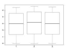
(a) 3 Boxplots of the 3 sets of $10^{4}$ simulated Bayes factors.

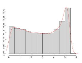
(b) Histogram of the sample of $3\cdot r$ Bayes factors and graph of its estimated density (red line).

(c) Prior density of $\delta$ with histogram of $10^{4}$ generated values.

Figure 2: Results of Case D1.

(a) 3 Boxplots of the 3 sets of $10^{4}$ simulated Bayes factors.

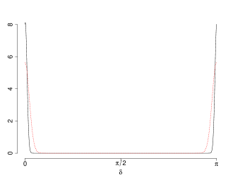
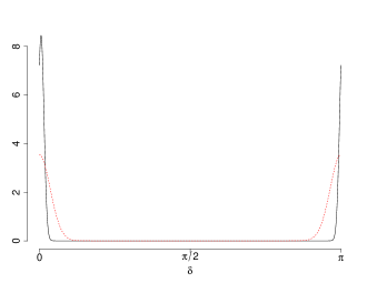
(b) Prior density (dashed line) and posterior density (continuous line) of $\delta$. The posterior is based on one generated sample.

Figure 3: Results of Case D1’.

Case D2 We now further decrease the concentration of the prior of $\delta$. The values of the hyperparameters are $\nu=0$ and $\tau=20$. We computed the prior probability of the null hypothesis under perturbation $p_{0}=0.176$. We generated the samples $\bm{\theta}^{(i)}$, for $i=1,\ldots,r$, with fixed value $\mu_{2}^{0}=0$.

We obtained three sequences of $r=10^{4}$ Bayes factors with means

$$\bar{B}_{01}^{(1)}=5.477,\bar{B}_{01}^{(2)}=5.539\;\text{ and }\bar{B}_{01}^{(3)}=5.511.$$

The boxplots of the three respective generated sequences are shown in Figure 4a. The asymptotic normal confidence interval for the mean value of the Bayes factors, at level 0.95 and based on the three generated sequences, is

$$(5.477,5.541).$$

The Bayes factors are larger than they are in Cases D1 and D1’. Here they show substantial evidence for the null hypothesis. The prior distribution $\delta$ is less favourable to the null hypothesis and so the sample brings more additional evidence for the null hypothesis. Figure 4b shows the graph of the prior density, as dashed line, together with the graph of a posterior density, as continuous line, for $\delta$. The graph of the posterior density is based on one generated sample.

(a) 3 Boxplots of the 3 sets of $10^{4}$ simulated Bayes factors.

(b) Prior density (dashed line) and posterior density (continuous line) of $\delta$. The posterior is based on one generated sample.

Figure 4: Results of Case D2.

3.1.2 Test of axial symmetry of GvM

In this section we consider the null hypothesis of axial symmetry, viz. $\text{H}_{0}$: $\delta=0$ or $\delta=\pi/2$, other parameters being fixed as follows, $\mu_{1}=\mu_{1}^{0},\kappa_{1}=\kappa_{1}^{0}$ and $\kappa_{2}=\kappa_{2}^{0}$. We choose as before $\mu_{1}^{0}=\pi$, $\kappa_{1}^{0}=0.1$ and $\kappa_{2}^{0}=5.5$. We generate $\delta$ from the prior given by the mixture of $\text{vM}_{2}$ distributions $\xi\,\text{vM}_{2}(\nu_{1},\tau)+(1-\xi)\,\text{vM}_{2}(\nu_{2},\tau)$, with $\nu_{1}=0,\nu_{2}=\pi/2$ and $\xi=0.5$. We consider three different cases, called Cases S1, S2 and S3.
Case S1 We generated $\delta$ from the prior mixture with concentration parameter $\tau=250$. This prior distribution is close to the null distribution and Figure 5b displays its density, together with the histogram of $10^{4}$ generations from it. We computed the prior probabilities of the null hypothesis under the perturbed probability measure $p_{0}=p_{\pi/2}=0.285$. We follow the principle of Case D1, where prior uncertainty is transmitted to the sample by considering generated values $\delta^{(i)}$, for $i=1,\ldots,s$, from a prior of $\delta$ close to the null hypothesis, instead of considering the fixed values of the null hypothesis, namely $\delta=0$ or $\pi/2$. We take the first $r$ of these prior values and we use $\mu_{2}^{(i)}=(\mu_{1}^{0}-\delta^{(i)})\leavevmode\nobreak\ \text{mod }\pi$ for generating $\bm{\theta}^{(i)}$, for $i=1,\ldots,r$. Repeating this three times, we obtained the three means of the three sequences of $r=10^{4}$ Bayes factors

$$\bar{B}_{01}^{(1)}=3.044,\bar{B}_{01}^{(2)}=2.986\text{ and }\bar{B}_{01}^{(3)}=2.950.$$

In Figure 5a we can find the boxplots of the three respective generated sequences. The asymptotic normal confidence interval for the mean value of the Bayes factors, at level 0.95 and based on the three generated sequences, is

$$(2.974,3.013).$$

The conclusion is that the sample provides positive evidence of axial symmetry, even though to some smaller extent only. The same was found in Case D1.

(a) 3 Boxplots of the 3 sets of $10^{4}$ simulated Bayes factors.

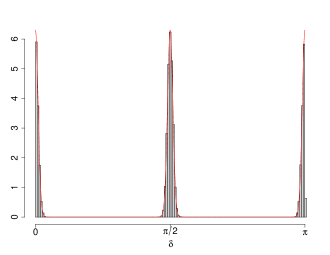
(b) Prior density of $\delta$ with histogram of $10^{4}$ generated values.

Figure 5: Results of Case S1.

(a) 3 Boxplots of the 3 sets of $10^{4}$ simulated Bayes factors.

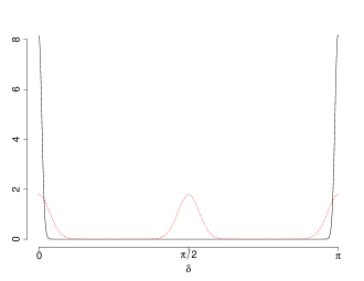
(b) Prior density (dashed line) and posterior density (continuous line) of $\delta$. The posterior is based on one generated sample.

Figure 6: Results of Case S2.

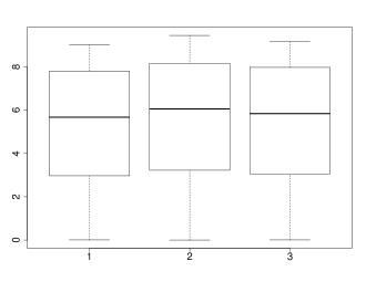
(a) 3 Boxplots of the 3 sets of $10^{4}$ simulated Bayes factors.

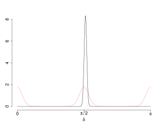
(b) Prior density (dashed line) and posterior density (continuous line) of $\delta$. The posterior is based on one generated sample.

Figure 7: Results of Case S3.

Case S2 We generated prior values of $\delta$ from the same mixture, however with smaller concentration hyperparameter $\tau=20$. We found $p_{0}=p_{\pi/2}=0.088$. We generated the elements of the sample vector $\bm{\theta}^{(i)}$ with fixed value $\mu_{2}^{0}=0$, thus from $\text{GvM}(\mu_{1}^{0},\mu_{2}^{0},\kappa_{1}^{0},\kappa_{2}^{0})$, with $\mu_{1}^{0}=\pi,\mu_{2}^{0}=0,\kappa_{1}^{0}=0.1,\kappa_{2}^{0}=5.5$, for $i=1,\ldots,r$. We repeated this experiment three times and obtained three sequences of Bayes factors, with respective mean values

$$\bar{B}_{01}^{(1)}=5.322,\bar{B}_{01}^{(2)}=5.439\;\text{ and }\bar{B}_{01}^{(3)}=5.282.$$

The boxplots of the three sequences of Bayes factors can be found in Figure 6a. After aggregating the three sequences, we obtained the asymptotic normal confidence interval at level $0.95$ for the mean value of the Bayes factors given by

$$(5.317,5.378).$$

The Bayes factor is thus larger than it was in Case S1, so that the sample has brought substantial evidence of axial symmetry. Figure (6b) shows the prior density of $\delta$ (dashed line) and a posterior density of $\delta$ (continuous line) that is based on one of the previously generated samples. The posterior is highly concentrated around $0$ and provides a stronger belief about symmetry than the prior.
Case S3 We retain the prior of $\delta$ of Case S2 but we generate samples $\bm{\theta}^{(i)}$, for $i=1,\ldots,r$, with $\mu_{1}^{0}=\pi,\mu_{2}^{0}=\pi/2,\kappa_{1}^{0}=0.1$, and $\kappa_{2}^{0}=5.5$, thus from another symmetric GvM distribution. The computed values $p_{0}=p_{\pi/2}=0.088$ are the same of Case S2. We generated three sequences of $r=10^{4}$ Bayes factors. The three respective boxplots of the three sequences can be found in 7a. The three respective means of these three sequences are

$$\bar{B}_{01}^{(1)}=5.267,\bar{B}_{01}^{(2)}=5.553\text{ and }\bar{B}_{01}^{(3)}=5.395.$$

By aggregating the three sequences, we obtained the asymptotic normal confidence interval at level $0.95$ for the mean of the Bayes factors given by

$$(5.374,5.436).$$

We find substantial evidence of axial symmetry. Figure 7b displays the prior density of $\delta$ (dashed line) and a posterior density of $\delta$ (continuous line) that is based on one of the previously generated samples. The posterior is highly concentrated around $\pi/2$ and possesses less uncertainty about symmetry than the prior.

3.1.3 Test of vM axial symmetry of GvM

Now we have $\text{H}_{0}:\kappa_{2}=0$, with fixed $\mu_{1}^{0}=\pi$, $\mu_{2}^{0}=\pi/2$ and $\kappa_{1}^{0}=0.1$. The prior distribution of $\kappa_{2}$ is uniform over $[0,1/2]$ and the sample $\bm{\theta}=(\theta_{1},\ldots,\theta_{n})$ is generated from the $\text{vM}(\mu_{1}^{0},\kappa_{1}^{0})$ distribution. The prior probability of $\text{H}_{0}$ under the perturbation is $p_{0}=0.1$. We generated three sequences of $r=10^{4}$ Bayes factors: their boxplots are shown in Figure 8. In these boxplots we removed a very small number of large values, in order to improve the readability. The three means of the three generated sequences are

$$B_{01}^{(1)}=3.284,\leavevmode\nobreak\ B_{01}^{(2)}=3.380\leavevmode\nobreak\ \text{ and }B_{01}^{(3)}=3.241,$$

where the very large values that were eliminated from the boxplots have been considered in the calculations of these means. After aggregating these three sequences, we obtained the following asymptotic normal confidence interval for the mean value of the Bayes factors at level $0.95$,

$$(3.268,3.335).$$

There is a positive evidence of symmetry although rather limited. The amount of evidence is similar to the cases D1 and S1: in all these studies, the prior is much concentrated around the null hypothesis (here $\kappa_{2}=0$), so that the data have increased the evidence of the null hypothesis only to some limited extend.

Figure 8: 3 boxplots of the 3 sets of $10^{4}$ simulated Bayes factors.

3.1.4 Summary

Table 2 summarizes the simulation results that we obtained for the three tests and for the various cases.

${\mbox{H}}_{0}$	case	confidence interval for $B_{01}$	evidence for ${\mbox{H}}_{0}$
no shift between cosines	D1	(2.937, 2.976)	positive
	D1’	(3.901, 3.945)	positive
	D2	(5.477, 5.541)	substantial
axial symmetry	S1	(2.974, 3.013)	positive
	S2	(5.317, 5.378)	substantial
	S3	(5.374, 5.436)	substantial
vM axial symmetry	–	(3.268, 3.335)	positive

Table 2: Summary of the simulation study.

3.2 Application to real data

The proposed Bayesian tests have been so far applied to simulated data. This section provides the application of the test of no shift between cosines of Section 2.2 and of axial symmetry of Section 2.3 to real data obtained from the study “ArticRIMS” (A Regional, Integrated Hydrological Monitoring System for the Pan Arctic Land Mass) available at http://rims.unh.edu. The Arctic climate, its vulnerability, its relation with the terrestrial biosphere and with the recent global climate change are the subjects under investigation. For this purpose, various meteorological variables such as temperature, precipitation, humidity, radiation, vapour pressure, speed and directions of winds are measured at four different sites.

We consider wind directions measured at the site “Europe basin” and from January to December 2005. After removal of few influential measurements, the following maximum likelihood estimators are obtained: $\hat{\mu_{1}}=4.095,\leavevmode\nobreak\ \leavevmode\nobreak\ \hat{\mu}_{2}=0.869,\leavevmode\nobreak\ \leavevmode\nobreak\ \hat{\kappa}_{1}=0.304,\leavevmode\nobreak\ \leavevmode\nobreak\ \hat{\kappa}_{2}=1.910$ and thus $\hat{\delta}=(\hat{\mu_{1}}-\hat{\mu}_{2})\text{ mod }\pi=0.084$. The histogram of the sample together with the GvM density with theses values of the parameters are given in Figure 9.

For the test of no shift between cosines, the Monte Carlo integral (13) is computed with $s=10^{6}$ values of $\delta$ generated from the prior $\text{vM}_{2}(\nu,\tau)$, with $\nu=0$ and $\tau=300$. We consider $\varepsilon=0.18$: as mentioned in Section 2.1, a substantial value is desirable in the practice. We obtain the Bayes factor $B_{01}=2.550$; cf. Table 3.

For the test of symmetry, the prior of $\delta$ is the mixture of two vM of order two, i.e. $\xi\,\text{vM}_{2}(\nu_{1},\tau)+(1-\xi)\,\text{vM}_{2}(\nu_{2},\tau)$, with $\nu_{1}=0,\leavevmode\nobreak\ \nu_{2}=\pi/2,\leavevmode\nobreak\ \tau=300$ and $\xi=0.5$. Monte Carlo integration is done with $s=10^{6}$ generations from this prior. We consider $\varepsilon=0.18$ and obtain the Bayes factor $B_{01}=2.252$; cf. Table 3.

The values of the two Bayes factors of Table 3 show positive evidence for the respective null hypotheses.

$\text{H}_{0}$	$B_{01}$	evidence for $\text{H}_{0}$
no shift between cosines	2.550	positive
axial symmetry	2.252	positive

Table 3: Bayes factors for wind directions data.

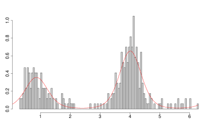
Figure 9: Histogram of wind directions data together with $\text{GvM}(\hat{\mu}_{1},\hat{\mu}_{2},\hat{\kappa}_{1},\hat{\kappa}_{2})$ density.

4 Conclusion

This article introduces three Bayesian tests relating to the symmetry of the GvM model. The first test is about the significance of the shift parameter between the cosines of frequency one and two (${\mbox{H}}_{0}:\delta=0$). The second test is about axial symmetry (${\mbox{H}}_{0}:\delta=0$ or $\delta=\pi/2$). The third test is about vM symmetry ($\text{H}_{0}:\kappa_{2}=0$). These tests are obtained by the technique of probability perturbation. Simulation studies show the effectiveness of these three tests, in the sense that when the sample is coherent with the null hypothesis, then the Bayes factors are typically large. Applications to real data are also shown.

Due to computational limitations, we consider null hypotheses of symmetry that concern one parameter only. The null hypotheses considered are about one or two distinct values of the parameter of interest, with all remaining parameters fixed. Composite null hypotheses that allow for unknown nuisance parameters, would require one additional dimension of Monte Carlo integration for each unknown parameter, in the computation of the marginal distribution. The computational burden would rise substantially and the Monte Carlo study, with two levels of nested generations, would become very difficult. But the essentially simple null hypotheses considered are relevant in the practice. It can happen that nuisance parameters have been accurately estimated and the question of interest is really about the the parameter $\delta$ and axial symmetry. In the example of Section 3.2, we want to know if wind direction is axially symmetric within the GvM model. The values of the concentrations and of the axial direction are of secondary importance.

One could derive other Bayesian tests for the GvM model: a Bayesian test of bimodality is under investigation. We can also note that Navarro et al., (2017) introduced an useful multivariate GvM distribution for which similar Bayesian tests could be investigated.

The computations of this article are done with the language R, see R Development Core Team, (2008), over a computing cluster with several cores. The programs are available at the software section of http://www.stat.unibe.ch.

Appendix A Proof of Proposition 2.1

The definition of axial symmetry given at the beginning of Section 2.3 tells that the GvM distribution is symmetric around $\alpha/2$ (or $\alpha/2+\pi$), for some $\alpha\in[0,2\pi)$, iff

$$f(\theta|\mu_{1},\mu_{2},\kappa_{1},\kappa_{2})=f(\alpha-\theta|\mu_{1},\mu_{2},\kappa_{1},\kappa_{2}),\leavevmode\nobreak\ \leavevmode\nobreak\ \forall\theta\in[0,2\pi).$$

This means

$$\begin{split}\kappa_{1}\cos(\theta-\mu_{1})+\kappa_{2}\cos 2(\theta-\mu_{2})&=\kappa_{1}\cos[(\alpha-\theta)-\mu_{1}]+\kappa_{2}\cos 2[(\alpha-\theta)-\mu_{2}]\\ &=\kappa_{1}\cos[\theta-(\alpha-\mu_{1})]+\kappa_{2}\cos 2[\theta-(\alpha-\mu_{2})],\end{split}$$ (19)

$\forall\theta\in[0,2\pi)$. By using the cosine addition formula, (19) can be re-expressed as

$$\begin{split}\kappa_{1}\cos\theta\cos\mu_{1}+\kappa_{1}\sin\theta\sin\mu_{1}+\kappa_{2}\cos 2\theta\cos 2\mu_{2}+\kappa_{2}\sin 2\theta\sin 2\mu_{2}=\qquad\qquad\qquad\qquad\qquad\\ \kappa_{1}\cos\theta\cos(\alpha-\mu_{1})+\kappa_{1}\sin\theta\sin(\alpha-\mu_{1})+\kappa_{2}\cos 2\theta\cos 2(\alpha-\mu_{2})+\kappa_{2}\sin 2\theta\sin 2(\alpha-\mu_{2}),\end{split}$$

$\forall\theta\in[0,2\pi)$. This is equivalent to the equation

$$\begin{split}&\kappa_{1}[\cos\mu_{1}-\cos(\alpha-\mu_{1})]\cos\theta+\kappa_{2}[\cos 2\mu_{2}-\cos 2(\alpha-\mu_{2})]\cos 2\theta\\ &\qquad+\kappa_{1}[\sin\mu_{1}-\sin(\alpha-\mu_{1})]\sin\theta+\kappa_{2}[\sin 2\mu_{2}-\sin 2(\alpha-\mu_{2})]\sin 2\theta=0,\end{split}$$

$\forall\theta\in[0,2\pi)$. It is convenient to re-express this last equation in terms of a trigonometric polynomial of degree $N=2$, precisely as

$$p(\theta)=\sum_{j=1}^{N}(a_{j}\cos j\theta+b_{j}\sin j\theta)=0,\leavevmode\nobreak\ \forall\theta\in[0,2\pi),$$ (20)

whose coefficients are given by

$$a_{j} =\kappa_{j}[\cos j\mu_{j}-\cos j(\alpha-\mu_{j})]\;\text{ and }\;b_{j}=\kappa_{j}[\sin j\mu_{j}-\sin j(\alpha-\mu_{j})],\text{ for }j=1,2.$$

A trigonometric polynomial of degree $N$ has maximum $2N$ roots in $[0,2\pi)$, unless it is the null polynomial; see e.g. p. 150 of Powell, (1981). With this, (20) implies that $p(\theta)$ is the null polynomial, which means that $a_{j}=b_{j}=0$, for $j=1,2$. These four equalities give the system of equations

$$\begin{cases}\cos\mu_{1}=\cos(\alpha-\mu_{1}),\\ \sin\mu_{1}=\sin(\alpha-\mu_{1}),\\ \cos 2\mu_{2}=\cos 2(\alpha-\mu_{2}),\\ \sin 2\mu_{2}=\sin 2(\alpha-\mu_{2}),\end{cases}$$

which, in terms of $\delta=(\mu_{1}-\mu_{2})\mbox{\rm mod}\pi$, simplifies to

$$\begin{cases}\alpha=2\mu_{1}+2k\pi,\\ \alpha=2\big{[}(\mu_{1}-\delta)\leavevmode\nobreak\ \text{mod $\pi$}\big{]}+k_{1}\pi,\end{cases}\;\text{ for some }k,k_{1}\in\mathbb{Z}.$$

One can eliminate the congruence symbol mod and obtain

$$\begin{cases}\alpha=2\mu_{1}+2k\pi,\\ \alpha=2\mu_{1}-2\delta+(k_{1}+2k_{2})\pi,\end{cases}\;\text{ for some }k,k_{1},k_{2}\in\mathbb{Z}.$$ (21)

This system of simultaneous equation admits solutions iff $2\delta$ is a multiple of $\pi$, i.e. $2\delta=0\leavevmode\nobreak\ \text{mod $\pi$}$. Since $\delta\in[0,\pi)$, we have found the desired symmetry characterization.

References

- Abe et al., (2013) Abe, T., Pewsey, A., and Shimizu, K. (2013). Extending circular distributions through transformation of argument. Annals of the Institute of Statistical Mathematics, 65(5):833–858.
- Abramowitz and Stegun, (1972) Abramowitz, M. and Stegun, I. (1972). Handbook of mathematical functions (tenth printing ed.). United States Department of Commerce.
- Astfalck et al., (2018) Astfalck, L., Cripps, E., Gosling, J., Hodkiewicz, M., and Milne, I. (2018). Expert elicitation of directional metocean parameters. Ocean Engineering, 161:268–276.
- Batschelet, (1981) Batschelet, E. (1981). Circular statistics in biology. Academic Press, New York.
- Berger, (1985) Berger, J. O. (1985). Statistical decision theory and Bayesian analysis. Springer Science & Business Media.
- Berger and Delampady, (1987) Berger, J. O. and Delampady, M. (1987). Testing precise hypotheses. Statistical Science, pages 317–335.
- Berger and Sellke, (1987) Berger, J. O. and Sellke, T. (1987). Testing a point null hypothesis: The irreconcilability of p values and evidence. Journal of the American statistical Association, 82(397):112–122.
- Christmas, (2014) Christmas, J. (2014). Bayesian spectral analysis with student-t noise. IEEE Transactions on Signal Processing, 62(11):2871–2878.
- Gatto, (2008) Gatto, R. (2008). Some computational aspects of the generalized von Mises distribution. Statistics and Computing, 18(3):321–331.
- Gatto, (2009) Gatto, R. (2009). Information theoretic results for circular distributions. Statistics, 43(4):409–421.
- Gatto, (2021) Gatto, R. (2021). Information theoretic results for stationary time series and the Gaussian-generalized von Mises time series. Selected Papers for the Bicentennial Birth Anniversary of F. Nightingale, editors B. Arnold and A. SenGupta, Springer, to appear.
- Gatto and Jammalamadaka, (2003) Gatto, R. and Jammalamadaka, S. R. (2003). Inference for wrapped symmetric -stable circular models. Sankhyā: The Indian Journal of Statistics, pages 333–355.
- Gatto and Jammalamadaka, (2007) Gatto, R. and Jammalamadaka, S. R. (2007). The generalized von Mises distribution. Statistical Methodology, 4(3):341–353.
- Gatto and Jammalamadaka, (2014) Gatto, R. and Jammalamadaka, S. R. (2014). Directional statistics: introduction. Wiley StatsRef: Statistics Reference Online, pages 1–8.
- Jammalamadaka and SenGupta, (2001) Jammalamadaka, S. R. and SenGupta, A. (2001). Topics in circular statistics, volume 5. World Scientific.
- Jeffreys, (1961) Jeffreys, H. (1961). Theory of probability. Oxford University Press, London.
- Kass and Raftery, (1995) Kass, R. E. and Raftery, A. E. (1995). Bayes factors. Journal of the american statistical association, 90(430):773–795.
- Kass and Wasserman, (1996) Kass, R. E. and Wasserman, L. (1996). The selection of prior distributions by formal rules. Journal of the American statistical Association, 91(435):1343–1370.
- Kato and Jones, (2015) Kato, S. and Jones, M. (2015). A tractable and interpretable four-parameter family of unimodal distributions on the circle. Biometrika, 102(1):181–190.
- Ley and Verdebout, (2017) Ley, C. and Verdebout, T. (2017). Modern directional statistics. CRC Press.
- Ley and Verdebout, (2018) Ley, C. and Verdebout, T. (2018). Applied directional statistics: Modern methods and case studies. CRC Press.
- Lin and Dong, (2019) Lin, Y. and Dong, S. (2019). Wave energy assessment based on trivariate distribution of significant wave height, mean period and direction. Applied Ocean Research, 87:47–63.
- Lindley, (1977) Lindley, D. V. (1977). A problem in forensic science. Biometrika, 64(2):207–213.
- Mardia and Jupp, (2000) Mardia, K. V. and Jupp, P. E. (2000). Directional statistics, volume 494. John Wiley & Sons.
- Navarro et al., (2017) Navarro, A., Frellsen, J., and Turner, R. (2017). The Multivariate Generalised von Mises Distribution: Inference and Applications. In Thirty-First AAAI Conference on Artificial Intelligence.
- Pewsey, (2002) Pewsey, A. (2002). Testing circular symmetry. Canadian Journal of Statistics, 30(4):591–600.
- Pewsey, (2004) Pewsey, A. (2004). Testing for circular reflective symmetry about a known median axis. Journal of Applied Statistics, 31:575–585.
- Pewsey et al., (2013) Pewsey, A., Neuhäuser, M., and Ruxton, G. D. (2013). Circular statistics in R. Oxford University Press.
- Powell, (1981) Powell, M. J. D. (1981). Approximation theory and methods. Cambridge University press.
- R Development Core Team, (2008) R Development Core Team (2008). R: A Language and Environment for Statistical Computing. R Foundation for Statistical Computing, Vienna, Austria.
- Spurr and Koutbeiy, (1991) Spurr, B. D. and Koutbeiy, M. A. (1991). A comparison of various methods for estimating the parameters in mixtures of von Mises distributions. Communications in Statistics-Simulation and Computation, 20(2-3):725–741.
- Umbach and Jammalamadaka, (2009) Umbach, D. and Jammalamadaka, S. R. (2009). Building asymmetry into circular distributions. Statistics & Probability Letters, 79(5):659–663.
- Zellner, (1984) Zellner, A. (1984). Posterior odds ratios for regression hypotheses: General considerations and some specific results. Basic Issues in Econometrics (A.Zellner, ed), pages 275–305.
- Zhang et al., (2018) Zhang, L., Li, Q., Guo, Y., Yang, Z., and Zhang, L. (2018). An investigation of wind direction and speed in a featured wind farm using joint probability distribution methods. Sustainability, 10(12).