Absence of Phase Transition in Random Language Model
Abstract
The Random Language Model, proposed as a simple model of human languages, is defined by the averaged model of a probabilistic context-free grammar. This grammar expresses the process of sentence generation as a tree graph with nodes having symbols as variables. Previous studies proposed that a phase transition, which can be considered to represent the emergence of order in language, occurs in the random language model. We discuss theoretically that the analysis of the “order parameter” introduced in previous studies can be reduced to solving the maximum eigenvector of the transition probability matrix determined by a grammar. This helps analyze the distribution of a quantity determining the behavior of the “order parameter” and reveals that no phase transition occurs. Our results suggest the need to study a more complex model such as a probabilistic context-sensitive grammar, in order for phase transitions to occur.
I Introduction
Chomsky attempted to establish formal models that represent the universal grammar underlying all languages [1, 2]. One such model is a context-free grammar (CFG) [3], which has been used beyond the scope of linguistic research in various fields such as quasicrystal[4] and molecular optimization[5]. To better understand natural languages, a possible extension of this abstract model is a probabilistic version, called probabilistic context-free grammar (PCFG) [6], which has been studied as a model of cosmic inflation [7], recurrent neural network [8], a prior distribution of RNA secondary structures [9], etc. However, partly because Chomsky strongly denied the importance of statistical approaches to language, limited research has been conducted on PCFG in the context of understanding natural languages. Several studies [10, 11, 12] on grammar induction and parsing based on PCFG, which are analogies for how humans acquire and recognize their first language, focus on specific corpora and not on the universal or typical properties of languages.
Recently, DeGiuli, in their study on the typical properties of PCFG, introduced a model of averaged PCFG, called the Random Language Model (RLM)[13]. This model can be viewed as a statistical-mechanical model of random systems, which helps derive the free energy formula of the model using theoretical physics methods, such as the replica method and Feynman diagrams[14]. Numerical simulations and statistical-mechanical analyses of the model suggest that a phase transition occurs between ordered and random phases as the model parameters vary, demonstrating the emergence of order in language just as a child initially speaks incoherently, but later learns to speak grammatically correct language. The presence of the phase transition would implies that the difference between children’s incoherent “languages” and adults’ languages is not quantitative but qualitative. However, the previous analyses do not prove the existence of the phase transition. We address this issue because it is a fundamental problem whether a phase transition exists in a simple model such as the RLM.
This article is organized as follows: in Sec. II, the models we discuss, i.e., CFG, PCFG, and RLM, are described step by step, and the “order parameter” introduced in the previous study[13] to detect a phase transition in the RLM is presented. Sec. III is the main content of this article where we examine the possibility of the phase transition by analyzing the “order parameter.” We point out that the probability of occurrence of a symbol is an essential quantity characterizing the RLM, and our analyses in terms of the probability reveal that the phase transition cannot exist. In other words, the RLM only presents a crossover. We also discuss how the crossover occurs. In Sec.IV, we summarize the results and imply the need to study a more complex model with context-sensitiveness. The appendices provide further details on our analysis and Shannon entropy.
II Models and “order parameter”
II.1 Context-free Grammar
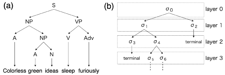
A conventional approach in linguistics is to analyze syntactic structures underlying sentences in terms of immediate constituent (IC) analyses. In this framework, these structures are represented graphically by tree diagrams as shown in Fig. 1(a) [1]. CFG or type 2 grammar is a formal grammar which generates sentences with such tree-like structures [3, 2]. The CFG consists of a set of symbols called a vocabulary or an alphabet, and a set of rules. The vocabulary is the union of two disjoint finite sets and , which are sets of nonterminal and terminal symbols, respectively. Each rule in is of the form , i.e., an instruction to rewrite a single nonterminal symbol as a string in . Given the special nonterminal symbol , called a starting symbol, one applies rules in iteratively until the string comprises solely terminal symbols. This final string of terminal symbols is defined as a sentence generated by . Furthermore, the complete process of generating a sentence is called a derivation. A derivation is represented as a tree as in IC analyses, the leaves of which represent the sentence. In linguistics, nonterminal symbols correspond to constituents or phrases such as sentences, noun phrases, or verb phrases, while terminal symbols correspond to words or morphemes, such as “ideas” or “sleep”. Although CFG does not explain all aspects of natural languages, it reflects the fundamental structure of a class called kernel comprising basic sentences such as active and declarative sentences. Without the loss of generality, one can restrict rules to the form and , where , , and are nonterminal symbols and is a terminal symbol [15]. We shall call them nonterminal rules and terminal rules, respectively.
II.2 probabilistic Context-free Grammar
Sentences we generate depend not only on the grammar, but also on the intentions of speakers or writers and situations where they are generated. However, for simplicity, we consider the model in which sentences are generated randomly according to given probabilistic weights and CFG, i.e., PCFG [6]. We assign weight to each , and to each . and define the probability that nonterminal symbol is rewritten by nonterminal rule and terminal rule , respectively. Notice that or in PCFG corresponds to the situation that does not include or in CFG. The sets and of weights determine the probability with which each sentence or derivation is generated. With fixed , each PCFG is only characterized by and .
According to [13, 14], we introduce the “emission probability” , which is the probability that a nonterminal symbol is rewritten as a terminal symbol, and redefine weights and such that the probability for and are and , respectively. In this setup, the topology of a derivation is independent of the occurrence of symbols on , and is only controlled by the emission probability .
II.3 Random Language Model
We are interested in typical properties of a general language, not of a particular language. To analyze the typical properties, we consider an averaged model, assuming that weights are generated randomly according to some distribution . The introduction of the emission probability allows us to divide into and . As these distributions, we choose lognormals:
| (1) |
where and are parameters that characterize the prior distributions. This is the RLM introduced by DeGiuli[13, 14].
II.4 “Order Parameter”
In the previous studies, to clarify the behavior of the RLM, the “order parameter” is introduced as
where is the number of applications of nonterminal rules in a derivation. , , and are the indices of nodes of given , and is a nonterminal symbol on node . The summation runs over all such that is applied in a derivation. denotes the average over derivations generated according to weights and the emission probability . Note that we do not need to consider weights as long as we focus on because this parameter depends only on the structure of nonterminal symbols. This definition is motivated by that of the order parameter for Potts model[16].
Numerical simulations of this quantity suggest the existence of a phase transition with a change in the parameter . The transition point separates a random phase and an ordered phase. In the former, the averaged sum of squared “order parameters” is vanishingly small, where means the average over weights according to . Meanwhile, in the latter, it takes a finite value. This may be interpreted as an indication of the emergence of nontrivial order, which allows sentences to communicate information. However, the origin and characteristics of the singularity associated with a phase transition are not always evident. Indeed, the previous studies present no concrete evidences for the phase transition.
III Analysis
III.1 Probability of Occurrence of Symbol
In this paper, we theoretically revisit the phase transition in the RLM from a viewpoint different from that of previous studies. The key point is that the singularity of “order parameter” is reduced to that of the probability of occurrence of symbol . First, we denote this as
where the nonterminal symbols rewritten by terminal rules are not counted in both the numerator and the dominator. The “order parameter” can be rewritten as
| (2) |
Because the distribution is an analytic function of , the behavior of factor is also analytic. Thus, the order parameter will not present any singularity unless the distribution of non-analytically changes.
For the analysis of , it is useful to decompose a tree into layers from the root to leaves, as shown in Fig. 1(b). In addition, we denote the number of nodes and occurrence of symbol in layer , except those turning into terminal symbols in layer , as and , respectively. In terms of these, is represented as
| (3) |
where . Recall that the topology of a derivation is generated independently of the occurrence of symbols on . Therefore, we can average over the occurrence of symbols up to layer before the topology in the computation of the summand, represented as
Considering the process of developing the layers, the transition probability that a symbol in layer turns into a symbol in layer is given by
Using the transition matrix , it turns out
where and . Notice that is the distribution of starting symbols. The right hand side of the above equation is independent of the topology . Combining these, the summand of Eq. (3) yields
| (4) | ||||
| (5) |
It would be interesting to see that Eq. (3) is separated into the product form of the dependencies on and .
III.2 Case of
The factor can be expressed in terms of a moment generating function (see Appendix A). For general , it is difficult to write it down explicitly, but in the special case of , the following argument can be proceeded. In this case, and . Substituting these into Eq. (3) and (4), it turns out that , where is the steady state of the Markov chain defined by . Because is a transition probability matrix, corresponds to the unique maximum eigenvector of belonging to eigenvalue 1 with probability if . As a consequence, it turns out that for , it is sufficient to find the largest eigenvector of to analyze the “order parameter” of a given grammar . For , it is convenient to define a set for each , where means that in for any . The probability density of is expressed as . Because the measure is an analytic function of defined by Eq. (1), is also analytic with . This means that a phase transition detected by the “order parameter” cannot exist.
III.3 Case of
For , how does the distribution of behave when changes? As increases, for small increases while that for large decreases, and thus gets closer to since for smaller is closer to . It is unlikely that this effect leads to a singularity. This implies that no phase transition exists not only for but also for general .
To confirm the above argument quantitatively, we measured numerically the Binder parameter of , defined as
| (6) |
where . This parameter has been used to numerically detect the transition temperature of first- and second-order transitions in various statistical-mechanical models [17, 18, 18]. For all previously known cases of phase transitions detected by this parameter, a discontinuous jump from zero implying a Gaussian distribution to a finite value determined by a multimodal distribution is found at the transition temperature in the thermodynamic limit.
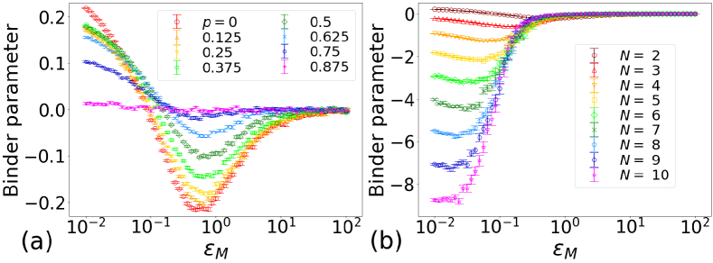
Fig. 2 (a) shows the Binder parameters of for with several values of the emission probability . For , we directly calculated for the derivations of the maximum depth , i.e., those of infinite sizes, using the solution of the maximum eigenvector problem of transition probability matrix . This is a significant advantage of the fact that . For , we measured by implementing the RLM. Because it is impossible to generate a derivation of infinite size, we measured with the maximum depth instead, which was sufficient to approximate the Binder parameter for . We chose for any symbol as the distribution of starting symbols, thus the Binder parameter of is zero. The number of grammars generated for each was for both and . In addition, derivations were generated for each grammar for . In this figure, the Binder parameter for is shown to be analytic in , which is predicted from the above analysis concluding that the distribution is analytic. It should be emphasized that this plot is calculated directly in terms of eigenvalue analysis, not approximated by generating derivations of finite sizes. This plot means that the Binder parameter at is truly analytic for an infinite system, not that it appears to be analytic because of finite system. From this figure, we can also see that the Binder parameter get closer to zero, with no singularities for any , as increases. This is consistent with the above argument that there is no phase transition for .
Note that the distribution may have a singularity with respect to at , caused by percolation transition[20]. However, even if this transition exists, we will be able to explain it as a phenomenon of a tree branching probabilistically, and this singularity has no relation to the weights which is the essential element of PCFG. This transition would not reflect any nature of PCFG.
III.4 Mechanism of Crossover
Even if a quantity does not present a phase transition, it will be an interesting problem how the quantity crosses over. The fact that for helps understand the behavior of at . In the limit, for any , , and is with probability 1, leading to for any and , and the maximum eigenvector is . This implies . Meanwhile, for the , one element of ’s is 1 and the other elements are 0 for each with probability 1. Thus, the number of possible is the same as the choice of the elements of value 1, and the numbers of possible and the corresponding are finite. Thus, has multiple delta peaks. Note that the maximum eigenvector is not unique and depends on the initial state in this case. In the intermediate region , is a continuous function of because is that of . If turned discontinuously from single delta peak to multiple ones at finite , it would be a phase transition similar to that with one-step replica symmetry-breaking[21, 22]. However, becomes a delta function only at and .
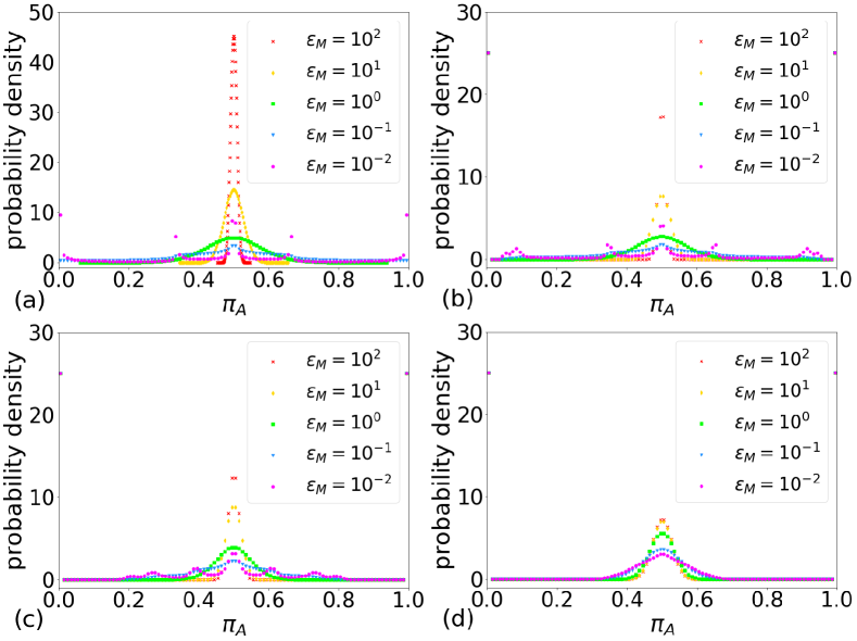
We actually computed and observed the distribution for and through numerical simulations. As in measurement of the Binder parameters, for was computed through eigenvalue analysis while that for was approximated implementing the RLM with the fixed maximum depth . We assumed for any nonterminal symbol . In addition, we generated grammars for each for both and and derivations for each grammar for . Fig. 3(a) shows the plots for . for has a single peak around , meaning that symbols occur according to almost uniform distribution under many grammars. Meanwhile, for small , is multimodal, because various grammars are generated and their distributions of symbols are different depending on grammars. However, we emphasize that is not a delta function for finite as discussed in the preceding paragraph. This figure also show that the dip of the Binder parameter in Fig. 2 occurs around the point at which turns from single peak to multiple peaks. From Fig. 3(b), (c), and (d), it can be seen that becomes closer to Gaussian centered at as increases. This is also consistent with the above discussion.
III.5 The Limit
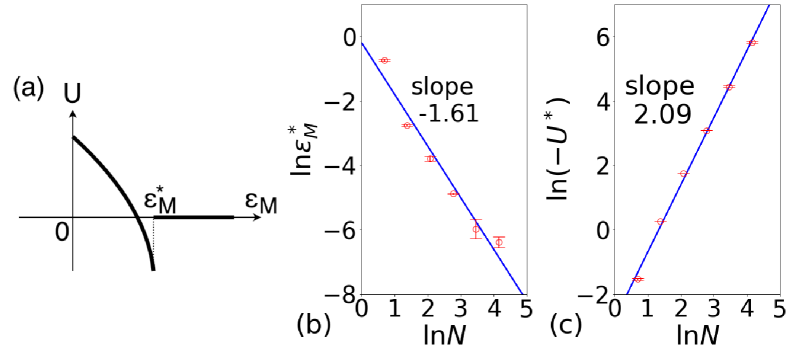
It is revealed that there is no phase transition for finite . We now consider the possibility of existence of phase transition in the limit . If we agree with the concept of the so-called infinite use of finite means, the essential characteristic of language is that it can express infinite meanings with finite symbols[1, 23]. From this viewpoint, it is not clear what property of language this limit explains. Still, this limit is interesting as a physical model, since PCFG is used as a model for various phenomena other than language. As we have shown, it is sufficient to deal with the case with for the investigation of whether a phase transition exists. Fig. 2(b) shows the Binder parameters of for and . For each , grammars for and grammars for were generated. As seen in Fig. 2(b), the dip of the Binder parameter gets deeper as increases. In the limit , this point might become singular at finite shown in Fig. 4(a), which can be a phase transition as seen in a three-dimensional Heisenberg spin glass [24].
To study whether this phenomenon occurs, we observed numerically the dependence of the local minimum point of the Binder parameter on by generating grammars for each and . As Fig. 4(b) and (c) show, the results suggest that converges to zero algebraically in and also diverges to algebraically. Thus, no evidences imply the existence of singularity as in Fig. 4(a) in the limit .
IV Conclusion
Our analysis for finite holds even if the weights are not generated from a lognormal distribution. As long as the distribution is an analytic function of , the analyticity of can be shown theoretically in the same way. Our numerical analysis for infinite also suggests that no phase transition exists even in the limit . This conclusion might be different if the distribution of is not the lognormal distribution. For example, if ’s are not i.i.d., but dependent on each other, then might have a singularity with respect to in the limit . In Ref. [13], DeGiuli also claimed that Shannon entropy has a singularity. However, an argument similar to that for the “order parameter” can be developed to show the analyticity of Shannon entropy. The detailed explanation is presented in Appendix B.
In terms of both the “order parameter” and Shannon entropy, the RLM does not have a singularity. This may imply that children’s languages and adults’ languages are different only quantitatively, not qualitatively. As seen from the overall analysis, the most fundamental reason for the absence of singularity relies on the fact that the distribution of a symbol on a node depends only on the weights and the distribution on its parent node. To see a nontrivial physical phenomenon such as a phase transition, we might need to consider more complex models in which the distribution on a node is determined by more factors. One possible model is probabilistic context-sensitive grammar (PCSG), that is, an extension of context-sensitive grammar (CSG) by assigning probabilistic weights to the rules. CSG is one level higher than CFG in the Chomsky hierarchy[3], where a resulting string in each rule depends not on a single symbol, but on a substring. Thanks to this property, the behavior of the distribution of symbols can no longer be computed in the same manner as in PCFG.
We conclude that, in the RLM, the model for the typical evaluation of PCFG, there does not exist a phase transition as has been suggested, because the PCFG and the RLM are too simple. This fact may imply that language acquisition of children is a continuous process. The absence of the nontrivial phenomenon, i.e., a phase transition, does not deny the significance of the study of the probabilistic extension of grammars in the Chomsky hierarchy as an approach for natural language from mathematical sciences. The typical properties of PCSG should be analyzed in the future to search for the nontrivial physical phenomena that are different from those in the RLM.
Acknowledgements.
We would like to thank K. Kaneko, A. Ikeda, and A. Morihata for useful discussions. This work was partly supported by the World-leading Innovative Graduate Study Program for Advanced Basic Science Course at the University of Tokyo.Appendix A Moment generating function for computing
The function is defined by
where is the number of nonterminal symbols to which nonterminal rules apply in layer . This function can be computed by differentiating and integrating the following moment generating function:
| (7) |
Indeed, the relation between and is as follows:
Because only depends on , we can take the expectation in the right-hand side of Eq. (7) one by one from to . First, the expectation over is taken, we have
where is the number of nonterminal symbols in layer that change to terminal symbols in the next layer. Thus, it yields
where
| (8) |
By repeating the same calculation for sequentially, we can finally obtain
where is defined recursively by Eq. (8) and
for .
Appendix B Analyticity of Shannon Entropy
In [13], DeGiuli also focused on Shannon entropy of a sequence of symbols on any fixed nodes , which we denote as
| (9) |
With numerical simulations, DeGiuli suggested that this quantity has a singularity with at the same point where the “order parameter” does, that is, the averaged Shannon entropy is equivalent to that expected from strings generated uniformly at random above the transition point and substantially smaller than it below the point. We consider whether this expectation is relevant or not.
From Eq. (9), Shannon entropy will not have a singularity if the joint probability is analytic. To investigate the joint probability, we introduce the conditional probability that the symbol on node is , on the condition that the symbol on the ancestor of node is . The joint probability can be represented using weights , the distribution of a starting symbol, and the conditional probability . Consider the case where the number of nodes is , i.e., . For any fixed and , the lowest node of the common ancestors of them uniquely exists, and we denote it as . The node has the two children, one of which is the ancestor of node , and the other of which is that of node , denoted and , respectively. The joint probability is represented as
| (10) |
The joint probability for is represented with an argument similar to that given above.
The matrix can be written as a product of transition probability matrices. We label the indices of nodes between and as and such that node is the parent of node for . Next, we define matrices and by
respectively. Using these notations, the matrix is
| (11) |
where is if node is the left child of node , while is if node is the right child.
Combining Eq. (10) and (11), we can compute the joint probability as a product of , , , and . Thus, if the distance between root node and a node in is finite, this joint probability is analytic for any analytic distribution of . If the distance is infinite, the joint probability is mainly determined by a kind of steady state of the sequence of transition probability matrices in the way similar to that in the case with the “order parameter” . This implies that Shannon entropy also does not have a singularity with .
References
- Chomsky [1957] N. Chomsky, Syntactic Structures (Mouton & Co., 1957).
- Chomsky [1956] N. Chomsky, Three models for the description of language, IRE Transactions on information theory 2, 113 (1956).
- Chomsky [1959] N. Chomsky, On certain formal properties of grammars, Information and control 2, 137 (1959).
- Escudero [1997] J. G. Escudero, Formal languages for quasicrystals, in Symmetries in Science IX (Springer, 1997) pp. 139–152.
- Kajino [2019] H. Kajino, Molecular hypergraph grammar with its application to molecular optimization, in International Conference on Machine Learning (PMLR, 2019) pp. 3183–3191.
- Jelinek et al. [1992] F. Jelinek, J. D. Lafferty, and R. Mercer, Basic methods of probabilistic context free grammars, in Speech Recognition and Understanding (Springer, 1992) pp. 345–360.
- Harlow et al. [2012] D. Harlow, S. H. Shenker, D. Stanford, and L. Susskind, Tree-like structure of eternal inflation: A solvable model, Phys. Rev. D 85, 063516 (2012).
- Lin and Tegmark [2017] H. W. Lin and M. Tegmark, Critical behavior in physics and probabilistic formal languages, Entropy 19, 299 (2017).
- Knudsen and Hein [1999] B. Knudsen and J. Hein, Rna secondary structure prediction using stochastic context-free grammars and evolutionary history., Bioinformatics 15, 446 (1999).
- Klein and Manning [2004] D. Klein and C. D. Manning, Corpus-based induction of syntactic structure: Models of dependency and constituency, in Proceedings of the 42nd annual meeting of the association for computational linguistics (ACL-04) (2004) pp. 478–485.
- Noji [2016] H. Noji, Statistical models to induce latent syntactic structures, Proceedings of the Institute of Statistical Mathematics 64, 145 (2016).
- Ney [1991] H. Ney, Dynamic programming parsing for context-free grammars in continuous speech recognition, IEEE Transactions on Signal Processing 39, 336 (1991).
- DeGiuli [2019a] E. DeGiuli, Random language model, Phys. Rev. Lett. 122, 128301 (2019a).
- DeGiuli [2019b] E. DeGiuli, Emergence of order in random languages, J. Phys. A 52, 504001 (2019b).
- Hopcroft et al. [2007] J. E. Hopcroft, R. Motwani, and J. Ullman, Introduction to Automata Theory, Languages, and Computation, 3rd ed. (Pearson, 2007).
- Gross et al. [1985] D. J. Gross, I. Kanter, and H. Sompolinsky, Mean-field theory of the potts glass, Phys. Rev. Lett. 55, 304 (1985).
- Binder [1981] K. Binder, Finite size scaling analysis of ising model block distribution functions, Z. Phys. B 43, 119 (1981).
- Binder and D.P.Landau [1984] K. Binder and D.P.Landau, Finite-size scaling at first-order phase transitions, Phys. Rev. B 30, 1477 (1984).
- Young [2012] P. Young, Everything you wanted to know about data analysis and fitting but were afraid to ask, e-print arXiv:1210.3781 (2012).
- Stauffer and Aharony [2018] D. Stauffer and A. Aharony, Introduction to Percolation Theory (CRC press, 2018).
- Binder and Young [1986] K. Binder and A. P. Young, Spin glasses: Experimental facts, theoretical concepts, and open questions, Rev. Mod. Phys. 58, 801 (1986).
- Mezard et al. [1986] M. Mezard, G. Parisi, M. Virasoro, and N. Chomsky, Spin Glass Theory and Beyond (World Scientific Lecture Notes in Physics: Volume 9, 1986).
- Yang et al. [2017] C. Yang, S. Crain, R. C. Berwick, N. Chomsky, and J. J. Bolhuis, The growth of language: Universal grammar, experience, and principles of computation, Neurosci. Biobehav. Rev. 81, 103 (2017).
- Imagawa and Kawamura [2002] D. Imagawa and H. Kawamura, Monte carlo studies of the ordering of the three-dimensional isotropic heisenberg spin glass in magnetic fields, J. Phys. Soc. Jpn. 7, 127 (2002).