Topological effects in fermion condensate induced by cosmic string and compactification on AdS bulk

Abstract

We investigate the fermion condensate (FC) for a massive spinor field on background of the 5-dimensional locally anti-de Sitter (AdS) spacetime with a compact dimension and in the presence of a cosmic string carrying a magnetic flux. The FC is decomposed into two contributions. The first one corresponds to the geometry without compactification and the second one is induced by the compactification. Depending on the values of the parameters, the total FC can be either positive or negative. As a limiting case, the expression for the FC on locally Minkowski spacetime is derived. It vanishes for a massless fermion field and the nonzero FC on the AdS bulk in the massless case is an effect induced by gravitation. This shows that the gravitational field may essentially influence the parameters space for phase transitions. For a massive field the FC diverges on the string as the inverse cube of the proper distance from the string. In the case of a massless field, depending on the magnetic flux along the string and planar angle deficit, the limiting value of the FC on the string can be either finite or infinite. At large distances, the decay of the FC as a function of the distance from the string is power law for both cases of massive and massless fields. For a cosmic string on the Minkowski bulk and for a massive field the decay is exponential. The topological part in the FC vanishes on the AdS boundary. We show that the FCs coincide for the fields realizing two inequivalent irreducible representations of the Clifford algebra. In the special case of the zero planar angle deficit, the results presented in this paper describe Aharonov-Bohm-type effects induced by magnetic fluxes in curved spacetime.

Keywords: cosmic string, anti-de Sitter spacetime, fermion condensate, compact dimension

1 Introduction

The phenomenon of Fermi condensation is important in both condensed matter physics and quantum field theory. It plays a prominent role in the studies of superconductivity and phase transitions, in quantum chromodynamics, in models of dynamical mass generation and symmetry breaking. The characteristic feature of the Fermi condensation is the appearance of nonzero fermion condensate (FC) defined as the expectation value $\langle\bar{\psi}\psi\rangle$. Various mechanisms for the formation of the FC have been considered in the literature. They include different kinds of interactions of fermion fields, in particular, the Nambu-Jona-Lasinio-type models with self-interacting fields. In some models the FC is related to the gauge field condensate (gluon condensate in quantum chromodynamics). An interesting direction in the investigations of the Fermi condensation is the dependence of the FC on the local geometry and topology of the background spacetime (see, for instance, [1]-[14] and references therein). In particular, the boundary conditions in the presence of boundaries or periodicity conditions along compact dimensions imposed on the fields may either reduce or enlarge the parameters space for phase transitions. In some cases they may exclude the possibility for the dynamical symmetry breaking.

In the present paper we study the combined effects of the gravitational field and spatial topology on the vacuum condensate for a massive fermionic field. As the background geometry we take a locally anti-de Sitter (AdS) spacetime and two sources for the nontrivial topology are considered: the presence of a cosmic string and a compactification of one of the spatial dimensions. Our choice of the AdS spacetime is mainly motivated by two reasons. The first one is related to its high symmetry (for geometrical properties of the AdS spacetime and coordinate systems see [15]) that allows to obtain exact expressions for the physical characteristics of the quantum vacuum. The investigation for the influence of the gravitational field on the properties of the vacuum in these types of exactly solvable problems will help to get an idea about the effects in more complicated geometries, including the cosmological and black hole backgrounds. The second motivation is related to the important role of the AdS spacetime in recent developments of the theoretical physics. The latter include braneworld models with large extra dimensions and AdS/CFT correspondence. The braneworld scenario (see [16] for a review) was suggested as a geometrical solution to the hierarchy problem between the electroweak and Planckian energy scales. Most of the braneworld models are formulated in the background of AdS spacetime and contain branes on which a part of the fields are located. These models naturally appear in string theories and provide a new interesting framework for discussions of various problems in particle physics and cosmology. The second exciting development, the AdS/CFT correspondence [17, 18], is an example for the realization of the holographic principle. It states the duality between the string or field theories on the AdS bulk and conformal field theory on the AdS boundary. This duality provides a unique possibility to investigate the strong coupling effects in the theory by mapping it to the weak coupling sector of the dual theory. Applications have been considered in string and field theories and in strong coupling problems of condensed matter physics.

The presence of compact spatial dimensions is a general feature of a number of models in high-energy physics, including string theories and supergravity, as well as of field theoretical models in condensed matter physics. The vacuum fluctuations of quantum fields along those dimensions are quantized and, as a consequence, contributions in the vacuum expectation values (VEVs) of physical observables appear that depend on the geometrical characteristics of the compactification. The effects of compactification on the properties of the quantum vacuum in locally AdS spacetime have been considered previously (for a recent review see [19]). The vacuum energy, the Casimir forces and the radion stabilization in braneworld models with compact dimensions were discussed in [20]-[24]. The Wightman function, the VEVs of the field squared and energy-momentum tensor and the induced cosmological constant on the branes for a scalar field with general curvature coupling parameter were investigated in [25, 26, 27]. The presence of extra compact subspace relax the fine-tunings of the fundamental parameters in braneworlds. For charged fields, among the interesting characteristic features of the compactification is the possibility for the appearance of nonzero currents along compact dimensions. These vacuum currents may serve as sources for large scale cosmological magnetic fields. The VEVs of the current density in a locally AdS spacetime with an arbitrary number of toroidally compactified Poincaré spatial dimensions and in the presence of branes parallel to the AdS boundary have been studied in [28, 29, 30] and [31, 32, 33] for charged scalar and fermionic fields, respectively.

The second type of topological effects we are going to consider here are induced by the presence of a cosmic string. This type of linear topological defects are formed during symmetry-breaking phase transitions in the early Universe [34, 35] and lead to a number of interesting effects in astrophysics and cosmology. The latter include the gravitational lensing, the generation of gravitational waves, gamma ray bursts and cosmic rays. Among the observable consequences of cosmic strings are small non-Gaussianities in the cosmic microwave background. More recently, a mechanism for the formation of fundamental cosmic superstrings has been proposed within the framework of brane inflationary models (for reviews see [36, 37]). In the simplified model of a cosmic string, the local geometry outside its core is not changed and the influence on the properties of the vacuum is purely topological. This influence has been investigated for scalar, fermionic and electromagnetic fields, mainly in locally Minkowskian spacetime. The geometry of a cosmic string in the background of AdS spacetime has been considered in [38, 39, 40]. The vacuum polarization by a cosmic string in AdS spacetime is investigated in [41] and [42] for scalar and fermionic fields, respectively. The scalar and fermionic vacuum currents around a cosmic string carrying a magnetic flux along its core in the background of AdS spacetime with compactified spatial dimension have been considered in [43, 44]. The VEVs of the field squared and of the energy-momentum tensor in that geometry were discussed in [45]. The vacuum fermionic current induced by a magnetic flux running along the cosmic string on AdS bulk in the presence of a brane parallel to the AdS boundary was studied as well [46].

This paper is organized as follows. In Section 2 we describe the problem and present the complete set of fermionic modes. The Section 3 is devoted to the investigation of the FC in the geometry without compactification for a massive fermionic field realizing the irreducible representation of the Clifford algebra. The cosmic string induced contribution is explicitly extracted and various asymptotic limits are considered. Applications are discussed in models invariant under the parity transformation and charge conjugation. The effects of compactification of a spatial dimension on the FC are discussed in Section 4. The main results of the paper are summarized in Section 5.

2 Setup and wave-functions

We consider a simplified geometry of a cosmic string with zero thickness core in background of a (1+4)-dimensional locally AdS spacetime described by the line element

$$ds^{2}=e^{-2y/a}\left(dt^{2}-dr^{2}-r^{2}d\phi^{2}-dz^{2}\right)-dy^{2}\ .$$ (2.1)

For polar coordinates $(r,\phi)$ in two-dimensional subspace one has $r\geq 0$ and $\phi\in[0,\ \phi_{0}]$. The coordinates $(t,y)$ are within the range $-\infty<t,y<+\infty$ and we will assume that the direction along the $z$-axis is compactified to a circle of the length $L$, so $0\leq z\leq L$. For a fixed value of the coordinate $y$, the line element (2.1) is reduced to the standard geometry of (1+3)-dimensional cosmic string with planar angle deficit $2\pi-\phi_{0}$ compactified along its axis. For $r>0$, the metric tensor corresponding to (2.1) is a solution of the Einstein equation for gravitational fields in (1+4)-dimensional spacetime in the presence of negative cosmological constant $\Lambda$. The latter determines the spacetime curvature scale as $a=\sqrt{-6/\Lambda}$. The core of the defect under consideration is given by the 2-dimensional hypersurface $r=0$ and is covered by the coordinates $(z,y)$. The corresponding spatial geometry is described by the line element $dl_{c}^{2}=dy^{2}+e^{-2y/a}dz^{2}$. The respective constant negative curvature 2-dimensional surface is known as Beltrami pseudosphere. In Fig. 1 we have displayed the defect core embedded in a 3-dimensional Euclidean space with the coordinates $(X,Y,Z)$. The embedding can be realized in accordance with

$$X=af(y)\cos\varphi,\;Y=af(y)\sin\varphi,\;Z=y-y_{0}+a\ln\left[1+\sqrt{1-f^{2}(y)}\right]-a\sqrt{1-f^{2}(y)},$$ (2.2)

where $\varphi=2\pi z/L$, $f(y)=e^{-\left(y-y_{0}\right)/a}$ and $y_{0}=a\ln\left(L/2\pi a\right)$. Note that only the part of the core corresponding to the region $y\geq y_{0}$ is embedded in a 3-dimensional Euclidean space.

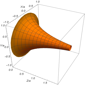
Figure 1: The core of the defect embedded in 3-dimensional Euclidean space with the coordinates $(X,Y,Z)$.

For $r>0$ the geometry given by (2.1) is conformally flat. That can be seen by introducing the Poincaré coordinate $w$ defined by $w=ae^{y/a}$. With this coordinate, the line element is written in explicitly conformally flat form

$$ds^{2}=g_{\mu\nu}dx^{\mu}dx^{\nu}=\left(\frac{a}{w}\right)^{2}\left(dt^{2}-dr^{2}-r^{2}d\phi^{2}-dw^{2}-dz^{2}\right)\ ,$$ (2.3)

where $w\in[0,\ \infty)$. The limiting values $w=0$ and $w=\infty$ correspond to the AdS boundary and horizon, respectively. In what follows we will work in the coordinate system $x^{\mu}=(t,r,\phi,w,z)$ with the metric tensor $g_{\mu\nu}=(a/w)^{2}\mathrm{diag}(1,-1,-r^{2},-1,-1)$.

We are interested in the influence of cosmic string and compactification on the properties of the ground state for a fermionic field. In the irreducible representation of the Clifford algebra the latter is presented by a 4-component spinor. In odd number of spacetime dimensions there are two inequivalent irreducible representations. In (1+4)-dimensional spacetime the corresponding set of flat spacetime Dirac matrices $\gamma_{(s)}^{(b)}$, $b=0,1,2,3,4$, can be constructed by adding to the set of the matrices $\{\gamma^{(0)},\gamma^{(1)},\gamma^{(2)},\gamma^{(3)}\}$ in (1+3)-dimensional spacetime the matrix $s\gamma^{(4)}=-s\gamma^{(0)}\gamma^{(1)}\gamma^{(2)}\gamma^{(3)}$. Here, $s=\pm 1$ distinguish two inequivalent irreducible representations. Let us denote by $\psi_{(s)}$ the 4-component field that realizes the irreducible representation with a given $s$. The corresponding Lagrangian density reads

$$L_{(s)}=\bar{\psi}_{(s)}\left[i\gamma_{(s)}^{\mu}\left(\partial_{\mu}+\Gamma_{\mu}^{(s)}+ieA_{\mu}\right)-m\right]\psi_{(s)},$$ (2.4)

where $\bar{\psi}_{(s)}=\psi_{(s)}^{\dagger}\gamma^{(0)}$ is the Dirac adjoint, $\Gamma_{\mu}^{(s)}$ is the spin connection, and $A_{\mu}$ is the vector potential for an external gauge field. The curved spacetime Dirac matrices are expressed in terms of the matrices $\gamma_{(s)}^{(b)}$ as $\gamma_{(s)}^{\mu}=e_{(b)}^{\mu}\gamma_{(s)}^{(b)}$ with vielbein fields $e_{(b)}^{\mu}$. Here and below, the tensorial indices $\mu=0,1,2,3,4$ correspond to the coordinates $(t,r,\phi,w,z)$, respectively.

For the matrices $\gamma_{(s)}^{\mu}$, $\mu=0,4$, we take $\gamma_{(s)}^{\mu}=(w/a)\delta_{b}^{\mu}\gamma_{(s)}^{(b)}$ with

$$\gamma^{(0)}=\left({\begin{array}[]{cc}0&-i\\ i&0\end{array}}\right)\ ,\;\gamma_{(+1)}^{(4)}=-\gamma_{(-1)}^{(4)}=\gamma^{(4)}=\left({\begin{array}[]{cc}0&i\\ i&0\end{array}}\right).$$ (2.5)

For the construction of the remaining matrices we use the 3D flat space $2\times 2$ Pauli matrices $\sigma^{1}$, $\sigma^{2}$, $\sigma^{3}$ in the cylindrical coordinate system $(r,\phi,w)$:

$$\sigma^{l}=\left(\frac{i}{r}\right)^{l-1}\left({\begin{array}[]{cc}0&(-1)^{l-1}e^{-iq\phi}\\ e^{iq\phi}&0\end{array}}\right)\ ,$$ (2.6)

for $l=1,2$ and $\sigma^{3}=\mathrm{diag}(1,-1)$. Here and in what follows we use the notation $q=2\pi/\phi_{0}$. In terms of those matrices we take [44]

$$\gamma_{(s)}^{l}=-i(w/a)\mathrm{diag}(\sigma^{l},-\sigma^{l}),\;l=1,2,3.$$ (2.7)

Below, the simplified notations $\gamma^{\mu}\equiv\gamma_{(+1)}^{\mu}$ and $\Gamma_{\mu}=\Gamma_{\mu}^{(+1)}$ will be used. The product $\gamma_{(s)}^{\mu}\Gamma_{\mu}^{(s)}$ in the Lagrangian density (2.4) is presented as $\gamma_{(s)}^{\mu}\Gamma_{\mu}^{(s)}=-2\gamma^{3}/w+(1-q)\gamma^{1}/(2r)$ and it is the same for both the representations.

The investigation of the FC for the fields with $s=+1$ and $s=-1$ can be unified by passing to a new representation $\psi_{(s)}^{\prime}$ with $\psi_{(+1)}^{\prime}=\psi_{(+1)}$ and $\psi_{(-1)}^{\prime}=-\gamma^{(4)}\psi_{(-1)}$, where the $\gamma^{(4)}$ matrix is given by (2.5). By using the relations $\gamma^{(4)}\gamma_{(-1)}^{\mu}\gamma^{(4)}=\gamma^{\mu}$ and $\gamma^{(4)}\gamma_{(s)}^{\mu}\Gamma_{\mu}^{(s)}\gamma^{(4)}=\gamma^{\mu}\Gamma_{\mu}$, the Lagrangian density for the new fields is presented as

$$L_{(s)}=\bar{\psi}_{(s)}^{\prime}\left[i\gamma^{\mu}\left(\partial_{\mu}+\Gamma_{\mu}+ieA_{\mu}\right)-sm\right]\psi_{(s)}^{\prime},$$ (2.8)

and differs by the sign of the mass term for two irreducible representations. The investigation described below will be presented in the representation (2.8) and the final result will be translated for the initial fields $\psi_{(s)}$.

The equation of motion corresponding to the Lagrangian density (2.8) (omitting the prime and the index $(s)$) reads

$$i\gamma^{\mu}\left(\partial_{\mu}+\Gamma_{\mu}+ieA_{\mu}\right)\psi-sm\psi=0\,.$$ (2.9)

The coordinate $z$ is compactified and in addition to the field equation one needs to specify the periodicity condition on the field operator along that direction. We will consider the quasi-periodicity condition

$$\psi(t,r,\phi,w,z+L)=e^{2\pi i\beta}\psi(t,r,\phi,w,z),$$ (2.10)

with a constant parameter $\beta$ determining the change in the phase of the transformed field. The special cases of untwisted and twisted fermionic fields correspond to $\beta=0$ and $\beta=1/2$, respectively.

In this paper, we will consider a simple configuration of the gauge field with the vector potential $A_{\mu}=(0,0,A_{2},0,A_{4})$ with constant covariant components $A_{2}$ and $A_{4}$. The component $A_{2}$ is expressed in terms of the magnetic flux $\Phi_{\mathrm{s}}$ running along the string’s core as $A_{2}=-q\Phi_{\mathrm{s}}/(2\pi)$. We can also introduce a magnetic flux $\Phi_{\mathrm{c}}$ related to the component $A_{4}$ as $A_{4}=-\Phi_{\mathrm{c}}/L$. Formally, the latter can be interpreted as a magnetic flux enclosed by the compact dimension. It gets a real physical meaning in the braneworld realization of the model, where the setup under consideration is embedded in a (1+5)-dimensional spacetime as a fermionic field localized on a hypersurface (brane).

We are interested in the influence of the gravitational field and of nontrivial spatial topology on the local properties of the fermionic vacuum. As important local characteristic the FC will be considered. Another local characteristic, the VEV of the current density, has been investigated in a recent publication [44]. The VEV of a physical observable bilinear in the field operator is expressed in terms of the mode sum over a complete set of solutions of the field equation. This set of solutions for the problem under consideration is given in [44] and we will describe it to fix the notations and for the further use in the evaluation of the FC.

In accordance with the problem symmetry, the dependence of the positive and negative energy spinorial modes on the coordinates $t$ and $z$ can be taken in the form $e^{ik_{z}z\mp iEt}$, where $E>0$. Decomposing the $4$-component spinor $\psi$ into the upper and lower $2$-component ones, from the Dirac equation (2.9) a second order differential equation is obtained for each component. Separating the variables it can be seen the dependence on the coordinates $r$ and $w$ is expressed in terms of cylinder functions. Additional conditions relating two components of the spinor are imposed in order to uniquely specify the wave-functions [47]. Denoting by $\sigma$ the complete set of quantum numbers specifying the solutions, the positive and negative energy mode functions are presented as

$$\psi_{\sigma}^{(\pm)}(x)=C_{\sigma}^{(\pm)}w^{5/2}\left({\begin{array}[]{c}J_{\beta_{j}}(\lambda r)J_{\nu_{1}}(pw)e^{-iq\phi/2}\\ \mp s\epsilon_{j}\kappa_{\eta}b_{\eta}^{(\pm)}J_{\beta_{j}+\epsilon_{j}}(\lambda r)J_{\nu_{2}}(pw)e^{iq\phi/2}\\ is\kappa_{\eta}J_{\beta_{j}}(\lambda r)J_{\nu_{2}}(pw)e^{-iq\phi/2}\\ \pm i\epsilon_{j}b_{\eta}^{(\pm)}J_{\beta_{j}+\epsilon_{j}}(\lambda r)J_{\nu_{1}}(pw)e^{iq\phi/2}\end{array}}\right)e^{iqj\phi+ik_{z}z\mp iEt}\ ,$$ (2.11)

where $0\leq\lambda,p<\ \infty$, $j=\pm 1/2,\pm 3/2,...$, and $J_{\nu}(x)$ is the Bessel function. The eigenvalues of the momentum $k_{z}$ along the axis $z$ are determined by the quasiperiodicity condition (2.10) and are given by $k_{z}=k_{l}=2\pi(l+\beta)/L$, where $l=0,\pm 1,\pm 2,...$. The energy $E$ is expressed in terms of the quantum numbers by the relation

$$E=\sqrt{\lambda^{2}+p^{2}+\tilde{k}_{l}^{2}}\,\ ,$$ (2.12)

where

$$\tilde{k}_{l}=2\pi(l+\tilde{\beta})/L,\;\tilde{\beta}=\beta-\Phi_{\mathrm{c}}/\Phi_{0},$$ (2.13)

being $\Phi_{0}=2\pi/e$ the magnetic flux quantum. The notations appearing in the orders of the Bessel functions are given by

$$\beta_{j}=q|j+\alpha|-\epsilon_{j}/2\ ,\ \ \nu_{l}=ma+(-1)^{l}s/2\ ,$$ (2.14)

where $\alpha=eA_{2}/q=-\Phi_{\mathrm{s}}/\Phi_{0}$ and $\epsilon_{j}=1$ for $j>-\alpha$ and $\epsilon_{j}=-1$ for $j<-\alpha$. The coefficients $\kappa_{\eta}$ and $b_{\eta}^{(\pm)}$, with $\eta=-1,+1$, are defined by the relations

$$\kappa_{\eta}=\frac{1}{p}\left(-\tilde{k}_{l}+\eta\sqrt{\tilde{k}_{l}^{2}+p^{2}}\right),$$

$$b_{\eta}^{(\pm)}=\frac{1}{\lambda}\left(E\mp\eta\sqrt{\tilde{k}_{l}^{2}+p^{2}}\right)\ .$$ (2.15)

The normalization coefficient is given by the expression

$$|C_{\sigma}^{(\pm)}|^{2}=\frac{\eta qp^{2}\lambda^{2}}{8\pi a^{4}LE\kappa_{\eta}b_{\eta}^{(\pm)}\sqrt{\tilde{k}_{l}^{2}+p^{2}}}\ .$$ (2.16)

The complete set of quantum numbers $\sigma$ is specified as $\sigma=(\lambda,p,j,l,\eta)$. Note that the mode functions (2.11) are the eigenfunctions of the projection of the total angular momentum on the $w$-axis with the eigenvalues $qj$:

$$\hat{J}_{3}\psi_{\sigma}^{(\pm)}(x)=\left(-i\partial_{\phi}+q\Sigma^{3}/2\right)\psi_{\sigma}^{(\pm)}(x)=qj\psi_{\sigma}^{(\pm)}(x)\ ,$$ (2.17)

where $\Sigma^{3}=\mathrm{diag}(\sigma^{3},\sigma^{3})$.

In the discussion above we have used the coordinates $(t,r,\phi,w,z)$. The corresponding coordinates in pure AdS spacetime with $-\infty<z<+\infty$ are referred to as Poincaré coordinates. Our choice of those coordinates is motivated by the fact that the braneworld models and the discussions of AdS/CFT correspondence employ the Poincaré patch. With $0<w<+\infty$, the Poincaré coordinates cover a half of global AdS spacetime. The second half is covered by the coordinates $(t,r,\phi,w,z)$ with $-\infty<w<0$. The mode functions corresponding to that patch are obtained from (2.11) by an analytic continuation. The latter is reduced to the analytic continuation of the Bessel functions with the arguments $pw$. In a similar way, the expressions for the FC in the second Poincaré patch are obtained by  a simple analytic continuation from the region $w>0$ to the region $w<0$. In both Poincaré and global coordinates time-like Killing vectors are present and we can define the corresponding vacuum states. It is important to note that the Poincaré and global vacuum states are equivalent (see, for example, [48, 49]).

3 Fermionic condensate in the uncompactified geometry

The FC is defined as the VEV $\langle 0|\bar{\psi}\psi|0\rangle\equiv\langle\bar{\psi}\psi\rangle$, where $|0\rangle$ is the vacuum state (Poincaré vacuum) and $\bar{\psi}=\psi^{\dagger}\gamma^{(0)}$ is the Dirac adjoint. Note that in the definition of the Dirac adjoint $\gamma^{(0)}$ is the flat spacetime matrix (2.5). We start our investigation first considering the geometry where the $z$-direction is not compactified, $-\infty<z<+\infty$. The fermionic vacuum polarization in the geometry of a straight cosmic string on the Minkowski bulk has been investigated in [50]-[53]. The effects induced by the presence of additional boundaries were discussed in [54, 55]. The FC and the expectation values of the current density and energy-momentum tensor in (1+2)-dimensional conical spacetime with circular boundaries have been considered in [56]-[61].

In the geometry with uncompactified $z$-direction the corresponding fermionic mode functions are given by (2.11) where now the momentum along the $z$-direction is continuous, $-\infty<k_{z}<+\infty$, and in the relations (2.12)-(2.16) the replacement $\tilde{k}_{l}\rightarrow k_{z}$ should be made. In addition, in the normalization coefficient (2.16) one needs to replace $L$ by $2\pi$. Expanding the field operator in terms of the complete set $\{\psi_{\sigma}^{(-)},\psi_{\sigma}^{(+)}\}$, and using the anticommutation relations for the creation and annihilation operators, for the FC the following mode sum formula is obtained:

$$\langle\bar{\psi}\psi\rangle=-\frac{1}{2}\sum_{\sigma}\sum_{\chi=-,+}\chi\bar{\psi}_{\sigma}^{(\chi)}\psi_{\sigma}^{(\chi)},$$ (3.1)

where the summation goes over the set of quantum numbers as

$$\sum_{\sigma}=\sum_{j}\int_{0}^{\infty}d\lambda\int_{0}^{\infty}dp\int_{-\infty}^{\infty}dk_{z}\sum_{\eta=\pm 1}\ .$$ (3.2)

Here and in what follows $\sum_{j}=\sum_{j=\pm 1/2,\pm 3/2,\cdots}$. The operators in the definition of the FC are given at the same spacetime point and the expression in the right-hand side of (3.1) is divergent. Various regularization schemes can be employed to make the expression finite. For example, we can use the point-splitting technique or a cutoff function can be introduced. The details of the evaluation procedure described below do not depend on the specific regularization method.

Substituting the mode functions in (3.1), for the FC in the uncompactified geometry we obtain

$$\langle\bar{\psi}\psi\rangle_{\mathrm{cs}}^{\mathrm{AdS}}=-\frac{sqw^{5}}{16\pi^{2}a^{4}}\sum_{\sigma}\sum_{\chi=-,+}\frac{\chi\eta p^{2}\lambda^{2}}{E\sqrt{p^{2}+k_{z}^{2}}}J_{\nu_{1}}(pw)J_{\nu_{2}}(pw)\left[b_{\eta}^{(-\chi)}J_{\beta_{j}}^{2}(\lambda r)-b_{\eta}^{(\chi)}J_{\beta_{j}+\epsilon_{j}}^{2}(\lambda r)\right],$$ (3.3)

where the property $b_{\eta}^{(+)}b_{\eta}^{(-)}=1$ has been used. By taking into account the expression for $b_{\eta}^{(\pm)}$ and summing over $\eta$, this formula is simplified to

$$\langle\bar{\psi}\psi\rangle_{\mathrm{cs}}^{\mathrm{AdS}} = -\frac{sqw^{5}}{4\pi^{2}a^{4}}\sum_{j}\int_{0}^{\infty}d\lambda\int_{0}^{\infty}dp\int_{-\infty}^{\infty}dk_{z}\frac{\lambda p^{2}}{\sqrt{\lambda^{2}+p^{2}+k_{z}^{2}}}$$ (3.4)

$$\times J_{\nu_{1}}(pw)J_{\nu_{2}}(pw)\left[J_{\beta_{j}}^{2}(\lambda r)+J_{\beta_{j}+\epsilon_{j}}^{2}(\lambda r)\right]\ .$$

From here it follows that the FC has opposite signs for the fields with $s=+1$ and $s=-1$. So, in this section we will consider the case $s=+1$ and, hence, in the corresponding expressions $\nu_{1}=ma-1/2$ and $\nu_{2}=ma+1/2$.

For the further transformation of the expression (3.4), we use the identity

$$\frac{1}{\sqrt{\lambda^{2}+p^{2}+k_{z}^{2}}}=\frac{2}{\sqrt{\pi}}\int_{0}^{\infty}d\tau e^{-\tau^{2}(\lambda^{2}+p^{2}+k_{z}^{2})}\ .$$ (3.5)

Plugging this in (3.4) the integrals over the quantum numbers $\lambda$, $p$ and $k_{z}$ are evaluated by using the results from [62]. After some intermediate steps, introducing instead of $\tau$ a new integration variable $y=r^{2}/2\tau^{2}$, we get

$$\langle\bar{\psi}\psi\rangle_{\mathrm{cs}}^{\mathrm{AdS}} = -\frac{q(w/r)^{6}}{4\pi^{2}a^{4}}\int_{0}^{\infty}dx\,x^{2}e^{-(1+\rho^{-2})x}\left[I_{\nu_{1}}\left(x/\rho^{2}\right)-I_{\nu_{2}}\left(x/\rho^{2}\right)\right]$$ (3.6)

$$\times\sum_{j}\left[I_{\beta_{j}}\left(x\right)+I_{\beta_{j}+\epsilon_{j}}\left(x\right)\right]\ ,$$

where $I_{\nu}(z)$ represents the modified Bessel function [63]. In (3.6),

$$\rho=r/w$$ (3.7)

is the proper distance from the string, $r_{p}=ar/w$, measured in units of $a$.

At this point it is convenient to decompose the parameter $\alpha$ as

$$\alpha=\alpha_{0}+n_{0}\ ,\quad|\alpha_{0}|<1/2\ ,$$ (3.8)

where $n_{0}$ is an integer. Note that if we shift $j+n_{0}\rightarrow j$, the VEV (3.6) remains unchanged, which implies that it does not depend on the integer part $n_{0}$. An integral representation for the part

$${\mathcal{J}}(q,\alpha_{0},x)=\sum_{j}\left[I_{\beta_{j}}\left(x\right)+I_{\beta_{j}+\epsilon_{j}}\left(x\right)\right]$$ (3.9)

is found by using the representation for the series $\sum_{j}I_{\beta_{j}}(x)$ given in [56]. The representation reads

$${\mathcal{J}}(q,\alpha_{0},x) = \frac{2}{q}e^{x}+\frac{4}{\pi}\int_{0}^{\infty}du\frac{h(q,\alpha_{0},2u)\sinh u}{\cosh(2qu)-\cos(q\pi)}e^{-x\cosh 2u}$$ (3.10)

$$+\frac{4}{q}\sideset{}{{}^{\prime}}{\sum}_{k=1}^{[q/2]}(-1)^{k}\cos(\pi k/q)\cos(2\pi k\alpha_{0})e^{x\cos(2\pi k/q)}\ ,$$

where $[q/2]$ stands for the integer part of $q/2$ and

$$h(q,\alpha_{0},x) = \cos[\pi q(1/2+\alpha_{0})]\sinh[(1/2-\alpha_{0})qx]$$ (3.11)

$$+\cos[\pi q(1/2-\alpha_{0})]\sinh[(1/2+\alpha_{0})qx]\ .$$

The prime on the summation sign over $k$ means that for even values of $q$ the term with $k=q/2$ should be halved. In the case $1\leqslant q<2$, the last term on the right-hand side of (3.10) must be omitted. Note that $h(q,\alpha_{0},z)$ and ${\mathcal{J}}(q,\alpha_{0},y)$ are even functions of $\alpha_{0}$.

Introducing a new integration variable, the contribution to the condensate (3.6) coming from the term with $e^{x}$ in (3.10) is presented as

$$\langle\bar{\psi}\psi\rangle^{\mathrm{AdS}}=-\frac{1}{2\pi^{2}a^{4}}\int_{0}^{\infty}dx\,x^{2}e^{-x}\left[I_{\nu_{1}}\left(x\right)-I_{\nu_{2}}\left(x\right)\right].$$ (3.12)

It does not depend on $q$ and $\alpha_{0}$ and corresponds to th FC in (1+4)-dimensional AdS spacetime in the absence of cosmic string. As we could expect from the maximal symmetry of the AdS spacetime the latter does not depend on spacetime point. It is of interest to compare the FC (3.12) with the condensate in de Sitter (dS) spacetime. The latter has been investigated in [64] for the Bunch-Davies vacuum state in general number of spatial dimensions. Specified to the case of (1+4)-dimensional dS spacetime with the curvature radius $a$, the unregularized FC is expressed as

$$\langle\bar{\psi}\psi\rangle^{\mathrm{dS}}=\frac{1}{\pi^{3}a^{4}}\int_{0}^{\infty}dx\,x^{2}e^{x}\mathrm{Im}\left[K_{1/2-ima}\left(x\right)\right],$$ (3.13)

where $K_{\nu}(x)$ is the Macdonald function. The expressions in the right-hand sides of (3.12) and (3.13) are divergent and need a regularization with further renormalization. For the regularization of (3.13) in [64] a cutoff function is introduced. The renormalization ambiguity is fixed by an additional condition, requiring $\lim_{m\rightarrow\infty}\langle\bar{\psi}\psi\rangle^{\mathrm{dS}}=0$. The renormalized condensate $\langle\bar{\psi}\psi\rangle_{\mathrm{ren}}^{\mathrm{dS}}$ is negative in spatial dimensions 3,5,6 and positive in 4-dimensional space. The renormalization of the condensate (3.12) is done in a way similar to that used in [64]. We will address that point elsewhere.

In the present paper we are interested in the effects induced by cosmic string. The corresponding contribution to the FC is given by

$$\langle\bar{\psi}\psi\rangle_{\mathrm{cs}}=\langle\bar{\psi}\psi\rangle_{\mathrm{cs}}^{\mathrm{AdS}}-\langle\bar{\psi}\psi\rangle^{\mathrm{AdS}}.$$ (3.14)

An important point to mention here is that for $r>0$ the difference (3.14) is finite and the regularization implicitly assumed before can be safely removed. The physical reason of the absence of divergences in $\langle\bar{\psi}\psi\rangle_{\mathrm{cs}}$ is that the local geometry in the region $r>0$ is not changed by the cosmic string and, hence, new divergences will not arise. Substituting (3.10) in (3.6) we get

$$\langle\bar{\psi}\psi\rangle_{\mathrm{cs}} = -\frac{1}{\pi^{2}a^{4}}\int_{0}^{\infty}dx\,x^{2}e^{-x}\left[I_{\nu_{1}}\left(x\right)-I_{\nu_{2}}\left(x\right)\right]$$ (3.15)

$$\times\Biggl{\{}\sideset{}{{}^{\prime}}{\sum}_{k=1}^{[q/2]}(-1)^{k}\cos(\pi k/q)\cos(2\pi k\alpha_{0})e^{-2x\rho^{2}\sin^{2}(\pi k/q)}$$

$$+\frac{q}{\pi}\int_{0}^{\infty}du\frac{h(q,\alpha_{0},2u)\sinh u}{\cosh(2qu)-\cos(q\pi)}e^{-2x\rho^{2}\cosh^{2}u}\Biggr{\}}\ .$$

The integral over $x$ is valuated by using the integration formula from [62]:

$$\int_{0}^{\infty}dx\,x^{\mu-1}e^{-ux}I_{\nu}(x)=\sqrt{\frac{2}{\pi}}\frac{e^{-(\mu-1/2)\pi i}Q_{\nu-1/2}^{\mu-1/2}(u)}{(u^{2}-1)^{\mu/2-1/4}}\ ,$$ (3.16)

where $u>1$ and $Q_{\nu}^{\mu}(z)$ represents the associated Legendre function [63]. After some intermediate steps, the expression for the FC induced by the cosmic string reads

$$\langle\bar{\psi}\psi\rangle_{\mathrm{cs}} = -\frac{\sqrt{2}}{\pi^{5/2}a^{4}}\Biggl{[}\sideset{}{{}^{\prime}}{\sum}_{k=1}^{[q/2]}(-1)^{k}\cos(\pi k/q)\cos(2\pi k\alpha_{0}){\mathcal{Z}}_{ma}(u_{k})$$ (3.17)

$$+\frac{q}{\pi}\int_{0}^{\infty}dx\frac{h(q,\alpha_{0},2x)\sinh x}{\cosh(2qx)-\cos(q\pi)}{\mathcal{Z}}_{ma}(u_{x})\Biggr{]}\ .$$

Here we have introduced the notation

$${\mathcal{Z}}_{ma}(u)=F_{\nu_{1}}(u)-F_{\nu_{2}}(u)\,,$$ (3.18)

with the function

$$F_{\nu}(u)=\frac{e^{-i5\pi/2}Q_{\nu-1/2}^{5/2}(u)}{(u^{2}-1)^{5/4}}\,,$$ (3.19)

and the variables

$$u_{k} = 1+2\rho^{2}\sin^{2}(\pi k/q)\ ,$$

$$u_{x} = 1+2\rho^{2}\cosh^{2}x\ .$$ (3.20)

Note that the FC $\langle\bar{\psi}\psi\rangle_{\mathrm{cs}}$ depends on the coordinates $r$ and $w$ through the ratio (3.7). This property is a consequence of the maximal symmetry of the AdS spacetime.

For a massless field, the function ${\mathcal{Z}}_{ma}(u)$ is expressed in terms of elementary functions:

$${\mathcal{Z}}_{0}(u)=\frac{3\sqrt{\pi}}{4(1+u)^{5/2}}\ .$$ (3.21)

Taking this expression into (3.17), we get

$$\langle\bar{\psi}\psi\rangle_{\mathrm{cs}} = -\frac{3}{16\pi^{2}a^{4}}\Biggl{[}\sideset{}{{}^{\prime}}{\sum}_{k=1}^{[q/2]}(-1)^{k}\frac{\cos(\pi k/q)\cos(2\pi k\alpha_{0})}{(1+\rho^{2}\sin^{2}(\pi k/q))^{5/2}}$$ (3.22)

$$+\frac{q}{\pi}\int_{0}^{\infty}dx\frac{\sinh x}{\cosh(2qx)-\cos(q\pi)}\frac{h(q,\alpha_{0},2x)}{(1+\rho^{2}\cosh^{2}x)^{5/2}}\Biggr{]}\ .$$

Near the string, $\rho\ll 1$, and for

$$2|\alpha_{0}|<1-1/q\,,$$ (3.23)

the leading term in the expansion of the FC (3.22) is obtained directly putting $\rho=0$. In this case the FC is finite on the string and

$$\langle\bar{\psi}\psi\rangle_{\mathrm{cs}}|_{r=0}=-\frac{3h_{0}(q,\alpha_{0})}{16\pi^{2}a^{4}}.$$ (3.24)

Here and in what follows the notation

$$h_{n}(q,\alpha_{0})=\sideset{}{{}^{\prime}}{\sum}_{k=1}^{[q/2]}\frac{(-1)^{k}\cos(\pi k/q)}{\sin^{n}(\pi k/q)}\cos(2\pi k\alpha_{0})+\frac{q}{\pi}\int_{0}^{\infty}dx\,\frac{h(q,\alpha_{0},2x)\sinh x}{\left[\cosh(2qx)-\cos(q\pi)\right]\cosh^{n}x}\ ,$$ (3.25)

is introduced. For

$$2|\alpha_{0}|>1-1/q\,,$$ (3.26)

the dominant contribution to the FC (3.22) comes from the integral term. In this case we cannot directly put $\rho=0$ because the integral diverges at the lower limit. It can be seen that the dominant contribution to the integral comes from the integration range $x\sim\ln(1/\rho)$. On the base of this we can show that, to the leading order,

$$\langle\bar{\psi}\psi\rangle_{\mathrm{cs}}\approx-\frac{q\cos[\pi q(1/2-|\alpha_{0}|)]}{16\pi^{7/2}a^{4}\left(\rho/2\right)^{1+\left(2|\alpha_{0}|-1\right)q}}\Gamma\left(2+\left(1/2-|\alpha_{0}|\right)q\right)\Gamma\left(1/2-\left(1/2-|\alpha_{0}|\right)q\right),$$ (3.27)

and the condensate (3.22) diverges on the string like $1/\rho^{1+\left(2|\alpha_{0}|-1\right)q}$. Note that under the condition (3.26) the leading term (3.27) is negative.

Another special case corresponds to a magnetic flux in the absence of planar angle deficit with $q=1$. Denoting by $\langle\bar{\psi}\psi\rangle_{\mathrm{mf}}=\langle\bar{\psi}\psi\rangle_{\mathrm{cs}}|_{q=1}$ the part in the FC induced by the magnetic flux, from (3.17) we obtain

$$\langle\bar{\psi}\psi\rangle_{\mathrm{mf}}=-\frac{\sqrt{2}\sin(\pi\alpha_{0})}{\pi^{7/2}a^{4}}\int_{0}^{\infty}dx\sinh(2\alpha_{0}x)\tanh(x){\mathcal{Z}}_{ma}(1+2\rho^{2}\cosh^{2}x).\$$ (3.28)

The expression for the function (3.25), specified for this case, takes the form

$$h_{n}(1,\alpha_{0})=\frac{1}{\pi}\sin(\pi\alpha_{0})\int_{0}^{\infty}dx\,\frac{\sinh(2\alpha_{0}x)}{\cosh^{n+1}x}\sinh x\ .$$ (3.29)

This expression should be used in the asymptotic estimates below for the magnetic flux-induced contribution in the FC when the planar angle deficit is absent.

Now, let us return to the general case of the parameter $q$ and analyse some asymptotic properties of the FC induced by the cosmic string. In the Minkowskian limit, we have $a\rightarrow\infty$ with $y$ fixed. This implies in $w\approx a+y$ and $ma\gg 1$. In this limit one needs the asymptotic behavior of the function $Q_{\nu-1/2}^{5/2}(u)$ for $u-1\ll 1$ and $\nu\gg 1$. In the literature we could find only the leading term in the corresponding asymptotic expansion. The leading term is cancelled in the corresponding expansion of the function ${\mathcal{Z}}_{ma}(u)$ and the next-to-leading order term is required. In our calculation we have used the representation (3.6) with the function ${\mathcal{J}}(q,\alpha_{0},y)$ from (3.10). By using the uniform asymptotic expansion for the function $I_{\nu}(x)$ for large values of the order it can be seen that in the limit $a\rightarrow\infty$, to the leading order, one finds

$$\int_{0}^{\infty}dxx^{2}e^{-\left(1+2b^{2}/w^{2}\right)x}\left[I_{ma-1/2}(x)-I_{ma+1/2}(x)\right]\approx\sqrt{\frac{2}{\pi}}a^{4}m^{4}f_{3/2}\left(2mb\right),$$ (3.30)

with the notation $f_{\nu}(x)=K_{\nu}(x)/x^{\nu}$, being $K_{\nu}(x)$ the Macdonald function [63]. For the FC induced by cosmic string in (1+4)-dimensional Minkowski spacetime this gives

$$\langle\bar{\psi}\psi\rangle_{\mathrm{cs}}^{\mathrm{(M)}} = -\frac{\sqrt{2}m^{4}}{\pi^{5/2}}\left[\frac{q}{\pi}\int_{0}^{\infty}dx\frac{h(q,\alpha_{0},2x)\sinh x}{\cosh(2qx)-\cos(q\pi)}f_{3/2}\left(2mr\cosh x\right)\right.$$ (3.31)

$$\left.+\sideset{}{{}^{\prime}}{\sum}_{k=1}^{[q/2]}(-1)^{k}\cos(\pi k/q)\cos(2\pi k\alpha_{0})f_{3/2}\left(2mr\sin(\pi k/q)\right)\right].$$

Note that the function $f_{3/2}\left(x\right)$ is expressed in terms of elementary functions:

$$f_{3/2}\left(x\right)=\sqrt{\frac{\pi}{2}}\frac{x+1}{x^{3}}e^{-x}.$$ (3.32)

For a massless field the condensate (3.31) vanishes. This result is also seen from (3.22) taking the limit $a\rightarrow\infty$ with fixed $y$. Hence, the generation of the FC for a massless field is purely gravitational effect.

At small proper distances from the string compared with the curvature radius we have $\rho\ll 1$ and for a massive field one gets

$$\langle\bar{\psi}\psi\rangle_{\mathrm{cs}}\approx-\frac{mh_{3}(q,\alpha_{0})}{8\pi^{2}(ar/w)^{3}}\ .$$ (3.33)

As seen, in this case the FC diverges on the string like $1/r_{p}^{3}$. The leading term (3.33) coincides with that for the string in the Minkowski bulk, given by (3.31), replacing the Minkowskian distance $r$ by the proper distance $r_{p}=ar/w$ in the AdS bulk. This shows that for a massive field the effects of gravity near the string are weak. At large distances from the string’s core, $\rho\gg 1$, with $w$ fixed, we use the asymptotic

$${\mathcal{Z}}_{ma}(u)\approx\frac{\sqrt{\pi}(ma+1/2)(ma+3/2)}{2^{ma}u^{ma+5/2}}\ ,$$ (3.34)

for $u\gg 1$. Pluging this into (3.17), to the leading order, we obtain

$$\langle\bar{\psi}\psi\rangle_{\mathrm{cs}}\approx-\frac{\left(ma+1/2\right)(ma+3/2)}{2^{2ma+2}\pi^{2}a^{4}(r/w)^{2ma+5}}h_{2ma+5}(q,\alpha_{0})\ .$$ (3.35)

For a massless field this result could also be directly obtained from (3.22). We see that the decay of the FC at large distance from the string is power-law for both massless and massive fields. Note that, as it is seen from (3.31), in the Minkowski bulk at large distances, $mr\gg 1$, the FC decays exponentially.

By taking into account that the FC depends on the coordinates $r$ and $w$ in the form of the ratio $r/w$, from the asymptotic expressions given above for $\rho\ll 1$ and $\rho\gg 1$ we can obtain the behavior of the condensate near the AdS boundary and horizon. For points near the boundary, assuming that $w\ll r$, the leading term in the corresponding asymptotic expansion is given by (3.35) and the condensate $\langle\bar{\psi}\psi\rangle_{\mathrm{cs}}$ vanishes on the AdS boundary as $w^{2ma+5}$. Near the horizon one has $w\gg r$ and for a massive field, in accordance with (3.33), the contribution of the cosmic string in the FC diverges on the horizon like $w^{3}$. For a massless field and under the condition (3.26) the divergence is weaker, $\langle\bar{\psi}\psi\rangle_{\mathrm{cs}}\propto w^{1+\left(2|\alpha_{0}|-1\right)q}$. In the range of parameters $2|\alpha_{0}|<1-1/q$ the condensate $\langle\bar{\psi}\psi\rangle_{\mathrm{cs}}$ is finite on the horizon with the limiting value given by the right-hand side of (3.24).

In Fig. 2 we have plotted the FC in the geometry where the $z$-direction is not compactified as a function of the ratio $r/w$. The latter is the proper distance from the string in units of the curvature radius $a$, measured by an observer with the coordinate $w$. The graphs are plotted for $\alpha_{0}=0.3$ and the numbers near the curves are the values of the parameter $q$. The left panel corresponds to a massive fermionic field with $ma=1$ and the right panel presents the results for a massless field. As it has been already clarified by the asymptotic analysis, for a massive field the condensate $\langle\bar{\psi}\psi\rangle_{\mathrm{cs}}$ diverges on the string like $(w/r)^{3}$. For a massless field, $\langle\bar{\psi}\psi\rangle_{\mathrm{cs}}$ diverges as $\left(w/r\right)^{1+\left(2|\alpha_{0}|-1\right)q}$ under the condition (3.26) (the curves with $q=1,2$ on the right panel) and takes finite value (3.24) on the string under the condition (3.23) (the curve $q=3$ on the right panel). Note that for the case $q=3$ on the right panel $\langle\bar{\psi}\psi\rangle_{\mathrm{cs}}|_{r=0}\approx 0.0095/a^{4}$.

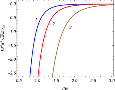
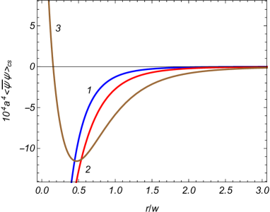
Figure 2: The FC $\langle\bar{\psi}\psi\rangle_{\mathrm{cs}}$ as a function of the distance from the string for massive (left panel) and massless (right panel) fields. The graphs are plotted for $\alpha_{0}=0.3$ and for different values of $q$ (numbers near the curves). On the left panel we have taken $ma=1$.

The left panel of Fig. 3 presents the dependence of the FC $\langle\bar{\psi}\psi\rangle_{\mathrm{cs}}$ on the mass of the field, in units of $1/a$, for $r/w=1.5$ and $\alpha_{0}=0.3$. The right panel in Fig. 3 displays the dependence of the FC $\langle\bar{\psi}\psi\rangle_{\mathrm{cs}}$ on $\alpha_{0}$ for fixed values of $ma=0.5$ and $r/w=1.5$. On both panels the numbers near the curves correspond to the values of the parameter $q$.

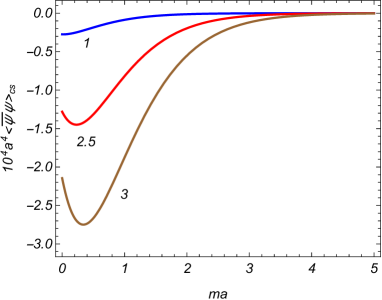
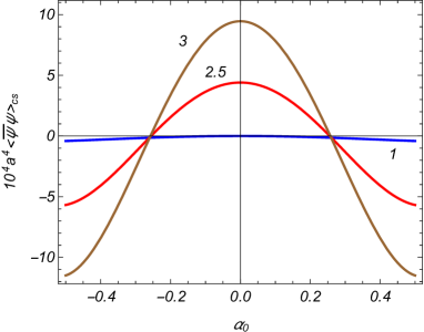
Figure 3: The condensate $\langle\bar{\psi}\psi\rangle_{\mathrm{cs}}$ as a function of the mass (left panel) and of the parameter $\alpha_{0}$ (right panel) for fixed $r/w=1.5$ and for different values of $q$ (numbers near curves). For the left panel we have taken $\alpha_{0}=0.3$ and for the right panel $ma=0.5$.

We recall that the consideration above was presented in terms of the fields $\psi_{(s)}^{\prime}$ with the Lagrangian density (2.8) and the formulas given above are for the FC $\langle\bar{\psi}_{(s)}^{\prime}\psi_{(s)}^{\prime}\rangle$ with $s=+1$. As it has been shown above

$$\langle\bar{\psi}_{(-1)}^{\prime}\psi_{(-1)}^{\prime}\rangle=-\langle\bar{\psi}_{(+1)}^{\prime}\psi_{(+1)}^{\prime}\rangle.$$ (3.36)

Having the results for $\langle\bar{\psi}_{(s)}^{\prime}\psi_{(s)}^{\prime}\rangle$ we can obtain the corresponding quantity in terms of the initial fields $\psi_{(s)}$ with the Lagrangian density (2.4). By using the relation between the fields $\psi_{(s)}$ and $\psi_{(s)}^{\prime}$ one can see that

$$\langle\bar{\psi}_{(s)}\psi_{(s)}\rangle=s\langle\bar{\psi}_{(s)}^{\prime}\psi_{(s)}^{\prime}\rangle.$$ (3.37)

From here we conclude that the FC $\langle\bar{\psi}_{(s)}\psi_{(s)}\rangle$ is the same for two irreducible representations $s=+1$ and $s=-1$. For (1+4)-dimensional spacetime the mass term in the Lagrangian density (2.4) is not invariant under the parity transformation ($P$) and charge conjugation ($C$). Invariant massive fermionic models can be constructed considering a system of two 4-component fields $\psi_{(+1)}$ and $\psi_{(-1)}$ with the Lagrangian density $L=\sum_{s=\pm 1}L_{(s)}$. In those models the total FC induced by cosmic string in the uncompactified geometry is obtained summing the separate contributions, $\sum_{s=\pm 1}\langle\bar{\psi}_{(s)}\psi_{(s)}\rangle_{\mathrm{cs}}$. These contributions coincide for the fields with $s=+1$ and $s=-1$ and are given by the expressions for $\langle\bar{\psi}\psi\rangle_{\mathrm{cs}}$ presented above.

4 Topological effects of compactification

In this section we consider the FC in the geometry with compactified $z$-direction. The scalar and fermionic vacua polarizations around a compactified cosmic string in the Minkowksi bulk have been investigated in [65, 66, 67]. The mode sum for the FC is still given by (3.1) where now the mode functions are expressed as (2.11) and the collective summation is understood as

$$\sum_{\sigma}=\int_{0}^{\infty}d\lambda\int_{0}^{\infty}dp\sum_{j}\sum_{l=-\infty}^{\infty}\sum_{\eta=\pm 1}\,.$$ (4.1)

Substituting the mode functions, in a way similar to (3.4), we find the representation

$$\langle\bar{\psi}\psi\rangle = -\frac{sqw^{5}}{2\pi a^{4}L}\int_{0}^{\infty}d\lambda\int_{0}^{\infty}dp\sum_{j}\sum_{l=-\infty}^{\infty}\frac{\lambda p^{2}}{\sqrt{\lambda^{2}+p^{2}+\tilde{k}_{l}^{2}}}$$ (4.2)

$$\times J_{\nu_{1}}(pw)J_{\nu_{2}}(pw)\left[J_{\beta_{j}}^{2}(\lambda r)+J_{\beta_{j}+\epsilon_{j}}^{2}(\lambda r)\right]\ .$$

Again, the FC has opposite signs in the cases $s=+1$ and $s=-1$ and we continue the investigation for $s=+1$ and, hence, in the discussion below $\nu_{1}=ma-1/2$, $\nu_{2}=ma+1/2$.

In order to separate the contribution in the FC induced by the compactification of the $z$-direction, for the summation over $l$ we use the Abel-Plana-type formula [68]

$$\sum_{l=-\infty}^{\infty}f(|l+\tilde{\beta}|)=2\int_{0}^{\infty}du\,f(u)+i\int_{0}^{\infty}du\sum_{n=\pm 1}\frac{f(iu)-f(-iu)}{e^{2\pi(u+in\tilde{\beta})}-1},$$ (4.3)

with the function $f(u)=[\lambda^{2}+p^{2}+(2\pi u/L)^{2}]^{-1/2}$. Comparing with (3.4), we see that the contribution to the FC coming from the first integral in (4.3) coincides with the FC in the uncompactified geometry. In this way the following decomposition is obtained:

$$\langle\bar{\psi}\psi\rangle=\langle\bar{\psi}\psi\rangle_{\mathrm{cs}}^{\mathrm{AdS}}+\langle\bar{\psi}\psi\rangle_{\mathrm{c}}\,,$$ (4.4)

where the second term in the right-hand side comes from the second integral in (4.3) and contains the effects induced by the compactification. For that contribution one gets

$$\langle\bar{\psi}\psi\rangle_{\mathrm{c}} = -\frac{qw^{5}}{2\pi^{2}a^{4}}\int_{0}^{\infty}d\lambda\,\lambda\int_{0}^{\infty}dp\,p^{2}\sum_{j}[J_{\beta_{j}}^{2}(\lambda r)+J_{\beta_{j}+\epsilon_{j}}^{2}(\lambda r)]$$ (4.5)

$$\times J_{\nu_{1}}(pw)J_{\nu_{2}}(pw)\int_{\sqrt{\lambda^{2}+p^{2}}}^{\infty}dx\sum_{n=\pm 1}\frac{\left(x^{2}-\lambda^{2}-p^{2}\right)^{-1/2}}{e^{Lx+2\pi in\tilde{\beta}}-1}\ ,$$

where a new integration variable $x=2\pi u/L$ is introduced. Note that for $r>0$ the topological part $\langle\bar{\psi}\psi\rangle_{\mathrm{c}}$ is finite and implicit regularization assumed before can be removed. The renormalization is required for the part $\langle\bar{\psi}\psi\rangle_{\mathrm{cs}}^{\mathrm{AdS}}$ only and that has been discussed in the previous section. The physical reason for the finiteness of $\langle\bar{\psi}\psi\rangle_{\mathrm{c}}$ is that the structure of divergences is completely determined by the local geometry and the latter is not changed by the compactification under consideration.

For the further transformation of the condensate $\langle\bar{\psi}\psi\rangle_{\mathrm{c}}$ we use the expansion $(e^{u}-1)^{-1}=\sum_{l=1}^{\infty}e^{-lu}$ in the integral over $x$. The integrals for a given $l$ are expressed in terms of the Macdonald function and one obtains

$$\langle\bar{\psi}\psi\rangle_{\mathrm{c}} = -\frac{qw^{5}}{\pi^{2}a^{4}}\sum_{l=1}^{\infty}\cos(2\pi l\tilde{\beta})\int_{0}^{\infty}dp\,p^{2}J_{\nu_{1}}(pw)J_{\nu_{2}}(pw)$$ (4.6)

$$\times\sum_{j}\int_{0}^{\infty}d\lambda\,\lambda[J_{\beta_{j}}^{2}(\lambda r)+J_{\beta_{j}+\epsilon_{j}}^{2}(\lambda r)]K_{0}(lL\sqrt{\lambda^{2}+p^{2}})\ .$$

Using the integral representation

$$K_{\nu}(z)=\frac{1}{2}\left(\frac{z}{2}\right)^{\nu}\int_{0}^{\infty}dt\,\frac{e^{-t-z^{2}/4t}}{t^{\nu+1}}\ ,$$ (4.7)

the integrals over $\lambda$ and $p$ in (4.6) are expressed through the modified Bessel function $I_{\nu}\left(x\right)$. With the notation (3.9), the compactification part in the FC is presented as

$$\langle\bar{\psi}\psi\rangle_{\mathrm{c}} = -\frac{q}{2\pi^{2}a^{4}}\sum_{l=1}^{\infty}\cos(2\pi l\tilde{\beta})\int_{0}^{\infty}dx\,x^{2}e^{-[1+\rho^{2}+(lL)^{2}/2w^{2}]x}$$ (4.8)

$$\times\left[I_{\nu_{1}}\left(x\right)-I_{\nu_{2}}\left(x\right)\right]{\mathcal{J}}(q,\alpha_{0},x\rho^{2})\ .$$

In this expression we have introduced a new variable, $x=2tw^{2}/(lL)^{2}$.

Using the representation for the function ${\mathcal{J}}(q,\alpha_{0},x)$ given in (3.10), we obtain

$$\langle\bar{\psi}\psi\rangle_{\mathrm{c}} = -\frac{2}{\pi^{2}a^{4}}\sum_{l=1}^{\infty}\cos(2\pi l\tilde{\beta})\int_{0}^{\infty}dx\,x^{2}e^{-[1+(lL)^{2}/2w^{2}]x}\left[I_{\nu_{1}}(x)-I_{\nu_{2}}(x)\right]$$ (4.9)

$$\times\left[\sideset{}{{}^{\prime}_{*}}{\sum}_{k=0}^{[q/2]}(-1)^{k}\cos(\pi k/q)\cos(2\pi k\alpha_{0})e^{-2x\rho^{2}\sin^{2}(\pi k/q)}\right.$$

$$\left.+\frac{q}{\pi}\int_{0}^{\infty}du\frac{h(q,\alpha_{0},2u)\sinh u}{\cosh(2qu)-\cos(q\pi)}e^{-2x\rho^{2}\cosh^{2}u}\right]\ ,$$

where the asterisk sign in the summation over $k$ in (4.9) indicates that the term $k=0$ must be divided by $2$. The integral over $x$ is evaluated by using the formula (3.16) and we get the final expression

$$\langle\bar{\psi}\psi\rangle_{\mathrm{c}} = -\frac{2^{3/2}}{\pi^{5/2}a^{4}}\sum_{l=1}^{\infty}\cos(2\pi l\tilde{\beta})\Biggl{[}\sideset{}{{}^{\prime}_{*}}{\sum}_{k=0}^{[q/2]}(-1)^{k}\cos(\pi k/q)\cos(2\pi k\alpha_{0}){\mathcal{Z}}_{ma}(u_{lk})$$ (4.10)

$$+\frac{q}{\pi}\int_{0}^{\infty}du\frac{h(q,\alpha_{0},2u)\sinh u}{\cosh(2qu)-\cos(q\pi)}{\mathcal{Z}}_{ma}(u_{lu})\Biggr{]}\ ,$$

where we have defined new variables

$$u_{lk}=1+2\rho^{2}\sin^{2}(\pi k/q)+\frac{(lL)^{2}}{2w^{2}}\ ,$$

$$u_{lu}=1+2\rho^{2}\cosh^{2}u+\frac{(lL)^{2}}{2w^{2}}\ ,$$ (4.11)

and the function ${\mathcal{Z}}_{ma}(u)$ is given by (3.18).

The compactification part (4.10) depends on $r$, $L$, $w$ in the form of the ratios $r/w$ and $L/w$. Again, that is a consequence of the maximal symmetry of the AdS spacetime. Note that $L/w$ is the proper length of the compact dimension measured by an observer with a given value of the coordinate $w$. The $k=0$ term in (4.10) is presented as

$$\langle\bar{\psi}\psi\rangle_{\mathrm{c}}^{(0)}=-\frac{\sqrt{2}}{\pi^{5/2}a^{4}}\sum_{l=1}^{\infty}\cos(2\pi l\tilde{\beta})\mathcal{Z}_{ma}\left(1+\frac{l^{2}L^{2}}{2w^{2}}\right).$$ (4.12)

For $q=1$ and $\alpha_{0}=0$ this part survives only in (4.10) and, hence, it corresponds to the contribution in the FC induced by the compactification of the $z$-direction in the AdS spacetime when the cosmic string is absent. The remaining part in (4.10), corresponding to the difference $\langle\bar{\psi}\psi\rangle_{\mathrm{c}}-\langle\bar{\psi}\psi\rangle_{\mathrm{c}}^{(0)}$, is induced by the planar angle deficit and magnetic flux. In the range (3.23) of the parameters the topological contribution (4.10) is finite on the string:

$$\langle\bar{\psi}\psi\rangle_{\mathrm{c}}|_{r=0}=\left[1+2h_{0}(q,\alpha_{0})\right]\langle\bar{\psi}\psi\rangle_{\mathrm{c}}^{(0)}.$$ (4.13)

For $2|\alpha_{0}|>1-1/q$ the FC $\langle\bar{\psi}\psi\rangle_{\mathrm{c}}$ diverges on the string like $1/\rho^{1+\left(2|\alpha_{0}|-1\right)q}$. This can be seen in the way similar to that we have used for (3.27).

The topological part in the FC, induced by the cosmic string and by the compactification of the $z$-direction, is given by $\langle\bar{\psi}\psi\rangle_{\mathrm{t}}=$ $\langle\bar{\psi}\psi\rangle-\langle\bar{\psi}\psi\rangle_{\mathrm{AdS}}$ and it is presented as the sum

$$\langle\bar{\psi}\psi\rangle_{\mathrm{t}}=\langle\bar{\psi}\psi\rangle_{\mathrm{cs}}+\langle\bar{\psi}\psi\rangle_{\mathrm{c}}.$$ (4.14)

By taking into account the formulas (3.17) and (4.10), the corresponding expression reads

$$\langle\bar{\psi}\psi\rangle_{\mathrm{t}} = \langle\bar{\psi}\psi\rangle_{\mathrm{c}}^{(0)}-\frac{2^{3/2}}{\pi^{5/2}a^{4}}\sideset{}{{}^{\prime}}{\sum}_{l=0}^{\infty}\cos(2\pi l\tilde{\beta})\Biggl{[}\sideset{}{{}^{\prime}}{\sum}_{k=1}^{[q/2]}(-1)^{k}\cos(\pi k/q)\cos(2\pi k\alpha_{0}){\mathcal{Z}}_{ma}(u_{lk})$$ (4.15)

$$+\frac{q}{\pi}\int_{0}^{\infty}du\frac{h(q,\alpha_{0},2u)\sinh u}{\cosh(2qu)-\cos(q\pi)}{\mathcal{Z}}_{ma}(u_{lu})\Biggr{]}\ ,$$

where the prime on the summation sign over $l$ means that the term with $l=0$ should be taken with coefficient 1/2.

The expression (4.10) is further simplified for a massless field. By using (3.21) we get

$$\langle\bar{\psi}\psi\rangle_{\mathrm{c}} = -\frac{3}{8\pi^{2}a^{4}}\sum_{l=1}^{\infty}\cos(2\pi l\tilde{\beta})\Biggl{[}\sideset{}{{}^{\prime}_{*}}{\sum}_{k=0}^{[q/2]}\frac{(-1)^{k}\cos(\pi k/q)\cos(2\pi k\alpha_{0})}{\left[1+\rho^{2}\sin^{2}(\pi k/q)+(lL/w)^{2}/4\right]^{5/2}}$$ (4.16)

$$+\frac{q}{\pi}\int_{0}^{\infty}du\frac{\sinh u}{\cosh(2qu)-\cos(q\pi)}\frac{h(q,\alpha_{0},2u)}{\left[1+\rho^{2}\cosh^{2}u+(lL/w)^{2}/4\right]^{5/2}}\Biggr{]}\ .$$

Similar to the straight cosmic string part (3.22), under the condition (3.23) the compactification contribution (4.16) is finite on the string:

$$\langle\bar{\psi}\psi\rangle_{\mathrm{c}}|_{r=0}=-3\frac{1+2h_{0}(q,\alpha_{0})}{16\pi^{2}a^{4}}\sum_{l=1}^{\infty}\frac{\cos(2\pi l\tilde{\beta})}{\left[1+(lL/2w)^{2}\right]^{5/2}}\ ,$$ (4.17)

and diverges as $1/\rho^{1+\left(2|\alpha_{0}|-1\right)q}$ for $2|\alpha_{0}|>1-1/q$ .

In the special case $q=1$, corresponding to the zero planar angle deficit, the contribution in the FC induced by the compactification of the $z$-coordinate is presented as

$$\langle\bar{\psi}\psi\rangle_{\mathrm{c}} = -\frac{2^{3/2}\sin(\pi\alpha_{0})}{\pi^{7/2}a^{4}}\sum_{l=1}^{\infty}\cos(2\pi l\tilde{\beta})\int_{0}^{\infty}dx\,\tanh x$$ (4.18)

$$\times\sinh(2\alpha_{0}x){\mathcal{Z}}_{ma}(1+2\rho^{2}\cosh^{2}x+(lL/w)^{2}/2)\ .$$

The topological part of the FC is given by $\langle\bar{\psi}\psi\rangle_{\mathrm{t}}=\langle\bar{\psi}\psi\rangle_{\mathrm{mf}}+\langle\bar{\psi}\psi\rangle_{\mathrm{c}}$, where the FC induced by the magnetic flux in the uncompactified geometry is expressed as (3.28). For $|\alpha_{0}|>0$, the condensate (4.18) diverges on the location of the magnetic flux like $1/\rho^{2|\alpha_{0}|}$. Other asymptotics are obtained from the corresponding expressions for general $q$ with the function $h_{n}(1,\alpha_{0})$ from (3.29).

In the Minkowskian limit, corresponding to $a\rightarrow\infty$ with fixed $y$, by using the result (3.30), we obtain

$$\langle\bar{\psi}\psi\rangle_{\mathrm{c}}^{\mathrm{(M)}} = -\frac{2^{3/2}}{\pi^{5/2}}m^{4}\sum_{l=1}^{\infty}\cos(2\pi l\tilde{\beta})$$ (4.19)

$$\times\left[\sideset{}{{}^{\prime}_{*}}{\sum}_{k=0}^{[q/2]}(-1)^{k}\cos(\pi k/q)\cos(2\pi k\alpha_{0})f_{3/2}\left(2m\sqrt{r^{2}\sin^{2}(\pi k/q)+l^{2}L^{2}/4}\right)\right.$$

$$\left.+\frac{q}{\pi}\int_{0}^{\infty}du\frac{h(q,\alpha_{0},2u)\sinh u}{\cosh(2qu)-\cos(q\pi)}f_{3/2}\left(2m\sqrt{r^{2}\cosh^{2}u+l^{2}L^{2}/4}\right)\right]\ ,$$

where the function $f_{3/2}(x)$ is given by (3.32). For a massless field the topological contribution vanishes. Again we see that the nonzero FC for a massless field on AdS bulk is a gravitationally induced effect. Similar to the case of the AdS bulk, the $k=0$ term in (4.19), given by

$$\langle\bar{\psi}\psi\rangle_{\mathrm{c}}^{(0)\mathrm{(M)}}=-\frac{\sqrt{2}}{\pi^{5/2}}m^{4}\sum_{l=1}^{\infty}\cos(2\pi l\tilde{\beta})f_{3/2}\left(mlL\right),$$ (4.20)

is the FC in (1+4)-dimensional Minkowski spacetime with compactified $z$-direction in the absence of cosmic string. It does not depend on the radial coordinate. The part $\langle\bar{\psi}\psi\rangle_{\mathrm{c}}^{\mathrm{(M)}}-\langle\bar{\psi}\psi\rangle_{\mathrm{c}}^{(0)\mathrm{(M)}}$ is induced by the presence of cosmic string and for a massive field it exponentially decays at large distances from the string.

In order to see the asymptotic behavior of the FC on the AdS bulk at large distances from the string, $\rho\gg 1$, we use in (4.10) the asymptotic formula (3.34). Then, by taking into account that for the leading term of the series over $l$ one has

$$\sum_{l=1}^{\infty}\frac{\cos(2\pi l\tilde{\beta})}{\left(b^{2}+l^{2}x^{2}\right)^{ma+5/2}}\approx-\frac{1}{2b^{2ma+5}},\;x\ll 1,$$ (4.21)

the FC (4.10) is estimated as

$$\langle\bar{\psi}\psi\rangle_{\mathrm{c}}\approx\langle\bar{\psi}\psi\rangle_{\mathrm{c}}^{(0)}+\frac{(ma+1/2)(ma+3/2)}{2^{2ma+2}\pi^{2}a^{4}(r/w)^{2ma+5}}h_{2ma+5}(q,\alpha_{0}).$$ (4.22)

We see that at large distances from the string the contribution in $\langle\bar{\psi}\psi\rangle_{\mathrm{c}}$ coming from the magnetic flux and from the planar angle deficit decays as $(w/r)^{2ma+5}$. Comparing (4.22) with the corresponding expansion for the straight cosmic string part, given by (3.35), we see that the decay of the corresponding contribution in the total FC (given by $\langle\bar{\psi}\psi\rangle-\langle\bar{\psi}\psi\rangle_{\mathrm{AdS}}-\langle\bar{\psi}\psi\rangle_{\mathrm{c}}^{(0)}$) is stronger than in separate terms $\langle\bar{\psi}\psi\rangle_{\mathrm{cs}}$ and $\langle\bar{\psi}\psi\rangle_{\mathrm{c}}$. As seen from (4.22), the contribution in the FC $\langle\bar{\psi}\psi\rangle_{\mathrm{c}}$ induced by the cosmic string, as a function of the proper distance from the string, decays according to a power law. This behavior is in contrast to the exponential decay for cosmic string in the Minkowski bulk.

In Fig. 4 the contribution in the FC, induced by the compactification, is plotted versus the radial distance from the string (left panel) and the mass of the field (right panel). For the graphs on the left panel we have taken $ma=1$, $L/w=1$, $\alpha_{0}=0.3$, $\tilde{\beta}=0.25$ and the numbers near the curves correspond to the values of $q$. For the right panel the parameters are fixed as $q=2.5$, $r/w=1$, $\alpha_{0}=0.3$, $\tilde{\beta}=0.25$ and the numbers near the curves are the values of the ratio $L/w$. As it has been explained above, under the condition (3.23) the FC $\langle\bar{\psi}\psi\rangle_{\mathrm{c}}$ is finite on the string. This corresponds to the curve with $q=3$ on the left panel of Fig. 4. In the range of the parameters corresponding to $2|\alpha_{0}|>1-1/q$, the condensate $\langle\bar{\psi}\psi\rangle_{\mathrm{c}}$ diverges on the string like $1/r^{1+\left(2|\alpha_{0}|-1\right)q}$ and this situation is exemplified by the curve with $q=1$ on the left panel. For the curve with $q=2.5$ one has $2|\alpha_{0}|=1-1/q$ and the topological part is finite on the string. At large distances from the string the condensate tends to the limiting value $\langle\bar{\psi}\psi\rangle_{\mathrm{c}}^{(0)}$ that does not depend on $q$ and $\alpha_{0}$. An interesting feature in the dependence on the mass is that the FC takes its maximum for some intermediate value of the mass. Of course, we could expect the suppression of the condensate for large masses.

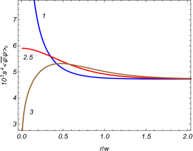
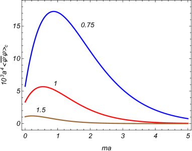
Figure 4: The part in the FC induced by compactification as a function of the radial distance from the string (left panel) and as a function of the mass (right panel). For both panels $\alpha_{0}=0.3$, $\tilde{\beta}=0.25$. The numbers near the curves are the values of the parameter $q$ for the left panel and of the ratio $L/w$ for the right panel. The graphs are plotted for $ma=1$, $L/w=1$ and for $q=2.5$, $r/w=1$ on the left and right panels, respectively.

Figure 5 presents the part $\langle\bar{\psi}\psi\rangle_{\mathrm{c}}$ in the FC as a function of $\alpha_{0}$ (left panel) and of $\tilde{\beta}$ (right panel). The left panel is plotted for $ma=0.5$, $r/w=0.5$, $L/w=1$, $\tilde{\beta}=0.25$ and the numbers near the curves correspond to the values of the parameter $q$. For the right panel we have taken $q=2$, $ma=0.5$, $r/w=0.5$, $\alpha_{0}=0.2$ and the numbers near the curves are the values of the ratio $L/w$. Considered as a function of the parameter $\tilde{\beta}$, the FC and its first derivative with respect to $\tilde{\beta}$ are continuous at half-integer values $\tilde{\beta}=\pm 1/2,\pm 3/2,\ldots$. This feature is seen from the right panel of Fig. 5. Concerning the FC as a function of the parameter $\alpha$ (containing the dependence on the magnetic flux through the cosmic string core), it is continuous at $\alpha=\pm 1/2,\pm 3/2,\ldots$, but its derivative with respect to $\alpha$ has discontinuities at those points.

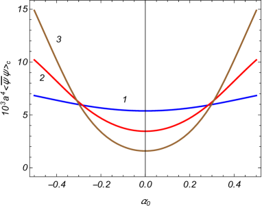
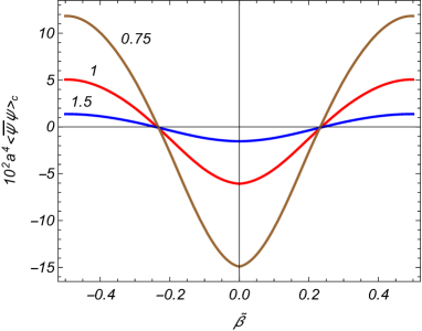
Figure 5: The condensate $\langle\bar{\psi}\psi\rangle_{\mathrm{c}}$ versus the parameters $\alpha_{0}$ and $\tilde{\beta}$. For both panels $ma=0.5$, $r/w=0.5$. The numbers near the curves are the values of the parameter $q$ for the left panel and of the ratio $L/w$ for the right panel. The graphs are plotted for $L/w=1$, $\tilde{\beta}=0.25$ and for $q=2$, $\alpha_{0}=0.2$ on the left and right panels, respectively.

Now we turn to the investigation of the FC in the asymptotic regions of the values for the compactification length. For $L/w\gg 1$ and $L/r\gg 1$, we can use again the asymptotic expression for the function ${\mathcal{Z}}_{ma}(u)$ given in (3.34). For the further estimate of the FC (4.10) two cases should be considered separately. For $2|\alpha_{0}|<1-1/q$, to the leading order, we can omit the parts $1+2\rho^{2}\sin^{2}(\pi k/q)$ and $1+2\rho^{2}\cosh^{2}u$ in (4.11) and this gives

$$\langle\bar{\psi}\psi\rangle_{\mathrm{c}}\approx-\frac{2(2ma+1)(2ma+3)}{\pi^{2}a^{4}(L/w)^{2ma+5}}\left[1+2h_{0}(q,\alpha_{0})\right]\sum_{l=1}^{\infty}\frac{\cos(2\pi l\tilde{\beta})}{l^{2ma+5}}.$$ (4.23)

This leading term does not depend on the radial coordinate $r$. In the range of the parameters $2|\alpha_{0}|>1-1/q$ we cannot ignore $2\rho^{2}\cosh^{2}u$ with respect to $(lL/w)^{2}/2$ in the integral term (the integral would diverge). This means that the dominant contribution to the integral in (4.10) comes from large values of $u$ with $e^{u}\sim L/r$. By using this fact it can be shown that for $2|\alpha_{0}|>1-1/q$ the contribution of the integral term in (4.10) dominates and to the leading order the condensate $\langle\bar{\psi}\psi\rangle_{\mathrm{c}}$ decays like $(w/r)^{2ma+5}(r/L)^{2ma+4+q-2|\alpha_{0}|q}$. In this case, the decay of the compactification contribution as a function of $1/L$ is weaker. Note that for the contribution $\langle\bar{\psi}\psi\rangle_{\mathrm{c}}^{(0)}$, by using (3.34) in (4.12), in the limit $L/w\gg 1$ one gets

$$\langle\bar{\psi}\psi\rangle_{\mathrm{c}}^{(0)}\approx-\frac{2(2ma+1)(2ma+3)}{\pi^{2}a^{4}(L/w)^{2ma+5}}\sum_{l=1}^{\infty}\frac{\cos(2\pi l\tilde{\beta})}{l^{2ma+5}}.$$ (4.24)

This leading term coincides with the part in (4.23) coming from the first term in the square brackets.

In order to find the asymptotic for small values of the ratio $L/w\ll 1$, it is convenient to provide an alternative representation for the topological part $\langle\bar{\psi}\psi\rangle_{\mathrm{t}}$. The latter is obtained by combining the representations (3.15) and (4.9) in (4.14) and by using the relation

$$\sum_{l=-\infty}^{\infty}e^{-l^{2}L^{2}x/2w^{2}+2\pi il\tilde{\beta}}=\frac{w\sqrt{2\pi}}{L\sqrt{x}}\sum_{l=-\infty}^{\infty}\exp\left[-\frac{2w^{2}\pi^{2}}{L^{2}x}\left(\tilde{\beta}-l\right)^{2}\right].$$ (4.25)

This relation directly follows from the Poisson resummation formula [69]. The required representation reads

$$\langle\bar{\psi}\psi\rangle_{\mathrm{t}} = \langle\bar{\psi}\psi\rangle_{\mathrm{c}}^{(0)}-\frac{\sqrt{2}w}{\pi^{3/2}a^{4}L}\int_{0}^{\infty}dx\,x^{3/2}e^{-x}\left[I_{\nu_{1}}(x)-I_{\nu_{2}}(x)\right]\sum_{l=-\infty}^{\infty}\exp\left[-\frac{2w^{2}\pi^{2}}{L^{2}x}\left(\tilde{\beta}-l\right)^{2}\right]$$ (4.26)

$$\times\left[\sideset{}{{}^{\prime}}{\sum}_{k=1}^{[q/2]}(-1)^{k}\cos(\pi k/q)\cos(2\pi k\alpha_{0})e^{-2x\rho^{2}\sin^{2}(\pi k/q)}\right.$$

$$\left.+\frac{q}{\pi}\int_{0}^{\infty}du\frac{h(q,\alpha_{0},2u)\sinh u}{\cosh(2qu)-\cos(q\pi)}e^{-2x\rho^{2}\cosh^{2}u}\right]\ .$$

Note that in the case of a massless field one has $I_{\nu_{1}}(x)-I_{\nu_{2}}(x)=e^{-x}\sqrt{2/\pi x}$ and the integrals over $x$ in (4.26) are expressed in terms of the function $K_{2}(4\pi|\tilde{\beta}-l|\sqrt{w^{2}+r^{2}b^{2}}/L)$ with $b=\sin(\pi k/q)$ and $b=\cosh u$ for the parts coming from the sum over $k$ and from the integral over $u$, respectively. For the first term in the right-hand side of (4.26) we will use the representation (the $k=0$ term in (4.9))

$$\langle\bar{\psi}\psi\rangle_{\mathrm{c}}^{(0)}=-\frac{1}{\pi^{2}a^{4}}\sum_{l=1}^{\infty}\cos(2\pi l\tilde{\beta})\int_{0}^{\infty}dx\,x^{2}e^{-x}\left[I_{\nu_{1}}(x)-I_{\nu_{2}}(x)\right]e^{-x(lL)^{2}/2w^{2}}.$$ (4.27)

First let us estimate this term for $L/w\ll 1$. Under this condition the dominant contribution to (4.27) comes from large values of $x$. From the corresponding asymptotic formulas for the modified Bessel function one gets $I_{\nu_{1}}\left(x\right)-I_{\nu_{2}}\left(x\right)\approx amx^{-3/2}e^{x}/\sqrt{2\pi}$ and to the leading order we obtain

$$\langle\bar{\psi}\psi\rangle_{\mathrm{c}}^{(0)}\approx-\frac{2m(w/L)^{3}}{\pi^{2}a^{3}}\sum_{l=1}^{\infty}\frac{\cos(2\pi l\tilde{\beta})}{l^{3}}.$$ (4.28)

The sum of the series in (4.28) becomes zero for $\tilde{\beta}=\tilde{\beta}_{0}\approx 0.231$. The leading term (4.28) is negative for $|\tilde{\beta}|<\tilde{\beta}_{0}$ and positive for $\tilde{\beta}_{0}<|\tilde{\beta}|\leq 0.5$. The estimate of the last term in (4.26) essentially depends on $\tilde{\beta}$. The FC is a periodic function of $\tilde{\beta}$ with the period 1 and we consider the range $|\tilde{\beta}|<1/2$. For $\tilde{\beta}=0$ the main contribution gives the term $l=0$ and the second term in the right-hand side behaves as $w/L$. In this case the first term is estimated as $\langle\bar{\psi}\psi\rangle_{\mathrm{c}}^{(0)}\approx-2m(w/L)^{3}\zeta(3)/(\pi^{2}a^{3})$ and it dominates in the total FC. For $0<|\tilde{\beta}|<1/2$, again, the contribution of the term $l=0$ dominates. Additionally assuming that $L\ll r$, we can see that the main contribution to the integral over $x$ comes from the integration range near $x\sim w/L$. Using the large argument asymptotic for the difference of the modified Bessel functions, we can see that the last term in (4.26) is suppressed by the factor $\left(Lr/w^{2}\right)^{-3/2}\exp\left[-4\pi|\tilde{\beta}|r\sin(\pi/q)/L\right]$ for $q\geq 2$ and by $\left(Lr/w^{2}\right)^{-3/2}e^{-4\pi|\tilde{\beta}|r/L}$ for $1\leq q<2$. Hence, in all cases for small values of the compactification length the FC (4.26) is dominated by the first term in the right-hand side and it behaves like $(w/L)^{3}$.

In Fig. 6 we display the dependence of the FC on the proper length of the compact dimension measured in units of the curvature radius. The graphs are plotted for $q=2.5$, $ma=0.5$, $\alpha_{0}=0.3$, $r/w=1$, and the numbers near the curves correspond to the values of the parameter $\tilde{\beta}$. The left panel presents the condensate $\langle\bar{\psi}\psi\rangle_{\mathrm{c}}^{(0)}$ for the special case of the problem with $q=1$ and $\alpha_{0}=0$ (AdS spacetime with compact dimension in the absence of the cosmic string). On the right panel we have plotted the difference $\langle\bar{\psi}\psi\rangle_{\mathrm{t}}-\langle\bar{\psi}\psi\rangle_{\mathrm{c}}^{(0)}$ (see (4.15)) that presents the effects induced by the cosmic string in AdS spacetime with a compact dimension. For $\tilde{\beta}\neq\tilde{\beta}_{0}$, the condensate $\langle\bar{\psi}\psi\rangle_{\mathrm{c}}^{(0)}$ behaves like $(w/L)^{3}$ for small values of $L/w$. For large values of that ratio the FC decays as $(w/L)^{2ma+5}$ (see (4.24)). For small values of $L/w$ and for $\tilde{\beta}=0$ we get $\langle\bar{\psi}\psi\rangle_{\mathrm{t}}-\langle\bar{\psi}\psi\rangle_{\mathrm{c}}^{(0)}\propto w/L$, whereas for $\tilde{\beta}\neq 0$ one has an exponential suppression. For large values of $L/w$ the dominant contribution in $\langle\bar{\psi}\psi\rangle_{\mathrm{t}}-\langle\bar{\psi}\psi\rangle_{\mathrm{c}}^{(0)}$ comes from the term $l=0$ in (4.15) which coincides with the condensate $\langle\bar{\psi}\psi\rangle_{\mathrm{cs}}$, given by (3.17). All these features are confirmed by the numerical results in Fig. 6.

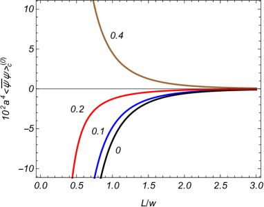
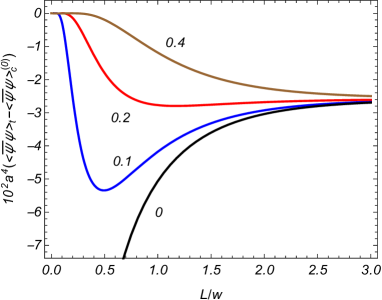
Figure 6: The contributions $\langle\bar{\psi}\psi\rangle_{\mathrm{c}}^{(0)}$ (left panel) and $\langle\bar{\psi}\psi\rangle_{\mathrm{t}}-\langle\bar{\psi}\psi\rangle_{\mathrm{c}}^{(0)}$ (right panel) in the FC as functions of the length of the compact dimension. The numbers near the curves are the values of the parameter $\tilde{\beta}$. The values of the remaining parameters are given in the text.

Now we turn to the asymptotics near the AdS boundary and horizon. For points near the AdS boundary one has $w\ll L,r$ and we use the representation (4.9). The dominant contribution to the integral over $x$ comes from the region near the lower limit. By making use of the expansion for the modified Bessel function for small values of the argument, for the leading term we get

$$\langle\bar{\psi}\psi\rangle_{\mathrm{c}} \approx -4\frac{\left(2ma+3\right)\left(2ma+1\right)}{\pi^{2}a^{4}}w^{2ma+5}\sum_{l=1}^{\infty}\cos(2\pi l\tilde{\beta})$$ (4.29)

$$\times\left[\sideset{}{{}^{\prime}_{*}}{\sum}_{k=0}^{[q/2]}\frac{(-1)^{k}\cos(\pi k/q)\cos(2\pi k\alpha_{0})}{[l^{2}L^{2}+4r^{2}\sin^{2}(\pi k/q)]^{ma+5/2}}\right.$$

$$\left.+\frac{q}{\pi}\int_{0}^{\infty}du\frac{h(q,\alpha_{0},2u)\sinh u}{\cosh(2qu)-\cos(q\pi)}\left(l^{2}L^{2}+4r^{2}\cosh^{2}u\right)^{-ma-5/2}\right]\ .$$

This shows that the compactification part in the FC vanishes on the AdS boundary as $w^{2ma+5}$. As it has been discussed in the previous section, a similar behavior takes place for the contribution $\langle\bar{\psi}\psi\rangle_{\mathrm{cs}}$ (see (3.35)).

In the near-horizon region one has $w\gg L,r$, and we consider the cases of massive and massless fields separately. Again, for a massive field we employ the representation (4.9). Now the main contribution to the integral over $x$ comes form the region with large values of $x$. For those $x$ one has

$$I_{\nu_{1}}\left(x\right)-I_{\nu_{2}}\left(x\right)\approx\frac{mae^{x}}{\sqrt{2\pi}x^{3/2}},$$

and the integrals over $x$ are expressed in terms of the gamma function. For the leading order term we get

$$\langle\bar{\psi}\psi\rangle_{\mathrm{c}} \approx -\frac{2mw^{3}}{\pi^{2}a^{3}}\sum_{l=1}^{\infty}\cos(2\pi l\tilde{\beta})\left[\sideset{}{{}^{\prime}_{*}}{\sum}_{k=0}^{[q/2]}\frac{(-1)^{k}\cos(\pi k/q)\cos(2\pi k\alpha_{0})}{\left[l^{2}L^{2}+4r^{2}\sin^{2}(\pi k/q)\right]^{3/2}}\right.$$ (4.30)

$$\left.+\frac{q}{\pi}\int_{0}^{\infty}du\frac{h(q,\alpha_{0},2u)\sinh u}{\cosh(2qu)-\cos(q\pi)}\left(l^{2}L^{2}+4r^{2}\cosh^{2}u\right)^{-3/2}\right]\ ,$$

and near the horizon the compactification induced part behaves as $w^{3}$.

For a massless field we will use the formula (4.16) for the investigation of the near-horizon asymptotic. The condensate $\langle\bar{\psi}\psi\rangle_{\mathrm{c}}$ is a periodic function of the parameter $\tilde{\beta}$ with the period 1 and in that discussion we will assume $|\tilde{\beta}|\leq 1/2$. The asymptotic is different for $\tilde{\beta}\neq 0$ and $\tilde{\beta}=0$ and we start with the first case. Under the condition (3.23) and near the horizon we can directly put $\rho=0$ in (4.16). Then, the series over $l$ is estimated by using (4.21) with $b=1$. To the leading order this gives

$$\langle\bar{\psi}\psi\rangle_{\mathrm{c}}\approx 3\frac{1+2h_{0}(q,\alpha_{0})}{32\pi^{2}a^{4}}.$$ (4.31)

By taking into account that, under same conditions, one has $\langle\bar{\psi}\psi\rangle_{\mathrm{cs}}\approx-3h_{0}(q,\alpha_{0})/(4\pi a^{2})^{2}$, for the topological part in the FC we get the asymptotic

$$\langle\bar{\psi}\psi\rangle_{\mathrm{t}}\approx\frac{3}{32\pi^{2}a^{4}}.$$ (4.32)

Recall that it is obtained under the conditions $w\gg L,r$, $\tilde{\beta}\neq 0$, $m=0$ and in the range (3.23) for the parameters. For $w\gg L,r$, $\tilde{\beta}\neq 0$, $m=0$ and in the range (3.26), the contribution from the term containing the integral over $u$ dominates in (4.16). The main contribution to the integral comes from large values of $u$ and it can be seen that, in the leading order, $\langle\bar{\psi}\psi\rangle_{\mathrm{c}}\approx-\langle\bar{\psi}\psi\rangle_{\mathrm{cs}}$, where the asymptotic for $\langle\bar{\psi}\psi\rangle_{\mathrm{cs}}$ is given by (3.27). Hence, the leading contributions coming from the separate terms in the right-hand side of the formula (4.14) for the topological FC cancel each other. Related to that, for the investigation of the behavior of the condensate $\langle\bar{\psi}\psi\rangle_{\mathrm{t}}$ in the special case under consideration it is convenient to use the representation (4.26). The dominant contribution comes from the term $\langle\bar{\psi}\psi\rangle_{\mathrm{c}}^{(0)}$ in the right-hand side and the result (4.32) is obtained for the leading term. Hence, unlike the separate contributions $\langle\bar{\psi}\psi\rangle_{\mathrm{cs}}$ and $\langle\bar{\psi}\psi\rangle_{\mathrm{c}}$, for $\tilde{\beta}\neq 0$ the condensate $\langle\bar{\psi}\psi\rangle_{\mathrm{t}}$ is finite in both regions (3.23) and (3.26).

It remains to consider the near-horizon behavior for a massless field with $\tilde{\beta}=0$. Under the condition (3.23), we substitute $\rho=0$ in (4.16) and then, by taking into account that the dominant contribution to the series comes from large $l$, replace the summation by the integration. In this way we can see that $\langle\bar{\psi}\psi\rangle_{\mathrm{c}}\approx-w/h_{0}(q,\alpha_{0})/(2\pi^{2}a^{4}L)$. Combining this with the corresponding expression for $\langle\bar{\psi}\psi\rangle_{\mathrm{cs}}$ from the previous section, one finds

$$\langle\bar{\psi}\psi\rangle_{\mathrm{t}}\approx-\frac{1+2h_{0}(q,\alpha_{0})}{4\pi^{2}a^{4}L}w.$$ (4.33)

In the range (3.26) and for $\tilde{\beta}=0$ the leading contribution in (4.16) comes from the term involving the integral over $u$. Estimating the latter in the way described above, we get

$$\langle\bar{\psi}\psi\rangle_{\mathrm{c}}\approx\frac{q\left[\left(2|\alpha_{0}|-1\right)q-1\right]w}{16\pi^{2}a^{4}L\left(\rho/2\right)^{\left(2|\alpha_{0}|-1\right)q+1}}.$$ (4.34)

In the same limit, the contribution $\langle\bar{\psi}\psi\rangle_{\mathrm{cs}}$ behaves as $1/\rho^{\left(2|\alpha_{0}|-1\right)q+1}$. Hence, for a massless field with $\tilde{\beta}=0$ near-horizon asymptotic is dominated by the contribution induced by the compactification and $\langle\bar{\psi}\psi\rangle_{\mathrm{t}}\approx\langle\bar{\psi}\psi\rangle_{\mathrm{c}}$ with $\langle\bar{\psi}\psi\rangle_{\mathrm{c}}$ given in (4.34). In this case the topological part in the FC behaves like $w^{2-\left(1-2|\alpha_{0}|\right)q}$.

Let us recall that the investigation of the effects induced by the compactification of the $z$-direction was presented in this Section in terms of the fields $\psi_{(s)}^{\prime}$ with the Lagrangian density (2.8). This means that the topological part we have discussed above corresponds to the condensate $\langle\bar{\psi}_{(s)}^{\prime}\psi_{(s)}^{\prime}\rangle_{\mathrm{c}}$. As it has been shown, it has opposite signs for the fields with $s=+1$ and $s=-1$. Returning to the initial representation with the fields $\psi_{(s)}$, having the Lagrangian density (2.4), and by taking into account the relation $\langle\bar{\psi}_{(s)}\psi_{(s)}\rangle_{\mathrm{c}}=s\langle\bar{\psi}_{(s)}^{\prime}\psi_{(s)}^{\prime}\rangle_{\mathrm{c}}$, we conclude that the compactification contributions $\langle\bar{\psi}_{(s)}\psi_{(s)}\rangle_{\mathrm{c}}$ coincide for the fields realizing two inequivalent irreducible representations of the Clifford algebra. In particular, the FC in the models invariant under the parity transformation and charge conjugation is obtained from the results given in this section with an additional coefficient 2.

In the model we have considered the only interactions of the fermionic field are with the background gravitational and electromagnetic fields. The FC is an important quantity in theories involving fermions interacting with other quantum fields. In particular, the FC appears as an order parameter that governs the phase transitions in those theories. The results obtained in the present paper can be considered as the first step in considering the combined topological effects of cosmic strings and compactification in interacting theories. The topological contributions in the FC may lead to interesting effects such as the topological mass generation, symmetry restoration and instabilities. For example, in models involving a scalar field $\varphi(x)$, with the interaction term in the Lagrangian density proportional to $\varphi^{2}\bar{\psi}\psi$, the formation of the nonzero FC leads to the term in the equation for the scalar field that is proportional to $\varphi\langle\bar{\psi}\psi\rangle$. This leads to the shift in the effective mass for $\varphi(x)$ determined by the FC (for a similar discussion for two interacting scalar fields see, e.g., [70, 71]). To the leading order with respect to the scalar-fermion interaction the mass shift is determined by the FC evaluated within the framework of the free-fermion model. Similar features may appear in Nambu-Jona-Lasinio-type four-fermion models with the self-interaction $(\bar{\psi}\psi)^{2}$ (see, for example, [2]-[11]). Again, to the leading order, the shift in the fermionic mass is determined by the condensate we have discussed above. Depending on the sign, the topological shift in the FC may lead to the restoration of the symmetries or to instabilities in interacting field theories.

5 Conclusion

In the present paper we have investigated combined effects of the gravitational field and spatial topology on the FC in (1+4)-dimensional spacetime. In order to have an exactly solvable problem, a highly symmetric background spacetime is considered with the locally AdS geometry. The nontrivial toplogy is implemented by the compactification of the $z$ coordinate and the presence of a cosmic string carrying a magnetic flux. For points outside the string’s core the influences of the cosmic string and compactification are purely topological. In odd dimensional spacetimes one has two inequivalent irreducible representations of the Clifford algebra. In order to unify the investigation of the FCs for the corresponding fields, we have passed to a new representation where the Dirac equations for those fields differ by the sign in front of the mass term.

First we have discussed the geometry where the $z$-direction has trivial topology. The contribution induced in the FC by the cosmic string is expressed as (3.17), where the function ${\mathcal{Z}}_{ma}(u)$ is given in terms of the associated Legendre function of the second kind. This contribution is an even periodic function of the magnetic flux inside the string core with the period equal to the flux quantum. The general expression for the string induced part, $\langle\bar{\psi}\psi\rangle_{\mathrm{cs}}$, is further simplified to (3.22) for a massless field. By the limiting transition we have obtained the FC around a cosmic string in (1+4)-dimensional Minkowski spacetime. For a massive field the latter is given by (3.31) and it vanishes for a massless field. This shows that the nonzero FC on the AdS bulk for massless fermionic fields is the effect induced by the gravitational field. For massive fields and at small proper distances from the string, $r_{p}\ll a$, the leading term in the asymptotic expansion for $\langle\bar{\psi}\psi\rangle_{\mathrm{cs}}$ is given by (3.33) and it diverges on the string as $1/r_{p}^{3}$. For a massless field on the AdS bulk the condensate $\langle\bar{\psi}\psi\rangle_{\mathrm{cs}}$ is finite on the string under the condition (3.23) and diverges like $1/\rho^{1+\left(2|\alpha_{0}|-1\right)q}$ in the range of parameters $2|\alpha_{0}|>1-1/q$. At large distances from the string the contribution $\langle\bar{\psi}\psi\rangle_{\mathrm{cs}}$ decays as $(w/r)^{2ma+5}$. Unlike the case of the Minkowski bulk, the fall-off in AdS bulk is power-law for both massless and massive fields.

The effects induced by the compactification of the $z$-direction are studied in Section 4. The corresponding contribution in the FC is explicitly separated by using the summation formula (4.3). For general case of a massive field it is given by the expression (4.10). For a massless field the corresponding expression is further simplified to (4.16). Because of the maximal symmetry of the AdS spacetime, the dependence of the compactification part on the variables $r$, $L$, $w$ enters in the form of the ratios $r/w$ and $L/w$. The latter is the proper length of the compact dimensions in units of the curvature radius, measured by an observer with a given value of the coordinate $w$. In the absence of the planar angle deficit and of the magnetic flux the term $k=0$, given by (4.12), survives only. The remaining part contains the effects induced by the cosmic string and magnetic flux. For both massive and massless field the compactification contribution in the FC is finite on the string for $2|\alpha_{0}|<1-1/q$ and diverges as $1/\rho^{1+\left(2|\alpha_{0}|-1\right)q}$ under the condition (3.26). This behavior is similar to that for the part $\langle\bar{\psi}\psi\rangle_{\mathrm{cs}}$ in the case of a massless field. As a limiting case, we have obtained the compactification contribution for a cosmic string in the Minkowski bulk. For a massive field it is given by the formula (4.19) and vanishes for a massless field. Hence, for a cosmic string in background of the (1+4)-dimensional Minkowski spactime with compactified $z$-direction the total FC vanishes for a massless field.

For the AdS bulk and at large proper distances from the string the FC tends to the part $\langle\bar{\psi}\psi\rangle_{\mathrm{c}}^{(0)}$ and the contribution induced by the planar angle deficit and magnetic flux decays as $(w/r)^{2ma+5}$ (see (4.22)). It is of interest to note that the leading terms in the expansions of the parts $\langle\bar{\psi}\psi\rangle_{\mathrm{cs}}$ and $\langle\bar{\psi}\psi\rangle_{\mathrm{c}}$ cancel each other and the decay of the contribution from planar angle deficit and magnetic flux in the total FC is stronger. For large values of the length of the compact dimension and under the condition (3.23) the compactification contribution decays as $(L/w)^{2ma+5}$ and the leading term in the corresponding asymptotic expansion does not depend on the radial coordinate. In the range $2|\alpha_{0}|>1-1/q$ and for large values of the compactification length the contribution $\langle\bar{\psi}\psi\rangle_{\mathrm{c}}$ behaves as $(w/r)^{2ma+5}(r/L)^{2ma+4+q-2|\alpha_{0}|q}$. In order to investigate the FC for small values of the compactification radius we have provided an alternative representation (4.26) for the topological contribution. In this limit the FC $\langle\bar{\psi}\psi\rangle_{\mathrm{t}}$ is dominated by the part $\langle\bar{\psi}\psi\rangle_{\mathrm{c}}^{(0)}$ and it behaves like $(w/L)^{3}$. The part $\langle\bar{\psi}\psi\rangle_{\mathrm{t}}-\langle\bar{\psi}\psi\rangle_{\mathrm{c}}^{(0)}$ is induced by the cosmic string and by the magnetic flux. Its behavior for small compactification radius crucially depends whether the parameter $\tilde{\beta}$, $|\tilde{\beta}|<1/2$, is zero or not. For $\tilde{\beta}=0$ one has $\langle\bar{\psi}\psi\rangle_{\mathrm{t}}-\langle\bar{\psi}\psi\rangle_{\mathrm{c}}^{(0)}\propto w/L$ and the last term in the right-hand side of (4.26) is large, though subdominant to compared with the contribution coming from $\langle\bar{\psi}\psi\rangle_{\mathrm{c}}^{(0)}$. For $0<|\tilde{\beta}|<1/2$ the effects induced by the cosmic string and by the magnetic flux corresponding to the parameter $\alpha_{0}$ are suppressed exponentially, by the factor $\exp[-4\pi|\tilde{\beta}|r\sin(\pi/q)/L]$ for $q\geq 2$ and by $e^{-4\pi|\tilde{\beta}|r/L}$ in the range $1\leq q<2$. We note that in the special case of the absence of planar angle deficit, corresponding to $q=1$, the results presented in this paper describe Aharonov-Bohm-type effects induced by magnetic fluxes in the AdS spacetime. The separate contribution to the FC for this special case are given by the formulas (3.28) and (4.18).

Both the contributions in the FC, $\langle\bar{\psi}\psi\rangle_{\mathrm{cs}}$ and $\langle\bar{\psi}\psi\rangle_{\mathrm{c}}$, tend to zero on the AdS boundary like $w^{2ma+5}$. Their behavior is more diversified near the horizon, corresponding to large values of the coordinate $w$. For a massive field the separate contributions behave as $w^{3}$. The leading terms in the corresponding asymptotic expansions are proportional to the mass. For a massless field these leading terms vanish and the near-horizon behavior of the FC is essentially different for $0<|\tilde{\beta}|\leq 1/2$ and for $\tilde{\beta}=0$. In the first case, both the parts are finite on the horizon and the limiting value for the topological condensate $\langle\bar{\psi}\psi\rangle_{\mathrm{t}}$ is expressed by (4.32). For $\tilde{\beta}=0$ and in the range of parameters (3.23), the leading term in the near-horizon expansion is given by (4.34) and the condensate behaves like $\langle\bar{\psi}\psi\rangle_{\mathrm{t}}\propto w$. Under the condition (3.26) the divergence on the horizon is stronger, as $w^{2-\left(1-2|\alpha_{0}|\right)q}$.

References

- [1] V.A. Miransky, I.A. Shovkovy, Quantum field theory in a magnetic field: From quantum chromodynamics to graphene and Dirac semimetals. Phys. Rept. 576, 1 (2015).
- [2] K.G. Klimenko, Phase structure of generalized Gross-Neveu models. Z. Phys. C 37, 457 (1988).
- [3] E. Elizalde, S. Leseduarte, S.D. Odintsov, Chiral symmetry breaking in the Nambu-Jona-Lasinio model in curved spacetime with a nontrivial topology. Phys. Rev. D 49, 5551 (1994).
- [4] T. Inagaki, T. Muta, S.D. Odintsov, Dynamical symmetry breaking in curved spacetime. Prog. Theor. Phys. Suppl. 127, 93 (1997).
- [5] P. Vitale, Temperature-induced phase transitions in four-fermion models in curved space-time. Nucl. Phys. B 551, 490 (1999).
- [6] D. Ebert, K.G. Klimenko, A.V. Tyukov, V.C. Zhukovsky, Finite size effects in the Gross-Neveu model with isospin chemical potential. Phys. Rev. D 78, 045008 (2008).
- [7] L.M. Abreu, A.P.C. Malbouisson, J.M.C. Malbouisson, A.E. Santana, Finite-size effects on the chiral phase diagram of four-fermion models in four dimensions. Nucl. Phys. B 819, 127 (2009).
- [8] D. Ebert, K.G. Klimenko, Cooper pairing and finite-size effects in a Nambu-Jona-Lasinio-type four-fermion model. Phys. Rev. D 82, 025018 (2010).
- [9] F.C. Khanna, A.P.C. Malbouisson, J.M.C. Malbouisson, A.E. Santana, Phase transition in the massive Gross-Neveu model in toroidal topologies. Phys. Rev. D 85, 085015 (2012).
- [10] A. Flachi, Interacting fermions, boundaries, and finite size effects. Phys. Rev. D 86, 104047 (2012).
- [11] A. Flachi, Dual fermion condensates in curved space. Phys. Rev. D 88, 085011 (2013).
- [12] A. Flachi, V. Vitagliano, Symmetry breaking and lattice kirigami: Finite temperature effects. Phys. Rev. D 99, 125010 (2019).
- [13] C.-S. Chu, R.-X. Miao, Fermion condensation induced by the Weyl anomaly. Phys. Rev. D 102, 046011 (2020).
- [14] C.-S. Chu, R.-X. Miao, Weyl anomaly induced Fermi condensation and holography. J. High. Energy. Phys. 08 (2020) 134.
- [15] J.B. Griffiths, J. Podolsky, Exact Space-Times in Einstein’s General Relativity (Cambridge University Press, Cambridge, England, 2009).
- [16] R. Maartens, K. Koyama, Brane-world gravity. Living Rev. Relativity 13, 5 (2010).
- [17] O. Aharony, S.S. Gubser, J. Maldacena, H. Ooguri, Y. Oz, Large N field theories, string theory and gravity. Phys. Rep. 323, 183 (2000).
- [18] M. Ammon, J. Erdmenger, Gauge/Gravity Duality: Foundations and Applications (Cambridge University Press, Cambridge, England, 2015).
- [19] A.A. Saharian, Quantum vacuum effects in braneworlds on AdS bulk. Universe 6, 181 (2020).
- [20] A. Flachi, J. Garriga, O. Pujolàs, T. Tanaka, Moduli stabilization in higher dimensional brane models. J. High Energy Phys. 08 (2003) 053.
- [21] A. Flachi, O. Pujolàs, Quantum self-consistency of AdS brane models. Phys. Rev. D 68, 025023 (2003).
- [22] E. Elizalde, M. Minamitsuji, W. Naylor, Casimir effect in rugby-ball type flux compactifications. Phys. Rev. D 75, 064032 (2007).
- [23] R. Linares, H.A. Morales-Técotl, O. Pedraza, Casimir force for a scalar field in warped brane worlds. Phys. Rev. D 77, 066012 (2008).
- [24] M. Frank, N. Saad, I. Turan, Casimir force in Randall-Sundrum models with dimensions. Phys. Rev. D 78, 055014 (2008).
- [25] A.A. Saharian, Wightman function and vacuum fluctuations in higher dimensional brane models. Phys. Rev. D 73, 044012 (2006).
- [26] A.A. Saharian, Bulk Casimir densities and vacuum interaction forces in higher dimensional brane models. Phys. Rev. D 73, 064019 (2006).
- [27] A.A. Saharian, Surface Casimir densities and induced cosmological constant in higher dimensional braneworlds. Phys. Rev. D 74, 124009 (2006).
- [28] E.R. Bezerra de Mello, A.A. Saharian, V. Vardanyan, Induced vacuum currents in anti-de Sitter space with toral dimensions. Phys. Lett. B 741, 155 (2015).
- [29] S. Bellucci, A.A. Saharian, V. Vardanyan, Vacuum currents in braneworlds on AdS bulk with compact dimensions. J. High Energy Phys. 11 (2015) 092.
- [30] S. Bellucci, A.A. Saharian, V. Vardanyan, Hadamard function and the vacuum currents in braneworlds with compact dimensions: Two-brane geometry. Phys. Rev. D 93, 084011 (2016).
- [31] S. Bellucci, A.A. Saharian, V. Vardanyan, Fermionic currents in AdS spacetime with compact dimensions. Phys. Rev. D 96, 065025 (2017).
- [32] S. Bellucci, A.A. Saharian, D.H. Simonyan, V. Vardanyan, Fermionic currents in topologically nontrivial braneworlds. Phys. Rev. D 98, 085020 (2018).
- [33] S. Bellucci, A.A. Saharian, H.G. Sargsyan, V.V. Vardanyan, Fermionic vacuum currents in topologically nontrivial braneworlds: Two-brane geometry. Phys. Rev. D 101, 045020 (2020).
- [34] T.W.B. Kibble, Some implications of a cosmological phase transition. Phys. Rep. 67, 183 (1980).
- [35] A. Vilenkin, E.P.S. Shellard, Cosmic Strings and Other Topological Defects (Cambridge University Press, Cambridge, England, 1994).
- [36] E.J. Copeland, L. Pogosian, T.Vachaspati, Seeking string theory in the cosmos. Class. Quantum Grav. 28, 204009 (2011);
- [37] D.F. Chernoff, S.-H. Henry Tye, Inflation, string theory and cosmic strings. Int. J. Mod. Phys. D 24, 1530010 (2015).
- [38] M.H. Dehghani, A.M. Ghezelbash, R.B. Mann, Vortex holography. Nucl. Phys. B 625, 389 (2002).
- [39] C.A. Ballon Bayona, C.N. Ferreira, V.J. Vasquez Otoya, A conical deficit in the AdS4/CFT3 correspondence. Class. Quantum Grav. 28, 015011 (2011).
- [40] A. de Pádua Santos, E.R. Bezerra de Mello, Non-Abelian cosmic strings in de Sitter and anti-de Sitter space. Phys. Rev. D 94, 063524 (2016).
- [41] E.R. Bezerra de Mello, A.A. Saharian, Vacuum polarization induced by a cosmic string in anti-de Sitter spacetime. J. Phys. A: Math. Theor. 45, 115402 (2012).
- [42] E.R. Bezerra de Mello, E.R. Figueiredo Medeiros, A.A. Saharian, Fermionic vacuum polarization by a cosmic string in anti-de Sitter spacetime. Class. Quantum Grav. 30, 175001 (2013).
- [43] W. Oliveira dos Santos, H.F. Mota, E.R. Bezerra de Mello, Induced current in high-dimensional AdS spacetime in the presence of a cosmic string and a compactified extra dimension. Phys. Rev. D 99, 045005 (2019).
- [44] S. Bellucci, W. Oliveira dos Santos, E.R. Bezerra de Mello, Induced fermionic current in AdS spacetime in the presence of a cosmic string and a compactified dimension. Eur. Phys. J. C 80, 963 (2020).
- [45] W. Oliveira dos Santos, E.R. Bezerra de Mello, H.F. Mota, Vacuum polarization in high-dimensional AdS space-time in the presence of a cosmic string and a compactified extra dimension. Eur. Phys. J. Plus. 135, 27 (2020).
- [46] S. Bellucci, W. Oliveira dos Santos, E.R. Bezerra de Mello, A.A. Saharian, Vacuum fermionic currents in braneworld models on AdS bulk with a cosmic string. J. High Energy Phys. 02 (2021) 190.
- [47] M. Bordag, N. Khusnutdinov, A remark on bound states in conical spacetime. Class. Quantum Grav. 13, L41 (1996).
- [48] U.H. Danielsson, E. Keski-Vakkuri, M. Kruczenski, Vacua, propagators, and holographic probes in AdS/CFT. J. High Energy Phys. 01 (1999) 002.
- [49] M. Spradlin, A. Strominger, Vacuum states for AdS2 black holes. J. High Energy Phys. 11 (1999) 021.
- [50] V.P. Frolov, E.M. Serebriany, Vacuum polarization in the gravitational field of a cosmic string. Phys. Rev. D 15, 3779 (1987).
- [51] J.S. Dowker, Vacuum averages for arbitrary spin around a cosmic string. Phys.Rev.D 36, 3742 (1987).
- [52] B. Linet, Euclidean spinor Green’s functions in the space-time of a straight cosmic string. J. Math. Phys. 36, 3694 (1995).
- [53] V.B. Bezerra, N.R. Khusnutdinov, The vacuum expectation value of the spinor massive field in the cosmic string spacetime. Class. Quantum Grav. 23, 3449 (2006).
- [54] E.R. Bezerra de Mello, V.B. Bezerra, A.A. Saharian, A.S. Tarloyan, Fermionic vacuum polarization by a cylindrical boundary in the cosmic string spacetime. Phys. Rev. D 78, 105007 (2008).
- [55] E.R. Bezerra de Mello, A.A. Saharian, S.V. Abajyan, Fermionic vacuum polarization by a flat boundary in cosmic string spacetime. Class. Quantum Grav. 30, 015002 (2013).
- [56] E.R. Bezerra de Mello, V.B. Bezerra, A.A. Saharian, V.M. Bardeghyan, Fermionic current densities induced by magnetic flux in a conical space with a circular boundary. Phys. Rev. D 82, 085033 (2010).
- [57] S. Bellucci, E.R. Bezerra de Mello, A.A. Saharian, Fermionic condensate in a conical space with a circular boundary and magnetic flux. Phys. Rev. D 83, 085017 (2011).
- [58] E.R. Bezerra de Mello, F. Moraes, A.A. Saharian, Fermionic Casimir densities in a conical space with a circular boundary and magnetic flux. Phys. Rev. D 85, 045016 (2012).
- [59] A.A. Saharian, E.R. Bezerra de Mello, A.A. Saharyan, Finite temperature fermionic condensate in a conical space with a circular boundary and magnetic flux. Phys. Rev. D 100, 105014 (2019).
- [60] S. Bellucci, I. Brevik, A.A. Saharian, H.G. Sargsyan, The Casimir effect for fermionic currents in conical rings with applications to graphene ribbons. Eur. Phys. J. C 80, 281 (2020).
- [61] A. Saharian, T. Petrosyan, A. Hovhannisyan, Casimir effect for fermion condensate in conical rings. Universe 7, 73 (2021).
- [62] I. S. Gradshteyn, I. M. Ryzhik. Table of Integrals, Series and Products (Academic Press, New York, 1980).
- [63] Handbook of Mathematical Functions, edited by M. Abramowitz, I.A. Stegun (Dover, New York, 1972).
- [64] A. A. Saharian, E. R. Bezerra de Mello, A. S. Kotanjyan, T. A. Petrosyan, Fermionic condensate in de Sitter spacetime. Astrophysics 64, 529 (2021).
- [65] E.R. Bezerra de Mello, A.A. Saharian, Topological Casimir effect in compactified cosmic string spacetime. Class. Quantum Grav. 29, 035006 (2012).
- [66] E.R. Bezerra de Mello, A.A. Saharian, Fermionic current induced by magnetic flux in compactified cosmic string spacetime. Eur. Phys. J. C 73, 2532 (2013).
- [67] S. Bellucci, E.R. Bezerra de Mello, A. de Padua, A.A. Saharian, Fermionic vacuum polarization in compactified cosmic string spacetime. Eur. Phys. J. C 74, 2688 (2014).
- [68] S. Bellucci, A. Saharian, V. Bardeghyan, Induced fermionic current in toroidally compactified spacetimes with applications to cylindrical and toroidal nanotubes. Phys. Rev. D 82, 065011 (2010).
- [69] M. A. Pinsky, Introduction to Fourier analysis and wavelets (Vol. 102). American Mathematical Soc., 2008.
- [70] L.H. Ford, Instabilities in interacting quantum field theories in non-Minkowskian spacetimes. Phys. Rev. D 22, 3003 (1980).
- [71] D.J. Toms, Symmetry breaking and mass generation by space-time topology. Phys. Rev. D 21, 2805 (1980).