Memorisation versus Generalisation in Pre-trained Language Models

Abstract

State-of-the-art pre-trained language models have been shown to memorise facts and perform well with limited amounts of training data. To gain a better understanding of how these models learn, we study their generalisation and memorisation capabilities in noisy and low-resource scenarios. We find that the training of these models is almost unaffected by label noise and that it is possible to reach near-optimal results even on extremely noisy datasets. However, our experiments also show that they mainly learn from high-frequency patterns and largely fail when tested on low-resource tasks such as few-shot learning and rare entity recognition. To mitigate such limitations, we propose an extension based on prototypical networks that improves performance in low-resource named entity recognition tasks.

1 Introduction

With recent advances in pre-trained language models Peters et al. (2018); Devlin et al. (2019); Liu et al. (2019); He et al. (2020), the field of natural language processing has seen improvements in a wide range of tasks and applications. Having acquired general-purpose knowledge from large amounts of unlabelled data, such methods have been shown to learn effectively with limited labelled data for downstream tasks Howard and Ruder (2018) and to generalise well to out-of-distribution examples Hendrycks et al. (2020).

Previous work has extensively studied what such models learn, e.g. the types of relational or linguistic knowledge Tenney et al. (2019); Jawahar et al. (2019); Rogers et al. (2020). However, the process of how these models learn from downstream data and the qualitative nature of their learning dynamics remain unclear. Better understanding of the learning processes in these widely-used models is needed in order to know in which scenarios they will fail and how to improve them towards more robust language representations.

The fine-tuning process in pre-trained language models such as BERT Devlin et al. (2019) aims to strike a balance between generalisation and memorisation. For many applications it is important for the model to generalise—to learn the common patterns in the task while discarding irrelevant noise and outliers. However, rejecting everything that occurs infrequently is not a reliable learning strategy and in many low-resource scenarios memorisation can be crucial to performing well on a task Tu et al. (2020). By constructing experiments that allow for full control over these parameters, we are able to study the learning dynamics of models in conditions of high label noise or low label frequency. To our knowledge, this is the first qualitative study of the learning behaviour of pre-trained transformer-based language models in conditions of extreme label scarcity and label noise.

We find that models such as BERT are particularly good at learning general-purpose patterns as generalisation and memorisation become separated into distinct phases during their fine-tuning. We also observe that the main learning phase is followed by a distinct performance plateau for several epochs before the model starts to memorise the noise. This makes the models more robust with regard to the number of training epochs and allows for noisy examples in the data to be identified based only on their training loss.

However, we find that these excellent generalisation properties come at the cost of poor performance in few-shot scenarios with extreme class imbalances. Our experiments show that BERT is not able to learn from individual examples and may never predict a particular label until the number of training instances passes a critical threshold. For example, on the CoNLL03 Sang and De Meulder (2003) dataset it requires 25 instances of a class to learn to predict it at all and 100 examples to predict it with some accuracy. To address this limitation, we propose a method based on prototypical networks Snell et al. (2017) that augments BERT with a layer that classifies test examples by finding their closest class centroid. The method considerably outperforms BERT in challenging training conditions with label imbalances, such as the WNUT17 Derczynski et al. (2017) rare entities dataset.

Our contributions are the following: 1) We identify a second phase of learning where BERT does not overfit to noisy datasets. 2) We present experimental evidence that BERT is particularly robust to label noise and can reach near-optimal performance even with extremely strong label noise. 3) We study forgetting in BERT and verify that it is dramatically less forgetful than some alternative methods. 4) We empirically observe that BERT completely fails to recognise minority classes when the number of examples is limited and we propose a new model, ProtoBERT, which outperforms BERT on few-shot versions of CoNLL03 and JNLPBA, as well as on the WNUT17 dataset.

2 Previous work

Several studies have been conducted on neural models’ ability to memorise and recall facts seen during their training. Petroni et al. (2019) showed that pre-trained language models are surprisingly effective at recalling facts while Carlini et al. (2019) demonstrated that LSTM language models are able to consistently memorise single out-of-distribution (OOD) examples during the very first phase of training and that it is possible to retrieve such examples at test time. Liu et al. (2020) found that regularising early phases of training is crucial to prevent the studied CNN residual models from memorising noisy examples later on. They also propose a regularisation procedure useful in this setting. Similarly, Li et al. (2020) analyse how early stopping and gradient descent affect model robustness to label noise.

Toneva et al. (2019), on the other hand, study forgetting in visual models. They find that models consistently forget a significant portion of the training data and that this fraction of forgettable examples is mainly dependent on intrinsic properties of the training data rather than the specific model. In contrast, we show that a pretrained BERT forgets examples at a dramatically lower rate compared to a BiLSTM and a non-pretrained variant.

Memorisation is closely related to generalisation: neural networks have been observed to learn simple patterns before noise Arpit et al. (2017) and generalise despite being able to completely memorise random examples Zhang et al. (2017). Zhang et al. (2021) also show that our current understanding of statistical learning theory cannot explain the super-human generalisation performance of large neural models across many areas of study.

Hendrycks et al. (2020) show that pre-trained models generalise better on out-of-distribution data and are better able to detect such data compared to non-pretrained methods but that they still do not cleanly separate in- and out-of-distribution examples. Kumar et al. (2020) find that pre-trained methods such as BERT are sensitive to spelling noise and typos. In contrast to noise in the input, we focus on the models’ learning dynamics in the presence of label noise and find that pre-trained methods are remarkably resilient to such cases.

3 Experimental setting

We investigate the performance of pre-trained language models in specific adverse conditions. In order to evaluate generalisation abilities, we first create datasets with varying levels of label noise by randomly permuting some of the labels in the training data. This procedure allows us to pinpoint noisy examples and evaluate the performance on clean and noisy datapoints separately. Then, in order to investigate memorisation we train the models on datasets that contain only a small number of examples for a particular class. This allows us to evaluate how well the models are able to learn from individual datapoints as opposed to high-frequency patterns. We make the code for the experiments available online.

Datasets

We focus on the task of named entity recognition (NER) and employ the CoNLL03 Sang and De Meulder (2003), the JNLPBA Collier and Kim (2004), and the WNUT17 Derczynski et al. (2017) datasets. NER is commonly used for evaluating pre-trained language models on structured prediction and its natural class imbalance is well suited for our probing experiments. CoNLL03 and JNLPBA are standard datasets for NER and Bio-NER respectively. The WNUT17 dataset is motivated by the observation that state-of-the-art methods tend to memorise entities during training Augenstein et al. (2017). The dataset focuses on identifying unusual or rare entities at test time that cannot be simply memorised by the model. We evaluate based on entity-level F₁ unless stated otherwise.

Language models

We use BERT-base Devlin et al. (2019) as the main language model for our experiments, as BERT is widely used in practice and other variations of pre-trained language models build on a similar architecture. The model is augmented with a classification feed-forward layer and fine-tuned using the cross-entropy loss with a learning rate of $10^{-4}$. AdamW Loshchilov and Hutter (2019) is used during training with weight decay of 0.01 and a linear warm-up rate of 10%. The test results are recorded using the model that produced the highest validation metrics.

We compare BERT’s behaviour with that of other pre-trained transformers such as RoBERTa Liu et al. (2019) and DeBERTa He et al. (2020) fine-tuned with the same optimiser and hyper-parameters as above. In order to also compare against non-transformer models, we report performance for a bi-LSTM-CRF Lample et al. (2016) model with combined character-level and word-level representations. The model is comprised of 10 layers, with 300-dimensional word representations and 50-dimensional character representations, for a total of approximately 30 million trainable parameters. In our experiments, the model is trained with the Adam optimiser Kingma and Ba (2014) and a learning rate of $10^{-4}$ for 100 epochs using a CRF loss Lafferty et al. (2001).

4 Generalisation in noisy settings

We first investigate how BERT learns general patterns from datasets that contain label noise. Figure 1 shows how the model performance on the CoNLL03 training and validation sets changes when faced with varying levels of noise, from 0% to 50%. Based on the progression of performance scores, we can divide BERT’s learning process into roughly three distinct phases:

1. Fitting: The model uses the training data to learn how to generalise, effectively learning simple patterns that can explain as much of the training data as possible Arpit et al. (2017). Both the training and validation performance rapidly increase as the model learns these patterns.

2. Settling: The increase in performance plateaus and neither the validation nor the training performance change considerably. The duration of this phase seems to be inversely proportional to the amount of noise present in the dataset.

3. Memorisation: The model rapidly starts to memorise the noisy examples, quickly improving the performance on training data while degrading the validation performance, effectively over-fitting to the noise in the dataset.

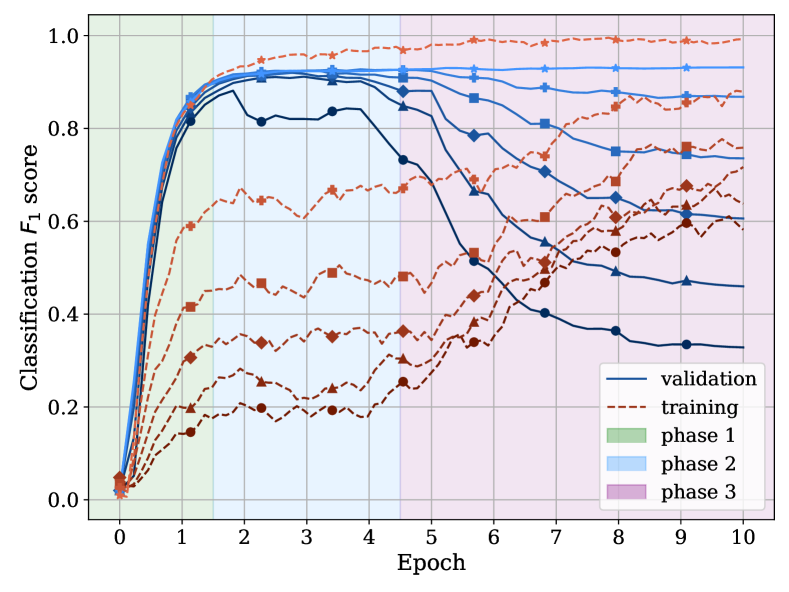
Figure 1: BERT performance (F₁) throughout the training process on the CoNLL03 train and validation sets. Darker colours correspond to higher levels of noise (0% to 50%).

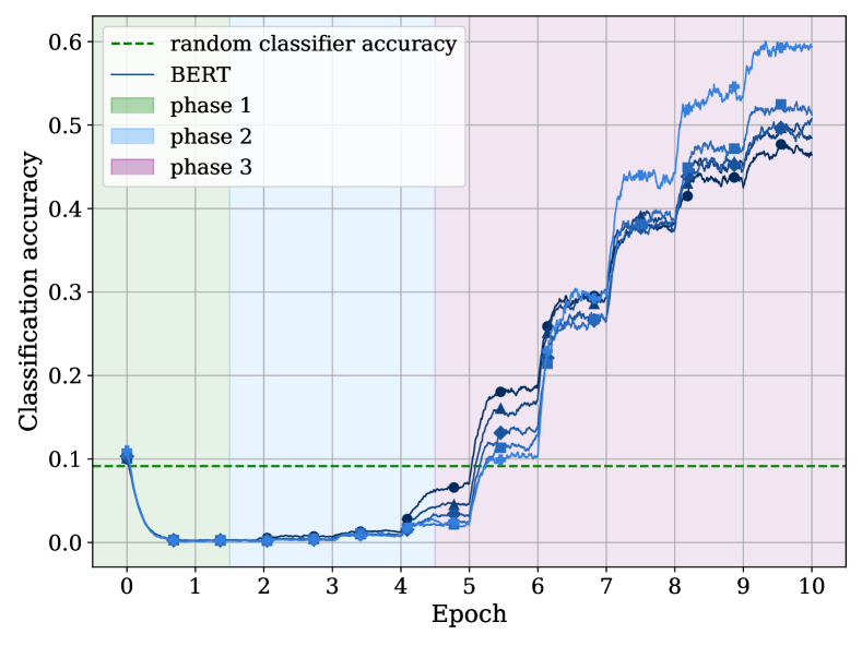
Figure 2: Classification accuracy of noisy examples in the training set for the CoNLL03 dataset. Darker colours correspond to higher levels of noise (0% to 50%).

A second phase of learning

We find BERT to exhibit a distinct second settling phase during which it does not over-fit. A resilience to label noise has been observed in other neural networks trained with gradient descent Li et al. (2020). However, we find this phase to be much more prolonged in BERT compared to models pre-trained on other modalities such as a pre-trained ResNet fine-tuned on CIFAR10, which immediately starts memorising noisy examples (see Appendix A for a comparison). These results indicate that the precise point of early stopping is not as important when it comes to fine-tuning pre-trained language models. Similar optimal performance is retained for a substantial period, therefore training for a fixed number of epochs can be sufficient.

We illustrate BERT’s behaviour by evaluating the token-level classification accuracy of noisy examples in Figure 2. During the second phase, BERT completely ignores the noisy tokens and correctly misclassifies them, performing “worse” than a random classifier. The step-like improvements during the third stage show that the model is unable to learn any patterns from the noise and improves by repeatedly optimising on the same examples, gradually memorising them.

Robustness to noise

We also observe in Figure 1 that BERT is extremely robust to noise and over-fitting in general. In the absence of noise, the model does not over-fit and maintains its development set performance, regardless of the length of training. Even with a large proportion of noise, model performance comparable to training on the clean dataset can be achieved by stopping the training process somewhere in the second phase.

We also hypothesise that due to the robustness to noise shown in the second phase of training, a noise detector can be constructed based only on BERT’s training losses, without requiring any other information. We find that a simple detector that clusters the losses using k-means reliably achieves over 90% noise-detection F₁ score in all our experiments, further showing how the model is able to actively detect and reject single noisy examples (see Appendix E for details about the noise detection process).

Impact of pre-training

The above properties can mostly be attributed to BERT’s pre-training process—after large-scale optimisation as a language model, the network is primed for learning general patterns and better able to ignore individual noisy examples. We find that a randomly initialised model with the same architecture does not only achieve lower overall performance but crucially does not exhibit’s BERT’s distinct second phase of learning and robustness to noise (see Appendix C).

Other pre-trained transformers

We also analyse the behaviour of other pre-trained transformers for comparison. Specifically, studying RoBERTa and DeBERTa, we find the same training pattern that was observed in BERT—all models show a clear division into the three phases described above. These models are also all very robust to label noise during the settling phase of training. Notably, RoBERTa is even more resilient to label noise compared to the other two analysed models, despite DeBERTa outperforming it on public benchmarks He et al. (2020). Training and validation performance visualisations, such as those in Figure 1, can be found for both models in Appendix I.

5 Forgetting of learned information

Evaluating only the final model does not always provide the full picture regarding datapoint memorisation, as individual datapoints can be learned and forgotten multiple times during the training process. Following Toneva et al. (2019), we record a forgetting event for an example at epoch $t$ if the model was able to classify it correctly at epoch $t-1$, but not at epoch $t$. Similarly, we identify a learning event for an example at epoch $t$ if the model was not able to classify it correctly at epoch $t-1$, but it is able to do so at epoch $t$. A first learning event thus happens at the first epoch when a model is able to classify an example correctly. We furthermore refer to examples with zero and more than zero forgetting events as unforgettable and forgettable examples, respectively, while the set of learned examples includes all examples with one or more learning events.

In Table 1, we show the number of forgettable, unforgettable, and learned examples on the training data of the CoNLL03 and JNLPBA datasets for BERT, a non-pre-trained BERT, and a bi-LSTM model. We also show the ratio between forgettable and learned examples, which indicates how easily a model forgets learned information. We can observe that BERT forgets less than other models and that pre-training is crucial for retaining important information. We show the most forgettable examples in Appendix D, which tend to be atypical examples of the corresponding class.

Dataset	Model	Forgettable $N_{f}$	Unforgettable $N_{u}$	Learned $N_{l}$	$N_{f}/N_{l}$ (%)
CoNNL03	bi-LSTM	71.06%	29.94%	90.90%	78.17%
	non-pre-trained BERT	9.89%	90.11%	99.87%	9.90%
	pre-trained BERT	2.97%	97.03%	99.80%	2.98%
JNLPBA	bi-LSTM	97.16%	5.14%	98.33%	98.81%
	non-pre-trained BERT	25.50%	74.50%	98.24%	25.96%
	pre-trained BERT	16.62%	83.38%	98.18%	16.93%

Table 1: Number of forgettable, unforgettable, and learned examples during BERT training on the CoNLL03 dataset and JNLPBA dataset.

Toneva et al. (2019) found that the number of forgetting events remains comparable across different architectures for the vision modality, given a particular dataset. However, our experiments show that the same does not necessarily hold for pre-trained language models. Specifically, there is a large discrepancy in the ratio between forgettable and learned examples for BERT ($\scriptstyle\sim$3%) and a bi-LSTM model ($\scriptstyle\sim$80%) on the CoNLL03 dataset.

We additionally analyse the distribution of first learning events throughout BERT’s training on CoNLL03 with label noise between 0% and 50% (Figure 3) and notice how BERT learns the majority of learned examples during the first epochs of training. As the training progresses, we see that BERT stops learning new examples entirely, regardless of the level of noise for the third and fourth epochs. Finally, in the last epochs BERT mostly memorises the noise in the data.

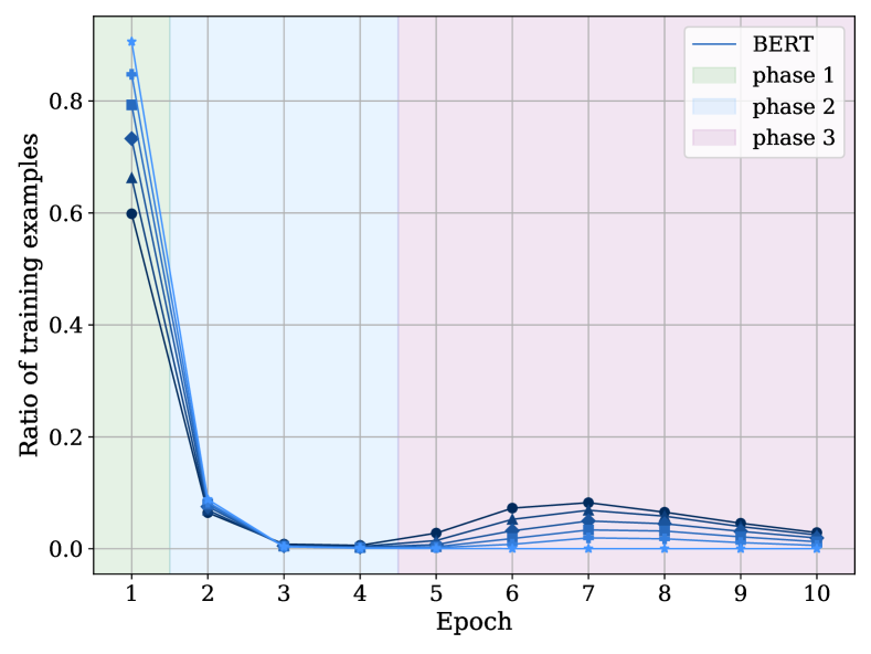
Figure 3: First learning events distribution during the training for various levels of noise on the CoNLL03 dataset. Darker colours correspond to higher levels of noise (0% to 50%).

6 BERT in low-resource scenarios

In the previous sections, we have observed that BERT learns examples and generalises very early in training. We will now examine if the same behaviour applies in low-resource scenarios where a minority class is only observed very few times. To this end, we remove from the CoNLL03 training set all sentences containing tokens with the minority labels MISC and LOC except for a predetermined number of such sentences. We repeat the process for the JNLPBA dataset with the DNA and Protein labels.

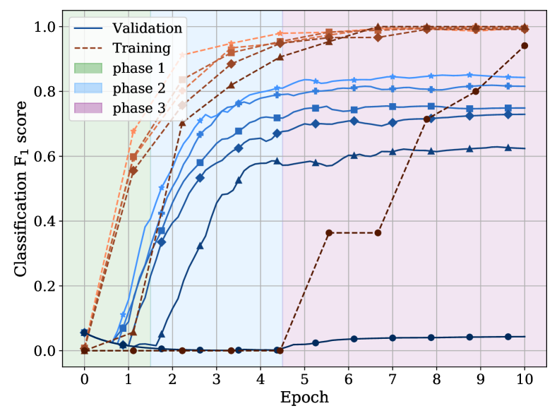
Figure 4: BERT performance (F₁) throughout the training process on the CoNLL03 dataset with varying number of sentences containing the LOC class. Darker colours correspond to fewer examples of the LOC class available (5 to 95 in steps of 20).

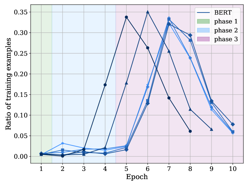
Figure 5: First learning events distribution during the training on the CoNLL03 dataset with varying number of sentences containing the LOC class. Darker colours correspond to fewer examples of the LOC class available (5 to 95 in steps of 20).

We conduct similar experiments to the previous sections by studying how different numbers of sentences containing the target class affect BERT’s ability to learn and generalise. We report in Figure 4 the training and validation classification F₁ score for the CoNLL03 datasets from which all but few (5 to 95) sentences containing the LOC label were removed. Note that the reported performance in this experiment refers to the LOC class only. In Figure 5 we also report the distribution of first learning events for the LOC class in the same setting. Two phenomena can be observed: 1) reducing the number of sentences greatly reduces the model’s ability to generalise (validation performance decreases yet training performance remains comparable); and 2) when fewer sentences are available, they tend to be learned in earlier epochs for the first time. Corresponding experiments on the MISC label can be found in Appendix J.

We also show the average entity-level F₁ score on tokens belonging to the minority label and the model performance for the full NER task (i.e. considering all classes) for the CoNLL03 and JNLPBA datasets in Figures 6 and 7 respectively. For the CoNLL03 dataset, we observe that BERT needs at least 25 examples of a minority label in order to be able to start learning it. Performance rapidly improves from there and plateaus at around 100 examples. For the JNLPBA dataset, the minimum number of examples increases to almost 50 and the plateau occurs for a higher number of examples. On the challenging WNUT17 dataset, BERT achieves only 44% entity-level F₁. This low performance is attributable to the absence of entity overlap between training set and test set, which increases the inter-class variability of the examples.

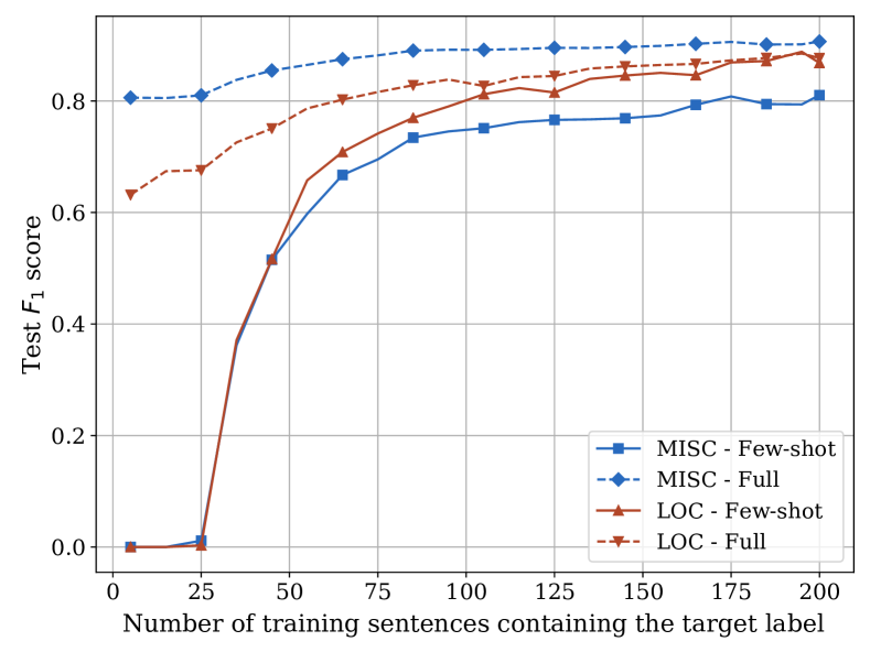
Figure 6: BERT final validation entity-level F₁ score on the few-shot class keeping varying numbers of sentences containing examples of a selected class on the CoNLL03 dataset.

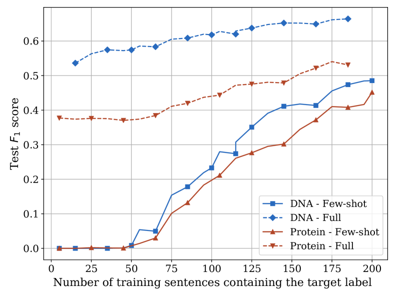
Figure 7: BERT final validation entity-level F₁ score on the few-shot class keeping varying numbers of sentences containing examples of a selected class on the JNLPBA dataset.

7 ProtoBERT for few-shot learning

In order to address BERT’s limitations in few-shot learning, we propose a new model, ProtoBERT that combines BERT’s pre-trained knowledge with the few-shot capabilities of prototypical networks Snell et al. (2017) for sequence labelling problems. The method builds an embedding space where the inputs are clustered on a per-class basis, allowing us to classify a token by finding its closest centroid and assigning it the corresponding class. The model can be seen in Figure 8.

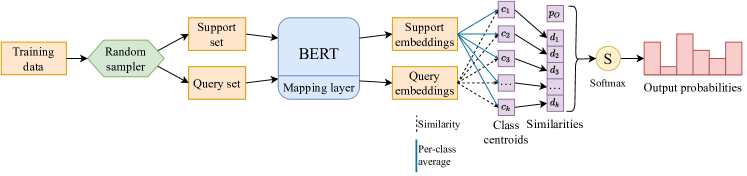
Figure 8: Schematic representation of the inference using a BERT model with a prototypical network layer.

We first define a support set $S$, which we use as context for the classification and designate with $S_{k}$ all elements of $S$ that have label $k$. We refer to the set of points that we want to classify as the query set $Q$, with $l(Q_{i})$ indicating the label of the $i^{\text{th}}$ element in $Q$. We will also refer to $f$ as the function computed by BERT augmented with a linear layer, which produces an $M$ dimensional output.

The model then classifies a given input $\mathbf{x}$ as follows: for each class $k$, we compute the centroid of the class in the learned feature space as the mean of all the elements that belong to class $k$ in the support set $S$:

$$\mathbf{c}_{k}=\frac{1}{|S_{k}|}\sum_{\mathbf{x}_{i}\in S_{k}}f(\mathbf{x}_{i})$$ (1)

Then, we compute the distance from each input $\mathbf{x}\in Q$ to each centroid:

$$dist_{k}=d(f(\mathbf{x}),\mathbf{c}_{k})$$

and collect them in a vector $v\in\mathbb{R}^{k}$. Finally, we compute the probability of $\mathbf{x}$ belonging to class $k$ as

$$p(y=k\mid\mathbf{x}) =\frac{\exp\left(-d\left(f(\mathbf{x}),\mathbf{c}_{k}\right)\right)}{\sum_{k^{\prime}}\exp\left(-d\left(f(\mathbf{x}),\mathbf{c}_{k^{\prime}}\right)\right)}=$$

$$=softmax(-v)_{k}$$

The model is trained by optimising the cross-entropy loss between the above probability and the one-hot ground-truth label of $\mathbf{x}$. Crucially, $S$ and $Q$ are not a fixed partition of the training set but change at each training step. Following Snell et al. (2017), we use Euclidean distance as a choice for the function $d$.

In order to take into account the extreme under-representation of some classes, we create the support by sampling $s_{1}$ elements from each minority class and $s_{2}$ elements from each non-minority class. A high ratio $s_{1}/s_{2}$ gives priority to the minority classes, while a low ratio puts more emphasis on the other classes. We then similarly construct the query set with a fixed ratio $n$ between the minority classes and the non-minority classes.

For NER, rather than learning a common representation for the negative class “O”, we only want the model to treat it as a fallback when no other similar class can be found. For this reason, we define the vector of distances $v$ as follows:

$$v=(d_{O},\ dist_{0},\ \ldots,\ dist_{k})$$

where $d_{O}$ is a scalar parameter of the network that is trained along with the other parameters. Intuitively, we want to classify a point as a non-entity (i.e. class O) when it is not close enough to any centroid, where $d_{O}$ represents the threshold for which we consider a point “close enough”.

If no example of a certain class is available in the support set during the training, we assign a distance of $400$, making it effectively impossible to mistakenly classify the input as the missing class during that particular batch. Finally, we propose two ways to compute the class of a token at test time. The first method employs all examples from $X$ to calculate the centroids needed at test time, which produces better results but is computationally expensive for larger datasets.

The second method approximates the centroid $\mathbf{c}_{k}$ using the moving average of the centroids produced at each training step:

$$\mathbf{c}_{k}^{(t)}\leftarrow\alpha\ \mathbf{c}_{k}^{(t)}\cdot(1-\alpha)\ \mathbf{c}_{k}^{(t-1)}$$

where $\alpha$ is a weighting factor. This method results in little overhead during training and only performs marginally worse than the first method.

7.1 Experimental results

We first compare ProtoBERT to the standard pre-trained BERT model with a classification layer on the CoNLL03 and JNLPBA datasets with a smaller number of sentences belonging to the minority classes. We show the results on the few-shot classes and for the full dataset for CoNLL03 in Figures 9 and 10 respectively. Similarly, we show the results for the few-shot class for JNLPBA in Figure 11. In all cases ProtoBERT consistently surpasses the performance of the baseline when training on few examples of the minority class. It particularly excels in the extreme few-shot setting, e.g. outperforming BERT by 40 F₁ points with 15 sentences containing the LOC class. As the number of available examples of the minority class increases, BERT starts to match ProtoBERT’s performance and outperforms it on the full dataset in some cases.

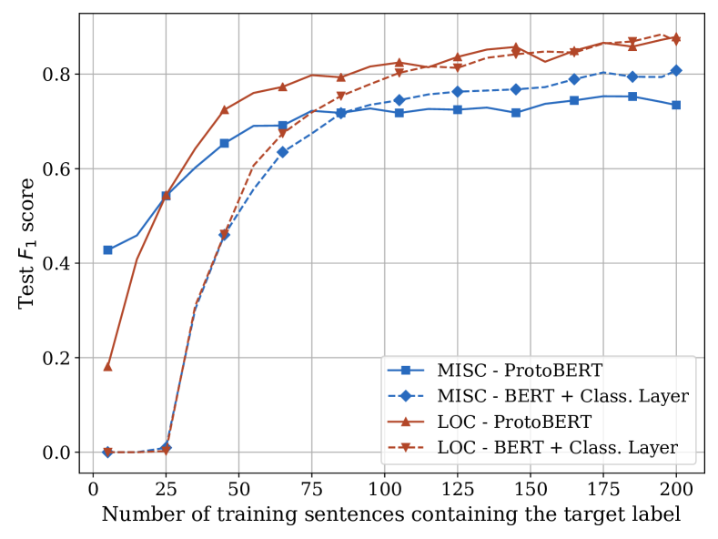
Figure 9: Model performance comparison between the baseline model and ProtoBERT for the CoNLL03 dataset, reducing the sentences containing the MISC and LOC classes. Results reported as F₁ score on the few-shot classes.

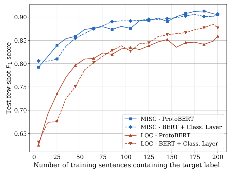
Figure 10: Model performance comparison between the baseline model and ProtoBERT for the CoNLL03 dataset, reducing the sentences containing the MISC and LOC class. Results reported as F₁ score on all classes.

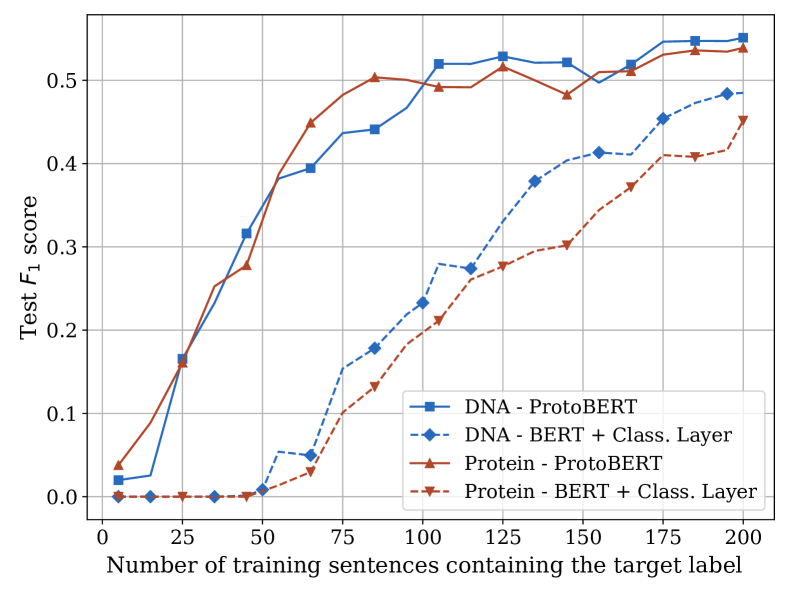
Figure 11: Model performance comparison between the baseline model and ProtoBERT for the JNLPBA dataset, reducing the sentences containing the DNA and Protein classes. Results reported as F₁ score on the few-shot classes.

Model	CoNLL03	JNLPBA	WNUT17
State of the art	93.50	77.59	50.03
BERT + classification layer (baseline)	89.35	75.36	44.09
ProtoBERT	89.87	73.91	48.62
ProtoBERT + running centroids	89.46	73.54	48.56

Table 2: Comparison between the baseline model, the current state-of-the-artand the proposed architecture on the CoNLL03, JNLPBA and WNUT17 datasets evaluated using entity-level F₁ score. The state of the art is Baevski et al. (2019), Lee et al. (2019), and Wang et al. (2019) respectively.

While the main strength of ProtoBERT is on few-shot learning, we evaluate it also on the full CoNLL03, JNLPBA and WNUT17 datasets (without removing any sentences) in Table 7. In this setting, the proposed architecture achieves results mostly similar to the baseline while considerably outperforming it on the WNUT17 dataset of rare entities.

The results in this section show that ProtoBERT, while designed for few-shot learning, performs at least on par with its base model in all tasks. This allows the proposed model to be applied to a much wider range of tasks and datasets without negatively affecting the performance if no label imbalance is present, while bringing a substantial improvement in few-shot scenarios.

We conduct an ablation study to verify the effect of our improved centroid computation method. From the results in Table 7 we can affirm that, while a difference in performance does exist, it is quite modest (0.1–0.4%). On the other hand, this method reduces the training time and therefore energy consumption Strubell et al. (2019) to one third of the original method on CoNLL03 and we expect the reduction to be even greater for larger datasets.

8 Conclusion

In this study, we investigated the learning process during fine-tuning of pre-trained language models, focusing on generalisation and memorisation. By formulating experiments that allow for full control over the label distribution in the training data, we study the learning dynamics of the models in conditions of high label noise and low label frequency. The experiments show that BERT is capable of reaching near-optimal performance even when a large proportion of the training set labels has been corrupted. We find that this ability is due to the model’s tendency to separate the training into three distinct phases: fitting, settling, and memorisation, which allows the model to ignore noisy examples in the earlier epochs. The pretrained models experience a prolonged settling phase when fine-tuned, during which their performance remains optimal, indicating that the precise area of early stopping is less crucial.

Furthermore, we show that the number of available examples greatly affects the learning process, influencing both when the examples are memorised and the quality of the generalisation. We show that BERT fails to learn from examples in extreme few-shot settings, completely ignoring the minority class at test time. To overcome this limitation, we augment BERT with a prototypical network. This approach partially solves the model’s limitations by enabling it to perform well in extremely low-resource scenarios and also achieves comparable performance in higher-resource settings.

Appendix A Comparison of learning phases in a BiLSTM and ResNet on CIFAR-10

For comparison, we show the training progress of a ResNet He et al. (2015) trained on CIFAR10 Krizhevsky (2009) in Figure 12. Following Toneva et al. (2019), we use a ResNeXt model Xie et al. (2017) with 101 blocks pre-trained on the ImageNet dataset Deng et al. (2009). The model has been fine-tuned with a cross-entropy loss with the same optimiser and hyper-parameters as BERT. We evaluate it using F₁ score. As can be seen, the training performance continues to increase while the validation performs plateaus or decreases, with no clearly delineated second phase as in the pre-trained BERT’s training.

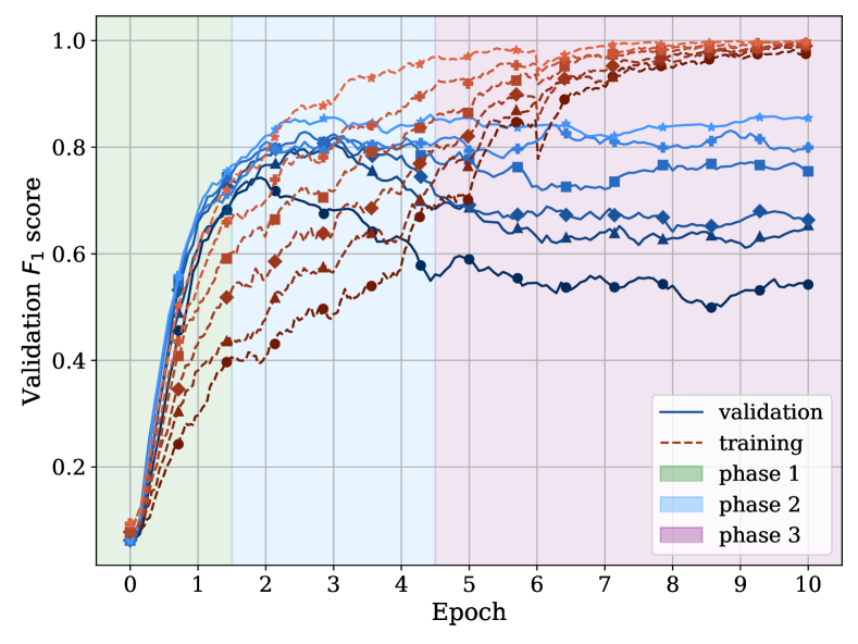
Figure 12: Performance (F₁) of a ResNet model throughout the training process on the CIFAR10 dataset. Darker colours correspond to higher levels of noise (0% to 50%).

Appendix B JNLPBA noise results

As well as CoNLL03, we also report the analysis on the JNLPBA dataset. In Figure 13, we show the performance of BERT on increasingly noisy versions of the training set. In Figure 14, we report the accuracy of noisy examples.

Figure 13: BERT performance (F₁) throughout the training process on the JNLPBA dataset. Darker colours correspond to higher levels of noise (0% to 50%).

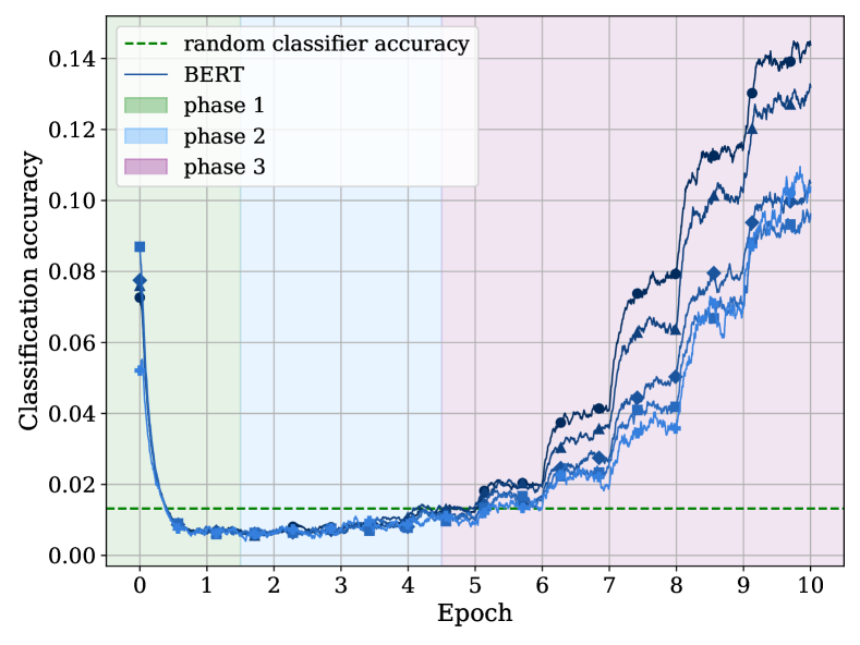
Figure 14: Classification accuracy of noisy examples in the training set for the JNLPBA dataset. Darker colours correspond to higher levels of noise (0% to 50%).

Appendix C Effect of pre-training

BERT’s second phase of pre-training and noise resilience are mainly attributable to its pre-training. We show the training progress of a non-pretrained BERT model on CoNLL03 in Figure 15 and its classification accuracy on noisy examples in Figure 16. As can be seen, a non-pre-trained BERT’s training performance continuously improves and so does its performance on noisy examples.

Figure 15: Performance (F₁) of a non-pre-trained BERT model throughout the training process on the CoNLL03 train and validation sets. Darker colours correspond to higher levels of noise (0% to 50%).

Figure 16: Classification accuracy of a non-pre-trained BERT model on noisy examples in the training set for the CoNLL03 dataset. Darker colours correspond to higher levels of noise (0% to 50%).

Appendix D Examples of forgettable examples

In Table 3, we can find the sentences containing the most forgettable examples during a training run of 50 epochs for the CoNLL03 dataset. The maximum theoretical number of forgetting events in this case is 25. It is important to notice how the most forgotten entity presents a mismatched "The", which the network correctly classifies as an "other" (O) entity.

Sentence	Number of forgetting events
the third and final test between England and Pakistan at The (I-LOC)	11
GOLF - BRITISH MASTERS THIRD ROUND SCORES . (O)	10
GOLF - GERMAN OPEN FIRST ROUND SCORES . (O)	10
English County Championship cricket matches on Saturday : (MISC)	10
English County Championship cricket matches on Friday : (MISC)	9

Table 3: Sentences containing the most forgettable examples in the CoNLL03 dataset. In bold the entity that was most often forgotten within the given sentence and in brackets its ground-truth classification.

Appendix E BERT as a noise detector

We report the exact detection metrics for the model proposed in section 4 in Table 4. Here we can see how both for extremely noisy datasets and for cleaner datasets, our model is able to detect the noisy examples with about 90-91% F₁ score, as mentioned above.

Noise	Precision	Recall	F1 score
10%	92.18%	95.90%	94.00%
20%	96.19%	96.33%	96.26%
30%	98.02%	96.35%	97.17%
40%	98.27%	96.95%	97.60%
50%	98.64%	97.27%	97.94%

Table 4: Noise detection performance with varying levels of noise on the CoNLL03 dataset using the method proposed.

Moreover, we provide the implementation used to detect outliers used to produce the table and figures above:

1. We first collect the losses for each training example after a short fine-tuning process (4 epochs in our case).

2. We then assume an unknown portion of these examples is noisy, giving rise to a two-class classification problem (noisy vs non-noisy). To discriminate the two classes, we then solve the following optimisation problem which aims to find a loss threshold $T$ that minimises inter-class variance for each of the two classes:

   $$\underset{T}{\arg\min}\sum_{x\ <\ T}\left\|x-\mu_{c}\right\|^{2}+\sum_{x\ \geq\ T}\left\|x-\mu_{n}\right\|^{2}$$

   Where elements denoted as $x$ are the losses extracted from the training set, $\mu_{c}$ is the mean of all $x<T$, and $\mu_{n}$ is the mean of all $x\geq T$.

3. For testing purposes, we then apply the method to the chosen training set and measure the noise detection F1 score.

In Figure 17, we qualitatively saw how the losses are distributed for noisy and regular examples and notice how they are neatly separated except for a small subset of the noisy examples. These examples might have been already memorised by the model, which would explain their lower loss.

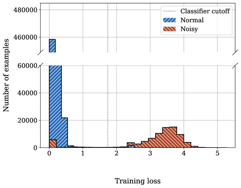
Figure 17: Loss distribution for noisy and non-noisy examples from the CoNLL03 training set. The grey dashed line represent the chosen loss threshold found by our method to discriminate between noisy and non-noisy examples.

Appendix F JNLPBA forgetting results

We show in Figure 18 how many data points were learned by BERT for the first time at each epoch on the JNLPBA dataset during training (first learning events).

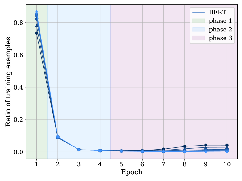
Figure 18: First learning events distribution during BERT training for various levels of noise on the JNLPBA dataset. Darker colours correspond to higher levels of noise (0% to 50%).

Appendix G Further ProtoBERT results

As in Table 7 we only reported F₁ score for our methods, for completeness we also report precision and recall in table 5.

Model	CoNLL03			JNLPBA			WNUT17
	P	R	F1	P	R	F1	P	R	F1
State-of-the-art	NA	NA	93.50	NA	NA	77.59	NA	NA	50.03
BERT + classification layer (baseline)	88.97	89.75	89.35	72.99	77.90	75.36	53.65	37.42	44.09
ProtoBERT	89.26	90.49	89.87	68.66	80.03	73.91	54.38	43.96	48.62
ProtoBERT + running centroids	89.03	89.91	89.46	68.92	78.83	73.54	54.11	44.05	48.56

Table 5: Comparison between the baseline model and the proposed architecture on the CoNLL03, JNLPBA and WNUT17 datasets evaluated using entity-level metrics.

Noise	Forgettable	Unforgettable	Learned	Forgettable/learned (%)
CoNLL03 0%	2,669	699,381	230,716	1.1568%
CoNLL03 10%	10,352	691,698	224,968	4.6015%
CoNLL03 20%	19,667	682,383	216,780	9.0723%
CoNLL03 30%	30,041	672,009	209,191	14.3606%
JNLPBA 0%	23,263	817,087	457,485	5.0849%
JNLPBA 10%	26,667	813,683	422,264	6.3152%
JNLPBA 20%	26,369	813,981	386,562	6.8214%
JNLPBA 30%	30,183	810,167	353,058	8.5490%
CIFAR10 0%	8,328	36,672	45,000	18.5067%
CIFAR10 10%	9,566	35,434	44,976	21.2691%
CIFAR10 20%	9,663	35,337	44,922	21.5106%
CIFAR10 30%	11,207	33,793	44,922	24.9477%

Table 6: Number of forgettable, unforgettable, and learned examples during BERT training on the CoNLL03, JNLPBA and CIFAR10 datasets.

Examples	BERT	bi-LSTM
Forgettable	2,669	144,377
Unforgettable	699,381	60,190
Learned	230,716	184,716
Forgettable/learned (%)	1.1568%	78,1616%

Table 7: Comparison of the number of forgettable, learnable and unforgettable examples between BERT and a bi-LSTM model.

Appendix H ProtoBERT results on JNLPBA

We report in Figure 19 the comparison between our baseline and ProtoBERT for all classes.

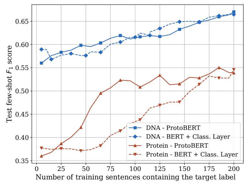
Figure 19: Model performance comparison between the baseline model and ProtoBERT for the JNLPBA dataset, reducing the sentences containing the DNA and Protein class. Results reported as F₁ score on all classes.

Appendix I Results on other pretrained transformers

While most of the main paper focuses on BERT, it is worthwhile to mention the results on other pre-trained transformers and compare the results.

In Figures 20 and 21, we show the validation performances (classification F₁ score) for the CoNLL03 datasets for the RoBERTa and DeBERTa models (similarly to Figure 1). We notice that the three phases of training reported above are apparent in all studied models. RoBERTa, in particular, displays the same pattern, but shows higher robustness to noise compared to the other two models.

Moreover, in Figures 22 and 23, we report the distribution of first learning events (similarly to Figure 5) on RoBERTa and DeBERTa. As above, we can observe the same pattern described in the main body of the paper, with the notable exception that RoBERTa is again more robust to learning the noise in later phases of the training.

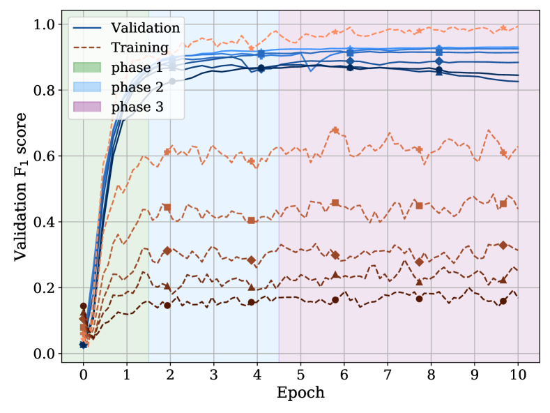
Figure 20: RoBERTa performance (F₁) throughout the training process on the CoNLL03 train and validation sets. Darker colours correspond to higher levels of noise (0% to 50%).

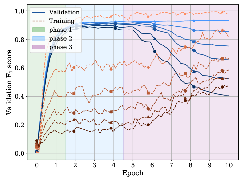
Figure 21: DeBERTa performance (F₁) throughout the training process on the CoNLL03 train and validation sets. Darker colours correspond to higher levels of noise (0% to 50%).

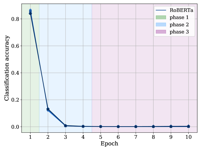
Figure 22: First learning events distribution during RoBERTa training for various levels of noise on the CoNLL03 dataset. Darker colours correspond to higher levels of noise (0% to 50%).

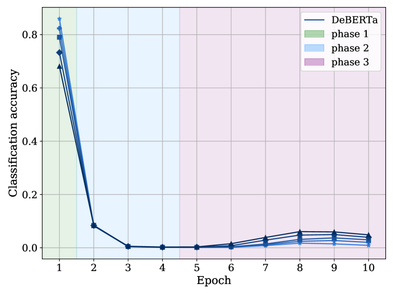
Figure 23: First learning events distribution during DeBERTa training for various levels of noise on the CoNLL03 dataset. Darker colours correspond to higher levels of noise (0% to 50%).

Appendix J Few-shot MISC memorisation

As per section 6, we also report the result of the experiments in the few-shot setting by removing most sentences containing the MISC class. The experimental setting is identical to the described in the main body of the paper. The relevant Figures are 24 and 25.

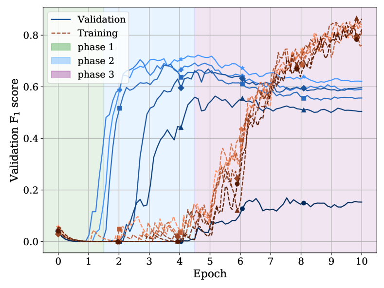
Figure 24: BERT performance (F₁) throughout the training process on the CoNLL03-XMISC train and validation sets. Darker colours correspond to fewer examples of the MISC class available (5 to 95 in steps of 20).

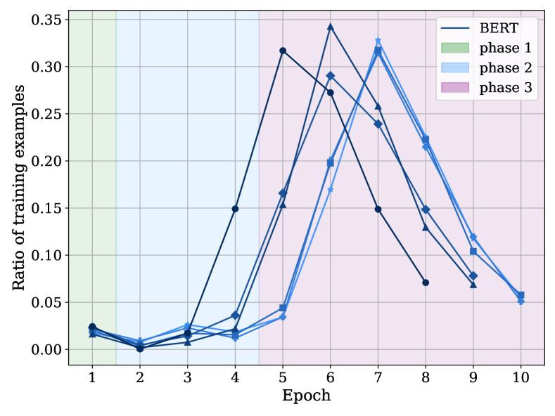
Figure 25: First learning events distribution during the training for various levels of noise on the CoNLL03-XMISC dataset. Darker colours correspond to fewer examples of the MISC class available (5 to 95 in steps of 20).

References

- Arpit et al. (2017) Devansh Arpit, Stanisław Jastrzębski, Nicolas Ballas, David Krueger, Emmanuel Bengio, Maxinder S. Kanwal, Tegan Maharaj, Asja Fischer, Aaron Courville, Yoshua Bengio, and Simon Lacoste-Julien. 2017. A Closer Look at Memorization in Deep Networks. arXiv:1706.05394 [cs, stat]. ArXiv: 1706.05394.
- Augenstein et al. (2017) Isabelle Augenstein, Leon Derczynski, and Kalina Bontcheva. 2017. Generalisation in Named Entity Recognition: A Quantitative Analysis. arXiv:1701.02877 [cs]. ArXiv: 1701.02877.
- Baevski et al. (2019) Alexei Baevski, Sergey Edunov, Yinhan Liu, Luke Zettlemoyer, and Michael Auli. 2019. Cloze-driven pretraining of self-attention networks. In Proceedings of the 2019 Conference on Empirical Methods in Natural Language Processing and the 9th International Joint Conference on Natural Language Processing (EMNLP-IJCNLP), pages 5360–5369, Hong Kong, China. Association for Computational Linguistics.
- Carlini et al. (2019) Nicholas Carlini, Chang Liu, Úlfar Erlingsson, Jernej Kos, and Dawn Song. 2019. The Secret Sharer: Evaluating and Testing Unintended Memorization in Neural Networks. arXiv:1802.08232 [cs]. ArXiv: 1802.08232.
- Collier and Kim (2004) Nigel Collier and Jin-Dong Kim. 2004. Introduction to the Bio-entity Recognition Task at JNLPBA. In Proceedings of the International Joint Workshop on Natural Language Processing in Biomedicine and its Applications (NLPBA/BioNLP), pages 73–78, Geneva, Switzerland. COLING.
- Deng et al. (2009) Jia Deng, Wei Dong, Richard Socher, Li-Jia Li, Kai Li, and Li Fei-Fei. 2009. Imagenet: A large-scale hierarchical image database. In 2009 IEEE conference on computer vision and pattern recognition, pages 248–255. IEEE.
- Derczynski et al. (2017) Leon Derczynski, Eric Nichols, Marieke van Erp, and Nut Limsopatham. 2017. Results of the WNUT2017 Shared Task on Novel and Emerging Entity Recognition. In Proceedings of the 3rd Workshop on Noisy User-generated Text, pages 140–147, Copenhagen, Denmark. Association for Computational Linguistics.
- Devlin et al. (2019) Jacob Devlin, Ming-Wei Chang, Kenton Lee, and Kristina Toutanova. 2019. BERT: Pre-training of Deep Bidirectional Transformers for Language Understanding. arXiv:1810.04805 [cs]. ArXiv: 1810.04805.
- He et al. (2015) Kaiming He, Xiangyu Zhang, Shaoqing Ren, and Jian Sun. 2015. Deep Residual Learning for Image Recognition. arXiv:1512.03385 [cs]. ArXiv: 1512.03385.
- He et al. (2020) Pengcheng He, Xiaodong Liu, Jianfeng Gao, and Weizhu Chen. 2020. DeBERTa: Decoding-enhanced BERT with Disentangled Attention. arXiv e-prints, pages arXiv–2006.
- Hendrycks et al. (2020) Dan Hendrycks, Xiaoyuan Liu, Eric Wallace, Adam Dziedzic, Rishabh Krishnan, and Dawn Song. 2020. Pretrained Transformers Improve Out-of-Distribution Robustness. arXiv:2004.06100 [cs]. ArXiv: 2004.06100.
- Howard and Ruder (2018) Jeremy Howard and Sebastian Ruder. 2018. Universal Language Model Fine-tuning for Text Classification. In Proceedings of ACL 2018.
- Jawahar et al. (2019) Ganesh Jawahar, Benoît Sagot, and Djamé Seddah. 2019. What Does BERT Learn about the Structure of Language? In Proceedings of the 57th Annual Meeting of the Association for Computational Linguistics, pages 3651–3657.
- Kingma and Ba (2014) Diederik P Kingma and Jimmy Ba. 2014. Adam: A method for stochastic optimization. arXiv e-prints, pages arXiv–1412.
- Krizhevsky (2009) Alex Krizhevsky. 2009. Learning Multiple Layers of Features from Tiny Images. University of Toronto.
- Kumar et al. (2020) Ankit Kumar, Piyush Makhija, and Anuj Gupta. 2020. User Generated Data: Achilles’ Heel of BERT. arXiv e-prints, pages arXiv–2003.
- Lafferty et al. (2001) John Lafferty, Andrew McCallum, and Fernando Pereira. 2001. Conditional Random Fields: Probabilistic Models for Segmenting and Labeling Sequence Data. Association for Computing Machinery (ACM).
- Lample et al. (2016) Guillaume Lample, Miguel Ballesteros, Sandeep Subramanian, Kazuya Kawakami, and Chris Dyer. 2016. Neural architectures for named entity recognition. In Proceedings of NAACL-HLT, pages 260–270.
- Lee et al. (2019) Jinhyuk Lee, Wonjin Yoon, Sungdong Kim, Donghyeon Kim, Sunkyu Kim, Chan Ho So, and Jaewoo Kang. 2019. BioBERT: a pre-trained biomedical language representation model for biomedical text mining. Bioinformatics, page btz682. ArXiv: 1901.08746.
- Li et al. (2020) Mingchen Li, Mahdi Soltanolkotabi, and Samet Oymak. 2020. Gradient descent with early stopping is provably robust to label noise for overparameterized neural networks. In International Conference on Artificial Intelligence and Statistics, pages 4313–4324. PMLR.
- Liu et al. (2020) Sheng Liu, Jonathan Niles-Weed, Narges Razavian, and Carlos Fernandez-Granda. 2020. Early-learning regularization prevents memorization of noisy labels. Advances in Neural Information Processing Systems, 33.
- Liu et al. (2019) Yinhan Liu, Myle Ott, Naman Goyal, Jingfei Du, Mandar Joshi, Danqi Chen, Omer Levy, Mike Lewis, Luke Zettlemoyer, and Veselin Stoyanov. 2019. RoBERTa: A Robustly Optimized BERT Pretraining Approach. arXiv:1907.11692 [cs]. ArXiv: 1907.11692.
- Loshchilov and Hutter (2019) Ilya Loshchilov and Frank Hutter. 2019. Decoupled Weight Decay Regularization. arXiv:1711.05101 [cs, math]. ArXiv: 1711.05101.
- Peters et al. (2018) Matthew E. Peters, Mark Neumann, Mohit Iyyer, Matt Gardner, Christopher Clark, Kenton Lee, and Luke Zettlemoyer. 2018. Deep contextualized word representations. In Proceedings of NAACL-HLT 2018.
- Petroni et al. (2019) Fabio Petroni, Tim Rocktäschel, Patrick Lewis, Anton Bakhtin, Yuxiang Wu, Alexander H. Miller, and Sebastian Riedel. 2019. Language Models as Knowledge Bases? In Proceedings of EMNLP 2019.
- Rogers et al. (2020) Anna Rogers, Olga Kovaleva, and Anna Rumshisky. 2020. A primer in BERTology: What we know about how BERT works. Transactions of the Association for Computational Linguistics, 8:842–866.
- Sang and De Meulder (2003) Erik F. Tjong Kim Sang and Fien De Meulder. 2003. Introduction to the CoNLL-2003 Shared Task: Language-Independent Named Entity Recognition. arXiv:cs/0306050. ArXiv: cs/0306050.
- Snell et al. (2017) Jake Snell, Kevin Swersky, and Richard S. Zemel. 2017. Prototypical Networks for Few-shot Learning. arXiv:1703.05175 [cs, stat]. ArXiv: 1703.05175.
- Strubell et al. (2019) Emma Strubell, Ananya Ganesh, and Andrew McCallum. 2019. Energy and policy considerations for deep learning in NLP. In Proceedings of the 57th Annual Meeting of the Association for Computational Linguistics, pages 3645–3650, Florence, Italy. Association for Computational Linguistics.
- Tenney et al. (2019) Ian Tenney, Dipanjan Das, and Ellie Pavlick. 2019. BERT Rediscovers the Classical NLP Pipeline. In Proceedings of the 57th Annual Meeting of the Association for Computational Linguistics, pages 4593–4601.
- Toneva et al. (2019) Mariya Toneva, Alessandro Sordoni, Remi Tachet des Combes, Adam Trischler, Yoshua Bengio, and Geoffrey J. Gordon. 2019. An Empirical Study of Example Forgetting during Deep Neural Network Learning. In Proceedings of ICLR 2019.
- Tu et al. (2020) Lifu Tu, Garima Lalwani, Spandana Gella, and He He. 2020. An empirical study on robustness to spurious correlations using pre-trained language models. Transactions of the Association for Computational Linguistics, 8:621–633.
- Wang et al. (2019) Zihan Wang, Jingbo Shang, Liyuan Liu, Lihao Lu, Jiacheng Liu, and Jiawei Han. 2019. CrossWeigh: Training Named Entity Tagger from Imperfect Annotations. arXiv:1909.01441 [cs]. ArXiv: 1909.01441.
- Xie et al. (2017) Saining Xie, Ross Girshick, Piotr Dollár, Zhuowen Tu, and Kaiming He. 2017. Aggregated Residual Transformations for Deep Neural Networks. arXiv:1611.05431 [cs]. ArXiv: 1611.05431.
- Zhang et al. (2017) Chiyuan Zhang, Samy Bengio, Moritz Hardt, Benjamin Recht, and Oriol Vinyals. 2017. Understanding deep learning requires rethinking generalization. In Proceedings of ICLR 2017.
- Zhang et al. (2021) Chiyuan Zhang, Samy Bengio, Moritz Hardt, Benjamin Recht, and Oriol Vinyals. 2021. Understanding deep learning (still) requires rethinking generalization. Commun. ACM, 64(3):107–115.