AirCode: A Robust Object Encoding Method

Abstract

Object encoding and identification are crucial for many robotic tasks such as autonomous exploration and semantic relocalization. Existing works heavily rely on the tracking of detected objects but have difficulty recalling revisited objects precisely. In this paper, we propose a novel object encoding method, which is named as AirCode, based on a graph of key-points. To be robust to the number of key-points detected, we propose a feature sparse encoding and object dense encoding method to ensure that each key-point can only affect a small part of the object descriptors, leading it to be robust to viewpoint changes, scaling, occlusion, and even object deformation. In the experiments, we show that it achieves superior performance for object identification than the state-of-the-art algorithms and is able to provide reliable semantic relocalization. It is a plug-and-play module and we expect that it will play an important role in various applications.

I Introduction

Object encoding and identification are of great importance to many robotic tasks such as autonomous exploration and semantic re-localization in simultaneous localization and mapping (SLAM). For example, in autonomous exploration, an efficient and robust object encoding benefits the decision process when a robot revisits a specific landmark object [1, 2]. Without the capability of place recognition, a semantic SLAM system may easily drift and subsequently lead to an unreliable localization [3]. However, existing object encoding methods easily produce false matches due to viewpoint or scaling changes, hence a robust and efficient object encoding method is necessary for many robotic applications.

To be efficient, object matching in SLAM is often based on key-point features [4], as the feature-based SLAM methods [5] are still widely used. Inspired by the recent progress in deep learning-based key-point detector [6] and feature matching [7], it becomes intuitive to encode an object via a group of key-points in an end-to-end manner, where the key-points on the same object form a graph neural network. Therefore, we can take the graph embeddings as the object descriptors.

However, this is not straightforward and very difficult, since the number of detected object key-points are affected by many factors such as illumination and object deformation. Moreover, during robot exploration, robots often observe part of the objects due to occlusion and different viewpoints, resulting in that the object key-points only have a small overlap across different frames. Therefore, the key-points graph embedding will be easily affected, which makes it difficult to directly apply a graph network [8]. To solve this problem, we argue that a single key-point should nearly have no effect on the object embedding. This means that only a few positions of an object descriptor can be affected if a key-point is added into or removed from an object. To achieve this, we propose a sparse object encoding method, which is robust to the change of viewpoint and object deformation.

In summary, the main contributions of this paper are

• We introduce a simple yet effective pipeline, AirCode, for robust object encoding and present a plug-and-play sparsity layer to cluster similar key-points.

• We propose a sparse loss for key-point features and a dense loss for object descriptors to ensure the object encoder to be insensitive to specific feature points.

• AirCode provides reliable object matching as shown in Fig. 1 and we demonstrate its effectiveness in semantic relocalization compared to the state-of-the-art methods.

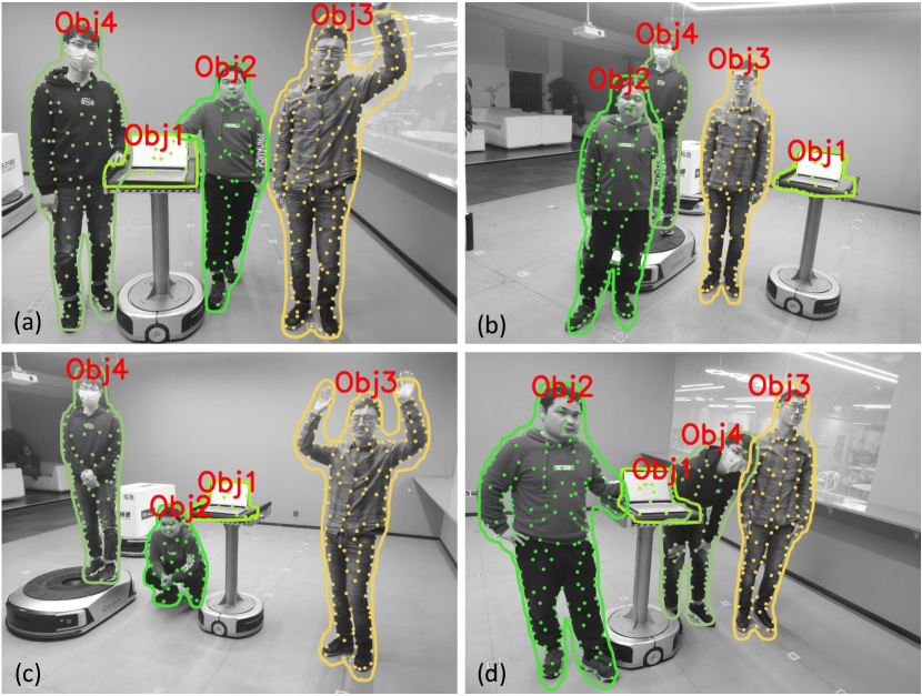
Figure 1: An object matching example. Four objects including 1 rigid object (laptop) and 3 non-rigid objects (human) are identified. Our encoding method is insensitive to viewpoint (Obj 1 in (b) and (d)), scaling (Obj 3 and Obj 4), occlusion (Obj 4), and even posture change (Obj 2 and Obj 3).

II Related Work

We will review both object encoding and visual place recognition methods, since some place recognition algorithms can also be applied to object matching. General detection networks such as Mask R-CNN [9] will not be included, since they are difficult to be used for object matching.

II-A Handcrafted Feature-based Methods

Fast appearance-based mapping (FABMAP) [10] is one of the most classic approaches on handcrafted features. The authors train a visual vocabulary of SURF feature [11] using hierarchical k-means clustering to discretize the high dimensional representation, and then the offline trained visual vocabulary can be used to match features to identify revisited objects. Furthermore, DBoW2 [12] follows this idea and employs ORB binary descriptor [13] to achieve a faster speed. In [14], a dynamic island algorithm is proposed to maintain the vocabulary by grouping similar images, in which repetitive registration of the same descriptor across multiple frames is able to be identified. The strategy of removing redundant descriptors can keep the database at a small scale.

Schlegel et al. [15] introduce an online trained Hamming distance embedded binary search tree (HBST) for image retrieval, which is much faster than traditional FLANN matching methods. However, due to the use of raw descriptors to build the incremental visual vocabulary tree, its memory cost is huge. Reducing the dimension of local features is also an alternative solution. Inspired by the image encoding methods, Carrasco et al. [16] apply hash coding to the local features array, which makes the features extracted from a single image more compact. Gehrig et al. [17] reduce the dimension of BRISK [18] feature with principal component analysis (PCA). They directly employ k-nearest neighbor (K-NN) search on projected descriptors, which makes the query speed several milliseconds faster than searching on pre-trained visual vocabulary. However, those methods are based on handcrafted feature extraction, which is not robust enough when the environment is changed [7].

Tsintotas et al. [19] adopt a dynamic quantization strategy to train the feature online, in which a growing neural gas [20] network is applied. To utilize both structural and visual information, Stumm et al. introduce covisibility graph to represent visual observations [21]. To jointly consider external information, Schlegel et al. embed continuous and selector cues by augmenting each feature descriptor with a binary string [22]. The feature-based methods perform not well when the descriptors are not discriminative enough [23], hence we argue that an object-level place recognition is necessary.

II-B Deep Feature-based Methods

Convolutional neural network (CNN) has made great progress in many computer vision tasks and this triggers another research trend [24]. For example, Z. Chen et al. [25] introduce a multi-scale feature encoding method, in which two CNN architectures are trained and generate features. The viewpoint invariant features provide a huge performance boost. Relja et al. propose NetVLAD [26], in which the authors train a convolutional neural network to replace the parameters of the vector of locally aggregated descriptors (VLAD). Instead of relying on a single method, Hausler et al. [27] combine multiple methods of image processing for visual place recognition, including the sum of absolute difference, histogram of oriented gradients (HOG) [28], spatial Max pooling, and spatial Arg-Max pooling.

To overcome the problem of training data deficiency and multi-modality input dissimilarity, an RGB-D object recognition framework is proposed to effectively embed depth and point cloud data into the RGB domain [29]. Zaki et al. incorporated depth information into a transferred CNN model from image recognition by rendering objects from a canonical perspective and colorizing the depth channel according to distance from the object center [30]. HP-CNN [31] presents a multi-scale object feature representation based on a multi-view 3D object pose using RGB-D sensors.

Our object encoding method is established on deep feature points and descriptors, which has received increasing attention recently. For example, SuperPoint [6] proposes a self-supervised framework for training interest point detectors and descriptors. SuperGlue [7] introduces a graph attention model for feature matching. Intuitively, the interest points and their descriptors form a large fully connected temporally growing graph, in which the feature points are nodes, and their associated descriptors are the node features.

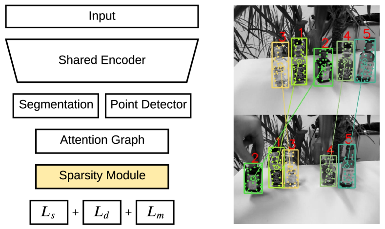
Figure 2: The network structure of AirCode and an example of object matching from the OTB dataset. The detailed structure of the sparsity module is presented in Fig. 3.

III Methodology

III-A Network Structure

As shown in Fig. 2, we propose a simple yet effective framework, AirCode, for object encoding. For each image, we first segment/detect objects and get the feature points on each object. To achieve this, we adopt two off-the-shelf headers with a shared backbone (VGG-16 [32]), i.e., a segmentation header (Mask R-CNN [9]) for object detection/segmentation and a point detector (SuperPoint [6]) for points extraction.

We then take each object as a fully connected graph, where the nodes are the feature points on that object. Assume that there are $M$ key-points on an object, where each point is denoted as its position $\mathbf{p}_{i}=(x,y)$ and associated descriptor $\mathbf{d}_{i}\in\mathbb{R}^{N_{p}}$ ($i\in[1,M]$), where $N_{p}$ is the dimension of the point descriptor. Our goal is to generate an object descriptor $\mathbf{D}_{k}\in\mathbb{R}^{N_{o}}$ for robust object matching based on the object key-points, where $N_{o}$ ($N_{o}>N_{p}$) is the dimension of the object descriptor. For simplicity, we skip the details of the segmentation header and point detector, which are pre-trained models. Instead, we present the sparsity module and loss functions including sparse loss $L_{s}$, dense loss $L_{d}$, and matching loss $L_{m}$.

III-B Graph Embedding with Sparse Node Features

III-B1 Motivation

Inspired by the fact that humans can easily identify an object by recognizing both local distinctive features and global structure [33], we believe that a robust object encoding method should have the following properties: (I) An object descriptor should be able to encode both the local key-point features and the global structural information; (II) The object descriptor should not be significantly affected when a key-point is added or removed, resulting in the insensitivity to viewpoint changes and object deformation.

Therefore, we argue that if only specific positions of the object descriptor can be affected by a key-point (in other words, a key-point has a sparse effect on its object descriptor), then we will be able to obtain a viewpoint invariant object encoding method. This inspires us to formulate the object encoding as a problem of graph sparse embedding.

III-B2 Attention Graph

To encode the local pattern and global structural information simultaneously, we first encode node features $\mathbf{x}_{i}$ for each point as the concatenation of the point positions $\mathbf{p}_{i}$ and descriptor $\mathbf{d}_{i}$, so that

$$\mathbf{x}_{i}=[\mathbf{d}_{i}||\operatorname{MLP}(\mathbf{p}_{i})],\quad\mathbf{x}_{i}\in\mathbb{R}^{N_{n}},$$ (1)

where $N_{n}=N_{p}+N_{m}$, $||$ is the concatenation operator, $\operatorname{MLP}:\mathbb{R}^{2}\mapsto\mathbb{R}^{N_{m}}$ is a multi-layer perceptron module. In practice, the position $\mathbf{p}_{i}$ is normalized to $[-1,1]$ by the object size, which takes the object center as the origin.

We assume that each object is a fully connected graph, where the edge connection weights are learned from an attention mechanism [34]. Specifically, the edge weight $\alpha_{ij}$ between node $\mathbf{x}_{i}$ and node $\mathbf{x}_{j}$ is given as:

$$\mathbf{\alpha}_{ij} =\mathbf{q}_{i}^{\mathsf{T}}\cdot\mathbf{k}_{j},$$ (2a)

$$\mathbf{q}_{i} =\mathbf{W}_{1}\cdot\mathbf{x}_{i}+\mathbf{b}_{1},$$ (2b)

$$\mathbf{k}_{j} =\mathbf{W}_{2}\cdot\mathbf{x}_{j}+\mathbf{b}_{2},$$ (2c)

where $\mathbf{W}_{1}$, $\mathbf{W}_{2}$, $\mathbf{b}_{1}$, and $\mathbf{b}_{2}$ are learnable parameters, which are adopted from the graph attention module in [7]. This encodes the object structure into the node embedding. We refer to [35] for more details about the graph attention network.

III-B3 Sparsity Layer

Inspired by the (II) property mentioned in Section III-B1, we argue that a key-point feature should only be able to affect the object descriptor on its sparse locations, so that the key-points can be added or removed without significantly changing the object descriptor. Therefore, to fully utilize the expressive power, key-points with different local patterns should be written into distinctive locations in the object descriptor. Therefore, the sparse locations should be learned from the contents of the node embeddings. To achieve this, we define two branches for the sparsity layer in (3) for the location and content features, respectively.

$$^{(l+1)}\mathbf{x}_{i}^{L} =\operatorname{ReLU}(\mathbf{W}_{L}^{(l)}\cdot^{(l)}\mathbf{x}_{i}^{L}),$$ (3a)

$${}^{(l+1)}\mathbf{x}_{i}^{C} =\operatorname{ReLU}(\mathbf{W}_{C}^{(l)}\cdot^{(l)}\mathbf{x}_{i}^{C}),$$ (3b)

where the superscript $(l),(l+1)$ indicates their layer number, $\mathbf{W}_{L}^{(l)},\mathbf{W}_{C}^{(l)}\in\mathbb{R}^{N_{o}\times N_{n}^{l}}$ ($N_{n}^{l}<N_{o})$ are the learnable location and content weights, respectively. We set the input of (3) as the same, i.e., ${}^{(1)}\mathbf{x}_{i}^{L}=^{(1)}\mathbf{x}_{i}^{C}$, which is the node embedding from the attention graph. Specifically, each of the two branches has two independent layers. We present a more detailed structure for the proposed sparsity module in Fig. 3.

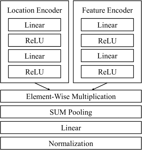
Figure 3: The structure of sparsity module, containing two parallel branches for location and content features, respectively.

Intuitively, if the location feature $\mathbf{x}_{i}^{L}$ is a sparse vector that only a few locations are non-zeros, an object descriptor $\mathbf{D}_{k}$ in (4) will be insensitive to the change of key-points.

$$\mathbf{D}_{k}=\phi({\mathbf{W}_{o}}\sum_{i=1}^{M}\mathbf{x}_{i}^{L}\odot\mathbf{x}_{i}^{C}+\mathbf{b}_{o}),$$ (4)

where $\mathbf{W}_{O}$, $\mathbf{b}_{O}$ are learnable parameters and the operator $\odot$ is an element-wise multiplication. Note that the summation in (4) is a symmetric operator, which can ensure the object descriptor $\mathbf{D}_{k}$ to be invariant to the permutation of key-points.

It is intuitive that fewer number of non-zeros in the location feature $\mathbf{x}_{i}^{L}$ means that the object descriptor $\mathbf{D}_{k}$ will be less affected by the key-point $i$. We next show that how can we ensure the sparsity of the location feature $\mathbf{x}_{i}^{L}$.

III-C Loss Functions

III-C1 Sparse Location Loss

We define the sparse location loss $L_{s}$ as the $\ell_{1}$-norm of $\mathbf{x}_{i}^{L}$ to promote the sparsity:

$$L_{s}:=\sum_{i=1}^{M}\left\|\phi({\mathbf{x}}_{i}^{L})\right\|_{1},$$ (5)

where $\phi(\mathbf{x})=\nicefrac{{\mathbf{x}}}{{\left\|\mathbf{x}\right\|_{2}}}$ is a $\ell_{2}$-normalization function, which is to prevent the location feature from being zero. The $\ell_{1}$ loss for promoting vector sparsity has been widely used in sparse coding for dictionary learning [36]. An intuitive geometric explanation in 2-D space is that the points located on the intersection of axes and unit circle has the minimum $\ell_{1}$-norm, which means that some coordinates tend to be zero.

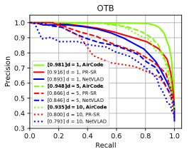
(a) PRC on OTB dataset.

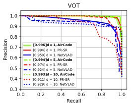
(b) PRC on VOT dataset.

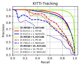
(c) PRC on KITTI Tracking dataset.

Figure 4: The precision-recall curves (PRC) on object matching. The area under curves are shown in the [brackets].

III-C2 Dense Feature Loss

The location sparse loss ensures that the key-point descriptors are encoded into sparse locations in the object descriptor. On the other hand, we also expect that distinctive key-point features are able to cover different locations, which can maximize the location utilization rate of the object descriptor, otherwise the location weights $\mathbf{W}_{L}$ may simply learn to map all key-points to the same sparse locations, which is not expected. Therefore, we define an object dense loss $L_{d}$ as the negative $\ell_{1}$-norm of the summed location features to improve the density of the object descriptor.

$$L_{d}:=\max\left(0,\delta-\phi\left(\left\|\sum^{M}_{i=1}\mathbf{x}_{i}^{L}\right\|_{1}\right)\right),$$ (6)

where $\delta>0$ is a positive constant. A major difference of dense loss (6) from sparse loss (5) is that the summation operator is inside of the $\ell_{1}$-norm, while the $\ell_{2}$-normalization function $\phi$ is outside of the $\ell_{1}$-norm. Intuitively, by optimizing the two loss functions simultaneously, we are able to push the key-point location features to be sparse, while retaining the density of object descriptor, so that similar key-points will share similar locations, while distinctive key-points tend to cover different locations. This means that the object descriptor is insensitive to the changes of key-points, resulting in the invariance to viewpoint changes and object deformation.

Note that the sparsity in this paper is different from the traditional sparse coding techniques [36] and deep sparse coding network [37] which are to learn a dictionary and minimize a reconstruction error, while ours is to learn sparse features without any approximation and dictionary. It is also different from the model compression networks such as [38], which are to learn sparse convolutional weights, as we have no sparse constraints on the learnable weights $\mathbf{W}_{L}$.

III-C3 Object Matching Loss

The object matching loss $L_{m}$ maximizes the cosine similarity for positive object pairs and minimizes the cosine similarity for negative pairs.

$$L_{m}:= \sum_{\{p,q\}\in P^{+}}(1-S\left(\mathbf{D}_{p},\mathbf{D}_{q}\right))$$ (7)

$$+ \sum_{\{p,q\}\in P^{-}}\max(0,S(\mathbf{D}_{p},\mathbf{D}_{q})-\zeta),$$

where $\zeta=0.2$ is a constant margin, $S$ is the cosine similarity, and $P^{+}$/$P^{-}$ are positive/negative object pairs, respectively.

IV Experiments

IV-A Implementation Details and Baseline

We take pre-trained backbone CNN and key-point detector from SuperPoint [6], pre-trained segmentation header from Mask R-CNN [9], and train the graph and sparsity modules only on COCO dataset [39]. Random homographies are generated for data augmentation, including the perspective, translation, rotation, and scale transforms. We take a batch size of 16, a learning rate of $10^{-5}$, and the RMSprop [40] optimizer for training AirCode. In the experiments, we set $N_{p}=256$, $N_{m}=16$, and $N_{o}=2048$. We set the loss weights as 1.0, 0.5, 0.1, and 10 for negative matching, positive matching, sparse, and dense loss functions, respectively. The source code and pretrained models are available at https://github.com/wang-chen/AirCode.

We note that an attention graph is also used in SuperGlue [7] to match feature points. It broadcasts node features from two images for point matching, while object embedding in AirCode is self-representative thus the node features can only be propagated within the object. Therefore, we don’t take the point features from SuperGlue as our inputs, since we expect that an object descriptor doesn’t use information from external images, so that one query descriptor can be matched to objects in database without exchanging information.

We perform extensive comparison with the state-of-the-art methods including NetVLAD [26] and PR-SR [3]. NetVLAD is an image matching method and has been adopted by many place recognition algorithms, e.g., [41, 42], which verifies its generalization ability. In the experiments, we use it as a feature aggregation method. PR-SR applied a saliency detection technique to segment objects, which sometimes is not able to detect all objects. For fair comparison, we provide the ground truth mask of object segmentation for PR-SR and only compare with its object matching performance.

IV-B Object Matching

We first present the performance of the proposed method on object matching. Three datasets will be tested extensively, including OTB-2013 [43], VOT-2016 [44], and KITTI Tracking [45]. Note that we present performance on tracking datasets but don’t compare with tracking methods such as [46], as they mainly use the information from consecutive frames, while we extract descriptors for matching with any frames. The performance is reported without finetuning on these datasets.

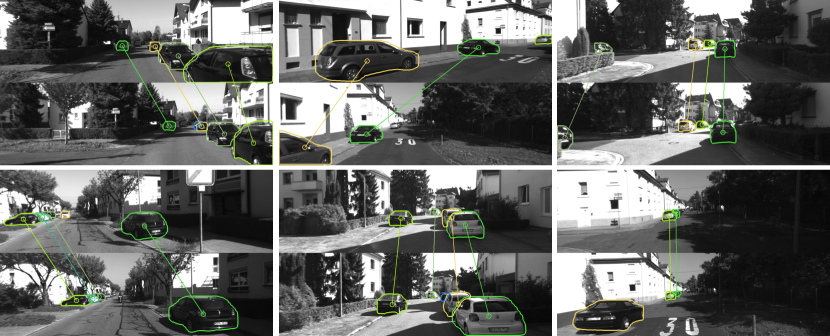
Figure 5: The examples of car matching in the KITTI Odometry dataset. Although all the cars look similar, AirCode is still able to correctly identify the same cars from different viewpoints.

TABLE I: Object Matching on the OTB dataset.

	Method	Precision	Recall	F1
$d=1$	NetVLAD	78.5	83.0	80.7
	PR-SR	82.7	89.3	85.9
	AirCode	93.2	92.6	92.9
$d=3$	NetVLAD	72.7	79.7	76.0
	PR-SR	81.7	79.1	80.4
	AirCode	88.3	86.4	87.3
$d=5$	NetVLAD	74.0	81.0	77.3
	PR-SR	81.0	73.2	76.9
	AirCode	87.6	86.2	86.9
$d=10$	NetVLAD	70.2	80.7	75.1
	PR-SR	71.1	72.2	71.6
	AirCode	85.6	84.7	85.1

IV-B1 OTB Dataset

We select all sequences of OTB in which objects have labels in the COCO dataset and contain 5 or more key-points. To test the robustness, we report the matching performance for frame pairs that have $d-1$ ($d>1$) frames in between. Intuitively, matching is more difficult for larger $d$ and object tracking is the case of $d=1$. We take an object pair as a match if their cosine similarity is larger than a threshold $\delta$. The overall performance of precision, recall, and F1-score is presented in Table I. It can be seen that AirCode outperforms NetVLAD with a large margin of 5%-15% and outperforms PR-SR by a margin of 3%-10%.

Intuitively, the precision-recall curves (PRC) can be obtained for each sequence by changing the threshold $\delta$. Fig. 4a shows the PRC for all datasets, in which the areas under precision-recall curves (AU-PRC) are reported in the brackets. AirCode achieves a much higher performance for all cases, i.e., an average higher performance of 8.8%, 10.2%, and 14.2% than NetVLAD and 6.5%, 8.2%, and 13.5% than PR-SR for $d=1$, $5$, and $10$, respectively. We notice that the performance of AirCode decreases much slower with increasing $d$ than other methods, which verifies its robustness.

TABLE II: Object Matching on the VOT dataset.

	Method	Precision	Recall	F1
$d=1$	NetVLAD	90.9	88.7	89.8
	PR-SR	98.3	95.1	96.7
	AirCode	98.6	98.3	98.4
$d=3$	NetVLAD	90.0	92.1	91.0
	PR-SR	97.2	94.2	95.7
	AirCode	97.4	98.2	97.8
$d=5$	NetVLAD	89.5	90.4	89.9
	PR-SR	90.3	90.4	90.3
	AirCode	95.8	95.9	95.8
$d=10$	NetVLAD	90.0	90.5	90.2
	PR-SR	77.9	85.1	81.3
	AirCode	95.6	95.3	95.4

IV-B2 VOT Dataset

The VOT dataset mainly contains blurred and non-rigid objects such as humans. The overall performance is presented in Table II, in which we achieve a higher performance of 1-5% than NetVLAD and comparable performance with PR-SR. The PRC performance is reported in Fig. 4b, in which we achieve a higher performance of 4.6%, 7.0%, and 6.4%, for $d=1$, $5$, and $10$ than NetVLAD and 0.2%, 2.0%, and 8.2% than PR-SR for $d=1$, $5$, and $10$, respectively.s.

IV-B3 KITTI Tracking

The KITTI Tracking is a multi-object tracking dataset [45], thus we calculate the similarity of all object pairs in each frame pair. The overall performance on precision, recall, and F1-score are reported in Table III in which AirCode still achieves the best performance. Their PRC are shown in Fig. 4c, in which we achieve a higher performance of 7.2%, 14.7%, and 15.6% than NetVLAD and 6.1%, 7.5%, and 1.2% than PR-SR for $d=1$, $5$, and $10$, respectively.

TABLE III: Object Matching on the KITTI Tracking dataset.

	Method	Precision	Recall	F1
$d=1$	NetVLAD	82.6	84.4	83.5
	PR-SR	82.0	84.3	83.1
	AirCode	93.8	93.0	93.4
$d=3$	NetVLAD	72.7	74.1	73.4
	PR-SR	79.4	74.5	76.9
	AirCode	89.1	85.8	87.4
$d=5$	NetVLAD	68.6	68.8	68.7
	PR-SR	78.5	70.4	74.2
	AirCode	82.3	80.6	81.4
$d=10$	NetVLAD	57.4	65.3	61.1
	PR-SR	71.4	69.3	70.3
	AirCode	71.0	69.9	70.4

IV-C Semantic Relocalization

To further verify its robustness, we apply the proposed method to semantic relocalization, which will be evaluated on the KITTI Odometry dataset [23]. We select the sequences with significant loop closures, i.e., ’00’, ’05’, and ’06’. To calculate the similarity of two images, we accumulate the similarities of all the object pairs whose similarities are larger than a threshold. To test the robustness of our method, we mainly re-identify cars for relocalization, which is much more difficult than matching distinct objects. Although the overall performance of relocalization will be slightly harmed, such a setting is able to verify the robustness of the object descriptor, as the cars on the road in KITTI datasets are very similar thus the performance on car matching is more convincing.

TABLE IV: Semantic Relocalization on KITTI Odometry.

Sequence	Method	Precision	Recall	F1
00	NetVLAD	21.1	41.3	27.9
	AirCode	95.7	75.4	84.3
05	NetVLAD	19.0	25.3	21.7
	AirCode	97.2	40.1	56.8
06	NetVLAD	39.0	27.4	32.2
	AirCode	95.4	47.7	63.6

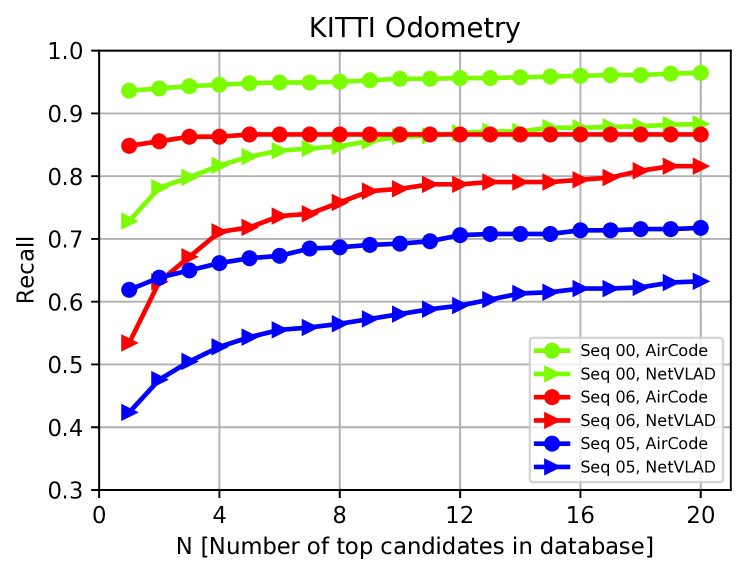
Figure 6: The performance of semantic re-localization.

The overall performance is listed in Table IV, in which we can see that we achieve more reliable performance than NetVLAD for all sequences. Note that we remove assistant techniques such as geometric verification [3] to ensure that the improvements come from the proposed object descriptor. We also present the recall curves in Fig. 6, in which we accept the top $N$ pairs as a re-localization. It can be seen that, $\forall N$, $N\in[1,20]$, we are able to achieve better performance with a large margin than NetVLAD for all sequences, which verifies the effectiveness of AirCode. PR-SR is excluded from this task, since it computes correlation for all object pairs, which is quite computationally heavy.

IV-D Live Demo & Limitation

In this section, we present a live demo to demonstrate the generalization ability and robustness of the proposed method. In this demo, we still use the pre-trained model mentioned in Section IV-B without any fine-tuning. It can be seen that, compared to NetVLAD, AirCode is quite robust to the change of viewpoint in Fig. 7a, object occlusion in Fig. 7b, and object deformation in Fig. 7c and 7d. For better visualization, we strongly suggest the readers watch the video attached to this paper at https://youtu.be/ZhW4Qk1tLNQ.

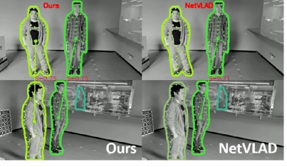
(a) Change of Viewpoint.

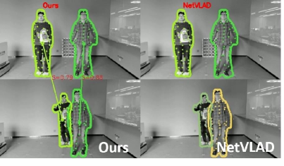
(b) Object Occlusion.

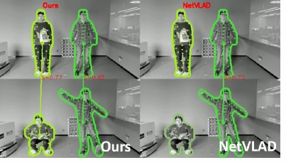
(c) Object Deformation I.

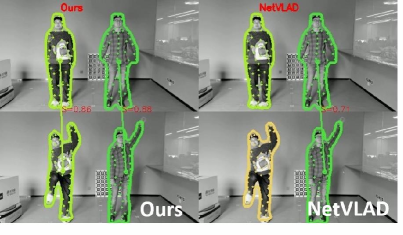
(d) Object Deformation II.

Figure 7: The live object matching demo.

IV-E Sparsity Analysis

We provide the sparsity analysis for the proposed method based on COCO dataset [39]. The distribution of non-zero locations of the key-point features is shown in Fig. 8a, in which we can see that only 700-800 out of 2048 locations are non-zeros. This verifies the objective of sparse loss in (5). The statistics of non-zero locations of the object descriptor are presented in Fig. 8b. As expected, the non-zero locations increase with the number of key-points detected in the object, which also verifies the objective of dense loss (6).

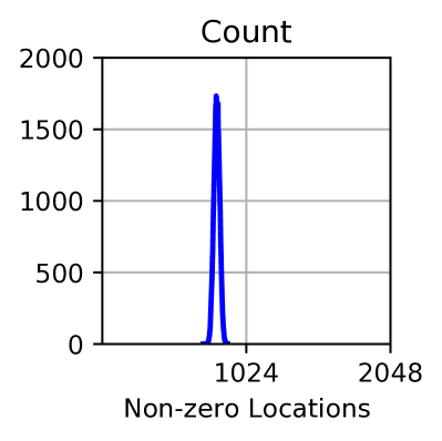
(a) Key-point Sparsity.

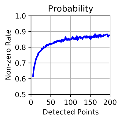
(b) Average Object Denseness

Figure 8: The statistics of feature sparsity.

Note that we expect to group similar key-points into the same locations as in (3a), so that the location of a single object descriptor will not be quickly used up by simply increasing the number of key-points, since an object typically cannot cover all different points. This can be further verified by calculating the location usage over different object descriptors. To this end, we randomly select $N$ images and calculate how often each location of the object descriptor is used. We list the usage rate for $N=1$, $10$, $100$, $1000$, and $10000$ in Table V. It can be seen that the location of object descriptor is nearly fully used by increasing the number of objects, which further verifies the effectiveness of the dense feature loss.

TABLE V: The Location Usage of Object Descriptors.

N	1	10	100	1000	10000
Usage Rate	0.868	0.927	0.966	0.979	0.984

IV-F Efficiency

This section presents the runtime of the proposed modules, which are listed in Table VI. It can be seen that the sparsity layer only takes about 1 m s , which is much lower than the graph attention network used in this module. The overall running time is about 9.3 m s , which satisfies the real-time requirements of most robotic applications.

TABLE VI: Runtime Analysis.

Module	Node Encoding	Graph	Sparsity	Overall
Time	0.847 m s	7.302 m s	1.131 m s	9.280 m s

V Ablation Study

V-A Sparsity Module

To analyze the effectiveness of the sparsity module, we compare with a model by replacing it with a fully connected layer to output a descriptor with the same dimension as the original one. Similar to Section IV-B and Section IV-C, the performance on object matching ($d=10$) and semantic relocalization are evaluated. The results are listed in the 2nd and 4th row of Table VII and Table VIII, respectively, where “w/o sparsity” denotes the model without sparsity module. It can be seen that the sparsity layer brings a huge overall performance gain, especially in the task of semantic relocalization. It is also observed that, AirCode w/o sparsity performs a little bit better in object matching on OTB dataset. This is because OTB is relatively an easier dataset, so the model with a fully connected layer can also work well.

TABLE VII: The Ablation Study on Object Matching.

Dataset	OTB	VOT	KITTI Tracking
AirCode${}^{\text{w/o sparsity}}$	94.0	98.6	79.7
AirCode${}^{\text{w/o loss}}$	91.7	98.8	75.1
AirCode	93.5	99.3	80.4

V-B Loss Functions

We next explore that effects of the proposed sparse and dense loss functions in (5) and (6). Note that the two loss functions should be used simultaneously as they need to balance each other, so we remove both of them in this experiment. The 3rd and 4th row of Table VII and Table VIII show that removing the loss functions leads to a significant drop of overall performance in both tasks. In the semantic relocalization experiment, AirCode also achieves an average higher F1-score of 4% than AirCode w/o loss, which verifies the necessity of the proposed sparse and dense loss functions. We notice that AirCode w/o loss has a higher recall. The reason is that every point feature in AirCode is sparser, so the final object encoding is more discriminative, which leads to a higher precision but lower recall with the same threshold.

TABLE VIII: The Ablation Study on Semantic Relocalization.

Metric	Precision	Recall	F1
AirCode${}^{\text{w/o sparsity}}$	90.3	37.1	52.6
AirCode${}^{\text{w/o loss}}$	76.4	57.2	65.4
AirCode	96.0	54.4	69.4

VI Limitation

Despite the promising prospect and outstanding performance, AirCode still has several limitations. First, its robustness depends on the performance of pre-trained segmentation header and point detector, thus its performance may not be stable when objects are segmented or the feature points are detected incorrectly. Second, the object categories also depend on the object detector, thus it is difficult for AirCode to match novel objects. Third, with robot moving, we often observe an object from multiple viewpoints, while AirCode is designed for object encoding on a single image. Therefore, it can be further improved by introducing temporally “evolving” object representation, which will be taken as our future work.

VII Conclusion

In this work, we present a novel object encoding method, which can be used in many robotic tasks such as autonomous exploration and semantic relocalization. To be robust to the number of key-points detected, we propose a sparse encoding method to ensure that each key-point can only affect a small part of the object descriptors, making the global descriptors robust in severe conditions such as viewpoint changes and object deformation. In the experiments, we show that it achieves superior performance in object matching and provides reliable semantic relocalization. We also show a live demo to demonstrate its robustness. We expect that this method will play an important role in robotic applications.

References

- [1] C. Wang, W. Wang, Y. Qiu, Y. Hu, and S. Scherer, “Visual memorability for robotic interestingness via unsupervised online learning,” in Computer Vision–ECCV 2020: 16th European Conference, Glasgow, UK, August 23–28, 2020, Proceedings, Part II 16. Springer, 2020, pp. 52–68.
- [2] C. Wang, Y. Qiu, W. Wang, Y. Hu, S. Kim, and S. Scherer, “Unsupervised online learning for robotic interestingness with visual memory,” IEEE Transactions on Robotics, 2021.
- [3] H. Wang, C. Wang, and L. Xie, “Online visual place recognition via saliency re-identification,” in IEEE/RSJ International Conference on Intelligent Robots and Systems (IROS), 2020.
- [4] M.-P. Dubuisson and A. K. Jain, “A modified hausdorff distance for object matching,” in Proceedings of 12th international conference on pattern recognition, vol. 1. IEEE, 1994, pp. 566–568.
- [5] R. Mur-Artal and J. D. Tardós, “Orb-slam2: An open-source slam system for monocular, stereo, and rgb-d cameras,” IEEE Transactions on Robotics, vol. 33, no. 5, pp. 1255–1262, 2017.
- [6] D. DeTone, T. Malisiewicz, and A. Rabinovich, “Superpoint: Self-supervised interest point detection and description,” in Proceedings of the IEEE conference on computer vision and pattern recognition workshops, 2018, pp. 224–236.
- [7] P.-E. Sarlin, D. DeTone, T. Malisiewicz, and A. Rabinovich, “Superglue: Learning feature matching with graph neural networks,” in Proceedings of the IEEE/CVF conference on computer vision and pattern recognition, 2020, pp. 4938–4947.
- [8] C. Wang, Y. Qiu, D. Gao, and S. Scherer, “Lifelong graph learning,” arXiv preprint arXiv:2009.00647, 2021.
- [9] K. He, G. Gkioxari, P. Dollár, and R. Girshick, “Mask r-cnn,” in Proceedings of the IEEE international conference on computer vision, 2017, pp. 2961–2969.
- [10] A. Glover, W. Maddern, M. Warren, S. Reid, M. Milford, and G. Wyeth, “Openfabmap: An open source toolbox for appearance-based loop closure detection,” in Robotics and automation (ICRA), 2012 IEEE international conference on. IEEE, 2012, pp. 4730–4735.
- [11] H. Bay, T. Tuytelaars, and L. Van Gool, “Surf: Speeded up robust features,” in European conference on computer vision. Springer, 2006, pp. 404–417.
- [12] D. Gálvez-López and J. D. Tardos, “Bags of binary words for fast place recognition in image sequences,” IEEE Transactions on Robotics, vol. 28, no. 5, pp. 1188–1197, 2012.
- [13] E. Rublee, V. Rabaud, K. Konolige, and G. Bradski, “Orb: An efficient alternative to sift or surf,” in Computer Vision (ICCV), 2011 IEEE international conference on. IEEE, 2011, pp. 2564–2571.
- [14] E. Garcia-Fidalgo and A. Ortiz, “ibow-lcd: An appearance-based loop-closure detection approach using incremental bags of binary words,” IEEE Robotics and Automation Letters, vol. 3, no. 4, pp. 3051–3057, 2018.
- [15] D. Schlegel and G. Grisetti, “HBST: A hamming distance embedding binary search tree for feature-based visual place recognition,” IEEE Robotics and Automation Letters, vol. 3, no. 4, pp. 3741–3748, 2018.
- [16] P. L. N. Carrasco, F. Bonin-Font, and G. Oliver-Codina, “Global image signature for visual loop-closure detection,” Autonomous Robots, vol. 40, no. 8, pp. 1403–1417, 2016.
- [17] M. Gehrig, E. Stumm, T. Hinzmann, and R. Siegwart, “Visual place recognition with probabilistic voting,” in 2017 IEEE International Conference on Robotics and Automation (ICRA). IEEE, 2017, pp. 3192–3199.
- [18] S. Leutenegger, M. Chli, and R. Siegwart, “Brisk: Binary robust invariant scalable keypoints,” in 2011 IEEE international conference on computer vision (ICCV). Ieee, 2011, pp. 2548–2555.
- [19] K. A. Tsintotas, L. Bampis, and A. Gasteratos, “Assigning visual words to places for loop closure detection,” in 2018 IEEE International Conference on Robotics and Automation (ICRA). IEEE, 2018, pp. 5979–5985.
- [20] B. Fritzke, “A growing neural gas network learns topologies,” in Advances in neural information processing systems, 1995, pp. 625–632.
- [21] E. Stumm, C. Mei, S. Lacroix, J. Nieto, M. Hutter, and R. Siegwart, “Robust visual place recognition with graph kernels,” in Proceedings of the IEEE Conference on Computer Vision and Pattern Recognition, 2016, pp. 4535–4544.
- [22] D. Schlegel and G. Grisetti, “Adding cues to binary feature descriptors for visual place recognition,” in 2019 International Conference on Robotics and Automation (ICRA). IEEE, 2019, pp. 5488–5494.
- [23] A. Geiger, P. Lenz, and R. Urtasun, “Are we ready for autonomous driving? the kitti vision benchmark suite,” in 2012 IEEE conference on computer vision and pattern recognition. IEEE, 2012, pp. 3354–3361.
- [24] C. Wang, J. Yang, L. Xie, and J. Yuan, “Kervolutional neural networks,” in The IEEE Conference on Computer Vision and Pattern Recognition (CVPR), 2019, pp. 31–40.
- [25] Z. Chen, A. Jacobson, N. Sünderhauf, B. Upcroft, L. Liu, C. Shen, I. Reid, and M. Milford, “Deep learning features at scale for visual place recognition,” in 2017 IEEE International Conference on Robotics and Automation (ICRA). IEEE, 2017, pp. 3223–3230.
- [26] R. Arandjelovic, P. Gronat, A. Torii, T. Pajdla, and J. Sivic, “Netvlad: Cnn architecture for weakly supervised place recognition,” in Proceedings of the IEEE conference on computer vision and pattern recognition, 2016, pp. 5297–5307.
- [27] S. Hausler, A. Jacobson, and M. Milford, “Multi-process fusion: Visual place recognition using multiple image processing methods,” IEEE Robotics and Automation Letters, vol. 4, no. 2, pp. 1924–1931, 2019.
- [28] N. Dalal and B. Triggs, “Histograms of oriented gradients for human detection,” in Proceedings of the IEEE Computer Society Conference on Computer Vision and Pattern Recognition (CVPR), 2005.
- [29] H. F. Zaki, F. Shafait, and A. Mian, “Convolutional hypercube pyramid for accurate rgb-d object category and instance recognition,” in 2016 IEEE International Conference on Robotics and Automation (ICRA). IEEE, 2016, pp. 1685–1692.
- [30] M. Schwarz, H. Schulz, and S. Behnke, “Rgb-d object recognition and pose estimation based on pre-trained convolutional neural network features,” in 2015 IEEE international conference on robotics and automation (ICRA). IEEE, 2015, pp. 1329–1335.
- [31] H. F. Zaki, F. Shafait, and A. Mian, “Viewpoint invariant semantic object and scene categorization with rgb-d sensors,” Autonomous Robots, vol. 43, no. 4, pp. 1005–1022, 2019.
- [32] K. Simonyan and A. Zisserman, “Very deep convolutional networks for large-scale image recognition,” arXiv:1409.1556, 2014.
- [33] M. J. Tarr and W. G. Hayward, “The concurrent encoding of viewpoint-invariant and viewpoint-dependent information in visual object recognition,” Visual Cognition, vol. 25, pp. 100–121, 2017.
- [34] A. Vaswani, N. Shazeer, N. Parmar, J. Uszkoreit, L. Jones, A. N. Gomez, Ł. Kaiser, and I. Polosukhin, “Attention is all you need,” in Advances in neural information processing systems, 2017, pp. 5998–6008.
- [35] P. Veličković, G. Cucurull, A. Casanova, A. Romero, P. Liò, and Y. Bengio, “Graph Attention Networks,” International Conference on Learning Representations (ICLR), 2018.
- [36] H. Lee, A. Battle, R. Raina, and A. Y. Ng, “Efficient sparse coding algorithms,” in Advances in neural information processing systems. Citeseer, 2007, pp. 801–808.
- [37] Y. Gwon, M. Cha, and H. Kung, “Deep sparse-coded network (dsn),” in 2016 23rd International Conference on Pattern Recognition (ICPR). IEEE, 2016, pp. 2610–2615.
- [38] X. Liu, W. Li, J. Huo, L. Yao, and Y. Gao, “Layerwise sparse coding for pruned deep neural networks with extreme compression ratio,” in Proceedings of the AAAI Conference on Artificial Intelligence, vol. 34, no. 04, 2020, pp. 4900–4907.
- [39] T.-Y. Lin, M. Maire, S. Belongie, J. Hays, P. Perona, D. Ramanan, P. Dollár, and C. L. Zitnick, “Microsoft coco: Common objects in context,” in European conference on computer vision. Springer, 2014, pp. 740–755.
- [40] G. Hinton, N. Srivastava, and K. Swersky, “Neural networks for machine learning lecture 6a overview of mini-batch gradient descent,” Cited on, vol. 14, no. 8, 2012.
- [41] P.-E. Sarlin, C. Cadena, R. Siegwart, and M. Dymczyk, “From coarse to fine: Robust hierarchical localization at large scale,” in Proceedings of the IEEE/CVF Conference on Computer Vision and Pattern Recognition, 2019, pp. 12 716–12 725.
- [42] Z. Liu, S. Zhou, C. Suo, P. Yin, W. Chen, H. Wang, H. Li, and Y.-H. Liu, “Lpd-net: 3d point cloud learning for large-scale place recognition and environment analysis,” in Proceedings of the IEEE/CVF International Conference on Computer Vision, 2019, pp. 2831–2840.
- [43] Y. Wu, J. Lim, and M.-H. Yang, “Online object tracking: A benchmark,” in Proceedings of the IEEE conference on computer vision and pattern recognition, 2013, pp. 2411–2418.
- [44] M. Kristan, J. Matas, A. Leonardis, T. Vojir, R. Pflugfelder, G. Fernandez, G. Nebehay, F. Porikli, and L. Čehovin, “A novel performance evaluation methodology for single-target trackers,” IEEE Transactions on Pattern Analysis and Machine Intelligence, vol. 38, no. 11, pp. 2137–2155, Nov 2016.
- [45] J. Luiten, A. Osep, P. Dendorfer, P. Torr, A. Geiger, L. Leal-Taixé, and B. Leibe, “Hota: A higher order metric for evaluating multi-object tracking,” International journal of computer vision, vol. 129, Oct.2020.
- [46] C. Wang, L. Zhang, L. Xie, and J. Yuan, “Kernel cross-correlator,” in Thirty-Second AAAI Conference on Artificial Intelligence (AAAI), 2018, pp. 4179–4186.