Do alcoved lattice polytopes have unimodal $h^{*}$-vector?

Abstract.

We show that $h^{*}$-vectors of alcoved polytopes $P\subset\mathbb{R}^{n}$ (of Lie type $\mathcal{A}$) are unimodal if they contain interior lattice points and their facets have lattice distance $1$ to the set of interior lattice points. The maximal possible such distance for general alcoved polytopes is shown to be $\dim(P)-1$. A secondary purpose of the paper is to serve as a guide to previous work surrounding unimodality of $h^{*}$-vectors of alcoved polytopes and related questions.

Introduction

A finite sequence $(s_{1},s_{2},\ldots,s_{n})$ is called unimodal if there exists an index $k\in\{1,\ldots,n\}$ such that $s_{1}\leq\ldots\leq s_{k}\geq\ldots\geq s_{n}$. We are particularly interested in this property for sequences arising from lattice polytopes, which are polytopes in $\mathbb{R}^{n}$ whose vertices lie in $\mathbb{Z}^{n}$, namely $h^{*}$-vectors. Closely related (at least in our case) are face vectors of (regular unimodular) triangulations, namely $h$-vectors. There is a variety of conjectures and theorems about the unimodality of $h$-vectors and $h^{*}$-vectors of different objects. The articles [34] by Stanley, [10] by Brenti, and [8] by Brändén are excellent surveys on unimodality in combinatorics. We focus particularly on unimodality in Ehrhart theory for which we refer to the survey [9] by Braun.

The $h^{*}$-polynomial of a lattice polytope is derived from its Ehrhart series. For $t\in\mathbb{N}$, write $L_{P}(t)=|(tP)\cap\mathbb{Z}^{n}|$ for the number of lattice points in the dilate $tP$ of the lattice polytope $P\subset\mathbb{R}^{n}$. Its Ehrhart series is the generating function of this lattice count, i.e.

$$\operatorname{Ehr}_{P}(z)=1+\sum_{t\geq 1}L_{P}(t)z^{t}.$$

It turns out that this series is actually a rational function with denominator $(1-z)^{d+1}$, where $d$ is the dimension of $P$. The numerator is a polynomial of degree at most $d$ and its coefficient vector is the $h^{*}$-polynomial of $P$, more precisely

$$\operatorname{Ehr}_{P}(z)=\frac{h_{d}^{*}z^{d}+h_{d-1}^{*}z^{d-1}+\ldots+h_{1}^{*}z+h_{0}^{*}}{(1-z)^{d+1}}.$$

The $h^{*}$-vector of $P$ is the vector of coefficients of the $h^{*}$-polynomial. We are interested in unimodality of the $h^{*}$-vector.

Our main Theorem 2.1 says that the $h^{*}$-vector is unimodal for a special class of lattice polytopes called alcoved polytopes of Lie type $\mathcal{A}$ whose facets have lattice distance $1$ to the interior lattice points. We define these notions in Section 1. We also show that our proof strategy does not work if we drop the assumption about the lattice distance in 2.6. Along the way, we show Theorem 2.2 stating that the $h^{*}$-vector is unimodal for any $d$-dimensional lattice polytope $P$ that admits a unimodular triangulation $\Delta$ such that the induced simplicial complex on $(\partial P)\cap\mathbb{Z}^{d}$ is a triangulation of $\partial P$.

Here is some historical context of this result with other classes of lattice polytopes with unimodal $h^{*}$-vectors.

Theorem (Hibi [19]).

Reflexive lattice polytopes up to dimension $5$ have unimodal $h^{*}$-vectors.

This theorem does not hold for higher dimensions. Mustaţă and Payne [26, Ex. 1.1], [27, Thm. 1.4] showed that there exist reflexive polytopes (even simplices) of all dimensions greater than $5$ without unimodal $h^{*}$-vectors.

Bruns and Römer showed that if a reflexive (or more generally a Gorenstein) polytope has a regular unimodular triangulation, then its $h^{*}$-vector is unimodal.

Theorem (Bruns & Römer [13]).

Gorenstein lattice polytopes with regular unimodular triangulation have unimodal $h^{*}$-vectors.

It has been conjectured that the property of having a unimodular triangulation can be weakened even more to the more general condition of having the integer decomposition property (IDP).

Conjecture (Hibi & Ohsugi [20]).

A lattice polytope which is Gorenstein and IDP has unimodal $h^{*}$-vector.

Even more generally, there are no known examples of IDP polytopes without unimodal $h^{*}$-vectors. The next question or conjecture is part of a conjecture of Stanley’s that standard graded Cohen–Macaulay integral domains have unimodal $h$-vectors.

Conjecture (Stanley, see [29, Question 1.1]).

IDP polytopes have unimodal $h^{*}$-vectors.

A special class of polytopes that is conjectured to have unimodal $h^{*}$-vectors is the class of order polytopes: Let $P=(\{p_{1},\ldots,p_{n}\},\preccurlyeq)$ be a finite poset. The order polytope $\mathcal{O}(P)\subset\mathbb{R}^{n}$ is defined by the inequalities:

$$0\leq x_{i}\leq 1 \text{ for all }i\in\{1,\ldots,n\},$$

$$x_{i}\leq x_{j} \text{ if }p_{i}\preccurlyeq p_{j}.$$

Order polytopes have regular unimodular triangulations. We will see an example of such a triangulation for the more general class of alcoved polytopes in Definition 1.1.

Alcoved polytopes have regular unimodular triangulations (but they are not necessarily Gorenstein or reflexive). Here is a general result in the direction of unimodality of $h^{*}$-vectors that gives us about half of the inequalities in our main theorem.

Theorem (Hibi & Stanley, see Athanasiadis [3, Theorem 1.3]).

Let $P$ be a $d$-dimensional lattice polytope with a regular unimodular triangulation. Then:

$$\begin{cases}&h^{*}_{i}(P)\geq h^{*}_{d+1-i}(P)\hskip 82.0pt\text{ for }1\leq i\leq\left\lfloor\frac{d+1}{2}\right\rfloor,\\ &h^{*}_{\left\lfloor\frac{d+1}{2}\right\rfloor}(P)\geq\ldots\geq h^{*}_{d-1}(P)\geq h^{*}_{d}(P),\\ &h^{*}_{i}(P)\leq\binom{h^{*}_{1}(P)+i-1}{i}\hskip 80.0pt\text{ for }0\leq i\leq d.\end{cases}$$

1. Preliminaries

We write $[d]$ for the set $\{1,2,\ldots,d\}$.

1.1. Alcoved Polytopes

Definition 1.1.

A hyperplane coming from an affine Coxeter arrangement of type $\mathcal{A}_{d}$ is a hyperplane of the form

$$H_{d}(i,j,k)=\{\begin{pmatrix}y_{1}\\ \vdots\\ y_{d}\end{pmatrix}\in\mathbb{R}^{d}\mid y_{i}-y_{j}=k_{ij}\}$$

for some $k_{ij}\in\mathbb{Z}$, $i,j\in\{0,\ldots,d\}$ and $y_{0}=0$. We will call such hyperplanes alcove hyperplanes.

A $d$-dimensional polyhedron is called an alcoved polyhedron (of Lie type $\mathcal{A}$) if all of its facet-defining hyperplanes are alcove hyperplanes. If $P$ is bounded it is called an alcoved polytope of Lie type $\mathcal{A}$. In the following by an alcoved polytope we always mean an alcoved polytope of Lie type $\mathcal{A}$.

The $\mathcal{H}$-description of an alcoved $d$-polyhedron $P$ with $m$ facets can be written as

$$P=\{x\in\mathbb{R}^{d}\mid Mx\leq b\},$$

for $b\in\mathbb{Z}^{m}$ and where $M$ is an $(m\times d)$-matrix with row vectors $a_{k}\in\{e_{i}\colon i\in[d]\}\cup\{e_{i}-e_{j}\colon i,j\in[d]\}$ for all $k\in\{1,\ldots m\}$. This matrix $M$ is always a totally unimodular matrix, i.e. every minor of $M$ is in $\{0,\pm 1\}$. In particular, this implies that alcoved polytopes are lattice polytopes (see [5, Sect. 7.1]).

We obtain the alcoved triangulation of an alcoved $d$-polytope $P$ by subdividing it by all alcove hyperplanes $H_{d}(i,j,k)$ ($i,j\in\{0\}\cup[d]$, $k\in\mathbb{Z}$), see [23, Section 2.3]. The simplices of the alcoved triangulation are called alcoves. The unimodular triangulation is regular, for example via the lifting function

$$y_{d+1}=\sum_{i=1}^{d}y_{i}^{2}+\sum_{\{i,j\}\in\{1,\ldots,d\}}(y_{i}-y_{j})^{2}.$$

Examples of alcoved polytopes include concrete realizations of hypersimplices and order polytopes (see [23] for more details and more examples of alcoved polytopes).

Example 1.2 (Hypersimplex).

The hypersimplex $\Delta_{d,k}$ is usually defined as the set of vectors $x=(x_{1},x_{2},\ldots,x_{d})$ in $[0,1]^{d}\subset\mathbb{R}^{d}$ whose coordinates sum to $k$, i.e. $\sum_{i=1}^{d}x_{i}=k$. After the affine change of coordinates $z_{j}=\sum_{i=1}^{j}x_{i}$, the hypersimplex can be defined by the inequalities

$$\begin{array}[]{cl}0\leq z_{1}\leq 1&\\ k\leq z_{d}\leq k&\\ 0\leq z_{i}-z_{i-1}\leq 1&\text{ for all }i\in[d]\end{array}$$

in the affine hyperplane $\{z\colon z_{d}=k\}\subset\mathbb{R}^{d}$. This is a description as an alcoved polytope.

Example 1.3 (Order polytopes).

Let $P=(\{p_{1},p_{2},\ldots,p_{n}\},\preceq)$ be a finite poset. The order polytope $\mathcal{O}(P)\subset\mathbb{R}^{d}$ is the polytope defined by the inequalities

$$0\leq x_{i}\leq 1 \text{ for all }i\in[n]$$

$$x_{i}\leq x_{j} \text{ whenever }p_{i}\preceq p_{j}.$$

The order polytope corresponding to an anti-chain is the $0/1$-cube. The order polytope of a chain is a simplex.

Since an alcoved polytope can only have a finite number of admissible facet normals, there exists a unique alcoved polytope of minimal volume among all alcoved polytopes containing the origin in the interior, which we call $Q_{d}$ throughout the paper. This polytope is obtained by taking the intersection of all facet-defining half-spaces that are defined by alcoved hyperplanes and contain the origin in the interior:

Definition 1.4.

Let $Q_{d}$ denote the alcoved polytope of minimal volume among all $d$-dimensional alcoved polytopes that have the origin in the interior:

$$Q_{d}\coloneqq\left\{(y_{1},\ldots,y_{d})\in\mathbb{R}^{d}\mid y_{i}-y_{j}\leq 1\text{ for }0\leq i,j\leq d,y_{0}=0\right\}.$$

(a) Alcoved triangulation of the hexagon $Q_{2}$

(b) Alcoved triangulation of $Q_{3}$

Figure 1. Examples of the polytope $Q_{d}$

The next proposition gives some idea about the combinatorial and geometric properties of the polytope $Q_{d}$.

Proposition 1.5.

1. $Q_{d}$ is centrally symmetric.

2. $Q_{d}$ has $2\binom{d+1}{2}$ facets.

3. $Q_{d}$ is the convex hull of the union of the cubes $[-1,0]^{d}$ and $[0,1]^{d}$. This is a polytope that contains $2^{d+1}-1$ lattice points. It has one interior lattice point and all other $2^{d+1}-2$ lattice points are vertices.

4. The polytope $Q_{d}$ is a projection of the $(d+1)$-dimensional unit cube $[0,1]^{d+1}$. Moreover, $Q_{d}$ has the same $h^{*}$-vector as the unit cube $[0,1]^{d+1}$.

Proof.

(i) Central symmetry follows immediately from the hyperplane description.

(ii) To see that $Q_{d}$ has $2\binom{d+1}{2}$ facets, observe that all $2\binom{d+1}{2}$ hyperplanes in the hyperplane description of $Q_{d}$ are irredundant: The point with coordinates $x_{i}=1$, $x_{j}=-1$ and $x_{k}=0$ for all $k\in\{0,\ldots d\}\setminus\{i,j\}$ is not contained in $Q_{d}$, but it is contained in the polyhedron obtained by removing $\{x\in R^{d}\mid x_{i}-x_{j}\leq 1\}$ from the hyperplane description of $Q_{d}$.

(iii) The cubes $[-1,0]^{d}$ and $[0,1]^{d}$ have $2^{d}$ lattice points each. The only lattice point in common is 0, so together they have $2^{d+1}-1$ lattice points.

It follows readily from the hyperplane description of $Q_{d}$ that all vertices from the cubes $[-1,0]^{d}$ and $[0,1]^{d}$ are contained in $Q_{d}$. So the convex hull of $[-1,0]^{d}$ and $[0,1]^{d}$ is contained in $Q_{d}$. Since $Q_{d}$ is an alcoved polytope, and hence a lattice polytope, in order to show that $Q_{d}$ is equal to the convex hull it suffices to show that the vertices of the cubes $[-1,0]^{d}$ and $[0,1]^{d}$ are the only lattice points contained in $Q_{d}$. From the inequalities $x_{i}\leq 1$ and $-x_{i}\leq 1$ it follows that all coordinates of the points in $Q_{d}$ lie between $-1$ and $1$. Because of the inequality $x_{i}-x_{j}\leq 1$, no point in $Q_{d}$ can contain both $x_{i}=1$ and $x_{j}=-1$ as coordinates. This shows that all lattice points in $Q_{d}$ are vertices from $[-1,0]^{d}$ or from $[0,1]^{d}$, and hence that $Q_{d}$ is the convex hull of $[-1,0]^{d}$ and $[0,1]^{d}$. The point 0 is the unique interior lattice point of $Q_{d}$, all other $2^{d+1}-2$ lattice points are vertices: No point with coordinates in $\{0,1\}$ or $\{-1,0\}$ besides the point 0 can be written as a convex combination of the other points.

(iv) $Q_{d}$ is the image of the unit cube $[0,1]^{d+1}$ under the projection $\varphi:\mathbb{R}^{d+1}\rightarrow\mathbb{R}^{d}$, $e_{i}\mapsto e_{i}$ for $i=1,\ldots,d$ and $e_{d+1}\mapsto-e_{1}-\ldots-e_{d}$ with totally unimodular transformation matrix

$$\left(\begin{array}[]{rc}\mbox{\Large$I_{d}$}&\begin{matrix}-1\\ \vdots\\ -1\end{matrix}\end{array}\right).$$

The $(d+1)$-simplices in the alcoved triangulation of the $(d+1)$-cube are of the form $\operatorname{conv}\{0,e_{i_{1}},e_{i_{1}}+e_{i_{2}},\ldots,e_{i_{1}}+e_{i_{2}}+\ldots+e_{i_{d+1}}\}$.

They are mapped to $\operatorname{conv}\{0,e_{i_{1}},e_{i_{1}}+e_{i_{2}},\ldots,e_{i_{1}}+e_{i_{2}}+\ldots+e_{i_{d}}\}$, where $i_{j}\in\{0,\ldots,d\}$ with $e_{0}\coloneqq-e_{1}-\ldots-e_{d}$. These are the $d$-simplices of the alcoved triangulation of $Q_{d}$. Intersections of $(d+1)$-simplices in the alcoved triangulation of the $(d+1)$-cube are mapped to the intersections of the corresponding $d$-simplices of $Q_{d}$. So if $\Delta_{1},\ldots,\Delta_{(d+1)!}$ is a shelling order of the $(d+1)$-simplices of the alcoved triangulation of $[0,1]^{d+1}$, then $\varphi(\Delta_{1}),\ldots,\varphi(\Delta_{(d+1)!})$ is a shelling order of the $d$-simplices of the alcoved triangulation of $Q_{d}$. The triangulations have therefore the same $h$-vectors. Since alcoved triangulations are unimodular triangulations, it follows that $Q_{d}$ has the same $h^{*}$-vector as $[0,1]^{d+1}$. ∎

1.2. $h^{*}$-vectors of lattice polytopes

We briefly introduce basic concepts from Ehrhart theory. For more details, see [6].

A lattice polytope is a polytope in $\mathbb{R}^{d}$ whose vertices all have integer coordinates, i.e. lie in $\mathbb{Z}^{d}$, which is the fixed lattice in $\mathbb{R}^{d}$ for us. For a lattice polytope $P\subset\mathbb{R}^{d}$ and a positive integer $t\in\mathbb{N}$, let $L_{P}(t)$ denote the number of lattice points in the $t$-th dilate of $P$, i.e.

$$L_{P}(t)\coloneqq|(tP)\cap\mathbb{Z}^{d}|.$$

The Ehrhart series of $P$ is the corresponding generating function

$$\operatorname{Ehr}_{P}(z)\coloneqq 1+\sum_{t\in\mathbb{N}_{>0}}L_{P}(t)z^{t}.$$

Theorem 1.6 (Ehrhart [15, Thm. 2]).

Let $P\subset\mathbb{R}^{d}$ be a lattice polytope. Then there exist complex numbers $h^{*}_{i}$ such that

$$\operatorname{Ehr}_{P}(z)=\frac{h_{0}^{*}(P)+h_{1}^{*}(P)z+\ldots+h_{d}^{*}(P)z^{d}}{(1-z)^{d+1}}.$$

A corollary of this theorem is that $L_{P}(t)$ can be expressed as a rational polynomial of degree at most $d$ in the variable $t$, i.e. there exist rational numbers $q_{0}(P),q_{1}(P),\ldots,q_{d-1}(P),q_{d}(P)$ such that

$$L_{P}(t)=q_{0}(P)+q_{1}(P)t+\ldots+q_{d-1}(P)t^{d-1}+q_{d}(P)t^{d}$$

for all $t\in\mathbb{N}_{>0}$. This polynomial is called the Ehrhart polynomial of $P$. The vector $h^{*}(P)\coloneqq(h_{0}^{*}(P),h_{1}^{*}(P),\ldots,h_{d}^{*}(P))$ of coefficients of the numerator of the Ehrhart series in its expression as a rational function in Theorem 1.6 is called the $h^{*}$-vector ($h$-star-vector) of $P$.

Stanley later showed that the entries of the $h^{*}$-vector are not just complex numbers, see [32, Thm. 2.1].

Theorem 1.7.

The entries of the $h^{*}$-vector of a lattice polytope are non-negative integers.

Some entries of the $h^{*}$-vector are known to have a nice combinatorial or geometric interpretation (see [17, Section 1]), for instance

$$h^{*}_{0}(P)=1,h^{*}_{1}(P)=|P\cap\mathbb{Z}^{d}|-(d+1),\text{ and }h^{*}_{d}(P)=|\text{int}(P)\cap\mathbb{Z}^{d}|.$$

1.3. Reflexive and Gorenstein lattice polytopes

The lattice distance between a hyperplane $H=\{x\in\mathbb{R}^{d}\colon m^{t}x=b\}$ for some vector $m\in\mathbb{Z}^{d}$ and $b\in\mathbb{Z}$ and a lattice point $p\in\mathbb{Z}^{d}$ is $0$ if $p\in H$. Otherwise it is $n+1$, where $n$ is the number of parallel translates of $H$ through lattice points that are strictly between $p$ and $H$. In particular, a hyperplane $H$ and a point $p\notin H$ have lattice distance $1$ if there are no lattice points that are strictly between $H$ and the hyperplane parallel to $H$ containing $p$. The lattice distance between a facet $F$ and a lattice point is the lattice distance between the hyperplane $\operatorname{aff}(F)$ and $p$.

A lattice polytope with $0$ in its interior is called reflexive if its polar is also a lattice polytope. Often, lattice polytopes are called reflexive if an appropriate translation by a lattice point is reflexive. This is then the same as saying that it has a unique interior lattice point and all facets have lattice distance $1$ from the interior lattice point. A lattice polytope $P\subset\mathbb{R}^{n}$ is Gorenstein of index $k$ if $kP$, the $k$-th dilate of $P$, is a reflexive polytope for some $k\in\mathbb{N}_{>0}$.

Theorem 1.8.

[18, Hibi] A lattice $d$-polytope $P$ in $\mathbb{R}^{d}$ is reflexive (up to unimodular equivalence) if and only if its $h^{*}$-vector is symmetric, i.e.:

$$h^{*}_{i}=h^{*}_{d-i}\text{ for }0\leq i\leq d.$$

A lattice polytope $P$ is said to possess the integer-decomposition property (IDP) if for all $k\in\mathbb{N}_{>0}$, every lattice point in $kP$ can be written as a sum of $k$ lattice points of $P$. Polytopes which possess the IDP are called IDP polytopes, for short.

1.4. Triangulations

Next we look at some triangulations of lattice polytopes. A good reference for triangulations is [14].

A triangulation of a point configuration $\mathcal{A}\subset\mathbb{R}^{d}$ is a simplicial complex with vertex set in $\mathcal{A}$ that covers $\operatorname{conv}(\mathcal{A})$. By a triangulation of a lattice polytope $P$ we always mean a triangulation of the point configuration $P\cap\mathbb{Z}^{d}$.

A full-dimensional lattice simplex $S$ in $\mathbb{R}^{d}$ with vertices $v_{0},\ldots,v_{n}$ is called a unimodular simplex if the vectors $v_{n}-v_{0},v_{n-1}-v_{0},\ldots,v_{1}-v_{0}$ form a basis for $\mathbb{Z}^{d}$. All unimodular $d$-dimensional lattice simplices have the same volume $\frac{1}{d!}$. The volume of lattice polytopes is often normalized by the factor $d!$, so that a unimodular simplex is said to have normalized volume $1$. A triangulation of a lattice polytope is a unimodular triangulation if all its simplices are unimodular. The existence of a unimodular triangulation for a lattice polytope $P\subset\mathbb{R}^{d}$ implies that $P$ has the IDP, see [16, Thm. 1.2.5].

A triangulation $\Delta(P)$ of a $d$-polytope $P$ is called a regular triangulation if the following conditions hold: $P$ is the image $\pi(Q)$ of a polytope $Q\subset\mathbb{R}^{d+1}$ under the projection to the first $d$ coordinates:

$$\pi:\mathbb{R}^{d+1} \longrightarrow\mathbb{R}^{d}$$

$$\begin{pmatrix}x\\ x_{d+1}\end{pmatrix} \longmapsto x,$$

and $\Delta(P)$ is the image of all lower faces of $P$ under the projection $\pi$. A lower face $F$ is a face of $Q$ whose outer normal vector has a negative last coordinate.

Lattice polytopes which have a unimodular triangulation have particularly nice properties. The following proposition is an example. It allows us to reduce all questions about $h^{*}$-vectors of lattice polytopes with unimodular triangulations to questions about the $h$-vectors of the triangulation.

Proposition 1.9 (Betke & McMullen [7]).

For any lattice polytope $P$ which has a unimodular triangulation $\Delta(P)$, the $h^{*}$-vector of $P$ is equal to the $h$-vector of $\Delta(P)$.

This observation is the basis of the proof of our main Theorem 2.1.

1.5. Stanley-Reisner Theory and $h^{*}$-vectors

We explain some notions from Stanley–Reisner theory, which is an algebraic approach to simplicial complexes. For more details see [30], [11], or [25].

Let $\Delta$ be an abstract simplicial complex with vertices $x_{1},\ldots,x_{n}$. Let $K$ be a field and $K[X_{1},\ldots,X_{n}]$ be the polynomial ring over $K$ where variable $X_{i}$ corresponds to vertex $x_{i}$.

The Stanley-Reisner ideal of $\Delta$ is the squarefree monomial ideal $I_{\Delta}$ of $K[X_{1},\ldots,X_{n}]$ generated by all the square-free monomials $X_{i_{1}}X_{i_{2}}\ldots X_{i_{s}}$ corresponding to the non-faces $\{x_{i_{1}},x_{i_{2}}\ldots,x_{i_{s}}\}$ of $\Delta$:

$$X_{i_{1}}X_{i_{2}}\ldots X_{i_{s}}\in I_{\Delta}\text{ if and only if }\{x_{i_{1}},x_{i_{2}}\ldots,x_{i_{s}}\}\notin\Delta.$$

The face ring (or Stanley-Reisner ring) $K[\Delta]$ of $\Delta$ is the quotient of $K[X_{1},\ldots,X_{n}]$ by the Stanley-Reisner ideal,

$$K[\Delta]\coloneqq K[X_{1},\ldots,X_{n}]/I_{\Delta}.$$

The Stanley–Reisner correspondence allows us to express many combinatorial problems of simplicial complexes in terms of homological algebra. We need the notion of a Cohen–Macaulay ring. In general, a commutative Noetherian local ring is called Cohen–Macaulay if its depth is smaller than or equal to its Krull dimension. Since we only work with Stanley-Reisner rings here, we can simplify this definition to a characterization of Cohen–Macaulay rings for the case of certain quotient rings:

Proposition 1.10 (Hironaka’s criterion, see [31], Prop. 4.1).

Let $K$ be an infinite field and let $R\coloneqq K[X_{0},\ldots,X_{n}]/I$ be the quotient of $K[X_{0},\ldots,X_{n}]$ by a homogeneous ideal $I$. Let $d$ denote the Krull dimension of $R$. $R$ is a Cohen–Macaulay ring if and only if there exist $d$ homogeneous, linear elements $\theta_{1},\ldots,\theta_{d}$ from $R$ and finitely many elements $\eta_{1},\ldots,\eta_{n}$ from $R$ such that every $p\in R$ has a unique representation as

$$p=\sum^{n}_{i=1}\eta_{i}p_{i}(\theta_{1},\ldots,\theta_{d}),$$

where the $p_{i}(\theta_{1},\ldots,\theta_{d})$ are elements in $K[\theta_{1},\ldots,\theta_{d}]$.

Equivalently, we can say that $R$ is a free $K[\theta_{1},\ldots,\theta_{d}]$-module with basis $(\eta_{1},\ldots,\eta_{n})$.

The system $\Theta\coloneqq(\theta_{1},\ldots,\theta_{d})$ is called a linear system of parameters (l.s.o.p.) for $R$. If there exists a l.s.o.p. for a ring $R$, then any generic choice of $\theta_{1},\ldots,\theta_{d}$ will be a l.s.o.p. The term “generic” here refers to elements from a Zariski open subset of $R_{1}^{d}$, see [21].

A simplicial complex $\Delta$ is called Cohen–Macaulay over a field $K$ if its Stanley-Reisner ring $K[\Delta]$ is a Cohen–Macaulay ring.

Reisner’s criterion gives a topological characterization of Cohen–Macaulay complexes in terms of their (reduced and simplicial) homology groups.

Definition 1.11.

Let $\Delta$ be a simplicial complex. The link of a face $F\in\Delta$ is the set of all faces $G$ that are disjoint with $F$ but $F\cup G$ is a face of $\Delta$, i.e.

$$\mathrm{link}(\Delta,F)=\{G\in\Delta\colon F\cap G=\emptyset\text{ and }F\cup G\in\Delta\}.$$

The star for a face $F\in\Delta$ is the set of all faces $G$ that contain $F$, i.e.

$$\mathrm{star}(\Delta,F)=\{G\in\Delta\colon F\subset G\}.$$

Proposition 1.12 (Reisner’s criterion [28]).

A simplicial complex $\Delta$ is Cohen–Macaulay over a field $K$ if and only if for any face $F$ of $\Delta$,

$$\dim_{K}(\overset{\sim}{H}_{i}(\mathrm{link}({\Delta},F);K))=0\text{ for }i<\dim(\mathrm{link}({\Delta},F)).$$

that is, $\Delta$ is Cohen–Macaulay over $K$ if and only if the homology of each face’s link vanishes below its top dimension.

In particular, this implies that pure shellable simplicial complexes are Cohen–Macaulay, see [25, Theorem 13.15].

If we now have a pure shellable simplicial complex $\Delta$ of dimension $d-1$, then its face ring $K[\Delta]$ has Krull dimension $d$. According to Hironaka’s criterion we can choose a l.s.o.p. $\Theta=(\theta_{1},\ldots,\theta_{d})$ and consider the quotient ring $K[\Delta]/\Theta$. The total degree grading of $K[X_{1},\ldots,X_{n}]$ induces a grading on the quotient so that we can write the face ring as the direct sum

$$K[\Delta]/\Theta=(K[\Delta]/\Theta)_{0}\oplus(K[\Delta]/\Theta)_{1}\oplus\ldots\oplus(K[\Delta]/\Theta)_{d},$$

where $\dim_{K}(K[\Delta]/\Theta)_{i}<\infty$ for $i=0,\ldots,d$.

Proposition 1.13 (see Stanley [30, Sect. 2.2]).

Let $\Delta$ be defined as above with $K[\Delta]/\Theta=(K[\Delta]/\Theta)_{0}\oplus(K[\Delta]/\Theta)_{1}\oplus\ldots\oplus(K[\Delta]/\Theta)_{d}.$ Let $h(\Delta)=(h_{0},\ldots,h_{d})$ be the $h$-vector of $\Delta$. Then

$$\dim_{K}(K[\Delta]/\Theta)_{i}=h_{i}$$

for $i=0,\ldots,d$.

Let $\Delta$ be a $(d-1)$-dimensional Cohen–Macaulay complex with face ring $K[X_{1},\ldots,X_{n}]/I_{\Delta}=K[\Delta]$ and with l.s.o.p. $\Theta$. An element $\omega\in K[X_{1},\ldots,X_{n}]$ of degree $1$ is called a strong Lefschetz element for $K[\Delta]/\Theta$ if the multiplication by $\omega^{d-2i}$,

$$\omega^{d-2i}:(K[\Delta]/\Theta)_{i} \longrightarrow(K[\Delta]/\Theta)_{d-i}$$

$$m \longmapsto\omega^{d-2i}m,$$

is a bijection for $0\leq i\leq\left\lfloor\frac{d}{2}\right\rfloor$.

Following the notation from [22], we call $\omega$ an almost strong Lefschetz element for $K[\Delta]/\Theta$ if the multiplication by $\omega^{d-1-2i}$,

$$\omega^{d-1-2i}:(K[\Delta]/\Theta)_{i} \longrightarrow(K[\Delta]/\Theta)_{d-1-i}$$

$$m \longmapsto\omega^{d-1-2i}m,$$

is an injection for $0\leq i\leq\left\lfloor\frac{d-1}{2}\right\rfloor$. A strong Lefschetz element is also an almost strong Lefschetz element because the multiplication by $\omega^{d-2i}$ is the composition of the multiplication with $\omega$, $d-2i$ times: if the resulting map is bijective, then the first map in the sequence has to be injective (and the last surjective).

A Cohen–Macaulay complex $\Delta$ is said to possess the strong Lefschetz property if there exists a strong Lefschetz element for $K[\Delta]/\Theta$. It follows from basic linear algebra that the existence of strong Lefschetz elements for Cohen–Macaulay complexes implies symmetry and unimodality of their $h$-vectors. In particular the $h$-vectors of simplicial polytopes and simplicial spheres are unimodal by the following results. Stanley’s result proves one direction in the $g$-theorem for simplicial polytopes.

Theorem 1.14 (Stanley [33]).

Boundary complexes of simplicial polytopes possess the strong Lefschetz property.

2. Alcoved polytopes with interior lattice points

2.1. The main theorem

In this section, we give a proof of our main theorem.

Theorem 2.1.

Let $P$ be a $d$-dimensional alcoved polytope with interior lattice points such that every facet of $P$ has lattice distance $1$ to the set of interior lattice points. Then its $h^{*}$-vector is unimodal.

Before we move on to the proof, we discuss some consequences and computational experiments. First, for even dimensions $d$, Theorem 2.1 combined with the result by Hibi and Stanley discussed in the introduction ([3, Theorem 1.3]) tells us that the peak always occurs at the middle entry $h^{*}_{\frac{d}{2}}(P)$. For odd dimensions $d$, the two theorems only tell us that the peak occurs either at $h^{*}_{\frac{d-1}{2}}(P)$ or at $h^{*}_{\frac{d+1}{2}}(P)$. In Section 3 we describe the algorithms that we used to generate random alcoved polytopes and calculate their $h^{*}$-vectors. We tested around 20.000 alcoved polytopes of dimension up to 16. All $h^{*}$-vectors were unimodal. We tested around 1.000 alcoved polytopes with interior lattice points. In dimension greater than $5$, the $h^{*}$-vectors of all of these polytopes had their peak at $h^{*}_{\left\lceil\frac{d-1}{2}\right\rceil}(P)$. Interestingly, in dimension $5$, the peak also occured at $h^{*}_{\frac{d+1}{2}}(P)$. See Section 3.4 for some examples of $h^{*}$-vectors of some randomly generated alcoved polytopes.

The first step towards the proof of our main theorem is the following statement.

Theorem 2.2 (Adiprasito & Steinmeyer [36]).

Let $P$ be a $d$-dimensional lattice polytope in $\mathbb{R}^{d}$ that admits a unimodular triangulation $\Delta$ such that the induced simplicial complex on $(\partial P)\cap\mathbb{Z}^{d}$ is a triangulation of $\partial P$. Then the $h^{*}$-vector of $P$ is unimodal.

Proof.

With Proposition 1.9, it is enough to show that the $h$-vector of the triangulation is unimodal.

As a triangulated disc, $\Delta$ is a Cohen-Macaulay complex which can be extended to a triangulated sphere $\Sigma$, for instance by attaching a cone over the boundary of $\Delta$. So for a generic l.s.o.p. $\Theta$, any generic degree one element $\omega\in(K[\Sigma]/\Theta)_{1}$ is a strong Lefschetz element for $K[\Sigma]/\Theta$ by [1, Theorem I(1)]. It follows that $h_{\left\lceil\frac{d+1}{2}\right\rceil}\geq\ldots\geq h_{d}$ for the $h$-vector of $\Delta$, compare [35, Lemma 2.2]. To see this directly, consider for $j\leq(d+1)/2$ the commutative diagram

where the vertical maps are surjective restriction maps and the top horizontal map is the Lefschetz isomorphism, implying surjectivity for the bottom horizontal map. In particular, the multiplication map $(K[\Delta]/\Theta)_{j}\xrightarrow{\cdot\omega}(K[\Delta]/\Theta)_{j+1}$ is surjective for all $j\geq(d+1)/2$.

For the desired monoticity of the first half, we use [2, Theorem 50], which gives us an injection

Observe now that $\Theta$ is also an l.s.o.p. in $K[\mathrm{star}(\Delta,v)]$. By the Cone Lemma, see [24, Theorem 7] and [1, Lemma 4.1], we have an isomorphism of the rings $K[\mathrm{star}(\Delta,v)]/\Theta$ and $K[\mathrm{link}(\Delta,v)])/\tilde{\Theta},$ where $\tilde{\Theta}$ is the projection of $\Theta$ to the orthogonal complement of $v$. The link of any vertex $v\in\mathrm{int}(\Delta)$ is a sphere, so we again get the generic Lefschetz property. Combining the above into a commutative diagram, we obtain for any $j\leq d/2$:

Here $\omega\in(K[\Delta]/\Theta)_{1}$ is chosen generically, and hence is generic in all restrictions $(K[\mathrm{star}(\Delta,v)]/\Theta)_{1}$. Thus, the bottom horizontal map is a Lefschetz isomorphism on each summand, and the top horizontal map is again injective. This gives us the injectivity of the multiplication $(K[\Delta]/\Theta)_{j-1}\xrightarrow{\cdot\omega}(K[\Delta]/\Theta)_{j}$ for all $j\leq d/2$, which implies the desired monotonicity $h_{0}\leq\ldots\leq h_{\left\lfloor\frac{d+1}{2}\right\rfloor}$. ∎

Example 2.3.

Consider the alcoved polygon $P=[-1,1]^{2}$ and its alcoved triangulation $\Delta$. Then the assumptions of Theorem 2.2 are not satisfied. For instance, the edge between $(-1,0)$ and $(0,1)$ is present in the triangulation but supported on the boundary (see Figure 2 on the left). So the induced simplicial complex on $(\partial P)\cap\mathbb{Z}^{2}$ is not a triangulation of $\partial P$.

We can remedy the issue from the previous example by more carefully triangulating alcoved lattice polytopes under the assumption that the lattice distance of the facets to the interior lattice points is $1$.

Lemma 2.4.

Let $P$ be a $d$-dimensional alcoved polytope in $\mathbb{R}^{d}$ with interior lattice points such that every facet of $P$ has lattice distance $1$ to the set of interior lattice points. Then $P$ has a regular unimodular triangulation $\Delta$ such that the induced simplicial complex on $(\partial P)\cap\mathbb{Z}^{d}$ is a triangulation of $\partial P$. Moreover, the induced subdivision of this triangulation on any facet $F$ of $P$ is the alcoved triangulation of $F$.

Proof.

We give a height function for the desired triangulation. Let $A$ be the set of lattice points in $P$. First, define the function $b\colon A\to\mathbb{R}$ sending every interior lattice point of $P$ to $0$ and every boundary lattice point of $P$ to $1$. This height function induces the subdivision of $A$ whose facets are the convex hull of the interior lattice points of $P$ and Cayley polytopes over the facets of $P$. For every facet of $F$ of $P$, the corresponding Cayley polytope is combinatorially equivalent to

$$\operatorname{conv}\left((F\times\{0\})\cup(F^{\prime}\times\{1\})\right)$$

where $F^{\prime}$ is a set of interior lattice points at lattice distance $1$ from $F$, namely the face of $\operatorname{conv}(\mathrm{int}(P)\cap\mathbb{Z}^{d})$ parallel to $F$.

Second, define the height function

$$a\colon\left\{\begin{array}[]{l}A\to\mathbb{R},\\ (x_{1},\ldots,x_{d})\mapsto\sum_{i=1}^{d}x_{i}^{2}+\sum_{\{i,j\}\in\{1,\ldots,d\}}(x_{i}-x_{j})^{2}\end{array}\right.$$

that induces the alcoved triangulation of $P$. The height function of our desired triangulation is $h=b+\varepsilon a$ for sufficiently small $\varepsilon$ such that this height function induces a triangulation refining the subdivision induced by $b$. This regular triangulation is then unimodular by [16, Lemma 4.15(2)]. The induced simplicial complex on the boundary of $P$ is the boundary complex because the triangulation refines the subdivision induced by $b$. Since $b$ is constant on the boundary, the height function $h$ induces on every facet of $P$ the same subdivision as the height function $a$, which induces the alcoved triangulation. ∎

Example 2.5.

The triangulation of the polygon $P=[-1,1]^{2}\subset\mathbb{R}^{2}$ given by the lemma is simply the cone over the boundary complex whose apex is the unique interior lattice polytope. The Cayley polytopes are the pyramids over the edges with respect to the interior lattice point and they are triangulated unimodularly in a different way compared to the alcoved triangulation. Both are shown in Figure 2.

Figure 2. Two triangulations of the relexive square: the alcoved triangulation on the left and the triangulation from 2.4 on the right.

Remark 2.6.

The assumption that the facets have lattice distance $1$ to the interior lattice points in 2.4 is necessary. If an alcoved polytope $P$ has a facet $F$ that has lattice distance at least $2$ to the interior lattice points, then $P$ cannot have any unimodular triangulation $\Delta$ such that the induced simplicial complex on the boundary points is the boundary complex. Indeed, any such triangulation that is compatible with the boundary has a simplex over a simplex in the facet $F$ (full-dimensional relative to $F$) that has height at least $2$ and is therefore not unimodular.

Proof of Theorem 2.1.

Combine Theorem 2.2 and 2.4. ∎

2.2. The lattice distance from the interior lattice points

Since the $h^{*}$-vector of the alcoved polytopes are the $h$-vectors of the alcoved triangulations, it follows that $h^{*}_{i}(P)\geq h^{*}_{i}(P^{\prime})$ for all $i\in\{0,\ldots,d\}$. A good approximation of $P$ by $P^{\prime}$ gives a good approximation of $h^{*}(P)$ by $h^{*}(P^{\prime})$. It is therefore interesting to know how well $P^{\prime}$ approximates $P$. The next theorem tells us how far a facet can be from the interior lattice points.

Theorem 2.7.

Let $P$ be a $d$-dimensional alcoved polytope with interior lattice points. Then the maximal lattice distance of a facet of $P$ to the interior lattice points is $d-1$.

Proof.

Let $F$ be a facet of $P$. Let $P^{\prime}$ be the $d$-dimensional alcoved polyhedron obtained by removing the facet-defining hyperplane of $F$ from the hyperplane description of $P$. We distinguish between two different cases: Either $P^{\prime}$ is an unbounded polyhedron or a polytope.

Case 1. If $P^{\prime}$ is an unbounded polyhedron, then $F$ has lattice distance $1$ to the interior lattice points. To see this, observe that the recession cone $\mathcal{C}$ of $P^{\prime}$ is an alcoved cone, i.e. an affine cone that is an alcoved polyhedron. The intersection of an alcoved polyhedron with alcove hyperplanes (hyperplanes parallel to facets of $Q_{d}$) is again an alcoved polyhedron, any possible vertices have to be lattice points by Definition 1.1. Let $x$ be an interior lattice point of $P$ (and hence of $P^{\prime}$). Let $\mathcal{C}^{\prime}$ denote the translate of $\mathcal{C}$ with apex $x$. $\mathcal{C}^{\prime}$ is contained in the interior of $P^{\prime}$. Let $H$ be the hyperplane parallel to $F$ that has distance 1 from $x$ and separates $x$ and $F$. The intersection of $\mathcal{C}^{\prime}$ with $H$ is a lattice polytope contained in the interior of $P^{\prime}$. If $F$ has distance larger than $1$ from $x$, then $\mathcal{C}^{\prime}\cap H$ is contained in the interior of $P$ and its vertices are interior lattice points of $P$ with smaller lattice distance to $F$ than the distance between $x$ and $F$. This shows that $F$ has lattice distance $1$ to the interior lattice points of $P$.

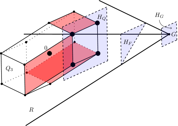
Figure 3. The hyperplanes containing the red facets of $Q_{3}$ intersect in the affine hull of face $G$ of $R$.

Case 2. See Figure 3 for an example in dimension 3. Let $x$ be an interior lattice point of $P$ closest to $F$. We may assume that $x=0$. Let $H_{F}$ be the hyperplane containing $F$. The polytope $Q_{d}$ from Definition 1.4 is contained in all alcoved $d$-polytopes which contain the origin in the interior. Any facet of an alcoved $d$-polytope is parallel to two facets of $Q_{d}$. Among the two facet-defining hyperplanes of $Q_{d}$ which are parallel to $F$, let $H_{Q}$ denote the one separating $0$ and $F$. The vertices of $Q_{d}$ on $H_{Q}$ are lattice points in $P$ which are closer to $F$ than $0$. Since $0$ is closest to $F$ among all interior lattice points of $P$, these lattice points have to be in the boundary of $P$, each of the points has to be contained in at least one facet of $P$. Consider only the facets of $P$ containing the vertices of $Q_{d}$ in $H_{Q}$ and (additionally) facet $F$. The facet-defining half-spaces of these facets define an alcoved polyhedron with $0$ in the interior. If the polyhedron $R$ obtained by removing the facet-defining half-space of $F$ from the hyperplane description of the polyhedron is unbounded in the direction of the facet normal of $F$, then by case 1 $H_{F}$ (and hence $F$) has lattice distance 1 from $0$. Assume the polyhedron $R$ is bounded in direction of the facet normal of $F$. Then there is a hyperplane $H_{G}$ parallel to $H_{F}$ which intersects $R$ in a $k$-face $G$ of $R$ and such that $H_{F}$ separates $x$ and $H_{G}$. If $H_{Q}=H_{G}$, then $H_{F}=H_{Q}$, and $H_{F}$ has distance 1 from $0$. Assume $H_{G}$ is not equal to $H_{Q}$. Then $H_{G}$ is not equal to $H_{F}$ either. We will show that $H_{G}$ has lattice distance at most $d$ from $0$, and therefore $H_{F}$ has at most lattice distance $d-1$ from $0$. $G$ is given as an intersection of $d-k$ facets of $R$. The hyperplane $H_{G}$ containing $G$ and parallel to $F$ is of the form $\{x\in\mathbb{R}^{d}\mid x_{i}-x_{j}=l\}$ for some $i,j\in\{0,\ldots,d\}$ with $i\neq j$ and $x_{0}\coloneqq 0$ and for some positive integer $l$.

We know that the difference $x_{i}-x_{j}=l$ is defined from some equations of the form $x_{s}-x_{t}=1$, for $s,t\in\{0,\ldots,d\}$ and $s\neq t$. So the difference $l$ between the two variables $x_{i}$ and $x_{j}$ can be obtained from setting the difference between some pairs of $d-1$ variables to 1. This shows that $l\in\{0,\ldots,d\}$.

We can also state this as a graph theoretical problem: Let $G$ be a simple graph on $d+1$ vertices $v_{0},\ldots,v_{d+1}$. There is an edge between vertex $v_{s}$ and vertex $v_{t}$ if and only if either $\{x\in\mathbb{R}^{d}\mid x_{s}-x_{t}=1\}$ or $\{x\in\mathbb{R}^{d}\mid x_{t}-x_{s}=1\}$ is a hyperplane of $R$ intersecting in face $G$. If $G$ would contain a cycle $(v_{s_{1}},v_{s_{2}}),(v_{s_{2}},v_{s_{3}}),\ldots,(v_{s_{r-1}},v_{s_{r}}),(v_{s_{r}},v_{s_{1}})$, then $x_{s_{1}}>x_{s_{2}}>\ldots>x_{s_{r}}>x_{s_{1}}$, a contradiction. So $G$ does not contain any cycles, it is a forest. The condition that $R$ is bounded in the direction of the facet-normal of $F$ translates to the condition that vertex $x_{i}$ and vertex $x_{j}$ are path-connected. The longest possible path-length in a forest on $d+1$ vertices is $d$. The difference $l$ is therefore at most $d$ and facet $F$ has lattice distance at most $d-1$ to $0$. ∎

We end this section with a proposition that shows that the bound from Theorem 2.7 is sharp for all dimensions $d$.

Proposition 2.8.

There is a $d$-dimensional alcoved polytope for any $d\in\mathbb{N}$ which has a facet with lattice distance $d-1$ to the interior lattice points.

Proof.

We construct an example from the following polytope: Let $P$ be the scaling of the order polytope of the chain of length $d$ by $(d+1)$:

$$P=\{x\in\mathbb{R}^{d}:x_{1} \geq 0,$$

$$x_{1} \leq x_{2},$$

$$x_{2} \leq x_{3},$$

$$\vdots$$

$$x_{d-1} \leq x_{d},$$

$$x_{d} \leq d+1\}.$$

$P$ is a reflexive alcoved simplex. The vertex description of $P$ is given by

$$P=\operatorname{conv}\{ (0,0,\ldots,0,0),(0,0,\ldots,0,d+1),\ldots,$$

$$(0,d+1,\ldots,d+1,d+1),(d+1,d+1,\ldots,d+1,d+1)\}.$$

Its unique interior lattice point is $p=(1,2,3,\ldots,d)$. The polytope $P\cap\{x\in\mathbb{R}^{d}\mid x_{1}\leq d\}$ is still an alcoved polytope with unique interior lattice point $p$. The hyperplane $\{x\in\mathbb{R}^{d}\mid x_{1}=d\}$ defining the new facet has distance $d-1$ from point $p$. ∎

For a visualization in dimension $3$, see Figure 4.

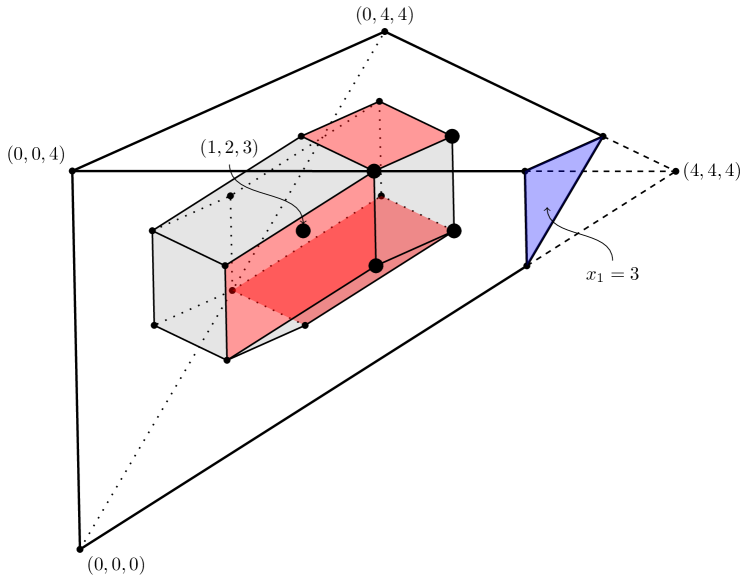
Figure 4. The blue facet has lattice distance $2$ from the interior lattice point. The red facets of $Q_{3}$ are contained in facets of the bigger polytope.

3. Computational Experiments

Here we completely list the algorithms used to calculated $h^{*}$-vectors of polytopes and test for unimodality that give the results shown in the last subsection. The code is complete so that readers can run experiments by copy-paste. All algorithms are written as SageMath code [37]. We also give some examples of alcoved polytopes and their $h^{*}$-vectors.

3.1. Convert Ehrhart polynomial to $h^{*}$-polynomial

The following program was written in collaboration with Sophia Elia. This program converts the Ehrhart polynomial of a lattice polytope to the $h^{*}$-polynomial. The Ehrhart polynomials of lattice polytopes can be calculated using LattE Integrale [4]. There is also a built-in normaliz function [12] to calculate the Ehrhart series of a polytope, but its run-time was too long for our examples.

The approach for this function is based on Eulerian polynomials (see [6, Section 2.2] The Ehrhart series can be rewritten as follows:

$$\operatorname{Ehr}_{P}(t)=\sum_{m\geq 0}L_{P}(m)t^{m}=\sum_{m\geq 0}\sum_{j\geq 0}^{d}c_{j}m^{j}t^{m},$$

where we write the Ehrhart polynomial as $L_{P}(m)=\sum_{j\geq 0}c_{j}m^{j}$. The $h^{*}$-polynomial is defined as $(1-t)^{d+1}\operatorname{Ehr}_{P}(t)$. We now exploit that the Eulerian numbers $A(d,k)$ can be defined by the generating function expression

$$\sum_{j\geq 0}j^{d}z^{j}=\frac{\sum_{k=0}^{d}A(d,k)z^{k}}{(1-z)^{d+1}}.$$

So after some calculation, we can write the $h^{*}$-polynomial as

$$h^{*}_{P}(z)=\sum_{i=0}^{d}c_{i}\left(\sum_{k=0}^{d}A(i,k)z^{k}\right)(1-z)^{d-i}.$$

We begin with a function that outputs the Eulerian numbers up to $A(n,n)$ arranged in an $(n+1)\times(n+1)$ matrix.

⬇

def eulerian_numbers(n):

A = zero_matrix(n+1,n+1)

A[0,0] = 1

for i in range(1,n+1):

A[i,0] = 0

A[i,1] = 1

for j in range(2,n+1):

for k in range(2,j+1):

if j == k:

A[j,k] = 1

else:

A[j,k] = (j-k+1)*A[j-1,k-1] +k*A[j-1,k]

return(A)

The following function makes the Eulerian polynomials based on the previous function computing the Eulerian numbers.

⬇

def eulerian_polynomial(n):

R = PolynomialRing(ZZ, ’t’)

t = R.gen()

A = eulerian_numbers(n)

return(R.sum( A[n,i]*t**i for i in range(n+1)))

Finally, here is the function that converts the Ehrhart polynomial to the $h^{*}$-polynomial. As input, it takes ehr_poly, a polynomial in t with rational coefficients. The output is the corresponding $h^{*}$-polynomial.

⬇

def ehr_to_hstar(ehr_poly):

# change the polynomial into a vector

Ring = PolynomialRing(QQbar, ’t’)

t = Ring.gen()

ehr_poly = ehr_poly.coefficients()

# get the dimension of the polytope

d = len(ehr_poly)-1

# compute the h* polynomial

factors = zero_vector(d+1)

factors = factors.change_ring(Ring)

for j in range(d+1):

factors[j] = ehr_poly[j]*(1-t)**(d-j)*eulerian_polynomial(j)

return sum(factors)

As an example, the following code verifies that the $h^{*}$-polynomial of a unimodular simplex is indeed $1$.

⬇

sage: p = polytopes.simplex(4)

sage: e = p.ehrhart_polynomial()

sage: ehr_to_hstar(e)

3.2. Random alcoved polytopes

We give an example of a function which allows us to create random alcoved polytopes. The polytopes are full-dimensional and inscribed in a cube of dimension $\dim(P)$ and with edge-length $5$ (or smaller). This is our way of making sure that the volume does not get too large for computation.

The first function organizes a list of numbers into an $\mathcal{H}$-description of an alcoved polytope. As input, it takes the dimension dim of the polytope and a vector vec of length $2\cdot\binom{\texttt{dim}}{2}+2\cdot\texttt{dim}$. The output is a matrix of size $\left(2\cdot\binom{\texttt{dim}}{2}+2\cdot\texttt{dim}\right)\times(\texttt{dim}+1)$ for the $\mathcal{H}$-description.

⬇

def alcoved_matrix(dim, vec):

c = binomial(dim,2)

M_help = Matrix (2*c,dim)

M = Matrix (2*c+2*dim,dim+1)

#

# all hyperplanes of type x_i-x_j = constant:

for i in range(c):

# all sets of 2 indices out of all indices for each choice of (x_i,x_j)

pairij = Combinations(range(dim),2).list()[i]

M_help[2*i, pairij[0] ] = 1

M_help[2*i,pairij[1] ] = -1

M_help[2*i+1, pairij[0] ] = -1

M_help[2*i+1, pairij[1] ] = 1

for i in range(2*c):

M[i, 0 ] = vec[i]

for j in range(dim): M[i,j+1] = M_help[i,j]

# all hyperplanes of type +x_i = constant

# and -x_i = constant

for i in range(2*c, 2*c+dim):

M[i, 0] = vec[i]

M[i+dim, 0] = vec[i+dim]

M[i, i+1-2*c]=-1

M[i+dim, i+1-2*c]=1

return M

The following function produces a random input vector for the previous function (satisfying the constraint that the produced alcoved polytope is contained in the appropriate cube). Its input is just the desired dimension dim of the alcoved polytope. The output is a vector of length $2\cdot\binom{\texttt{dim}}{2}+2\cdot\texttt{dim}$ that is suitable as the input vec for the previous function. The alcoved polytope generated by these two functions always contains the cube $[0,1]^{\texttt{dim}}$ and is contained in the cube $[-2,3]^{\texttt{dim}}$.

⬇

def random_vector(dim):

rand=random_matrix(ZZ, 1, 2*binomial(dim,2),

x=1,y=6).augment(random_matrix(ZZ, 1, dim, x=1,

y=4).augment(random_matrix(ZZ, 1, dim, x=0, y=3)))[0]

return rand

Alternatively, for large dimension, we might want an alcoved polytope of smaller volume. In this case, we produce a random alcoved polytope in the following way. Again, this function takes the desired dimension dim as input and outputs a vector of length $2\cdot\binom{\texttt{dim}}{2}+2\cdot\texttt{dim}$ that is suitable as the input vec for the previous function. The alcoved polytope generated by these two functions always contains the cube $[0,1]^{\texttt{dim}}$ but it is now contained in the cube $[0,3]^{\texttt{dim}}$.

⬇

def small_random_vector(dim):

rand=random_matrix(ZZ, 1, 2*binomial(dim,2), x=1,y=4).augment(random_matrix(ZZ, 1, dim, x=1,

y=3).augment(random_matrix(ZZ, 1, dim, x=0, y=2)))[0]

return rand

Finally, the following function combines the previous functions to make the polytope. As input, it takes the desired dimension dim of the alcoved polytope and it takes a vector of length $2\cdot\binom{\texttt{dim}}{2}+2\cdot\texttt{dim}$. It then makes the alcoved polytope by building its $\mathcal{H}$-description using the function shown above.

⬇

def alcoved_polytope(dim,vec):

P = Polyhedron(ieqs = alcoved_matrix(dim, vec), backend=’normaliz’)

return P

3.3. Unimodality

The programs in this section are a function that determines whether a list is unimodal and a function that tests the $h^{*}$-vectors of a given number of randomly generated alcoved polytopes of a given dimension for unimodality.
First we convert the $h^{*}$-polynomial to the $h^{*}$-vector:

⬇

# h^*-vector from h^*-polynomial

def Hvec(x): return (ehr_to_hstar(x.ehrhart_polynomial())).coefficients()

Then we determine if a list or tuple is unimodal using the following function. The input is a list or tuple ls of numbers. The output is True if the list is unimodal and False otherwise.

⬇

def unimodal(ls):

# determines index of the first decrease in the list

decr= next((i for i in range(1,len(ls)) if ls[i]-ls[i-1]<0),False)

if (decr == False) or (decr == len(ls)):

return True

else:

# determines if there is an increase after the decrease

if any(ls[i]-ls[i-1]>0 for i in range(decr+1,len(ls))):

return False

else: return True

Next we test several $h^{*}$-vectors of alcoved polytopes for unimodality. The function randomly generates alcoved polytopes specified by the input num_of_tests and dim. The first input is the number of random instances that the function generates. The second input determines the dimension. The output is the first polytope with non-unimodal $h^{*}$-vector if such a polytope is found. The output is then a vector that can be turned into a polytope with the alcoved_polytope-function described above. This function is shown here with the random_vector-function. It can, of course, also be used with the small_random_vector-function instead.

⬇

def test_for_unimodality(num_of_tests, dim):

for i in range(num_of_tests):

rv = random_vector(dim)

P = alcoved_polytope(dim,rv)

hvector = Hvec(P)

if unimodal(hvector) == False:

print(’There is an alcoved polytope with non-unimodal h-star-vector!’)

return rv

print(’All {} tested polytopes have unimodal h-star-vector.’.format(num_of_tests))

3.4. Examples

In Table 1 there are some examples of (unimodal) $h^{*}$-vectors calculated with the function Hvec coming from alcoved polytopes randomly generated with the functions described in Section 3.2.

There is one example for each dimension between 3 and 16. For dimension 16 we used the small_random_vector to generate the polytopes. For smaller dimension, we used random_vector.

Dim. $h^{*}$-vector $3$ $1,98,188,22$ $4$ $1,104,370,146,3$ $5$ $1,356,3216,3965,722,6$ $6$ $1,278,3442,7074,2977,189$ $1,522,9978,33062,$ $7$ $26037,4584,102$ $1,1962,89574,650410,$ $8$ $1210219,643554,86807,1762$ $1,$ $5624,$ $409384,$ $4544444,$ $9$ $13413250,$ $12480018,$ $3617286,$ $265589,$ $2485$ $1,$ $11361,$ $1472932,$ $26848012,$ $10$ $130799314,$ $213186186,$ $123024451,$ $23477417,$ $1154189,$ $6839$ $1,$ $14350,$ $2256181,$ $51639116,$ $327390062,$ $11$ $729687382,$ $621049446,$ $198471087,$ $20964122,$ $521849,$ $1070$

$1,$ $19944,$ $5228717,$ $186169763,$ $1812852282,$ $12$ $6346402583,$ $8965318338,$ $5257171069,$ $1223272752,$ $98031585,$ $1936661,$ $3716$ $1,$ $91329,$ $44855680,$ $2470235309,$ $35303767765,$ $180399454984,$ $13$ $380503494555,$ $350270955412,$ $139818187839,$ $22527990348,$ $1233354464,$ $15460541,$ $13816$ $1,$ $92744,$ $61035357,$ $4461610156,$ $84498080329,$ $579384773749,$ $14$ $1683186967226,$ $2226507192578,$ $1364315287619,$ $375282480730,$ $42267367262,$ $1603500992,$ $13275503,$ $6792$

$1,$ $240485,$ $278806016,$ $30713524660,$ $831462306799,$ $8037261688378,$ $33174929171015,$ $15$ $63952385251690,$ $59735193988116,$ $26931894294332,$ $5599149137353,$ $484130852634,$ $14170655809,$ $90022039,$ $36218$ $1,$ $93896,$ $91469858,$ $10614760282,$ $323897816139,$ $3658410128555,$ $18169693219004,$ $16$ $43468545132385,$ $52316695445712,$ $31944633402938,$ $9656730519861,$ $1355225501529,$ $77874204105,$ $1436104725,$ $4957986,$ $586$

Table 1. Examples of $h^{*}$-vectors

Acknowledgements. We would like to thank Christian Haase for asking the question as well as Martina Juhnke-Kubitzke and Johanna Steinmeyer for educational discussions and fruitful hints. We also profitted from the MATH+ Thematic Einstein Semester Algebraic Geometry: Varieties, Polyhedra, Computation.

References

- [1] K. Adiprasito. Combinatorial Lefschetz theorems beyond positivity, 2018. arXiv:1812.10454v4.
- [2] K. Adiprasito and G. Yashfe. The partition complex: an invitation to combinatorial commutative algebra, 2021. arXiv:2008.01044v3.
- [3] C. A. Athanasiadis. -vectors, Eulerian polynomials and stable polytopes of graphs. Electron. J. Comb., 11(2):research paper r6, 13, 2004.
- [4] V. Baldoni, N. Berline, J. A. D. Loera, B. Dutra, M. Köppe, S. Moreinis, G. Pinto, M. Vergne, and J. Wu. A User’s Guide for LattE integrale (Version 1.7.4), 2018. Available at http://www.math.ucdavis.edu/ latte/.
- [5] A. Barvinok. Lattice points and lattice polytopes. In J. Goodman, J. O’Rourke, and C. D. Tóth, editors, Handbook of Discrete and Computational Geometry, third edition, pages 185–210. Chapman & Hall / CRC Press LLC, Boca Raton, FL, 2017.
- [6] M. Beck and S. Robins. Computing the Continuous Discretely: Integer-point Enumeration in Polyhedra. Springer, 2007.
- [7] U. Betke and P. McMullen. Lattice points in lattice polytopes. Monatsh. Math., 99(4):253–265, 1985.
- [8] P. Brändén. Unimodality, log-concavity, real-rootedness and beyond. In Handbook of enumerative combinatorics, pages 437–483. Boca Raton, FL: CRC Press, 2015.
- [9] B. Braun. Unimodality problems in ehrhart theory. Recent trends in combinatorics, pages 687–711, 2016. volume 159 of IMA Vol. Math. Appl., Springer, [Cham].
- [10] F. Brenti. Log-concave and unimodal sequences in algebra, combinatorics, and geometry: an update. Jerusalem combinatorics ’93,Contemp. Math., 178.:71–89, 1994. Amer. Math. Soc., Providence, RI.
- [11] W. Bruns and J. Herzog. Cohen-Macaulay rings. Cambridge University Press, 2 edition, 2009.
- [12] W. Bruns and B. Ichim. Normaliz: Algorithms for affine monoids and rational cones. In: J. Algebra 324.5 (2010), pp. 1098–1113. Available at https://www.normaliz.uni-osnabrueck.de.
- [13] W. Bruns and T. Römer. -vectors of gorenstein polytopes. J. Combin. Theory Ser. A, 114(1):65–76, 2007.
- [14] J. De Loera, J. Rambau, and F. Santos. Triangulations: Structures for Algorithms and Applications. Algorithms and Computation in Mathematics, Vol. 25. Springer, 2010.
- [15] E. Ehrhart. Sur les polyèdres rationnels homothétiques à dimensions. C.R. Acad. Sci. Paris, 254:616–618, 1962.
- [16] C. Haase, A. Paffenholz, L. C. Piechnik, and F. Santos. Existence of unimodular triangulations – positive results. arXiv:1405.1687v3, to appear in Mem. AMS, 2017.
- [17] M. Henk and M. Tagami. Lower bounds on the coefficients of ehrhart polynomials. Eur. J. Comb., 30:70–83, 2009.
- [18] T. Hibi. Ehrhart polynomials of convex polytopes, -vectors of simplicial complexes, and nonsingular projective toric varieties. Discrete and Computational Geometry, pages 165–177, 1991. DIMACS Ser. Discrete Math. Theoret. Comput. Sci., vol. 6, Amer. Math. Soc., Providence, RI.
- [19] T. Hibi. Algebraic combinatorics on convex polytopes. Carslaw Publications, 1992.
- [20] T. Hibi and H. Ohsugi. Special simplices and gorenstein toric rings. J. Combin. Theory Ser. A, 113(4):718–725, 2006.
- [21] G. Kemper. An algorithm to calculate optimal homogeneous systems of parameters. J. Symb. Comput., 27:171–184, 1999.
- [22] M. Kubitzke and E. Nevo. The Lefschetz property for barycentric subdivisions of shellable complexes. Trans. Amer. Math. Soc., 361(11):6151–6163, Nov. 2009.
- [23] T. Lam and A. Postnikov. Alcoved polytopes I. Discrete & Computational Geometry, 38(3):453–478, 2007.
- [24] C. W. Lee. P.L.-spheres, convex polytopes, and stress. Discrete Comput. Geom., 15(4):389–421, 1996.
- [25] E. Miller and B. Sturmfels. Combinatorial Commutative Algebra. Number 227 in Graduate Texts in Math. Springer-Verlag, 2005.
- [26] M. Mustaţă and S. Payne. Ehrhart polynomials and stringy betti numbers. Math. Ann., 333(4):787–795, 2005.
- [27] S. Payne. Ehrhart series and lattice triangulations. Discrete Comput. Geom., 40(3):365–376, 2008.
- [28] G. A. Reisner. Cohen-Macaulay quotients of polynomial rings. Adv. Math., 21:30–49, 1976.
- [29] J. Schepers and L. V. Langenhoven. Unimodality questions for integrally closed lattice polytopes. Ann. Comb., 17:571–589, 2013.
- [30] R. Stanley. Combinatorics and Commutative Algebra. Progress in Mathematics, Vol. 41. Birkhäuser Basel, 1996. Second Edition.
- [31] R. P. Stanley. The Upper Bound Conjecture and Cohen-Macaulay rings. Studies in Appl. Math., 54:135–142, 1975.
- [32] R. P. Stanley. Decompositions of rational convex polytopes. Ann. Discrete Math., 6:333–342, 1980.
- [33] R. P. Stanley. The number of faces of simplicial convex polytopes. Advances in Math., 35:236–238, 1980.
- [34] R. P. Stanley. Log-concave and unimodal sequences in algebra, combinatorics, and geometry. Annals of the New York Academy of Sciences, 576(1):500–535, 1989.
- [35] R. P. Stanley. A monotonicity property of h-vectors and h*-vectors. European Journal of Combinatorics, 14(3):251–258, 1993.
- [36] J. Steinmeyer. Personal communication.
- [37] The Sage Developers. SageMath, the Sage Mathematics Software System (Version 9.0), 2020. Available at https://www.sagemath.org.